Finding analytical approximations for discrete, stochastic, individual-based models of ecology

We consider a model where individuals live on a $D\times D$ lattice with cyclic boundary conditions. There a thus a total of $n=D^{2}$ resource sites. We divide the life cycle of the individuals into a competition phase, a reproduction phase and a dispersal phase. Let $X_{ij}^{t}$ be a random variable denoting the number of individuals at site $(i,j)$ at time $t$. At the competition phase there may be more than one individual at a particular site. In order to capture competition for resources we define a survival function $\phi:\mathbb{N}\rightarrow\{0,1\}$ that acts on $X_{ij}^{t}$ giving a new site population $\phi(X_{ij}^{t})$. The survival function maps the number of individuals at a given site to 0 if the site is over exploited or 1 if there is a survivor. This captures over-crowding: if there are too many individuals at a resource site, they cannot all reproduce.

After competition the next phase is reproduction. The surviving individual at a site (if there is one) produces $R_{ij}^{t}$ offspring, where $R_{ij}^{t}$ is a random variable with expectation $\Ex[R_{ij}^{t}]=r$ for all $i$, $j$ and $t$. We consider discrete generations, so after the reproduction phase the parents die, resulting in $R_{ij}^{t}\cdot\phi(X_{ij}^{t})$ individuals at each site $(i,j)$. These offspring then disperse to a random site in a $(2s+1)\times(2s+1)$ Moore neighbourhood, with uniform probability, resulting in a new site count $X_{ij}^{t+1}$. The Moore neighbourhood of site $(i,j)$ with range $s$, $N(i,j,s)$, is given by the set of sites $(i^{\prime},j^{\prime})$ for which $|i-i^{\prime}|\leq s$ and $|j-j^{\prime}|\leq s$. Since the lattice has cyclic boundary conditions, individuals leaving the lattice in one end, end up on the opposite side, i.e. two sites $(i,j)$ and $(i^{\prime},j^{\prime})$ are identical if $i\ (\mathrm{mod}\ D)=i^{\prime}\ (\mathrm{mod}\ D)$ and $j\ (\mathrm{mod}\ D)=j^{\prime}\ (\mathrm{mod}\ D)$. The life cycle is complete and the process starts over again.

There are several ways to define the survival function and Brännström and Sumpter 2005b examine the population dynamics for different survival functions for the non-spatial case. In our simulations of this individual-based model, however, we will define the survival function as

$$\phi(k)=\begin{cases}1&\mbox{if }k=1\\ 0,&\text{otherwise},\end{cases}$$

(1)

which gives a classic scramble competition model, as first described by Nicholson 1954. In our simulations in the main article, we also assume $R_{ij}^{t}$ to be equal to a constant $r$ for all $i$, $j$ and $t$, and not random variable. In Supplementary material S3 we simulate the model for $R_{ij}^{t}\sim\operatorname{Bin}(r/q,q)$, for different values of $q$. Figure 1 illustrates the individual-based model with scramble competition for $r=4$ and $s=2$. Individuals that are alone in a site survive, whereas in sites with more than one individual, all individuals die. The surviving individuals then produce $r=4$ offspring each, that disperse to a randomly chosen site with uniform probability in a $(2s+1)\times(2s+1)$ Moore neighbourhood.

The model has a rich set of dynamics depending on the parameter values $r$ and $s$. Figure 2 shows how the spatial distribution of individuals on a $101\times 101$ lattice evolves over time for four time steps for different values of $s$, when $r=20$. When $s=1$, there is no clear spatial clustering, and between generations the population is relatively stable. As $s$ increases to 2 and 3 (Figure 2 (b)-(c)), we can distinguish spatial clusters. While the overall population size is still reasonably stable over time, there are local fluctuations. Patches of a size roughly $(2s+1)\times(2s+1)$, i.e. the same size as the dispersal range emerge creating a checkerboard effect. In Figure 2 (d) and (e), where $s=5$ and $s=10$ respectively, the global population is the global population is alternatingly large and small and fluctuates in the four consecutive snapshots. The last figure, Figure 2 (f), shows time evolution of the population for $s=50$. Dispersal is now global, i.e. individuals disperse uniformly to any site on the lattice, since $s=(D-1)/2=50$ for $D=101$. The figure displays chaotic oscillations between generations and there is no spatial clustering.

Further simulations are summarised in bifurcation plots shown in Figure 3. Here we varied $r$, simulated the model for 5000 time steps, and the plot shows the outcome for the last 500 time steps. In Figure 3 (a), we see how very local dispersal ($s=1$) typically gives rise to a stable population. This population reaches a maximum at around $r\approx 15$, and it dies out at $r=23$. Figure 3 (b)-(c) shows a stable population for $s=2$ and $s=3$. Increasing $s$ to 5, there is a period doubling when $r=9$, and for $s=10$, the period doubling bifurcation occurs already at $r=8$, which we see in Figure 3 (d) and (e). When dispersal is global the population is stable for $r<e^{2}(\approx 7.39)$, and undergoes a period doubling bifurcation after that, leading to an oscillating population size between generations when $8<r<14$. When $r>15$ the population oscillates chaotically. In summary, for all values of $s$, the population is stable for small reproductive rates, but for higher values of $r$, the population goes from stable to oscillating to chaotic by increasing $s$.

In Supplementary material S3 we look at what happens to the dynamics if the reproductive rate is not constant, but instead the reproductive rate at each site and time step, $R_{ij}^{t}$, are i.i.d with $R_{ij}^{t}\sim\operatorname{Bin}(r/q,q)$, by producing bifurcation plots for different values of $s$ and $q$. We see that the overall behaviour is not affected by different values of $q$.

Increasing the lattice size to $201\times 201$ and the reproductive rate to $r=30$, the individual-based model produces interesting patterns, which is seen in Figure 4. When $s=10$, we see oscillating ring patterns, resembling reaction-diffusion patterns. As we increase $s$ to 20, the population dynamics instead behave as travelling waves. When $s=45$ there is a band formation jumping between the two halves of the lattice in each consecutive snapshot. In Figure 4 (c) the band formation is vertical, but the band formation can also be horizontal.

In the bifurcation diagram in Figure 5 (a) ,we fixed $r$ to 30 and varied $s$, simulated the model for 5000 time steps, and the plot shows the outcome for the last 500 time steps. From this bifurcation diagram, we can conclude that the band formation seen in Figure 4 (c) gives rise to stable population dynamics. For $s=10$, the population dynamics seem stable and for $s=20$ the population is fluctuating. In the bifurcation diagram in Figure 5 (b), we instead fixed $s$ to 45 and varied $r$, simulated the model for 5000 time steps, and the plot shows the outcome for the last 500 time steps. We see that the population is stable for $r<8$, and exhibits a period doubling bifurcations after that. At $r=22$, the population becomes stable again. We can thus see that long-range, but not global, dispersal has a stabilizing effect on the population dynamics for high reproductive rates.

In essence, the snapshots of the model together with the bifurcation plots, show that our model displays behaviour which are inherently discrete in time: the population density display chaotic behaviour for some values of $r$ and $s$, and there are large-scale discrete oscillations in the spatial distribution of the population, rather than waves that move smoothly.

The snapshots of the individual-based model, together with the bifurcation diagrams, demonstrate that spatial structure strongly influence the population dynamics. In Section 3 we will make different assumptions of the spatial distribution of the individual-based model, in order to find analytical approximations of the model. Thus, understanding the spatial structure and scales of the individual-based model is valuable for the approximations done in 3. In the supplementary material S1, we use Moran’s $I$ (which measures spatial correlation) to show that spatial clustering changes with dispersal distance. This, in itself, does not give us any information of the scales of the spatial clusters. A better measure for detecting spatial pattern scales is the four-term local quadrat variance measure, referred to as 4TLQV. The idea behind 4TLQV is to look at a block of size $b\times b$ and then compare this block to three adjacent blocks. This is done by summing all the individuals in the first block, multiply by $-3$ and then sum all individuals of the other three blocks. Since any of the four blocks can be used for comparison, there are four possible ways to do this calculation, and the 4TLQV is calculated by taking the average of the squared values of these four possibilities (see the Figure S3 for an illustration of this). The peaks in 4TLQV as a function of $b$ can be interpreted as the spatial scale of the pattern. We used the PySSaGE package for Python, to calculate the 4TQLV for 100 consecutive snapshots of 10 realisations of the individual-based model for various values $s$ (i.e. 1000 snapshots for each parameter set) (Rosenberg 2021).

In Figure 6 we see the average 4TQLV of 100 consecutive snapshots from 10 realisations (1000 snapshots in total) for different values of $s$ when $r=20$ as a function of the block size, $b$. We note that for $s=1$ and $s=2$, the peak in variance is already at $b=1$, suggesting that there is no clear spatial structure. For $s=3$, there is a peak around $b=9$. As $s$ increases, the value of the 4TLQV peak also increases. However, when $s=50$ the peak is now at $b=1$, suggesting there is no clear spatial structure.

In Figure 7, the average 4TLQV variance is plotted for different values of $s$ when $r=30$ and the lattice size is $201\times 201$. We see that when $s=10$, there is a peak around $b=30$. For $s=20$, there are there is a peak around 60, and for $s=45$, there is a peak at $b=90$. What should also be noted, but is not shown here, is that for all parameter sets with clear spatial patterns, the variance of the 4TLQV increases as $b$ increases, meaning that the spatial patterns sizes varies between time step. From these plots, we can conclude that if there is a spatial pattern, the size of the pattern is always larger than $2s+1$. This is not surprising, since the individuals disperse into a $(2s+1)\times(2s+1)$ blocks and thus compete with other individuals within that range, the spatial patterns should be at least of that size.

We start with the model described in Section 2 with scramble competition described by equation (1). Let $x_{t}$ be the density of the population at time $t$, where $t=0,1,2,...$ is the time after the competition phase, i.e. after the survival function $\phi(X_{ij}^{t})$ has been applied to every resource site. The expected population density at time $t+1$ given the population density $x_{t}$ at time $t$ can be written as:

$$x_{t+1}=\Ex(X_{t+1}|X_{t}=x_{t})=\frac{1}{D^{2}}\sum_{k=1}^{\infty}\sum_{i=1}^{D}\sum_{j=1}^{D}P(X_{ij}^{t}=k|X_{t}=x_{t})\cdot\phi(k).$$

(2)

Here $\phi(k)$ is the survival function and $P(X_{ij}^{t}=k|X_{t}=x_{t})$ is the probability to find $k$ individuals in a site $(i,j)$ at time $t$, given that the population density is $x_{t}$. The question of approximating the population dynamics becomes a question of finding a good approximation $p_{k}$ of $P(X_{ij}^{t}=k)$, which utilises as much information as possible about the correlations between neighbouring sites. Thus $p_{k}$ is an approximation of $P(X_{ij}^{t}=k)$, which is not dependent on a specific site $(i,j)$. From this, we can reduce equation (2) to

$$x_{t+1}=\frac{1}{D^{2}}\sum_{k=1}^{\infty}\sum_{i=1}^{D}\sum_{j=1}^{D}p_{k}\cdot\phi(k)=\sum_{k=1}^{\infty}p_{k}\cdot\phi(k),$$

(3)

i.e. $p_{k}$ is site independent.

One possible way to approximate $p_{k}$, is to assume that the offspring disperse independently to any site on lattice with uniform probability. When the lattice is infinitely large, $X_{ij}^{t}$ is Poisson distributed with mean $rx_{t}$ for all $i$ and $j$, in which case

$$p_{k}=P(X_{ij}^{t}=k)=\frac{e^{-rx_{t}}(rx_{t})^{k}}{k!},$$

(4)

giving the following population dynamics

$$x_{t+1}=\sum_{k=1}^{\infty}\frac{e^{-rx_{t}}(rx_{t})^{k}}{k!}\cdot\phi(k).$$

(5)

In this case, the entire population dynamics for the scramble model is

$$x_{t+1}=rx_{t}e^{-rx_{t}}.$$

(6)

This equation, sometimes called the mean field equation (Morozov and Poggiale 2012), we refer to as the global approximation equation of the individual-based model. This is the same equation as derived by Sumpter and Broomhead 2001 and Brännström and Sumpter 2005a but with a change of variable $x_{t}^{\prime}=rx_{t}$ to reflect the fact that we measure the population after reproduction. This global approximation works well for individual-based models with large dispersal, i.e. when $s$ is close to $(D-1)/2$.

From the simulations of the individual-based model, we saw that even though the scale of the spatial pattern is the same for very local dispersal ($s=1$ and $s=2$) and global dispersal, the population dynamics is vastly different: when dispersal is global, the population dynamics is chaotic, whereas the population dynamics is always stable for local dispersal. This suggests, that for local dispersal, ($s<<D$), we need to take local correlations into account. To do this, we adopt an approach that looks at correlations which arise between dispersal and competition. Consider a particular lattice site, which we call the focal site. In order to better account for local correlations we look in the $(2s+1)\times(2s+1)$ Moore neighbourhood around the focal site. Let $F$ be the total number of parents in the $(2s+1)\times(2s+1)$ Moore neighbourhood of the focal site (see Figure 8).

For this approximation we assume – as we also did in our approximation of full independence between the sites – that the population is uniformly distributed at this stage with population density $x_{t}$. The spatial statistics in Section 2.3 together with the supplementary material S1, showed that this assumption is justified not just for global dispersal, but also for very local dispersal (i.e. when $s$ is small). Now, if $s<<D$, we can assume that each site in the neighbourhood of the focal site has an independent probability $p=x_{t}$ containing an individual, meaning that $F\sim\operatorname{Bin}((2s+1)^{2},x_{t})$. In this new approximation, our aim is to calculate the number of offspring of all of the parents in the neighbourhood of the focal site that disperse to the focal site. We denote this as a random variable $Y$. The probability that a particular offspring of a particular parent within the $(2s+1)\times(2s+1)$ Moore neighbourhood ends up in the focal site is $1/(2s+1)^{2}$. We can thus denote the event that this offspring $j$ lands on the focal site as a Bernoulli random variable, $O_{j}$ with parameter $1/(2s+1)^{2}$. The dispersal of individuals is independent and thus $Y$ is defined by the sum

$$Y=\sum_{j=1}^{F\cdot r}O_{j}$$

(7)

or, equivalently, $Y\sim\operatorname{Bin}(F\cdot r,\frac{1}{(2s+1)^{2}})$.

Using the law of total probability we utilise equation (7) to write

$$p_{k}=P(Y=k)=\sum_{i=1}^{(2s+1)^{2}}P(Y=k|F=i)P(F=i).$$

(8)

The two terms in this convolution are, respectively,

$$P(Y=k|F=i)=\binom{ir}{k}\frac{1}{(2s+1)^{2k}}(1-\frac{1}{(2s+1)^{2}})^{ir-k},$$

(9)

and

$$P(F=i)=\binom{(2s+1)^{2}}{i}x_{t}^{i}(1-x_{t})^{(2s+1)^{2}-i}.$$

(10)

This gives the following explicit expression for $p_{k}$

$$p_{k}=\sum_{i=1}^{(2s+1)^{2}}\binom{(2s+1)^{2}}{i}x_{t}^{i}(1-x_{t})^{(2s+1)^{2}-i}\binom{ir}{k}\frac{1}{(2s+1)^{2k}}\left(1-\frac{1}{(2s+1)^{2}}\right)^{ir-k}.$$

(11)

With the approximation that all sites on the lattice experience the same dynamics as the focal site, the population dynamics are then given by

$$x_{t+1}=\sum_{k=1}^{\infty}p_{k}\cdot\phi(k).$$

(12)

For scramble competition, where $\phi(k)$ is defined as equation (1), the expression becomes

$\displaystyle x_{t+1}$

$\displaystyle=\sum_{i=1}^{(2s+1)^{2}}\binom{(2s+1)^{2}}{i}x_{t}^{i}(1-x_{t})^{(2s+1)^{2}-i}ir\frac{1}{(2s+1)^{2}}(1-\frac{1}{(2s+1)^{2}})^{ir-1}.$

(13)

By identifying the last factor as a derivative, the expression can be simplified to

$\displaystyle x_{t+1}$

$\displaystyle=rx_{t}\left(1-\frac{1}{(2s+1)^{2}}\right)^{r-1}\left(x_{t}\left(1-\frac{1}{(2s+1)^{2}}\right)^{r}-x_{t}+1\right)^{(2s+1)^{2}-1}=f(x_{t}).$

(14)

We now have a better approximation of the individual-based model that, unlike the global approximation equation (equation (6)), takes in the spatial properties of the individual-based model, and has the dispersal distance, $s$, as a parameter. (See Supplementary material S4 for a detailed derivation.)

Now, if $R_{ij}^{t}$ is not constant, but $R_{ij}^{t}$ are i.i.d. random variables with $R_{ij}^{t}\sim\operatorname{Bin}(r/q,q)$, the number of offspring the parents will produce will be given by

$$S_{F}=\sum_{i}^{F}R_{i}$$

(15)

where $R_{i}\sim\operatorname{Bin}(r/q,q)$. Thus,

$$Y=\sum_{j=1}^{S_{F}}O_{j}=\sum_{j=1}^{\sum_{i}^{F}R_{i}}O_{j}.$$

(16)

Using probability generating functions (see Supplementary material S4), we can find a closed form of $p_{1}=P(Y=1)$, which will be given by

$$p_{1}=rx_{t}\left(\left(1-\frac{1}{(2s+1)^{2}}\right)q-q+1\right)^{r/q-1}\\ \left(x_{t}\left(\left(1-\frac{1}{(2s+1)^{2}}\right)q-q+1\right)^{r/q}-x_{t}+1\right)^{(2s+1)^{2}-1}.$$

(17)

Thus, when the reproductive rate, $R_{ij}^{t}$, is random with $R_{ij}^{t}\sim\operatorname{Bin}(r/q,q)$, the population dynamics is given by

$$x_{t+1}=rx_{t}\left(\left(1-\frac{1}{(2s+1)^{2}}\right)q-q+1\right)^{r/q-1}\\ \left(x_{t}\left(\left(1-\frac{1}{(2s+1)^{2}}\right)q-q+1\right)^{r/q}-x_{t}+1\right)^{(2s+1)^{2}-1}.$$

(18)

In the rest of the paper, we will focus on the analysis of model with deterministic $r$, but in Supplementary material S4, derive and analyse the local correlation approximation with random $R$.

The bifurcation diagram in Figure 5 shows that for long-range dispersal, i.e., $s\approx D/2$, the population density stabilizes. The four consecutive snapshots of the individual-based model for $s=45$ in Figure 4 (c) suggests that this happens when the population propagates as a band over the lattice, i.e., when the spatial pattern scale is around $D/2$, as seen in Figure 7 (c). Even though there is a clear global spatial structure in terms of the band formation, calculating the Moran’s $I$ within each band, suggest that the population is close to well mixed locally.

To capture this observation, we propose a long-range dispersal approximation, which divides the lattice into two patches, $P_{1}$ and $P_{2}$, with population size $x_{1}$ and $x_{2}$ respectively, with dispersal probability $\delta$ between the patches, as seen in Figure 9. In this approximation, the population is assumed large and well mixed within each patch, allowing us to describe the population as a coupled version of the global approximation (Eq. (6)), i.e.

$$\begin{split}x_{1,t}=(1-\delta)re^{-rx_{1,t}}+\delta re^{-rx_{2,t}}\\ x_{2,t}=(1-\delta)re^{-rx_{2,t}}+\delta re^{-rx_{1,t}}.\end{split}$$

(19)

We now want to determine reasonable values of the dispersal probability $\delta$ as a function of the dispersal distance $s$, by reasoning from the individual-based model. For simplicity, we assume that an individual in $P_{1}$ enters $P_{2}$ only when it crosses the border in the middle. When crossing the other borders, it re-enters $P_{1}$. Since $P_{1}$ and $P_{2}$ are identical except for being laterally reversed, it suffices to determine the dispersal probability from $P_{1}$ to $P_{2}$ to find $\delta$. To do this, we start by indexing the sites by $(i,j)$, as in Figure 9. In $P_{1}$ we have $1\leq i\leq D/2$ and $1\leq j\leq D$. The dispersal probability between $P_{1}$ and $P_{2}$ will be given by the probability that an individual $k$ is situated at site $(i,j)$ times the probability that it disperses to patch $P_{2}$, given that it is at site $(i,j)$, summed over all sites in $P_{1}$:

$$\begin{split}\delta&=\sum\limits_{(i,j)\in P_{1}}P(k\text{ at site }(i,j)|\text{ }k\text{ in }P_{1})\cdot P(k\text{ disperse to }P_{2}|\text{ }k\text{ at site }(i,j)).\end{split}$$

(20)

Assuming that within each patch the population is well mixed, meaning that individuals are uniformly distributed over all sites, we have that $P(k\text{ at site }(i,j)|\text{ }k\text{ in }P_{1})$ is given by $\frac{1}{D^{2}/2}$.

To determine $P(k\text{ disperse to }P_{2}|k\text{ at site }(i,j))$, we want to find the number of sites in $P_{1}$ where $P_{2}$ is reachable by dispersal. This obviously depends on $s$. We have that

$$P(k\text{ disperse to }P_{2}|\text{ at site }(i,j))=\frac{(s+1)-i}{2s+1},$$

when $i<s$, and $0$ when $i>s$.

Thus, we have

$$\begin{split}\delta&=\sum\limits_{(i,j)\in P_{1}}P(k\text{ at site }(i,j)|k\text{ in }P_{1})\cdot P(k\text{ disperse to }P_{2}|k\text{ at site }(i,j))\\ &=\sum\limits_{j=1}^{D}\sum\limits_{i=1}^{D/2}\frac{1}{D^{2}/2}P(k\text{ disperse to }P_{2}|k\text{ at site }(i,j))\\ &=D\sum\limits_{i=1}^{D/4}\frac{1}{D^{2}/2}P(k\text{ disperse to }P_{2}|k\text{ at site }(i,j))=2D\sum\limits_{i=1}^{D/4}\frac{(s+1)-i}{2s+1}\\ &=\frac{s(s+1)}{D(2s+1)}.\end{split}$$

(21)

We now have three different approximations that describe the population dynamics for the individual-based model. For the rest of the paper we will analyse equation (14), (19) and (6) and compare it with the individual-based model described in Section 2.

As for the individual-based model in Figure 3, we produced bifurcation plots for the local correlation approximation by iterating equation (14) for different values of $r$, which can be seen in Figure 10. When dispersal is very local ($s=1$), our approximation displays quantitatively the same behaviour as the individual-based model: the population is stable and at most around 2 (when $r\approx 15$). The only difference between the individual-based model and the local correlation approximation is that the population goes extinct already at $r=23$ for the individual-based model, whereas it goes extinct for $r=30$ for the approximation. In Figure 10 (b), we see that there is a period doubling bifurcation when $r=10$, for $s=2$, in contrary to the individual-based model, where the population is stable at least until $r=30$ for $s=2$. Increasing $s$ to 3 (Figure 10 (c)), the approximation model undergoes a period-doubling route to chaos: the model exhibits period doubling first at $r=8$ and then at $r=16$, and becomes chaotic at $r=26$. Increasing $s$ further, the period doubling takes place earlier and earlier: in Figure 10 (d) we see that for $s=5$, the first period doubling appears at $r=8$ and the second at $r=13$. For $s=10$, the dynamics of the approximation is more or less the same as for $s=50$. Quantitatively, the population density is higher for the local correlation approximation, than for the individual-based model, when $s>2$. In summary, the local approximation seem to approach the global approximation quicker than the individual-based model approaches the well-mixed case. In Supplementary material S4 we show bifurcation plots for the local correlation approximation for stochastic reproductive rates, i.e. equation (S11). We see in the plots that over all qualitative behaviour is not affected by the value of $q$, just as for the bifurcation plots of the individual-based model with stochastic reproductive rate.

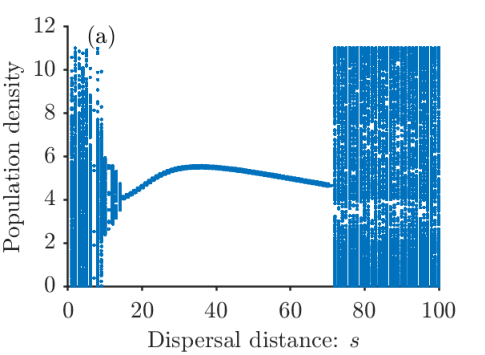
For the long range dispersal approximation, we produced bifurcation plots with both $s$ and $r$ as the bifurcation parameter. In Figure 11 (a), we see that for $s$ between 40 and 50, the approximation has both quantitatively and qualitatively the same behaviour as the individual-based model: the population is stable and has a size around 4. However, in contrast to the individual-based model, the long-range dispersal approximation exhibits a stable population already at $s=15$ and up until $s=70$.

One important property of the individual-based model, that is not captured in the global approximation equation, is that the population goes extinct for some values of $r$, both when $s$ is very local ($s=1$) and when $s$ is global,as seen in Figure 3 (a) and (f). We want to find for which values of $r$ this happens for the local correlation approximation. To do so, we first observe that $x_{*}=0$ is always a steady state for equation (14). We then check the stability for the steady state $x_{*}=0$. Differentiating $f(x_{*})$ we obtain:

$$f^{\prime}(x_{*})=r\left(\frac{(2s+1)^{2}-1}{(2s+1)^{2}}\right)^{r-1}\left(x_{*}\left(\left(\frac{(2s+1)^{2}-1}{(2s+1)^{2}}\right)^{r}-1\right)+1\right)^{(2s+1)^{2}-2}\left((2s+1)^{2}x_{*}\left(\left(\frac{(2s+1)^{2}-1}{(2s+1)^{2}}\right)^{r}-1\right)+1\right)$$

(22)

When $x_{*}=0$, we have

$$f^{\prime}(0)=r\left(\frac{(2s+1)^{2}-1}{(2s+1)^{2}}\right)^{r-1}=r\left(1-\frac{1}{(2s+1)^{2}}\right)^{r-1}.$$

(23)

The stability condition $|f^{\prime}(x_{*})|<1$ for $x_{*}=0$ yields

$$\left|r\left(1-\frac{1}{(2s+1)^{2}}\right)^{r-1}\right|<1,$$

(24)

which, for $s=1$, is true for $1<r<30$. Thus, for our local correlation approximation, the population goes extinct when $r>30$, which is seen in Figure 10 (a). This is a slightly larger value than what is seen in bifurcation diagram of the individual-based model (Figure 3 (a)), where, after $t=5000$ time steps, extinction is observed already for $r=23$. When $s$ increases, the extinction value for $r$ in the local correlation approximation increases as well. In Figure 12 (a), we see how the value of $s$ affects $f^{\prime}(x_{*})$ when $x_{*}=0$. For $s=2$ e.g., $r$ needs to be larger than $117$ for the population to go extinct. For global dispersal, we have that

$$\lim_{s\to\infty}f^{\prime}(0)=\lim_{s\to\infty}r\left(1-\frac{1}{(2s+1)^{2}}\right)^{r-1}=r,$$

(25)

and thus the inequality (24) is only fulfilled for $r<1$. This means that the local correlation approximation never result in extinction for global dispersal. In Figure 12 below, we see a graphical illustration of this: when $s=1$, $f^{\prime}(x_{*})$ crosses the line $y=1$ when $r=30$. As $s$ increases, the slope of $f^{\prime}(x_{*})$ increases. For the global approximation equation, $f^{\prime}(x_{*})=r$, and will thus never cross the line $y=1$. In Figure 12 (b) we see $f(x_{t})$ as a function of $x_{t}$ when $r=20$ and for different values of $s$. In this cobweb diagram, we see that the population dynamics becomes unstable as $s$ increases.

Now for our local correlation approximation with $R_{ij}^{t}\sim\operatorname{Bin}(r/q,q)$, given by equation (S11), $x_{*}=0$ will also be a steady state, and $f^{\prime}(x_{*})|_{x^{*}=0}$ will be given by

$$f^{\prime}(x_{*})|_{x^{*}=0}=r\left(1-\frac{q}{(2s+1)^{2}}\right)^{r/p-1}.$$

(26)

The stability of $x_{*}=0$ of the local correlation approximation for stochastic reproductive rate will thus be affected by the value of $q$, and for smaller values, the population will become extinct for higher $r$ values.

The individual-based model clearly displays population extinction for some values of $r$ when dispersal is global, as seen in the bifurcation diagram in Figure 3(f). However, this extinction is not due to the stability of the stationary point $x_{*}=0$, but due to the stochasticity of the individual-based model: when $r$ is sufficiently large there is always a probability that all sites get overcrowded in one generation and the population goes extinct. We now want to find for which values of $r$ this happens. To find an expression for this, we make use of the different life-cycle stages within one time step: the population before competition, the population after competition but before reproduction, and the population after reproduction. Consider the individual-based model with $n=D\times D$ resource sites. For the population to survive after competition, at least one resource site must contain exactly one individual (in case of scramble competition). Let $x_{t}$ be the number of individuals before competition and reproduction at generation $t$, and $x_{t^{\prime}}$ be the number of individuals after reproduction in the same time step. When dispersal is global, the probability that a particular resource site contains exactly one individual, $P(X=1)$, will be a function of $x_{t}$, $p_{1}(x_{t})$, since $X$ is Poisson distributed with mean $x_{t}/n$. We can thus write

$$p_{1}(x_{t})=\frac{x_{t}}{n}e^{-\frac{x_{t}}{n}}.$$

(27)

$p_{1}(x_{t})$ will be maximized at $x_{t}=n$:

$$p_{1}(n)=\frac{n}{n}e^{-\frac{n}{n}}=e^{-1}=p_{1}^{*}.$$

(28)

Thus $p_{1}^{*}>p_{1}(x_{t})$ $\forall x_{t}$. When this is maximized, there will be $e^{-1}\cdot n$ individuals that survived after competition, meaning that, if the reproductive rate is constant, there will be

$$x_{t^{\prime}}=nre^{-1}$$

(29)

individuals after reproduction. Thus, the probability for a particular resource site containing exactly one individual after reproduction

$$p_{1}(x_{t^{\prime}})=\frac{nre^{-1}}{n}e^{-\frac{nre^{-1}}{n}}=re^{-1}e^{-re^{-1}}.$$

(30)

Then the probability that none of the resource sites has exactly one individual is given by

$$p_{\text{extinct}}^{*}=(1-p_{1}(x_{t^{\prime}}))^{n}=(1-re^{-1}e^{-re^{-1}})^{n}.$$

(31)

Since $p_{1}^{*}>p_{1}(x_{t})$ $\forall x_{t}$, $p_{\text{extinct}}^{*}<p_{\text{extinct}}(x_{t^{\prime}})$ $\forall x_{t}$. Thus, this is the minimum probability of going extinct for each generation. In Figure 13 we see how this probability is affected for different values of $D$ and $r$, and how this is connected to the actual simulations of the individual-based model (the black line and error bar). Recall that $p_{\text{extinct}}$ is the minimum probability of going extinct at each time step, and thus when simulating over many generations (below for 5000 generations), the population will go extinct when $p_{\text{extinct}}$ is quite low ($\approx 0.1$).

When deriving the local correlation approximation, we made the assumption that $s<<D$. However Figures 10 and 12 (a) suggest that as $s$ increases the equation (14) comes increasingly close to the global approximation (equation (6)). Indeed, when $s=50$ in Figure 12 (b), the curve defined by equation (14) is indistinguishable from the global approximation equation. These numerical results suggest that when $s$ is large, the local correlation approximation reproduces the dynamics of the global approximation, even though the $s<<D$ assumption that was made for the approximation is not fulfilled. To rigorously determine whether this result holds, we need to check if our population dynamics model in equation (14) approaches the original global approximation as $s\to\infty$. This is equivalent to showing that the limit $\lim_{s\to\infty}Y\rightarrow\text{Po}(rx_{t})$, in distribution. Here $Y$ is the number of offspring of all of the parents in the $(2s+1)\times(2s+1)$ Moore neighbourhood of a focal site that disperse to the focal site. Thus, $\lim_{s\ to\infty}Y\rightarrow\text{Po}(rx_{t})$, means that when dispersal is global the number of offspring from the whole lattice that end up in a particular site, is Poisson distributed with mean $rx_{t}$. To show this limit, we can make use of the following theorem:

The total variation distance is a measure of the closeness of two probability distributions. Intuitively, the total variation distance between two probability distribution is the largest possible difference that the two probability distributions can assign to the same event. Thus, a total variation distance equal to zero, indicates that the probability distributions are the same.

References

- Anazawa (2009) M. Anazawa. Bottom-up derivation of discrete-time population models with the allee effect. Theoretical population biology, 75(1):56–67, 2009.
- Anazawa (2014) M. Anazawa. Individual-based competition between species with spatial correlation and aggregation. Bulletin of mathematical biology, 76(8):1866–1891, 2014.
- Berec (2002) L. Berec. Techniques of spatially explicit individual-based models: construction, simulation, and mean-field analysis. Ecological modelling, 150(1-2):55–81, 2002.
- Boerlijst et al. (1993) M. C. Boerlijst, M. E. Lamers, and P. Hogeweg. Evolutionary consequences of spiral waves in a host—parasitoid system. Proceedings of the Royal Society of London. Series B: Biological Sciences, 253(1336):15–18, 1993.
- Bolker and Pacala (1997) B. Bolker and S. W. Pacala. Using moment equations to understand stochastically driven spatial pattern formation in ecological systems. Theoretical population biology, 52(3):179–197, 1997.
- Bordj and El Saadi (2022) N. Bordj and N. El Saadi. Moment approximation of individual-based models. application to the study of the spatial dynamics of phytoplankton populations. Applied Mathematics and Computation, 412:126594, 2022.
- Brännström and Sumpter (2005a) Å. Brännström and D. J. Sumpter. Coupled map lattice approximations for spatially explicit individual-based models of ecology. Bulletin of mathematical biology, 67(4):663–682, 2005a.
- Brännström and Sumpter (2005b) Å. Brännström and D. J. Sumpter. The role of competition and clustering in population dynamics. Proceedings of the Royal Society of London B: Biological Sciences, 272(1576):2065–2072, 2005b.
- Brown and Brown (1996) C. R. Brown and M. B. Brown. Coloniality in the cliff swallow: the effect of group size on social behavior. University of Chicago Press, 1996.
- Costa and Costa (2006) J. T. Costa and J. T. Costa. The other insect societies. Harvard University Press, 2006.
- DeAngelis (2018) D. L. DeAngelis. Individual-based models and approaches in ecology: populations, communities and ecosystems. CRC Press, 2018.
- DeAngelis and Yurek (2017) D. L. DeAngelis and S. Yurek. Spatially explicit modeling in ecology: a review. Ecosystems, 20(2):284–300, 2017.
- Dieckmann et al. (2000) U. Dieckmann, R. Law, and J. A. Metz. The geometry of ecological interactions: simplifying spatial complexity. Cambridge University Press, 2000.
- Durrett (1999) R. Durrett. Stochastic spatial models. SIAM review, 41(4):677–718, 1999.
- Durrett and Levin (1994) R. Durrett and S. Levin. The importance of being discrete (and spatial). Theoretical population biology, 46(3):363–394, 1994.
- Ermentrout and Edelstein-Keshet (1993) G. B. Ermentrout and L. Edelstein-Keshet. Cellular automata approaches to biological modeling. Journal of theoretical Biology, 160(1):97–133, 1993.
- Gyllenberg et al. (1993) M. Gyllenberg, G. Söderbacka, and S. Ericsson. Does migration stabilize local population dynamics? analysis of a discrete metapopulation model. Mathematical Biosciences, 118(1):25–49, 1993.
- Hall-Stoodley et al. (2004) L. Hall-Stoodley, J. W. Costerton, and P. Stoodley. Bacterial biofilms: from the natural environment to infectious diseases. Nature Reviews Microbiology, 2(2):95–108, 2004.
- Hanski and Thomas (1994) I. Hanski and C. D. Thomas. Metapopulation dynamics and conservation: a spatially explicit model applied to butterflies. Biological Conservation, 68(2):167–180, 1994.
- Hastings (1993) A. Hastings. Complex interactions between dispersal and dynamics: lessons from coupled logistic equations. Ecology, pages 1362–1372, 1993.
- Hibbing et al. (2010) M. E. Hibbing, C. Fuqua, M. R. Parsek, and S. B. Peterson. Bacterial competition: surviving and thriving in the microbial jungle. Nature Reviews Microbiology, 8(1):15–25, 2010.
- Isaacson et al. (2021) S. A. Isaacson, J. Ma, and K. Spiliopoulos. How reaction-diffusion pdes approximate the large-population limit of stochastic particle models. SIAM Journal on Applied Mathematics, 81(6):2622–2657, 2021.
- Isaacson et al. (2022) S. A. Isaacson, J. Ma, and K. Spiliopoulos. Mean field limits of particle-based stochastic reaction-diffusion models. SIAM Journal on Mathematical Analysis, 54(1):453–511, 2022.
- Iwasa et al. (1998) Y. Iwasa, M. Nakamaru, et al. Allelopathy of bacteria in a lattice population: competition between colicin-sensitive and colicin-producing strains. Evolutionary Ecology, 12(7):785–802, 1998.
- Jaggi and Joshi (2001) S. Jaggi and A. Joshi. Incorporating spatial variation in density enhances the stability of simple population dynamics models. Journal of theoretical biology, 209(2):249–255, 2001.
- Johansson and Sumpter (2003) A. Johansson and D. J. Sumpter. From local interactions to population dynamics in site-based models of ecology. Theoretical population biology, 64(4):497–517, 2003.
- Keeling et al. (2000) M. J. Keeling, H. B. Wilson, and S. W. Pacala. Reinterpreting space, time lags, and functional responses in ecological models. Science, 290(5497):1758–1761, 2000.
- Levey et al. (2008) D. J. Levey, J. J. Tewksbury, and B. M. Bolker. Modelling long-distance seed dispersal in heterogeneous landscapes. Journal of Ecology, 96(4):599–608, 2008.
- Levin (1992) S. A. Levin. The problem of pattern and scale in ecology: the robert h. macarthur award lecture. Ecology, 73(6):1943–1967, 1992.
- May et al. (1974) R. M. May et al. Biological populations with nonoverlapping generations: stable points, stable cycles, and chaos. Science, 186(4164):645–647, 1974.
- Morozov and Poggiale (2012) A. Morozov and J.-C. Poggiale. From spatially explicit ecological models to mean-field dynamics: The state of the art and perspectives. Ecological Complexity, 10:1–11, 2012.
- Murrell et al. (2004) D. J. Murrell, U. Dieckmann, and R. Law. On moment closures for population dynamics in continuous space. Journal of theoretical biology, 229(3):421–432, 2004.
- Nicholson (1954) A. J. Nicholson. An outline of the dynamics of animal populations. Australian Journal of Zoology, 2(1):9–65, 1954.
- Nowak and May (1992) M. A. Nowak and R. M. May. Evolutionary games and spatial chaos. Nature, 359(6398):826–829, 1992.
- Oelschläger (1989) K. Oelschläger. On the derivation of reaction-diffusion equations as limit dynamics of systems of moderately interacting stochastic processes. Probability Theory and Related Fields, 82(4):565–586, 1989.
- Omelyan and Kozitsky (2019) I. Omelyan and Y. Kozitsky. Spatially inhomogeneous population dynamics: beyond the mean field approximation. Journal of Physics A: Mathematical and Theoretical, 52(30):305601, 2019.
- Ovaskainen et al. (2014) O. Ovaskainen, D. Finkelshtein, O. Kutoviy, S. Cornell, B. Bolker, and Y. Kondratiev. A general mathematical framework for the analysis of spatiotemporal point processes. Theoretical ecology, 7(1):101–113, 2014.
- Pacala and Silander Jr (1985) S. W. Pacala and J. Silander Jr. Neighborhood models of plant population dynamics. i. single-species models of annuals. The American Naturalist, 125(3):385–411, 1985.
- Pacala and Tilman (1994) S. W. Pacala and D. Tilman. Limiting similarity in mechanistic and spatial models of plant competition in heterogeneous environments. The American Naturalist, 143(2):222–257, 1994.
- Patterson et al. (2020) D. D. Patterson, S. A. Levin, C. Staver, and J. D. Touboul. Probabilistic foundations of spatial mean-field models in ecology and applications. SIAM journal on applied dynamical systems, 19(4):2682–2719, 2020.
- Rosenberg (2021) M. Rosenberg. Pyssage, beta version. https://github.com/msrosenberg/pyssage, 2021.
- Royama (2012) T. Royama. Analytical population dynamics, volume 10. Springer Science & Business Media, 2012.
- Sato (2000) K. Sato. Pair approximation for lattice-based ecological models. The geometry of ecological interactions: simplifying spatial complexity, pages 341–358, 2000.
- Stevens and Othmer (1997) A. Stevens and H. G. Othmer. Aggregation, blowup, and collapse: the abc’s of taxis in reinforced random walks. SIAM Journal on Applied Mathematics, 57(4):1044–1081, 1997.
- Sumpter and Broomhead (2001) D. Sumpter and D. Broomhead. Relating individual behaviour to population dynamics. Proceedings of the Royal Society of London B: Biological Sciences, 268(1470):925–932, 2001.
- Surendran et al. (2018) A. Surendran, M. J. Plank, and M. J. Simpson. Spatial moment description of birth–death–movement processes incorporating the effects of crowding and obstacles. Bulletin of Mathematical Biology, 80(11):2828–2855, 2018.
- Touboul (2014) J. Touboul. Propagation of chaos in neural fields. The Annals of Applied Probability, 24(3):1298–1328, 2014.
- Van Baalen (2000) M. Van Baalen. Pair approximations for different spatial geometries. The geometry of ecological interactions: simplifying spatial complexity, 742:359–387, 2000.
- Wallhead et al. (2008) P. J. Wallhead, A. P. Martin, and M. A. Srokosz. Spatially implicit plankton population models: transient spatial variability. Journal of Theoretical Biology, 253(3):405–423, 2008.
- Wilson et al. (1971) E. O. Wilson et al. The insect societies. Cambridge, Massachusetts, USA, Harvard University Press [Distributed by …, 1971.
- Wu and Levin (1997) J. Wu and S. A. Levin. A patch-based spatial modeling approach: conceptual framework and simulation scheme. Ecological Modelling, 101(2-3):325–346, 1997.
S1: Moran’s Index
The patterns of the individual-model leads us to explore more thoroughly the role of spatial structure in the model. Here, we study the spatial autocorrelation. This can be measured by the global Moran’s Index. The global Moran’s is defined by the equation