Probing gluon GTMDs through exclusive coherent diffractive processes
Abstract
We extend a previous GTMD model to improve the description of the HERA data on diffractive dijet production, and include exclusive coherent diffractive production data. We find that within our gluon GTMD model context and assumptions, there is considerable tension between the data for these two types of processes concerning the dependence. Photo- and electroproduction data for protons and nuclei from EIC and UPC data from LHC and RHIC can help to establish whether a common GTMD description is possible, as one would expect, and to facilitate studies of such data we provide predictions for the various experiments. We point out explicitly in which sense this goes beyond the description in terms of GPDs.
I Introduction
Coherent diffractive processes form a promising way to probe Generalized Transverse Momentum Dependent parton distributions (GTMDs). For example, exclusive coherent diffractive dijet production in electron-proton collisions has been suggested as a probe of gluon GTMDs in Hatta:2016dxp (see also Mantysaari:2019csc). By measuring the transverse momenta of the two jets one can access the off-forwardness as well as the transverse momentum distribution of gluons, albeit the latter only in an indirect way through a weighted integral where the weight is a function of the observed momenta (see e.g. Boer:2021upt). Exclusive coherent diffractive production in electron-proton collisions can also be used Kowalski:2006hc; Bendova:2018bbb, but in this case the weight of the integral cannot be varied substantially (double would be more suited for that), in that sense it is closer to processes like DVCS that probe GPDs, which are fixed integrals of GTMDs Hatta:2017cte. Nevertheless, if the underlying GTMD description is valid, then the various processes should be describable simultaneously by the same GTMDs. There is data from the H1 and ZEUS experiments of HERA, which can be used to check this to a certain extent. In this paper we will attempt such a combined analysis and reach the conclusion that there is considerable tension between the optimal dijet and descriptions. This tension can be due to the theoretical assumptions that go into the GTMD description, such as the selected GTMD model form or the model for the wave function, but can also have an experimental origin. This offers an excellent opportunity for the future U.S.-based Electron-Ion Collider (EIC) as it can provide additional and more precise data on both processes in different kinematical regions. Other tests of the underlying GTMD description can come from Ultra-Peripheral Collisions (UPCs) data of RHIC and/or LHC. Here it is important to ensure that the processes are exclusive and coherent diffractive which means the proton or nucleus has to remain intact.
In Boer:2021upt we have considered a McLerran-Venugopalan (MV) based (small ) model in order to obtain a description of diffractive dijet production data of H1. Although the data is neither fully exclusive, nor fully coherent, the kinematics is such that in leading order a GTMD description is expected to be appropriate. The model was indeed able to describe the dependence and the transverse momentum of the jets, but since it did not include any dependence, the and dependence was not described very well. For the present study the first step will thus be to include an dependence, to obtain a better description of the and dependence, before moving on to the description of production. We will show that the -dependent GTMD model can provide a good description of the dependence of the exclusive coherent diffractive production data of H1 and ZEUS for different values, including the photo-production case. However, it turns out there is no choice of parameters that leads a good description of the dijet and data simultaneously. The tension is solely in the slope of the exponential fall-off in , which in the model is entirely governed by the width of the proton profile. We do no intend to resolve this tension in this paper, because there may be other reasons for the tension beyond the GTMD model and future data will be needed to confirm or refute the tension. We use the optimal model for the data to obtain predictions for the EIC and for UPCs, rather than the model that has the minimal tension with the dijet data as it would not yield a satisfactory description of either process.
In Sec. II we collect the key ingredients of the diffractive dijet production cross section description in terms of the small- gluon GTMD of our previous study Boer:2021upt. We then propose an -dependent GTMD model to improve the description of the HERA-H1 data in Sec. III and show the improved fit in Sec. IV. Our aim is to use as much as possible those fit parameters to also describe diffractive production data at HERA and LHC. The diffractive production cross section expression in terms of GTMDs is given in Sec. V, followed by discussions about certain phenomenological corrections often considered. The fit results to H1 and ZEUS data are presented in Sec. VI where predictions to the future EIC are also provided. By further fitting ALICE Run 2 data on mid-rapidity UPCs off Pb nuclei (in order to include dependence in the model), we then give predictions for RHIC, LHC (at Run 1 center of mass energy), and EIC (for Au nuclei) in Sec. VII. We summarize our findings in Sec. VIII.
II Diffractive Dijet Production in terms of GTMDs
We first recall the essential expressions for the dijet case in terms of the small- gluon GTMD Boer:2021upt, which is the angular independent part of the more general GTMD
| (1) |
where denotes the angle between and . In this paper we will only consider the angular independent part , under the assumption that the contributions of the angular modulations (that enter the cross sections squared) are much smaller. For a detailed analysis of angular modulations (and shape fluctuations) we refer to Mantysaari:2020lhf. We also consider the off-forwardness to be entirely in the transverse direction, i.e. we consider zero skewness .
In the strict limit and for zero skewness () one finds the following expression in terms of the dipole scattering amplitude :
| (2) |
The average with subscript is over the color configurations of the proton or nucleus considered. The Wilson loop operator , where and are the standard staple-like gauge links in the forward () and backward () lightcone directions (see e.g. Bomhof:2006dp; Boer:2018vdi). Furthermore, and . The MV-like model used for will be discussed in the next section.
The differential cross section for can be expressed in terms of amplitudes and for transverse and longitudinal photon polarizations, respectively:
| (3) |
and
| (4) |
where denotes an outgoing jet, is the inelasticity, is the electric charge of a quark of flavor in units of the positron charge, is the outgoing quark (jet) longitudinal momentum fraction with respect to the virtual photon longitudinal momentum, with the transverse momentum of jet , , and is the photon virtuality. The amplitudes are given in terms of as follows:
| (5) |
and
| (6) |
These expressions show that exclusive coherent diffractive dijet production allows to obtain information on GTMDs even though the transverse momentum dependence is integrated over. The dependence on the external momenta of the weights inside the integrals can be used to study the transverse momentum dependence of the GTMDs. For photoproduction one can set and drop the longitudinal part as it does not give any contribution.
The expressions also show that exclusive coherent diffractive dijet production allows to obtain information on GTMDs that goes beyond the GPDs. In Hatta:2017cte it was pointed out that the gluon GPD at small can be expressed in terms the small- gluon GTMD through the following integral11 1 Taking into account that the definition of differs from that of in Hatta:2017cte, Eq. (7) differs by a factor 2 from the one given in Hatta:2017cte.:
| (7) |
This relation is derived using the operator definitions of the functions, not taking into account renormalization. However, this relation suffers from the same problems as its forward limit, where the collinear PDF is viewed as the integral of a Transverse Momentum Dependent parton distribution (TMD): Collins:2011zzd. Since the tail of the TMD behaves as , the integral will diverge logarithmically and requires some form of regularization. More formally, beyond tree level TMD factorization implies that the TMD depends on two scales, the rapidity scale and the renormalization scale , satisfying two coupled evolution equations, whereas the collinear PDF only depends on the scale and satisfies just one evolution equation. Clearly, Eq. (7) suffers from the same problems. Because of this, here we do not provide curves for GPDs based on the GTMDs we obtain, as they would unavoidably depend on the adopted procedure of how to regulate the large transverse momentum behavior to make the integral in Eq. (7) converge. Rather than expecting that the TMD determines the collinear PDF through an integral relation, one can instead consider the unambiguous relation in which the collinear PDF determines the large transverse momentum dependence of the TMD, i.e. , where denotes a splitting function (ignoring for simplicity the possibility of mixing among various pdfs). Similar expressions hold for the perturbative large transverse momentum tails of GTMDs in terms of GPDs, as recently studied at the one loop level in Bertone:2022awq. So rather than using fits of GTMDs to obtain results for GPDs, it is better to use models, lattice determinations, or fits of GPDs to predict the tails of the GTMDs and compare those to GTMD fits. This we do not attempt here, as we are primarily concerned with the small transverse momentum region in the present paper.
III An -dependent GTMD Model
In our earlier study of diffractive dijet production Boer:2021upt we used a small- model without any dependence, because the expressions in terms of the Wilson loop operator were obtained in the strict limit Dominguez:2010xd; Dominguez:2011wm; Boer:2015pni; Boer:2018vdi. The model was able to describe the H1 data on the differential cross sections as function of and quite well, for which all data have the same small average value. But the model did not describe well the data as a function of for which the average value is different for each data point or each bin.
To improve on this we now incorporate an dependence in the model by replacing the constant free model parameter by the following function of and :
| (8) |
with and based on the model by Golec-Biernat and Wüsthoff (GBW) for the saturation scale Golec-Biernat:1998zce; Golec-Biernat:1999qor. This value of also turns out to allow for a reasonably good description of the dependence of the H1 diffractive dijet electroproduction data (using ) for diffractive dijet production, but as we will see later production prefers a somewhat smaller value .
Our motivation to include this type of dependence in our model is the observation of geometric scaling behaviour of DIS collisions data in the low and low region at HERA Golec-Biernat:1998zce; Golec-Biernat:1999qor. This feature of the data was well-described by a saturation scale of the form with . Later, it was shown that the total cross-section of exhibited geometric scaling over a much wider range of values (from to ) in the region of HERA data Stasto:2000er (see also Gelis:2006bs; Caola:2008xr). Similar scaling was also observed in diffractive DIS with a specific parameterization Marquet:2006jb and in inclusive processes Freund:2002ux.
We note that apart from this new dependence introduced through the kinematic relation between and , we do not introduce any additional and/or dependence from QCD corrections. We also consider a fixed coupling constant. The reason for not including evolution is that the scale evolution of GTMDs has not been studied in full yet. Even for TMD evolution the interplay between the and evolution is not yet fully clear (the scale evolution of TMDs and Sudakov resummation for TMD processes at small has been investigated in e.g. Mueller:2012uf; Xiao:2017yya; Zhou:2018lfq; Zheng:2019zul). Since the kinematic range of EIC is not too different from the one of H1 and ZEUS, we expect evolution not to be essential for obtaining predictions. Given the large uncertainties in the model parameters we expect logarithmic corrections to be of minor importance at this stage. This also avoids the question of what precisely sets the hard scale in the various processes (dijet versus , electroproduction versus photoproduction). But the kinematic relation between and for the case is affected by the mass, of course.
With all these considerations taken into account we arrive at the following McLerran-Venugopalan (MV) McLerran:1993ni; McLerran:1993ka; McLerran:1994vd like model for the dipole scattering amplitude:
| (9) |
Here the factor is introduced to ensure that the dipole sizes probed are restricted to the perturbative region. This Gaussian weight factor was also introduced in Wigner, Husimi and GTMD distributions Hagiwara:2016kam; Hagiwara:2017fye. In practice this should be enforced by the kinematics of the process, i.e. by the large transverse momentum of the jets or the large mass of the produced quarkonium, but by enforcing it explicitly in the model, we can obtain convergent integrals of the GTMD without reference to a process. In principle, is a free parameter of the model but we will use the fixed value for both diffractive dijet and production, which corresponds to the gluonic radius of the proton used in Salazar:2019ncp. The free parameter is chosen such as to obtain a reasonable description of the data.
The above corresponds to a leading order description of a dipole interacting with a proton or nucleus through two-gluon exchange in the -channel. The resulting , , and are purely real. In principle GTMDs can be complex, with an imaginary part that is referred to as the odderon contribution. In the forward limit for unpolarized protons this contribution has to vanish for the dipole case, but odderon contributions may arise for nuclei or from quadrupoles or higher multipoles. Even when the odderon contribution is considered absent down to a certain small value, nonlinear QCD evolution would generate a nonzero contribution for even smaller values Hatta:2005as. Therefore, in principle the imaginary part has to be included, but that has not been done in diffractive dijet production thus far. Later on we comment on the size of the expected correction from the imaginary part.
The saturation scale in the model will be taken as
| (10) |
with is the profile of the proton or nucleus. For the proton we use a Gaussian profile
| (11) |
with the gluonic radius of the proton Salazar:2019ncp. For heavy nuclei the profile is described by the thickness function Iancu:2017fzn
| (12) |
which is obtained from the Woods-Saxon distribution
| (13) |
Here, is a normalization factor such that . For the numerical calculations we choose the nuclear radius fm with the mass number of the nucleus22 2 Using a different nuclear radius will affect the distribution of the cross section, as shown in Mantysaari:2022sux, where a larger radius corresponds to a steeper slope.. For lead () we use fm and for gold () we use fm. For the proton we use , while (similar to what was done in Salazar:2019ncp) for the heavy nuclei can be obtained from the relation
| (14) |
to be evaluated at the same value of . Here will be considered a free parameter to be fitted to the data. Explicitly, for heavy nuclei we have
| (15) |
Requiring we obtain the following expression for the saturation scale
| (16) |
which will determine the saturation scale of the heavy nuclei. The general expectation is that should have a value near 1.
IV Diffractive dijet electroproduction
The diffractive dijet electroproduction cross section can be related to the cross sections in Eqs. (3) and (4) as follows:
| (17) |
In the calculation, we use GeV, , , , , and fixed .
With the above model and cross section expressions we fit the H1 data of H1:2011kou. Although the data is for the production of at least two jets and not fully exclusive, a leading order description in the measured kinematic regime will be dominated by the production of two jets in any case. Also the data is not fully for coherent diffraction, but the values are so small and the kinematic cuts on the final state proton are such that the additional light hadrons that may be produced in the process are not expected to alter the process much compared to the coherent case. The data is consistent within errors with actual exclusive coherent diffractive dijet production data from ZEUS Abramowicz:2015vnu (to be specific, this we checked for at ). The ZEUS data is less differential however and therefore not used here. Finally, the H1 data do not have zero skewness, in fact, it may typically be larger than the values (the average value for is around - H1:2011kou, whereas the geometric average of the upper and lower value of the range is ), meaning that the ERBL region is probed rather than the DGLAP one, cf. e.g. Diehl:2003ny. These caveats concerning this data should be kept in mind, when we discuss the tension with the best GTMD model description of the production case (for which is also not exactly zero, of course). This is also one of the reasons why we do not attempt to find the best model fit that can describe both processes simultaneously. The purpose here is to demonstrate those features that the model fits have in common and those that are in tension, such that future experimental investigations can focus particular attention on these aspects.
The best fit to the distribution of H1 data H1:2011kou is shown in Fig. 1. The distribution is well described by an exponential fall-off, , as also is the case for the distribution for production. The slope is mainly determined by the gluonic radius of the proton and we find that the model gives the best fit for fm which leads to the slope (in H1:2011kou is given for the H1 data). Incorporating the statistical and systematic uncertainties of the data which are simply added in quadrature, we give a band around the best fit (central value) . Within errors, our model gives a reasonable description of the , and distribution data, an improvement w.r.t. the independent model of our previous study Boer:2021upt.


V Exclusive coherent diffractive production
The differential cross section of exclusive coherent diffractive vector meson production as a function of momentum transfer squared (for ) can be written as Kowalski:2006hc; Watt:2007nr
| (18) |
expressed in terms of the elastic scattering amplitudes
| (19) |
for the transverse/longitudinal polarization () of the virtual photon. Here denotes the impact parameter, is (the real part of) the dipole-proton scattering amplitude, and is the overlap between the photon and the vector meson wave functions which depends on the transverse dipole size , momentum fraction carried by the quark, the quark mass , the vector meson mass , and the photon virtuality . We are working in a frame where the colliding virtual photon and proton have zero transverse momentum. We note that in Eq. (19) we use the phase factor as suggested in Hatta:2017cte, rather than as used in Kowalski:2006hc. In practice, it does not make much difference though. In models studied by Bendova:2020hbb, the cross section amplitude using the phase factor from Hatta:2017cte is only 3.5% larger than using the one from Kowalski:2006hc.
As in the dijet case, the model parameter of the proton profile directly determines the slope of the differential cross section for production. However, the latter is found to be quite different from that of the dijet case, with the production slope substantially smaller. They are only compatible at the 3 level, hence there is considerable tension. Thus far no phenomenological study for both types of processes simultaneously has been performed and we will not attempt that here, but in principle both should be describable within the same GTMD based approach. Due to this aspect of tension, the uncertainty in the model parameters is larger than what is suggested by studying only one of the two types of process. Future data is needed to resolve this issue.
The photon-vector meson wave functions overlaps are expressed as Kowalski:2006hc
| (20) |
where are model dependent scalar functions and is usually taken to be 0 or 1. Because the wave function overlap of the longitudinal part is linearly dependent on , the chosen value of does not affect photoproduction (). However, the chosen value significantly affects the large cross section as the longitudinal part becomes a larger portion as grows: the second term of grows faster than the first term when . In this study, we will use the so-called Gaus-LC (GLC) and boosted Gaussian (BG) vector meson models Kowalski:2006hc; Kowalski:2003hm. The GLC model is given by:
| (21) |
For the parameters are listed in Kowalski:2006hc: , , , , with . The BG model is given by Nemchik:1994fp; Nemchik:1996cw:
| (22) |
with and . The parameters are listed in Kowalski:2006hc (see also Mantysaari:2018nng): , , , and GeV. For both models the parameters are fixed by requiring that the wave function is normalized and that the decay widths are reproduced. We note that other vector meson wave functions and potential models have been considered in order to describe diffractive production of and other heavy quarkonia, see for example Kopeliovich:1991pu; Eichten:1979ms; Eichten:1978tg; Quigg:1977dd; Cepila:2019skb; Barik:1980ai; Buchmuller:1980su; Kowalski:2003hm. These descriptions can in principle also be translated into GTMD model expressions, which possibly allows for a more direct comparison of models (rather than a comparison of how they describe the data), but that is not our objective here.
Before moving on to the description of the data, we make some observations about whether this process probes a GPD rather than a GTMD. If we restrict to the angular independent part only, then we can express Eq. (19) as
| (23) |
with . This expression shows that also in diffractive production one probes an integral over a GTMD with an integrand that depends on the kinematic variables of the process (in this case and ) and hence different integrals of the GTMD can be obtained in this way, even though with less possibilities for varying the integrand than in the dijet case. This also means that the expression cannot be given in terms of a GPD (which does not depend on ), only in an approximation, as pointed out by Hatta:2017cte. As the weight of the integral over the GTMD depends on through and is generally small and only relevant in a small kinematic region (and the region around contributes the most), this dependence may be ignored to good approximation leaving a fixed integral over the GTMD, which however still is not an expression in terms of the gluon GPD through Eq. (7). This would require small , for which we can consider the first order expansion of the Bessel function , and use the fact that Hatta:2017cte, to find that
| (24) |
where in the last step we used Eq. (7). It should be stressed that this is an approximation that depends on the relevant range of the integration. Therefore, we will consider the GTMD expression rather than the approximate one in terms of the GPD. Diffractive scattering in terms of GPDs has been studied in Braun:2005rg.
VI Analysis of coherent diffractive production data
The total cross section for production studied by H1 H1:2005dtp is defined as with (with in Kowalski:2006hc; Altinoluk:2015dpi), while by ZEUS ZEUS:2004yeh it is defined as . Here we will also use , which corresponds to . This differs from the dijet case where a range of values is considered and the value depends on . The value used in the production case is determined by Martin:1999wb; Watt:2007nr
| (25) |
We recall that for the photoproduction case.
Diffractive vector meson production at HERA and LHC have been studied extensively with various model approaches, such as Lappi:2010dd; Mantysaari:2018nng; Bendova:2020hbb; Cepila:2017nef; Cepila:2018zky; Guzey:2013qza; Goncalves:2014wna; Zhang:2021vgj; Watt:2007nr; Eskola:2022vpi. It has been shown in Kowalski:2006hc; Armesto:2014sma; Bendova:2018bbb; Mantysaari:2020axf that MV-like models can describe diffractive vector meson production well. In most model studies the dipole scattering amplitude is real and hence imaginary, but as mentioned, in reality there will be an imaginary part. The phenomenological correction is introduced to account for that contribution. Using dispersion relations an expression for has been obtained Gribov:1968ie; Shuvaev:1999ce; Martin:1999wb:
| (26) |
This expression implies that only dependent elastic scattering amplitudes yield nonzero . Phenomenological studies of HERA data Martin:1999wb; Toll:2012mb; Mantysaari:2016jaz find that the real part correction is anywhere between 10% and 25%. Given the large uncertainty in the model fits that we obtain, this correction will not be of much importance. Therefore, we will first fit the data without this correction and then estimate the size of the correction for that fit afterwards. In this way we find that in our case () is in the 10-15% range. More details on this will be presented below.
Another correction often considered comes from taking into account nonzero skewness. The off-forwardness for zero skewness, i.e. , means and . In practice will not be exactly zero. Therefore, in order to correct for this the factor is included, where for gluons at small and small is given by Shuvaev:1999ce
| (27) |
where is the standard (helicity non-flip) gluon GPD (now for nonzero skewness, unlike in Eq. (7)). This factor is a substantial correction for HERA kinematics, found to be in the order of 40-70% Martin:1999wb; Mantysaari:2016jaz; Toll:2012mb. We note though that the value is at the boundary of the ERBL and DGLAP regions, where the function is continuous but not differentiable, hence changing abruptly, so a slight change in w.r.t. or vice versa can matter considerably. This introduces an uncertainty regarding the actual correction that is needed, as the data span a range of and values. Furthermore, the specific value , which is in the DGLAP region, stems from the GPD analysis of Flett:2019pux for which the region around this value is found to make the dominant contribution. This is quite different from our GTMD approach for which plays no dominant role and the ratio (i.e. with the same value in numerator and denominator) for small nonzero seems more appropriate to consider. Moreover, as mentioned, the data are more likely in the ERBL region (), although that is not clearly specified in the experimental papers. Hence, given these considerations, here we do not include the correction factor in this paper and also not correct for nonzero skewness in another way. Given the large uncertainties in the model fits (due to the large uncertainties in the data), this is not expected to be essential.
In Fig. 2 we show that our MV-like model with free fit parameters , and and without the mentioned corrections can achieve a good description of the distribution data of HERA H1:2005dtp; ZEUS:2004yeh and of the data on the total cross section as a function of from HERA (H1 H1:2000kis and ZEUS ZEUS:2002wfj) and LHC (ALICE ALICE:2012yye and LHCb LHCb:2018rcm; LHCb:2014acg). The dependence of the model is controlled by the proton profile , the slope by , while the amplitude of the cross section is dependent where large means a larger cross section. Here we give preference to the description of the photoproduction data, i.e. the parameters are obtained from a simultaneous description of the and dependence of the photoproduction data, where there is only a very narrow range of and values that describe those data simultaneously. If one would include electroproduction data, the parameters would change considerably (cf. Fig. 3 (left)) such that the photoproduction data would be described less well. Here we note that the H1 and ZEUS data sometimes differ quite a bit from each other, when comparing data sets at the same or very similar values of . Therefore, we prefer to let the dependence be determined by the model after the parameters are fixed at . It then turns out that the dependence is well described using GLC for all values of considered, while BG overestimates the data for large .
We show bands of values of and which describe the photoproduction data qualitatively equally well within the errors of the data points. However, they should not be interpreted as 1 error bands, as they are not obtained from a fit to all data points through a minimization w.r.t. all parameters simultaneously. Rather, we determine from the dependence, from the dependence, and subsequently obtain . Given the uncertainties in the data and the tension with the dijet data, a more sophisticated determination of the parameters and the error bands does not seem to be called for at this point. To be specific about the bands, for GLC we use for fm and for fm, while for BG we use for fm and for fm. We choose two different possible because of the fact that the photoproduction data prefers a steeper slope ( fm) than the electroproduction data ( fm). The parameter is determined by the slope of the dependence data of the photoproduction total cross section from HERA and LHC in Fig. 2 (right), to which it is very sensitive. It turns out that unlike the dijet case this data prefers . We note that trying to obtain a better fit of the dependence of the total cross section will lead to a less good description of the photoproduction differential cross section . As the model is probably less appropriate for the integral over all , we have given preference to the latter. We refer to Mantysaari:2022sux for a combined description of H1 data of total photoproduction cross section and the differential cross section for both coherent and incoherent diffraction, taking into account proton shape fluctuations.


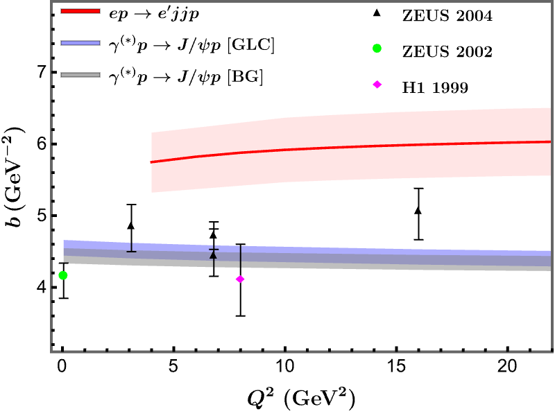
In Fig. 3 (left) the per degree of freedom (dof) as a function of is shown for the case that a fit is made to both the photo- and electroproduction data. It can be seen that also in this case GLC gives a slightly better minimal and prefers a close to the one of the dijet case. Therefore, the GLC model seems to be preferred. However, when it comes to the and slope, all vector meson wave function models require , and values that are smaller than those obtained from the dijet data. This is clearly visible in Fig. 3 (right) where we show the value of of for collisions, where is solely determined by in Eq. (11). The preferred proton profile for the case has fm, while for the dijet case it is fm. Here it should be recalled that the data is for fixed () and the dijet data is integrated () (cf. the bottom right plot of Fig. 1 for the dependence of the dijet data). The slope data points in Fig. 3 (right) are only available for production H1:1999ujo; ZEUS:2004yeh; ZEUS:2002wfj, while the dependence of the dijet slope is extracted from the fit (see Fig. 1). The dijet slope data is given only for and integrated which is . The bands of the slope () for the case shown in Fig. 3 (right) reflect the aforementioned values, while for the dijet case the bands correspond to the error in , i.e. fm, for which a larger gives a larger . Our model shows that the dijet slope is slowly increasing in while for it is steadily decreasing. This tension cannot be resolved with the present set of just three free parameters. It is also clear that it cannot be attributed to the vector meson wave function, but stems from the proton profile. Of course, it may be (in part) due to the aforementioned caveats about the dijet data, but without additional future data, that can likely not be clarified.

In Fig. 4 we show the distribution resulting from the model fits to the -dependence. Both models can describe well the small data (photoproduction). For electroproduction GLC overestimates the data by at most , while BG shows a larger deviation from the data, as shown in Fig. 4 (right).


With the obtained model fits we provide predictions for the same process at EIC, which will cover a different kinematic region, but not so different that evolution will play a big role. The left panel of Fig. 5 shows the predictions without the phenomenological correction and the right panel with. In Fig. 6 we show the correction by itself.


In the left panel of Fig. 6 the correction obtained with the model is plotted for collisions as a function of and found to be in the 10-15% range, a bit larger in the BG model than in the GLC model, and slowly increasing in . This is in agreement with other phenomenological studies Martin:1999wb; Toll:2012mb; Mantysaari:2016jaz. For longitudinal photon polarization a similar size correction is obtained. The right panel shows similar size corrections for UPCs to which we will turn next.


VII Coherent Diffractive Production in UPCs at midrapidity
Ultra-peripheral Heavy Ion Collisions at LHC and RHIC can be used to study photon-nucleus collisions. In order to make sure that one is dealing with exclusive coherent diffractive production of a there need to be rapidity gaps between the and both nuclei. We consider the to be produced at mid-rapidity. The central rapidity range of the LHC is and at RHIC . Here we simply take . In that case the colliding photon and gluon will both have an energy of , which means that the gluon has a momentum fraction of . For the LHC Pb-Pb UPC data ALICE:2021tyx at TeV (Run 2) this corresponds to and at TeV (Run 1) to . For the RHIC Au-Au UPC data at GeV this corresponds to , which is at the edge of the range of applicability of the MV-like model that we are using. We will use the ALICE data to fit and then obtain predictions for RHIC, keeping in mind this caveat.
In order to compare the UPCs to the photoproduction case at EIC, it is useful to know what is in the UPCs. For A-A UPCs at mid-rapidity (), the photon-nucleon center of mass energy squared is determined by Mantysaari:2017dwh. For LHC Pb-Pb UPC data at TeV this corresponds to GeV and at TeV to GeV, while for RHIC Au-Au UPC data at GeV this corresponds to GeV.
In Fig. 7 we provide a fit of our model to the dependence of the differential cross section ALICE:2021tyx for coherent diffractive production at in ultra-peripheral Pb-Pb collisions at TeV. According to ALICE:2021tyx, various models can describe the ALICE data well. One such model is the leading-twist approximation (LTA) of nuclear shadowing Frankfurt:2011cs; Guzey:2016qwo, which combines the Glauber-Gribov formalism with the phenomenology of photon diffraction from HERA. The lower bound of the GLC fit in our model is close to the LTA (low shadowing) model result with a slightly steeper slope, as shown in Fig. 7 (right). Another model, the b-BK Cepila:2020xol; Bendova:2019psy; Bendova:2020hbb, was proposed based on the solution of the Balitsky-Kovchegov equation Balitsky:1995ub; Kovchegov:1999yj with an impact parameter dependence. Another study that incorporates nucleon shape fluctuations Mantysaari:2022sux also provides a good fit to the data, including the coherent dependence of the photoproduction total cross section and the distribution of coherent and incoherent photoproduction data from HERA. While the former two models utilize the BG wave function, our model provides a better description of the and dependence data using the GLC wave function. Another wave function model based on the Buchmüller-Tye potential Buchmuller:1980su that uses - correlation Kopeliovich:2021dgx with two different parameterizations: GBW Golec-Biernat:1998zce; Golec-Biernat:1999qor and BGBK Bartels:2002cj, also gives good agreement with the data Kopeliovich:2022jwe. Differences in the magnitude and slope of the cross section between other models and ours could also be due to the use of different nuclear radius parameters.
Extrapolating the fit gives a prediction of the first diffractive minimum (or dip) to be at . We find that the dip position is determined by the target profile , such that it will move towards a smaller value for larger . The fit turns out to be very sensitive not only to the value of , but also to the power of . With the fit of the model to the ALICE data, we find that for GLC and for BG give the best fit. Therefore, our model fit indicates that the saturation scale behaves like , not . The latter in fact does not provide a good fit. Following Eq. (16), the saturation scale for the heavy nucleus depends on , , and , and is in all cases found to be between 1.5 and 1.9 . The choice of proton and nuclear profile, particularly the Gaussian profile used in our study, can affect the fitted value and may differ with different profiles. We did not attempt to find profiles that would lead to and do not exclude that that is possible.


With the same parameterization, in Fig. 8 we provide predictions for RHIC and LHC (Run 1) at midrapidity. In general, both wave function models give very similar results but GLC shows a somewhat larger band than BG as expected from the previous analysis on (see the in Fig. 3). The left panel in Fig. 8 is for Au-Au UPCs at GeV. Fig. 8 shows that the first diffractive dip for Au-Au at RHIC is predicted to be around which is close to its location in RHIC preliminary data Adam2020 and other studies Cepila:2017nef; Mantysaari:2017dwh, while for Pb-Pb at LHC Run 1 it is predicted to be around . The middle panel in Fig. 8 is for Pb-Pb UPCs at LHC Run 1 with TeV. In the rightmost panel of Fig. 8, we provide predictions of -Au collisions at the EIC for photoproduction () and electroproduction () for fixed which corresponds to and , respectively. The bands for each wave function model reflect the uncertainties on (which translates to ) and . As shown in Fig. 6, the corrections are in the order of 6-10% for UPCs, which is small compared to the uncertainties, hence not included here.


VIII Discussion and Conclusions
We have shown that incorporating dependence in our previous gluon GTMD model, along the lines of the GBW parameterization of the saturation scale, will improve the description of HERA-H1 diffractive dijet production data. However, describing diffractive production in the same way leads to tension for the slope of the dependence, which is quite distinct for the two processes, where dijet needs a steeper slope than production. In the model this slope is solely determined by the (Gaussian) proton profile and there appears to be no clear way to resolve the tension. A few other differences between the optimal parameter choices for dijet and production are found, but these can be reduced by adjusting the wave function or by modifying the dependence w.r.t. the GBW parameterization. For instance, dijet production can be described well by an dependence of the saturation scale with , while the dependence of photoproduction of ’s prefers a smaller . A non-constant may be needed, but we did not explore that option, anticipating that future more precise data may shed new light on the differences between dijet and production. We do expect that a common gluon GTMD model description of dijet and production may be possible once the slope issue is clarified by new data.
With the best fit of our model to combined H1 and ZEUS data on production, we have provided predictions for the diffractive production in - collisions at the future EIC. We further fit our model to UPC data from ALICE (Run 2) to determine the dependence of the saturation scale. The fit turns out to be very sensitive to the power of and the nuclear profile , which suggests that also the profile function shape will matter considerably. We find an dependence that is slightly less than the generally expected , to be specific, . With the obtained fit we provide predictions for UPCs at LHC (Run 1) and RHIC, and for -Au collisions at EIC. We have also investigated a phenomenological correction commonly used for production which comes from the odderon contribution, which is in the 10-15% range and thus unimportant given the present large uncertainties in the available data and hence in the model. The larger correction from accounting for non-zero skewness that is often considered in GPD approaches in the DGLAP regime does not seem appropriate for our GTMD model and was thus not included. Moreover, a similar correction has not been applied in dijet production, which would affect the comparison. We have also pointed out that dijet and production go beyond probing GPDs, rather they probe weighted integrals of GTMDs with weights that depend on external kinematical variables of the process that can be varied and exploited.
The predictions from the presented -dependent gluon GTMD model for production at EIC, LHC, and RHIC, will hopefully facilitate resolution of the distribution tension with dijet production, clarify the dependence on the skewness probed in the process, and determine the and dependence of the saturation scale of heavy nuclei.
Acknowledgements.
We thank Gerco Onderwater for useful discussions on the fits and Cristina Sánchez Gras on the LHCb data. We thank the Center for Information Technology of the University of Groningen for their support and for providing access to the Peregrine high performance computing cluster. The work of C.S. was supported by the Indonesia Endowment Fund for Education (LPDP).References
- (1) Y. Hatta, B. W. Xiao and F. Yuan, Phys. Rev. Lett. 116, no.20, 202301 (2016).
- (2) H. Mäntysaari, N. Mueller and B. Schenke, Phys. Rev. D 99, no.7, 074004 (2019).
- (3) D. Boer and C. Setyadi, Phys. Rev. D 104, no.7, 074006 (2021).
- (4) H. Kowalski, L. Motyka and G. Watt, Phys. Rev. D 74, 074016 (2006).
- (5) D. Bendova, J. Cepila and J. G. Contreras, Phys. Rev. D 99, no.3, 034025 (2019).
- (6) Y. Hatta, B. W. Xiao and F. Yuan, Phys. Rev. D 95, no.11, 114026 (2017).
- (7) H. Mäntysaari, K. Roy, F. Salazar and B. Schenke, Phys. Rev. D 103, no.9, 094026 (2021).
- (8) C. J. Bomhof, P. J. Mulders and F. Pijlman, Eur. Phys. J. C 47, 147-162 (2006).
- (9) D. Boer, T. Van Daal, P. J. Mulders and E. Petreska, JHEP 07, 140 (2018).
- (10) J. Collins,“Foundations of perturbative QCD,” Camb. Monogr. Part. Phys. Nucl. Phys. Cosmol. 32, 1-624 (2011).
- (11) V. Bertone, Eur. Phys. J. C 82, no.10, 941 (2022).
- (12) F. Dominguez, B. W. Xiao and F. Yuan, Phys. Rev. Lett. 106, 022301 (2011).
- (13) F. Dominguez, C. Marquet, B. W. Xiao and F. Yuan, Phys. Rev. D 83, 105005 (2011).
- (14) D. Boer, M. G. Echevarria, P. J. Mulders and J. Zhou, Phys. Rev. Lett. 116, no.12, 122001 (2016).
- (15) K. J. Golec-Biernat and M. Wüsthoff, Phys. Rev. D 59, 014017 (1998).
- (16) K. J. Golec-Biernat and M. Wüsthoff, Phys. Rev. D 60, 114023 (1999).
- (17) A. M. Stasto, K. J. Golec-Biernat and J. Kwiecinski, Phys. Rev. Lett. 86, 596-599 (2001)
- (18) C. Marquet and L. Schoeffel, Phys. Lett. B 639, 471-477 (2006)
- (19) F. Gelis, R. B. Peschanski, G. Soyez and L. Schoeffel, Phys. Lett. B 647, 376-379 (2007)
- (20) F. Caola and S. Forte, Phys. Rev. Lett. 101, 022001 (2008)
- (21) A. Freund, K. Rummukainen, H. Weigert and A. Schafer, Phys. Rev. Lett. 90, 222002 (2003)
- (22) A. H. Mueller, B. W. Xiao and F. Yuan, Phys. Rev. Lett. 110, no.8, 082301 (2013).
- (23) B. W. Xiao, F. Yuan and J. Zhou, Nucl. Phys. B 921, 104-126 (2017).
- (24) J. Zhou, Phys. Rev. D 99, no.5, 054026 (2019).
- (25) D. X. Zheng and J. Zhou, JHEP 11, 177 (2019).
- (26) L. D. McLerran and R. Venugopalan, Phys. Rev. D 49 (1994) 2233.
- (27) L. D. McLerran and R. Venugopalan, Phys. Rev. D 49 (1994) 3352.
- (28) L. D. McLerran and R. Venugopalan, Phys. Rev. D 50 (1994) 2225.
- (29) Y. Hagiwara, Y. Hatta and T. Ueda, Phys. Rev. D 94, no.9, 094036 (2016)
- (30) Y. Hagiwara, Y. Hatta, R. Pasechnik, M. Tasevsky and O. Teryaev, Phys. Rev. D 96, no.3, 034009 (2017)
- (31) F. Salazar and B. Schenke, Phys. Rev. D 100, no.3, 034007 (2019).
- (32) Y. Hatta, E. Iancu, K. Itakura and L. McLerran, Nucl. Phys. A 760, 172-207 (2005).
- (33) E. Iancu and A. H. Rezaeian, Phys. Rev. D 95 (2017) no.9, 094003.
- (34) H. Mäntysaari, F. Salazar and B. Schenke, Phys. Rev. D 106, no.7, 074019 (2022)
- (35) F. D. Aaron et al. [H1], Eur. Phys. J. C 72, 1970 (2012).
- (36) H. Abramowicz et al. [ZEUS Collab.], Eur. Phys. J. C 76 (2016) no.1, 16.
- (37) M. Diehl, Phys. Rept. 388, 41-277 (2003).
- (38) G. Watt and H. Kowalski, Phys. Rev. D 78, 014016 (2008)
- (39) D. Bendova, J. Cepila, J. G. Contreras and M. Matas, Phys. Lett. B 817, 136306 (2021).
- (40) J. Nemchik, N. N. Nikolaev and B. G. Zakharov, Phys. Lett. B 341, 228-237 (1994).
- (41) J. Nemchik, N. N. Nikolaev, E. Predazzi and B. G. Zakharov, Z. Phys. C 75, 71-87 (1997).
- (42) H. Mäntysaari and P. Zurita, Phys. Rev. D 98, 036002 (2018).
- (43) J. Cepila, J. Nemchik, M. Krelina and R. Pasechnik, Eur. Phys. J. C 79, no.6, 495 (2019)
- (44) H. Kowalski and D. Teaney, Phys. Rev. D 68, 114005 (2003)
- (45) B. Z. Kopeliovich and B. G. Zakharov, Phys. Rev. D 44, 3466-3472 (1991)
- (46) E. Eichten, K. Gottfried, T. Kinoshita, K. D. Lane and T. M. Yan, Phys. Rev. D 21, 203 (1980)
- (47) E. Eichten, K. Gottfried, T. Kinoshita, K. D. Lane and T. M. Yan, Phys. Rev. D 17, 3090 (1978) [erratum: Phys. Rev. D 21, 313 (1980)]
- (48) C. Quigg and J. L. Rosner, Phys. Lett. B 71, 153-157 (1977)
- (49) N. Barik and S. N. Jena, Phys. Lett. B 97, 265-268 (1980)
- (50) W. Buchmuller and S. H. H. Tye, Phys. Rev. D 24, 132 (1981)
- (51) V. M. Braun and D. Y. Ivanov, Phys. Rev. D 72, 034016 (2005).
- (52) A. Aktas et al. [H1], Eur. Phys. J. C 46, 585-603 (2006).
- (53) T. Altinoluk, N. Armesto, G. Beuf and A. H. Rezaeian, Phys. Lett. B 758, 373-383 (2016).
- (54) S. Chekanov et al. [ZEUS], Nucl. Phys. B 695, 3-37 (2004).
- (55) A. D. Martin, M. G. Ryskin and T. Teubner, Phys. Rev. D 62, 014022 (2000).
- (56) T. Lappi and H. Mantysaari, Phys. Rev. C 83, 065202 (2011)
- (57) J. Cepila, J. G. Contreras and M. Krelina, Phys. Rev. C 97, no.2, 024901 (2018).
- (58) J. Cepila, J. G. Contreras, M. Krelina and J. D. Tapia Takaki, Nucl. Phys. B 934, 330-340 (2018)
- (59) V. Guzey and M. Zhalov, JHEP 10, 207 (2013)
- (60) V. P. Goncalves, B. D. Moreira and F. S. Navarra, Phys. Rev. C 90, no.1, 015203 (2014)
- (61) S. Zhang, S. Cai, W. Xiang, Y. Cai and D. Zhou, Chin. Phys. C 45, no.7, 073110 (2021)
- (62) K. J. Eskola, C. A. Flett, V. Guzey, T. Löytäinen and H. Paukkunen, Phys. Rev. C 106, no.3, 035202 (2022)
- (63) N. Armesto and A. H. Rezaeian, Phys. Rev. D 90, no.5, 054003 (2014).
- (64) H. Mäntysaari, Rept. Prog. Phys. 83, no.8, 082201 (2020)
- (65) V. N. Gribov and A. A. Migdal, Yad. Fiz. 8, 1213 (1968) & Sov. J. Nucl. Phys. 8 (1969) 703
- (66) A. G. Shuvaev, K. J. Golec-Biernat, A. D. Martin and M. G. Ryskin, Phys. Rev. D 60, 014015 (1999).
- (67) T. Toll and T. Ullrich, Phys. Rev. C 87, no.2, 024913 (2013).
- (68) H. Mäntysaari and B. Schenke, Phys. Rev. D 94, no.3, 034042 (2016)
- (69) C. A. Flett, S. P. Jones, A. D. Martin, M. G. Ryskin and T. Teubner, Phys. Rev. D 101, no.9, 094011 (2020).
- (70) C. Adloff et al. [H1], Phys. Lett. B 483, 23-35 (2000)
- (71) S. Chekanov et al. [ZEUS], Eur. Phys. J. C 24, 345-360 (2002)
- (72) B. Abelev et al. [ALICE], Phys. Lett. B 718, 1273-1283 (2013)
- (73) R. Aaij et al. [LHCb], JHEP 10, 167 (2018)
- (74) R. Aaij et al. [LHCb], J. Phys. G 41, 055002 (2014)
- (75) C. Adloff et al. [H1], Eur. Phys. J. C 10, 373-393 (1999)
- (76) S. Acharya et al. [ALICE], Phys. Lett. B 817, 136280 (2021).
- (77) J. Adam, “Measurements of quarkonia photoproduction in Ultra-Peripheral Collisions at RHIC,” Quarkonia as Tools 2020 workshop.
- (78) H. Mäntysaari and B. Schenke, Phys. Lett. B 772, 832-838 (2017).
- (79) V. Guzey, M. Strikman and M. Zhalov, Phys. Rev. C 95, no.2, 025204 (2017)
- (80) L. Frankfurt, V. Guzey and M. Strikman, Phys. Rept. 512, 255-393 (2012)
- (81) J. Cepila, J. G. Contreras and M. Matas, Phys. Rev. C 102, no.4, 044318 (2020)
- (82) D. Bendova, J. Cepila, J. G. Contreras and M. Matas, Phys. Rev. D 100, no.5, 054015 (2019)
- (83) I. Balitsky, Nucl. Phys. B 463, 99-160 (1996)
- (84) Y. V. Kovchegov, Phys. Rev. D 60, 034008 (1999)
- (85) B. Z. Kopeliovich, M. Krelina and J. Nemchik, Phys. Rev. D 103, no.9, 094027 (2021)
- (86) J. Bartels, K. J. Golec-Biernat and H. Kowalski, Phys. Rev. D 66, 014001 (2002)
- (87) B. Z. Kopeliovich, M. Krelina, J. Nemchik and I. K. Potashnikova, Phys. Rev. D 105, no.5, 054023 (2022)