Spatially Covariant Lesion Segmentation
Abstract
Compared to natural images, medical images usually show stronger visual patterns and therefore this adds flexibility and elasticity to resource-limited clinical applications by injecting proper priors into neural networks. In this paper, we propose spatially covariant pixel-aligned classifier (SCP) to improve the computational efficiency and meantime maintain or increase accuracy for lesion segmentation. SCP relaxes the spatial invariance constraint imposed by convolutional operations and optimizes an underlying implicit function that maps image coordinates to network weights, the parameters of which are obtained along with the backbone network training and later used for generating network weights to capture spatially covariant contextual information. We demonstrate the effectiveness and efficiency of the proposed SCP using two lesion segmentation tasks from different imaging modalities: white matter hyperintensity segmentation in magnetic resonance imaging and liver tumor segmentation in contrast-enhanced abdominal computerized tomography. The network using SCP has achieved 23.8%, 64.9% and 74.7% reduction in GPU memory usage, FLOPs, and network size with similar or better accuracy for lesion segmentation.
1 Introduction
Convolutional neural networks (CNNs) have been the dominant approach across a variety of medical image computing applications such as magnetic resonance imaging (MRI) reconstruction Zhang et al. 2020c; Zhang et al. 2021b, brain lesion segmentation Zhang et al. 2021a; Zhang et al. 2019a, disease identification Khosla et al. 2019; Zhang et al. 2022, and low-dose CT denoising Wang et al. 2022; Fan et al. 2019. Two main properties Elsayed et al. 2020 of CNNs are believed to be the key to their success: 1) The local receptive field increases as the network goes deeper Huang et al. 2017; He et al. 2016, providing richer contextual information for down-stream tasks; 2) Spatially invariant convolution filters regularize the network training, serving as a good inductive bias for grid-based image data Simoncelli and Olshausen 2001. However, medical images scanned from human body exhibit stronger patterns than natural images and therefore the question of whether the spatial invariance is overly restrictive in certain clinical applications remains to be answered.

In contrast to natural images, a large portion of medical images depict human organs through non-invasive imaging techniques such as magnetic resonance imaging (MRI), and these images exhibit more structured patterns than natural images due to their shared similarities across the cohort. Taking the human brain as an example, while brains from different subjects differ in size, disease type or other personal characteristics, all these brains have shown similar hierachical tissue structures across the cohort, e,g., the location and shape of ventricles, white matter and cortex (see Fig. 1). However, most of existing studies on lesion segmentation apply CNN architectures that are originally designed for natural image segmentation, leading to the the structural information loss. From three reproducible observations on brain lesion segmentation we present in the following, we hypothesize that imposing spatial invariance throughout all layers of these CNN architectures is overly restrictive on lesion segmentation tasks with clear tissue structures, and such invariance can be relaxed to improve the computational efficiency and meantime maintain or increase segmentation accuracy to suit needs for resource-limited clinical applications.
Our first observation is that, for CNN-based methods, lesions near cortices or ventricles in human brain are more prone to be mis-segmented than those surrounded by the normal-appearing white matter (NAWM) Moll et al. 2011 in between ventricles and cortex. As shown in Fig. 1, lesions inside the white matter (WM) show more consistent image contrast and tissue structures than those near cortices and ventricles. The change of the context may in part accounts for the mis-segmentation and this raises a question about whether applying the spatially invariant convolution filters is overly restrictive. Second, lesions locate diversely among different individuals but the pattern of the lesion density distribution from a patient cohort are rather structured. As can be seen from Fig. 2, there is a higher lesion density at the peri-ventricular area of the brain, and roughly the lesion density decreases with the distance from the ventricle. Third, the effective receptive field of each pixel differs in its location, where pixels closer to the brain center (inner) have a larger receptive field than those farther away (outer), because the outer ones aggregate more zero values than the inner ones due to the existence of a brain boundary.

In general, better performance can be achieved by enlarging the network size to accommodate changes of the tissue context, lesion density distribution, and receptive field; however, simple enlargement of the network without considering domain-specific information may suffer from a higher computational cost or even overfitting due to the limited amount of medical data. To test our hypothesize, a viable way is replacing the sharing filters with spatially covariant filters. However, this is not applicable as it adds up a huge amount of computational resources, deviating from our original intention. Therefore in this paper, we propose spatially covariant pixel-aligned classifier (SCP) to improve the computational efficiency and meantime maintain or increase accuracy for lesion segmentation. SCP relaxes the spatial invariance constraint imposed by convolutional operations and optimizes an underlying implicit function that maps image coordinates to network weights, the parameters of which are obtained along with the backbone network training and later used for generating network weights to capture spatially variant contextual information. SCP is intriguingly simple and can be plugged into most existing segmentation networks.
We apply SCP to two lesion segmentation tasks, white matter hyperintensity (WMH) segmentation in magnetic resonance imaging (MRI) and liver tumor (LiT) segmentation in contrast-enhanced abdominal computerized tomography (CT), to verify our hypothesis. The main findings of the paper are in three folds: 1) Relaxing spatial variance for tasks with datasets having structured representation or spatially inhomogeneous features are beneficial. 2) SCP works better for WMH segmentation than LiT segmentation as brains are more structured than liver across different individuals. 3) The experimental results suggest that with SCP relaxing the spatial invariance to a certain degree, 23.8%, 64.9% and 74.7% reduction in GPU memory usage, FLOPs, and network parameter size can be achieved without compromising any segmentation accuracy.
2 Related Works
2.1 Lesion Segmentation Networks
Lesion segmentation is one of the most important and difficult tasks in clinical applications, because lesions such as WMH and LiT vary greatly in terms of shape, size, and location. Numerous automated approaches have been proposed to handle the problem, and usually, methods with prior information injected perform better than those using plain neural networks. The Tiramisu network Zhang et al. 2019b uses 2.5D stacked DenseNet Huang et al. 2017 to capture broader brain structural information, Aslani et al. 2019 uses multi-branch residual network He et al. 2016 to fuse multi-contrast information, and Zhang et al. 2019a; Zhang et al. 2020b applies regularized self-attention networks for aggregation of richer contextual information. nnU-Net Isensee et al. 2021 takes one step further to condense and automate the key decisions for designing a successful segmentation network. Despite their success, little domain-specific structure for the network has been developed by these methods, which may lead to sub-optimal results.
The distance transformation mapping has been integrated into neural networks through the development of edge-aware loss functions Kervadec et al. 2019; Zhang et al. 2020a; Karimi and Salcudean 2019 and network layers with anatomical coordinates as prior information Zhang et al. 2021a, improving lesion segmentation performance. These edge-aware loss functions reduces the class imbalance between teh background and lesions, helping segmenting small lesions. Interestingly, All-Net Zhang et al. 2021a has outperformed its pioneers Zhang et al. 2019b; Aslani et al. 2019; Isensee et al. 2021 and achieved the state-of-the-art performance on multiple sclerosis lesion segmentation by explicitly integrating domain-specific information into the neural network. All these methods have achieved a reasonably good result, and we make one step further to provide the possibility and elasticity to find a better trading-off between the segmentation accuracy and computation efficiency by relaxing spatial invariance.
2.2 Invariant Representations of CNNs
While few efforts have been made to study the spatial invariance of CNNs in the context of medical images, many researchers has explored this in natural images. One line of works seek to learn invariant Yi et al. 2016; Cheng et al. 2016; Liu et al. 2019 or equivariant representations Cohen and Welling 2016; Esteves et al. 2018; Esteves et al. 2018; Tai et al. 2019 for CNNs. The performance gain from these methods is usually accompanied with linearly scaled computational cost. Another line of works exploits the hidden information behind the invariant representations learned from CNNs, and our SCP falls in this line. The most related work to our SCP is a low-rank locally connected (LRLC) layer Elsayed et al. 2020 that can parametrically adapt the spatial invariance degree for each convolotion layer by controlling its rank parameter; however, it’s non-trivial to adapt LRLC for lesion segmentation and there is no apparent way of finding a trading-off between accuracy and computation efficiency. Interestingly, Kayhan and Gemert 2020 empirically shows that CNNs consisting of spatially invariant filters can naturally encode absolute spatial location information, reducing the translation invariance in CNNs, and a removal of such encoding can impose stronger inductive bias on the translation invariance, benefiting image classification tasks with small datasets. Further, Islam et al. 2020 analyzes how much spatial information CNNs encode and how CNNs encode, particularly the authors show that the zero-padding near the image border is the key to deliver the spatial location information; however, this implicit spatial information comes at the price of using deeper CNNs or larger convolution filters.
Kayhan and Gemert 2020 and Islam et al. 2020 show that some part of the CNN capacity is occupied by implicit spatial location encoding, meaning that it is possible to preserve this part of capacity for feature learning by feeding directly the spatial location information such as coordinates Liu et al. 2018 to the network. In addition, considering the hierachical structure, boundary shape and spatially inhomogeneous contrast features of human brain, our proposed SCP can further exploit these information and reduce computational complexity.
3 Methodology
3.1 Preliminaries
Let be an input feature map with channels ( and denote the input size, and is the number of input channels), be the feature vector at location , and ( is the number of segmentation categories) be the output of the segmentation head of the network, we can then describe the output logit at position as follows:
| (1) |
where is the trainable weight of the filters for the segmentation head and transforms the feature vector in every location in an identical way using . The spatial invariance refers to sharing the same set of filters across all spatial locations. Usually a practical implementation of Eq. (1) for an encoder-decoder network is a convolution layer, which can be written as follows:
| (2) |
where , and .
3.2 Spatially Covariant Segmentation Head
Let ( is the number of elements for the encoded position vector) be the position encoding tensor, to relax the spatial invariance, we can replace the shared with a function of location:
| (3) |
where is the generated spatially covariant weight, is the trainable parameter for function . Basically, function takes in an encoded position vector and uses its parameter determined by to generate weights for convolution filters. With Eq. (3), we can derive the spatially covariant segmentation head as follows:
| (4) |
Eq. (4) can be seen as a generalization of Eq. (1), as the former reduces to the latter when equals and outputs the regardless of the location information. Thus, by optimizing the function to generate spatially covariant weights across all locations, the spatial invariance is relaxed.

3.3 Position Encoding
Let be an output feature map with channels from a encoder-decoder network, we encode the position at of as follows:
| (5) |
For the rest of the paper, we will refer to instead of as the pixel location. The Fourier representation Rahaman et al. 2019 of the Cartesian coordinates as adopted by neural scene representation Mildenhall et al. 2020 or Transformer architecture Vaswani et al. 2017 is not adopted, because in our application, the surface of generated filter weights is smooth among adjacent pixels, containing no high-frequency information, and enforcing high-frequency variation introduces noise and degrades performance. Also, please note that we use four distances (i.e. the distance to the left, right, top, and bottom) to represent a pixel coordinate, because the input size of the image may vary among different individuals. Compared to encoding position vector as , our four-distance encoding method helps expand a smoother surface for the implicit function .
3.4 Modeling SCP with Neural Networks
It has been shown that the effective receptive field of a CNN has a Gaussian distribution Luo et al. 2016. Without loss of generality, we hypothesize that feature vector at each position follows a multi-variate Gaussian distribution (the dimension is the number of channels ) as follows:
| (6) |
where and are the corresponding mean vector and covariance matrix in location . While the normal CNN assumes that and stay the same across all spatial locations, we relax this restriction by optimizing an implicit function that maps the pixel location to the parameter space of and as follows:
| (7) |
where represents the implicit mapping function which outputs a continuous parameter space of and to generate spatial covariant filter weights. In practice, we use convolution layers to approximate this continuous parameter space and optimize the weight of along with other network weights to map each location to the corresponding mean vector and covariance matrix.
3.5 Derivation of SCP
It has been shown that deep CNNs can linearize Bengio et al. 2013; Upchurch et al. 2017 the manifold of image features into a globally Euclidean subspace of deep features, meaning that the elements of the deep feature vector have minimal interactions with each other. As the input feature map for SCP has passed through an entire encoder-decoder network, the output of the implicit function can be further simplified. More specifically, the covariance matrix can be reduced to a variance vector . We can can then normalize and output the logit of the feature vector at position as follows:
| (8) | ||||
| (9) |
Where and are estimated from the implicit function with as the trainable parameter, is the output logit at position , and is the weight of the final convolution classifier. Note that as we use Z-score to normalize the input image, there is no bias term for the classifier. To be numerically stable, in practice, we estimate and instead, and the equation for normalization and classification of the feature vectorcan be altered as:
| (10) |
where is the Hadamard product. We have derived the spatially covariant segmentation head using the implicit function in Eq. (10). However, in practice, using Eq. (10) directly may generate unnecessary GPU memory usage due to redundant intermediate computation. Looking closer into Eq. (10), we can reformulate it as:
| (11) |
where the first term in Eq. (11) can be replaced with a single generated by the implicit function directly. The second term in Eq. (13) becomes a scalar, serving as a pixel-wise bias term, but as aforementioned, the bias term is not necessary. Upon removing the bias term, we add one residual term to stabilize the network training, and our SCP is derived as follows:
| (12) | ||||
| (13) |
where is estimated from the implicit function with as the trainable parameter, denotes the weight of the residual convolution, serving as the shared term for pixels across all spatial locations.
3.6 Overall Framework Implementation with SCP
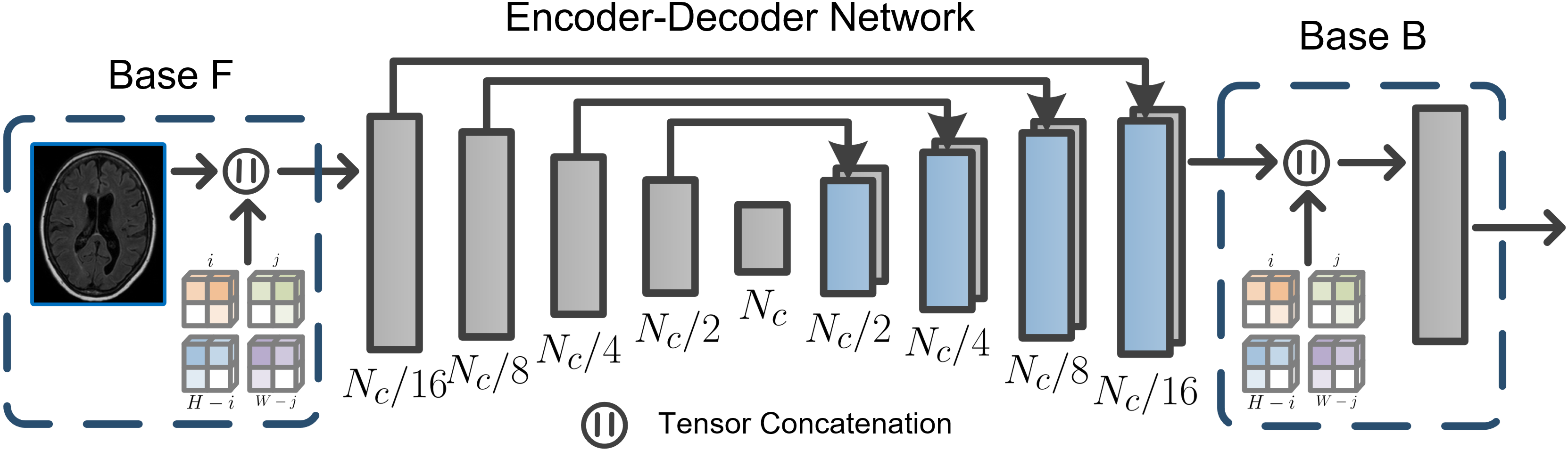
The overall framework consists of an encoder-decoder structured feature extraction network and the proposed SCP module for pixel-wise classification. As shown in Fig. 3, the input image is passed through an encoder-decoder CNN to obtain the intermediate feature map , and in the meantime, pixel-wise position encoding is obtained by concatenating matrices with distances to the left, right, top and bottom of the images. The spatially covariant weight tensor is then generated by the implicit function consisting of two layers of a convolution followed by a ReLU activation function and a single convolution. With for each pixel position, we apply Eq. (13) to output the spatial variant logits for the feature vector of each position. The final segmentation can be obtained by the sum of the output from the residual term and the output from the implicit function, and a Sigmoid function.
| Model | Dice (%) | L-Dice (%) | L-F1 (%) | L-PPV (%) | L-TPR (%) | Memory Ratio | FLOPs Ratio | Parameter Size Ratio | |
|---|---|---|---|---|---|---|---|---|---|
| Base | 128 | 67.41 | 51.53 | 57.53 | 58.48 | 56.62 | 1.00 | 1.00 | 1.00 |
| Base F | 27.94 | 24.41 | 31.91 | 45.25 | 24.64 | 1.06 | 1.02 | 1.00 | |
| Base B | 40.95 | 31.44 | 38.24 | 90.95 | 24.21 | 1.17 | 1.02 | 1.00 | |
| SCP (ours) | 74.47 | 61.30 | 66.39 | 67.28 | 65.53 | 1.78 | 1.42 | 1.02 | |
| Base | 256 | 75.29 | 64.90 | 69.40 | 71.09 | 67.78 | 2.13 | 3.96 | 4.02 |
| Base F | 59.39 | 39.67 | 47.22 | 44.37 | 50.45 | 2.19 | 4.00 | 4.02 | |
| Base B | 67.82 | 56.74 | 64.02 | 83.41 | 51.95 | 2.43 | 4.00 | 4.02 | |
| SCP (ours) | 77.63 | 69.55 | 72.27 | 69.78 | 74.95 | 3.69 | 5.51 | 4.06 | |
| Base | 512 | 75.39 | 65.61 | 70.50 | 67.74 | 73.50 | 4.84 | 15.71 | 16.06 |
| Base F | 62.63 | 45.85 | 54.10 | 54.48 | 53.73 | 4.90 | 15.80 | 16.08 | |
| Base B | 74.90 | 63.89 | 69.97 | 81.67 | 61.20 | 5.39 | 15.82 | 16.08 | |
| SCP (ours) | 77.28 | 70.34 | 73.89 | 75.89 | 72.00 | 7.94 | 21.76 | 16.22 |
4 Experiments and Results
We use PyTorch Paszke et al. 2019 for all network implementations, and train them with an Nvidia RTX 2080Ti GPU. We carefully carry out a set of experiments to show both strengths and useful characteristics of the proposed SCP. We use MRI and CT datasets, which are the most commonly used modalities for medical imaging, to show that SCP generalizes across different imaging techniques. Meanwhile, brain lesions and liver tumors, two commonly seen diseases, are used to demonstrate SCP’s generalization across different human organs.
4.0.1 Baselines and Comparators
All-Net Zhang et al. 2021a is a recently developed network for brain lesion segmentation, outperforming other highly competitive networks such as nnU-Net Isensee et al. 2021, Tiramisu network Zhang et al. 2019b and multi-branch residual network Aslani et al. 2019 on the lesion segmentation task. Without loss of generality, we adopt the backbone network from All-Net as baseline network.
To illustrate the effectiveness of SCP utilizing spatially variant information rather than taking additional coordinates, two network variants with coordinate convolution Liu et al. 2018 are further compared: 1) baseline network with coordinates as an additional input channel (denote as Base F); 2) baseline network with coordinate convolution replacing the final convolution layer (denote as Base B). We also deploy three variants with different model capacity by varing the number of channels in the encoder-decoder network (see Fig. 4 for more details about how changes the network capacity), in which denotes the maximum number of channels in the center layer of the network (e.g. the Base B network with is denoted as Base B (256)).
4.0.2 Evaluation metrics.
To quantify the models’ performance, we use the Dice similarity coefficient Dice 1945, lesion-wise Dice (L-Dice), lesion-wise true positive rate (L-TPR), lesion-wise positive predictive value (L-PPV), and lesion-wise F1 score (L-F1) as metrics. L-Dice, LTPR, and LPPV are defined as , , and , where TPR denotes the number of lesions in ground-truth segmentation that overlap with a lesion in the produced segmentation, and GL, PL are the numbers of lesions in ground-truth segmentation and produced segmentation, respectively. L-F1 is the harmonic mean of L-TPR and L-PPV: . In general, Dice quantifies the voxel-wise overlap between the output and the ground truth, while L-Dice and L-F1 are more sensitive in measuring the lesion-wise detection accuracy. In addition, we use the two-tailed paired t-test to compare Dice and L-Dice metrics for the proposed SCP with other network variants to demonstrate statistical significance for the improved computational efficiency.
4.1 White Matter Hyperintensity Segmentation
Our first experiment is WMH segmentation in human brain. WMH is an important type of brain lesion whose precise tracing can provide useful biomarkers for clinical diagnosis and assessment of disease progression. We use a publicly available 11 1 https://wmh.isi.uu.nl WMH segmentation challenge dataset Kuijf et al. 2019 for our experiments. The dataset contains 60 subjects acquired from different scanners of three institutes. For each subject, a 3D T1-weighted (T1-w) and a 2D multi-slice fluid-attenuated inversion recovery (FLAIR) image are provided. All images are bias-corrected using SPM12 software Ashburner and Friston 2000, followed by co-registering each T1-w image to the FLAIR image. The spatial resolution for each image varies from to , and manual reference segmentation is provided by the consensus of four observers. In the experiments, the dataset is randomly split into three subsets for model training (42), validation (6), and testing (12). The final results of each model are the average of three independent runs with different random seeds (random seed uses the system time and is not sensitive).
4.1.1 Implementation details.
We slice the original volumes into a stack of consecutive images. Each volume is center-cropped to a fixed size of to accommodate batch training, followed by Z-score based intensity normalization. T1-w and FLAIR images of each subject are concatenated through the channel dimension before being used as the input to the network. To train the network, we use Adam Kingma and Ba 2014 optimizer, with an initial learning rate of (weight decay of ), and a batch size of 14. The learning rate is halved at 50%, 70%, and 90% of the total training epoch (90) for optimal convergence.
4.1.2 Quantitative results.
We compare the proposed SCP with the baseline network Zhang et al. 2021a and other variants. Three different levels of network capacities ( for low-capacity, for moderate-capacity, and for high-capacity) of the backbone networks are adopted. Pixel-wise and lesion-wise metric scores as well as ratios of floating point operations per second (FLOPs), memory usage and network parameter size between each network variant and the Base (128) network are shown in Table 1.
In the low-capacity group (), it is observed that SCP (128) outperforms Base (128), Base F (128), and Base B (128) in all metrics except for L-PPV. Though Base B (128) has the highest L-PPV (90.95%), the L-TPR (24.21%) is much lower than SCP (128), resulting in worse L-Dice. Importantly, SCP (128) has at least 7.1% and 9.8% improvement in Dice and L-Dice compared to other network variants with the same compacity. Similar trends in performance are observed among the moderate- and high-capacity groups ( or ), where SCP shows a consistent improvement compared to those networks without the proposed method. Interestingly, both Base F and Base B which take additional coordinate information, perform consistently worse than SCP in all three levels of model capacity, demonstrating the effectiveness of SCP utilizing spatially variant contextual information. In addition, SCP with moderate-capacity backbones achieves better performance compared to other network variants in a higher-capacity backbone. This results in 23.8%, 64.9% and 74.7% reduction in GPU memory usage, FLOPs, and network size respectively without sacrificing any segmentation accuracy.
| Model | Dice (%) | L-Dice (%) | L-F1 (%) | L-PPV (%) | L-TPR (%) | |
|---|---|---|---|---|---|---|
| Base | 128 | 55.57 | 45.76 | 67.29 | 61.20 | 74.73 |
| Base F | 55.13 | 48.76 | 68.65 | 64.84 | 72.94 | |
| Base B | 57.39 | 48.11 | 65.71 | 58.91 | 74.29 | |
| SCP (ours) | 61.21 | 50.13 | 68.03 | 58.90 | 80.50 | |
| Base | 256 | 67.59 | 53.60 | 72.58 | 63.46 | 84.77 |
| Base F | 54.08 | 46.78 | 66.44 | 63.24 | 69.98 | |
| Base B | 69.63 | 50.33 | 67.84 | 56.01 | 86.02 | |
| SCP (ours) | 72.71 | 59.70 | 75.11 | 64.86 | 89.20 | |
| Base | 512 | 71.36 | 48.80 | 67.98 | 54.69 | 89.80 |
| Base F | 56.64 | 48.59 | 65.22 | 55.85 | 78.39 | |
| Base B | 73.33 | 49.15 | 67.57 | 53.82 | 90.75 | |
| SCP (ours) | 73.64 | 49.05 | 66.25 | 52.71 | 89.16 |
4.2 Liver Tumor Segmentation
The second experiment is liver tumor segmentation using images scanned from contrast-enhanced abdominal computerized tomography. It is a challenging task as the image contrast is highly heterogeneous and shape of the liver is diffusive. An open challenge22 2 https://competitions.codalab.org/competitions/17094 dataset LiTS Bilic et al. 2019 from MICCAI 2017 is adopted in our experiment. The dataset is collected from six clinical centers around the world using different scanners and acquisition protocols. There are in total 131 scans, where the in-plane resolution of each scan varies from 0.55 mm to 1.0 mm with a slice spacing ranging from 0.45 mm to 6.0 mm. The horizontal shape of each 3D scan is 512512, and the number of slices varies from 74 to 987. In the image pre-processing step, we truncate the intensity values of each scan to [-200, 250] in order to exclude the non-liver information. Following previous work Ma et al. 2022, we resize the in-plane image from 512512 to 256256. In the experiments, the dataset is split into three subsets for model training (91), validation (13), and testing (27). Similar to the WMH segmentation task, we report the average of three independent runs with different random seeds for each model.
4.2.1 Quantitative results.
As shown in Table 2, we compare SCP with other network variants Base, Base F, and Base B using different network capacities (, or ). Please note that FLOPs, GPU memory usage and network parameter size are excluded in Table 2 because LiTS datasets are trained with the same network as done in WMH. In the low-capacity group (), Base F has a slightly better L-F1 and L-PPV, but the proposed scp improves the Dice and L-Dice scores by 11.0% and 2.8% respectively. SCP (128) has a 5.7% increment for Dice, a 4.4% increment for L-Dice, and a 7.6% increment for L-TPR compared to the Base (128). In addition, SCP (256) consistently outperforms other variants from the moderate-capacity group in terms of Dice and L-Dice. However, similar performance gain as in the WMH segmentation task is not observed in LiTS segmentation in the high-capacity group. Further, the scores of L-F1 and L-Dice are lower in the high-capacity group than those in the moderate-capacity group, indicating that these networks may have encountered overfitting problem.
4.3 Statistical & Complexity Analysis
Paired t-tests are used compare performance metrics of Dice and L-Dice between the proposed SCP (256) and other network variants Base (256), Base (512), Base F (512), Base B (512). SCP (256) from the moderate-capacity group is used to compare other variants from the high-capacity group, because the goal for SCP is to improve computational efficiency and in the meantime maintain or achieve better segmentation accuracy by relaxing the spatial invariance. As we can see from Fig. 5a and Fig. 5b, in WMH segmentation task, except for Base B (512) on Dice, SCP (256) outperforms all other network variants with statistical significance () on both Dice and L-Dice. Fig. 5c and Fig. 5d show that in LiTS segmentation task, SCP outperforms all other network variants in terms of Dice and L-Dice scores; however, SCP (256) only outperforms Base F (512) on Dice and Base (512) and Base B (512) on L-Dice with statistical significance ().
Combining results from paired t-tests and Fig. 6, we can conclude that the proposed SCP (256), relaxing spatial invariance, achieves a significant reduction on computational cost (23.8%, 64.9% and 74.7% reduction in GPU memory usage, FLOPs, and network size) without losing any segmentation accuracy on both WMH and LiTS segmentation tasks. The main advantage achieved by SCP is the computation efficiency, favorably making the image analysis tool more accessible in clinical environments without GPU support.
4.4 Discussions
To understand how SCP relaxes the spatial invariance and how datasets affect the learning of the spatially covariant weight , we have plotted five key statistics of as shown in Fig. 7. To make value color consistent, we use min-max to normalize each statistic image with value ranging from 0 to 1. Please note that as both WMH and LiTS segmentation tasks are binary, is set to 1. From left to right in Fig. 7 are the maximum values, mean values, minimum values, L2-Norm and standard deviation (STD) of along the channel dimension respectively.
As shown in Fig. 7, the weight learned from the WMH segmentation shows a stronger pattern than that learned from the LiTS segmentation, where all five statistics of the weight delineate an average image of the shape of human brain. The statistic images from the LiTS segmentation instead delineate the shape of human breast rather than the target liver. The boundary of the max value map is clearer in WMH than in LiTS, and the value distribution across five statistics is more consistent in WMH than LiTS. Moreover, in the max, min and mean value maps from the WMH, value decreases with distance from the center, and especially in the max value map, there is a clear boundary between averaged brain area and background. The max value map from WMH segmentation shows consistency with the receptive field where pixels closer to the brain center has a larger receptive field than those farther away. However, as the shape and location of human liver varies greatly from patient to patient, such phenomenon is not observed from the LiTS segmentation.
Interestingly, we have found out that SCP is more sensitive to small lesions, and more details and qualitative results can be found in the supplementary materials. In conclusion, SCP can help relax the spatial variance and benefit lesion segmentation tasks with datasets having structured representation or spatially inhomogeneous features, e.g. aligned human brains with hierachical tissue structure.
5 Conclusions
In this paper, we present a novel network module, called spatially covariant pixel-aligned classifier (SCP), to trade-off between computational efficiency and accuracy for lesion segmentation. SCP relaxes the spatial invariance constraint imposed by convolutional operations and optimizes an underlying implicit function that maps image coordinates to network weights, the parameters of which can be obtained along with the backbone network training and later used for generating network weights to capture spatially variant contextual information. We find out that SCP suits lesion segmentation tasks with datasets having structured representation or spatially inhomogeneous features. We believe that the proposed SCP technique will contribute to more medical imaging applications in the future.

References
- Abraham et al. [2014] Alexandre Abraham, Fabian Pedregosa, Michael Eickenberg, Philippe Gervais, Andreas Mueller, Jean Kossaifi, Alexandre Gramfort, Bertrand Thirion, and Gaël Varoquaux. Machine learning for neuroimaging with scikit-learn. Frontiers in neuroinformatics, page 14, 2014.
- Ashburner and Friston [2000] John Ashburner and Karl J Friston. Voxel-based morphometry—the methods. Neuroimage, 11(6):805–821, 2000.
- Aslani et al. [2019] Shahab Aslani, Michael Dayan, Loredana Storelli, Massimo Filippi, Vittorio Murino, Maria A Rocca, and Diego Sona. Multi-branch convolutional neural network for multiple sclerosis lesion segmentation. NeuroImage, 196:1–15, 2019.
- Bengio et al. [2013] Yoshua Bengio, Grégoire Mesnil, Yann Dauphin, and Salah Rifai. Better mixing via deep representations. In International conference on machine learning, pages 552–560. PMLR, 2013.
- Bilic et al. [2019] Patrick Bilic, Patrick Ferdinand Christ, Eugene Vorontsov, Grzegorz Chlebus, Hao Chen, Qi Dou, Chi-Wing Fu, Xiao Han, Pheng-Ann Heng, Jürgen Hesser, et al. The liver tumor segmentation benchmark (lits). arXiv preprint arXiv:1901.04056, 2019.
- Cheng et al. [2016] Gong Cheng, Peicheng Zhou, and Junwei Han. Learning rotation-invariant convolutional neural networks for object detection in vhr optical remote sensing images. IEEE Transactions on Geoscience and Remote Sensing, 54(12):7405–7415, 2016.
- Cohen and Welling [2016] Taco S Cohen and Max Welling. Steerable cnns. arXiv preprint arXiv:1612.08498, 2016.
- Dice [1945] Lee R Dice. Measures of the amount of ecologic association between species. Ecology, 26(3):297–302, 1945.
- Elsayed et al. [2020] Gamaleldin Elsayed, Prajit Ramachandran, Jonathon Shlens, and Simon Kornblith. Revisiting spatial invariance with low-rank local connectivity. In International Conference on Machine Learning, pages 2868–2879. PMLR, 2020.
- Esteves et al. [2018] Carlos Esteves, Christine Allen-Blanchette, Ameesh Makadia, and Kostas Daniilidis. Learning so (3) equivariant representations with spherical cnns. In Proceedings of the European Conference on Computer Vision (ECCV), pages 52–68, 2018.
- Fan et al. [2019] Fenglei Fan, Hongming Shan, Mannudeep K Kalra, Ramandeep Singh, Guhan Qian, Matthew Getzin, Yueyang Teng, Juergen Hahn, and Ge Wang. Quadratic autoencoder (q-ae) for low-dose ct denoising. IEEE transactions on medical imaging, 39(6):2035–2050, 2019.
- Fischl [2012] Bruce Fischl. Freesurfer. Neuroimage, 62(2):774–781, 2012.
- He et al. [2016] Kaiming He, Xiangyu Zhang, Shaoqing Ren, and Jian Sun. Deep residual learning for image recognition. In Proceedings of the IEEE conference on computer vision and pattern recognition, pages 770–778, 2016.
- Huang et al. [2017] Gao Huang, Zhuang Liu, Laurens Van Der Maaten, and Kilian Q Weinberger. Densely connected convolutional networks. In Proceedings of the IEEE conference on computer vision and pattern recognition, pages 4700–4708, 2017.
- Isensee et al. [2021] Fabian Isensee, Paul F Jaeger, Simon AA Kohl, Jens Petersen, and Klaus H Maier-Hein. nnu-net: a self-configuring method for deep learning-based biomedical image segmentation. Nature methods, 18(2):203–211, 2021.
- Islam et al. [2020] Md Amirul Islam, Sen Jia, and Neil DB Bruce. How much position information do convolutional neural networks encode? In International Conference on Learning Representations, 2020.
- Karimi and Salcudean [2019] Davood Karimi and Septimiu E Salcudean. Reducing the hausdorff distance in medical image segmentation with convolutional neural networks. IEEE Transactions on medical imaging, 39(2):499–513, 2019.
- Kayhan and Gemert [2020] Osman Semih Kayhan and Jan C van Gemert. On translation invariance in cnns: Convolutional layers can exploit absolute spatial location. In Proceedings of the IEEE/CVF Conference on Computer Vision and Pattern Recognition, pages 14274–14285, 2020.
- Kervadec et al. [2019] Hoel Kervadec, Jihene Bouchtiba, Christian Desrosiers, Eric Granger, Jose Dolz, and Ismail Ben Ayed. Boundary loss for highly unbalanced segmentation. In International conference on medical imaging with deep learning, pages 285–296. PMLR, 2019.
- Khosla et al. [2019] Meenakshi Khosla, Keith Jamison, Amy Kuceyeski, and Mert R. Sabuncu. Ensemble learning with 3d convolutional neural networks for functional connectome-based prediction. NeuroImage, 199:651–662, 2019.
- Kingma and Ba [2014] Diederik P Kingma and Jimmy Ba. Adam: A method for stochastic optimization. arXiv preprint arXiv:1412.6980, 2014.
- Kuijf et al. [2019] Hugo J Kuijf, J Matthijs Biesbroek, Jeroen De Bresser, Rutger Heinen, Simon Andermatt, Mariana Bento, Matt Berseth, Mikhail Belyaev, M Jorge Cardoso, Adria Casamitjana, et al. Standardized assessment of automatic segmentation of white matter hyperintensities and results of the wmh segmentation challenge. IEEE transactions on medical imaging, 38(11):2556–2568, 2019.
- Liu et al. [2018] Rosanne Liu, Joel Lehman, Piero Molino, Felipe Petroski Such, Eric Frank, Alex Sergeev, and Jason Yosinski. An intriguing failing of convolutional neural networks and the coordconv solution. In Proceedings of the 32nd International Conference on Neural Information Processing Systems, pages 9628–9639, 2018.
- Liu et al. [2019] Yuan Liu, Zehong Shen, Zhixuan Lin, Sida Peng, Hujun Bao, and Xiaowei Zhou. Gift: Learning transformation-invariant dense visual descriptors via group cnns. Advances in Neural Information Processing Systems, 32, 2019.
- Luo et al. [2016] Wenjie Luo, Yujia Li, Raquel Urtasun, and Richard Zemel. Understanding the effective receptive field in deep convolutional neural networks. Advances in neural information processing systems, 29, 2016.
- Ma et al. [2022] Tianyu Ma, Adrian V Dalca, and Mert R Sabuncu. Hyper-convolution networks for biomedical image segmentation. In Proceedings of the IEEE/CVF Winter Conference on Applications of Computer Vision, pages 1933–1942, 2022.
- Mildenhall et al. [2020] Ben Mildenhall, Pratul P Srinivasan, Matthew Tancik, Jonathan T Barron, Ravi Ramamoorthi, and Ren Ng. Nerf: Representing scenes as neural radiance fields for view synthesis. arXiv preprint arXiv:2003.08934, 2020.
- Moll et al. [2011] Natalia M Moll, Anna M Rietsch, Smitha Thomas, Amy J Ransohoff, Jar-Chi Lee, Robert Fox, Ansi Chang, Richard M Ransohoff, and Elizabeth Fisher. Multiple sclerosis normal-appearing white matter: Pathology–imaging correlations. Annals of neurology, 70(5):764–773, 2011.
- Paszke et al. [2019] Adam Paszke, Sam Gross, Francisco Massa, Adam Lerer, James Bradbury, Gregory Chanan, Trevor Killeen, Zeming Lin, Natalia Gimelshein, Luca Antiga, et al. Pytorch: An imperative style, high-performance deep learning library. In Advances in Neural Information Processing Systems, pages 8024–8035, 2019.
- Rahaman et al. [2019] Nasim Rahaman, Aristide Baratin, Devansh Arpit, Felix Draxler, Min Lin, Fred Hamprecht, Yoshua Bengio, and Aaron Courville. On the spectral bias of neural networks. In International Conference on Machine Learning, pages 5301–5310. PMLR, 2019.
- Simoncelli and Olshausen [2001] Eero P Simoncelli and Bruno A Olshausen. Natural image statistics and neural representation. Annual review of neuroscience, 24(1):1193–1216, 2001.
- Tai et al. [2019] Kai Sheng Tai, Peter Bailis, and Gregory Valiant. Equivariant transformer networks. In International Conference on Machine Learning, pages 6086–6095. PMLR, 2019.
- Upchurch et al. [2017] Paul Upchurch, Jacob Gardner, Geoff Pleiss, Robert Pless, Noah Snavely, Kavita Bala, and Kilian Weinberger. Deep feature interpolation for image content changes. In Proceedings of the IEEE conference on computer vision and pattern recognition, pages 7064–7073, 2017.
- Vaswani et al. [2017] Ashish Vaswani, Noam Shazeer, Niki Parmar, Jakob Uszkoreit, Llion Jones, Aidan N Gomez, Łukasz Kaiser, and Illia Polosukhin. Attention is all you need. Advances in neural information processing systems, 30, 2017.
- Wang et al. [2022] Dayang Wang, Fenglei Fan, Zhan Wu, Rui Liu, Fei Wang, and Hengyong Yu. Ctformer: Convolution-free token2token dilated vision transformer for low-dose ct denoising. arXiv preprint arXiv:2202.13517, 2022.
- Yi et al. [2016] Kwang Moo Yi, Eduard Trulls, Vincent Lepetit, and Pascal Fua. Lift: Learned invariant feature transform. In European conference on computer vision, pages 467–483. Springer, 2016.
- Zhang et al. [2019a] Hang Zhang, Jinwei Zhang, Qihao Zhang, Jeremy Kim, Shun Zhang, Susan A Gauthier, Pascal Spincemaille, Thanh D Nguyen, Mert Sabuncu, and Yi Wang. Rsanet: Recurrent slice-wise attention network for multiple sclerosis lesion segmentation. In International Conference on Medical Image Computing and Computer-Assisted Intervention, pages 411–419. Springer, 2019.
- Zhang et al. [2019b] Huahong Zhang, Alessandra M Valcarcel, Rohit Bakshi, Renxin Chu, Francesca Bagnato, Russell T Shinohara, Kilian Hett, and Ipek Oguz. Multiple sclerosis lesion segmentation with tiramisu and 2.5 d stacked slices. In International Conference on Medical Image Computing and Computer-Assisted Intervention, pages 338–346. Springer, 2019.
- Zhang et al. [2020a] Hang Zhang, Jinwei Zhang, Rongguang Wang, Qihao Zhang, Susan A Gauthier, Pascal Spincemaille, Thanh D Nguyen, and Yi Wang. Geometric loss for deep multiple sclerosis lesion segmentation. arXiv preprint arXiv:2009.13755, 2020.
- Zhang et al. [2020b] Hang Zhang, Jinwei Zhang, Rongguang Wang, Qihao Zhang, Pascal Spincemaille, Thanh D Nguyen, and Yi Wang. Efficient folded attention for 3d medical image reconstruction and segmentation. arXiv preprint arXiv:2009.05576, 2020.
- Zhang et al. [2020c] Jinwei Zhang, Zhe Liu, Shun Zhang, Hang Zhang, Pascal Spincemaille, Thanh D Nguyen, Mert R Sabuncu, and Yi Wang. Fidelity imposed network edit (fine) for solving ill-posed image reconstruction. NeuroImage, 211:116579, 2020.
- Zhang et al. [2021a] Hang Zhang, Jinwei Zhang, Chao Li, Elizabeth M. Sweeney, Pascal Spincemaille, Thanh D. Nguyen, Susan A. Gauthier, Yi Wang, and Melanie Marcille. All-net: Anatomical information lesion-wise loss function integrated into neural network for multiple sclerosis lesion segmentation. NeuroImage: Clinical, 32:102854, 2021.
- Zhang et al. [2021b] Hang Zhang, Jinwei Zhang, Rongguang Wang, Qihao Zhang, Pascal Spincemaille, Thanh D Nguyen, and Yi Wang. Efficient folded attention for medical image reconstruction and segmentation. In Proceedings of the AAAI Conference on Artificial Intelligence, volume 35, pages 10868–10876, 2021.
- Zhang et al. [2022] Hang Zhang, Thanh D Nguyen, Jinwei Zhang, Melanie Marcille, Pascal Spincemaille, Yi Wang, Susan A Gauthier, and Elizabeth M Sweeney. Qsmrim-net: Imbalance-aware learning for identification of chronic active multiple sclerosis lesions on quantitative susceptibility maps. NeuroImage: Clinical, 34:102979, 2022.