Distributed Reproduction Numbers of
Networked Epidemics

Let $\underline{n}$ denote the index set $\{1,2,3,\dots,n\}$. For a matrix $\mathcal{A}\in\mathbb{R}^{n\times n}$, we use $[\mathcal{A}]_{ij}$ to denote the $ij^{th}$ entry of $\mathcal{A}$. We use $\rho(\mathcal{A})$ to represent the spectral radius of the matrix $\mathcal{A}$. For a vector $x\in\mathbb{R}^{n}$, we use $\text{diag}(x)\in\mathbb{R}^{n\times n}$ to denote the diagonal matrix with the $i$th diagonal entry being $x_{i}$ for all $i\in\underline{n}$. For two vectors $x,y\in\mathbb{R}^{n}$, we use $x>y$ to denote that there exists at least one $i\in\underline{n}$ such that $x_{i}>y_{i}$. Denote $\boldsymbol{0}$ and $\boldsymbol{1}$ as the zero vector and one vector with the corresponding dimension given by context. Let $[a,b]^{n}$ denote a closed cube and $(a,b)^{n}$ denote an open cube, for any $a,b\in\mathbb{R}$.

The networked $SIS$ and $SIR$ models are popular in modeling and analyzing epidemic spreading processes [7, 8, 9, 10], and we study them throughout the paper. We consider epidemic processes on strongly connected graphs of $n$ communities. For all $i\in\underline{n}$, let $s_{i}$, $x_{i}$, and $r_{i}$ represent the susceptible, infected, and recovered proportions of the population of community $i$, respectively. We use $s_{i}(t)$ and $s_{i}$ interchangeably. The classic networked $SIS$ model is

and the classic networked $SIR$ model is

In these models, $\beta_{ij}\geq 0$ denotes the transmission rate from community $j$ to community $i$ for all $i,j\in\underline{n}$, and ${\gamma_{i}>0}$ denotes the recovery rate of community $i$ for all $i\in\underline{n}$. Further, we define $\mathcal{B}\in\mathbb{R}^{n\times n}_{\geq 0}$ such that $[\mathcal{B}]_{ij}=\beta_{ij}$ for all $i,j\in\underline{n}$ as the transmission matrix. We define the diagonal matrix $\mathcal{D}\in\mathbb{R}^{n\times n}_{\geq 0}$ such that $[\mathcal{D}]_{ii}=\gamma_{i}>0$ for all $i\in\underline{n}$ as the recovery matrix.

Note that at an endemic equilibrium one cannot have $x^{*}_{i}=0$ or $x_{i}^{*}=1$ for any $i\in\underline{n}$ [7]. Inspired by the use of reproduction numbers to construct threshold conditions for the analysis of non-networked epidemic models, researchers have studied the spreading behaviors of the networked $SIS$ and $SIR$ models in (1) and (2) using thresholds conditions [7, 8, 9, 10]. These threshold conditions are defined in terms of the reproduction numbers of networks (namely the network-level reproduction numbers).

Further, we can leverage both reproduction numbers of networks in Definition 2 to characterize the spreading behaviors of the network, illustrated by the following two lemmas.

It is less useful to analyze the existence of equilibria of the networked $SIR$ model, since $SIR$ models have an infinite number of healthy equilibria but cannot have any endemic equilibria. Instead, we are more interested in studying the transient behavior of the $SIR$ model. Thus, we use $w$ to denote the normalized left eigenvector of the matrix $\mathcal{D}-\mathcal{B}$, and the following lemma summarizes the transient behavior of the networked $SIS$ and $SIR$ models.

Note that the original theorems [7, Thm. 4.2, 4.3] and [7, Thm. 5.2, 5.4] capture the case of homogeneous transmission rates in a network. However, the results for heterogeneous transmission networks listed in Lemma 1 and Lemma 2 can be obtained through the similar proofs given by [7, Thm. 4.2, 4.3] and [7, Thm. 5.2, 5.4].

Lemma 1 and Lemma 2 characterize the spreading behaviors of the networked models in (1) and (2) through the reproduction numbers of the network, i.e., $R^{0}$ and $R^{t}$. However, these reproduction numbers of the network may fail to capture the spreading behavior of individual entities within the network. To illustrate this point, Fig. 1 presents the infected proportion of each community in a networked $SIR$ model over ten communities in a strongly connected graph. The dashed line indicates $w^{\top}x$. Fig. 2 shows the corresponding effective reproduction number of the network, i.e., $R^{t}$. The effective reproduction number $R^{t}>1$ until roughly timestep $20$. However, the infected proportions of most communities, including $x_{1}$, $x_{2}$, and $x_{6}$, already start decreasing by timestep $20$.

Therefore, if we aim to analyze an individual community or a subnetwork of connected communities within the network, the reproduction numbers of the network, $R^{0}$ and/or $R^{t}$, may fail to capture the spreading behavior, since both thresholds in Lemmas 1 and 2 characterize network-level spreading only.

Motivated by this discussion of the reproduction numbers of networks, we formulate the following problem statements.

We will answer Questions 1-3 in the next two sections.

One way to study epidemic spreading processes is to leverage reproduction numbers to indicate the change of the infected population (e.g., increasing, decreasing, unchanging.). As indicated in Lemmas 1 and 2, network-level reproduction numbers can capture the overall spreading behavior within a network. However, the spreading behavior of an individual community might not be captured by the reproduction numbers of the network. Thus, based on the intuition that the infected population of community $i$ will increase if the effective reproduction number of community $i$ is greater than $1$, and vice versa, we introduce the following definition of distributed reproduction numbers.

In order to explain the intuition behind Definition 3, we consider the group compartmental $SIS$ and $SIR$ models with $\beta$ and $\gamma$ being the transmission and recovery rates, respectively [7]. Note that the two models admit $\frac{\beta}{\gamma}$ and $\frac{s(t)\beta}{\gamma}$ as the basic and effective reproduction numbers, respectively. Based on these terms, we then choose to use $R^{0}_{ij}=\frac{\beta_{ij}}{\gamma_{i}}$ and $R^{t}_{ij}=\frac{s_{i}(t)\beta_{ij}}{\gamma_{i}}$ for the basic and pseudo-effective reproduction numbers of the infected proportion $x_{ij}$, where $x_{ij}$ denotes the infected proportion in community $i$ generated by the infected proportion in community $j$ for all $i,j\in\underline{n}$. Through the definition, we have $\frac{dx_{ij}}{dt}>0$ if and only if $R^{t}_{ij}>1$, and vice versa. Further, we define the scaled infected proportion $\bar{x}_{ij}=x_{ij}I_{ij}$ for all $i,j\in\underline{n}$. Note that the scaled infected proportion $\bar{x}_{ij}$ can be considered as a normalized infected proportion of $\bar{x}_{ij}$ with respect to community $i$. When computing effective reproductions of community $i$, it is necessary to evaluate the infections from different resources at the same scale. The following lemma shows the use of $\bar{R}^{t}_{ij}=R^{t}_{ij}I_{ij}$.

Based on Lemma 3, the pseudo-effective reproduction numbers together with the infection ratios, i.e., $\bar{R}^{t}_{ij}=R^{t}_{ij}I_{ij}$, are used as the effective reproduction number from community $j$ to community $i$ for all $i,j\in\underline{n}$. The basic reproduction number captures the situation where $s_{i}\approx 1$ for all $i\in\underline{n}$, and the effective reproduction number captures cases in which $x_{i}\in(0,1]$ for all $i\in\underline{n}$. Definition 3 proposes distributed reproduction numbers by separating the infected cases generated in community $i$ in two ways: (i) the new cases that are generated through the infected cases within the community itself, and (ii) the new cases that are generated through the infected cases from neighboring communities. Hence, we use two types of reproduction numbers, namely the reproduction numbers within a community ($R^{0}_{ii}$ and $R^{t}_{ii}$) and the reproduction numbers from one community to another community ($R^{0}_{ij}$ and $\bar{R}^{t}_{ij}$), to capture the two types of infection processes. In addition, similar to the reproduction numbers of group compartmental models, we have $R^{t}_{ii}=s_{i}R^{0}_{ii}$ within community $i$ for all $i\in\underline{n}$. For the pseudo-effective reproduction numbers from community $j$ to $i$, we have $R^{t}_{ij}=s_{i}R^{0}_{ij}$ for all $i,j\in\underline{n}$.

Definition 3 and Lemma 3 propose a way of explaining spread processes through the distributed reproduction numbers within and between communities. For the purpose of characterizing the spread process of a community, we further define the basic reproduction number and effective reproduction number of a community within the network, through the distributed reproduction numbers in Definition 3.

Through the distributed reproduction numbers introduced in Definition 3 and Lemma 3, we can compose the reproduction numbers of an individual community through the sum of the distributed reproduction numbers, as shown in Definition 4. Compared to the effective reproduction number of the network ($R^{t}$), the effective reproduction number of an individual community ($\bar{R}^{t}_{i}$) can facilitate the study of the spreading behavior of community $i$ for all $i\in\underline{n}$.

Theorem 1 demonstrates that the definition of the effective reproduction numbers exhibits thresholding behavior, and thus that we can leverage the effective reproduction numbers of communities to capture the spreading behavior within and between them. In addition, recall that the effective reproduction number of the whole network, $R^{t}$, is monotonically non-increasing, since for all $i\in\underline{n}$, the value of $s_{i}$ is monotonically non-increasing [7]. However, for all $i\in\underline{n}$ the value of $\bar{R}_{i}^{t}$ can be non-monotonic.

Theorem 1, Lemma 3, and Lemma 4 demonstrate that we can leverage the distributed reproduction numbers to capture spreading behaviors of individual communities. Hence, we have answered Question 1 from Section II. In order to answer Question 2, we connect distributed reproduction numbers to the network-level reproduction numbers of networks, namely $R^{0}$ and $R^{t}$. First we define the distributed reproduction number matrices.

Based on Definition 2, it can be observed that $\mathcal{R}^{0}=\mathcal{D}^{-1}\mathcal{B}$ and $\mathcal{R}^{t}=\text{diag}(s)\mathcal{D}^{-1}\mathcal{B}$. Hence, the spectral radius of the distributed basic reproduction number matrix, denoted $\rho(\mathcal{R}^{0})$, is the basic reproduction number of the network, i.e., $\rho(\mathcal{R}^{0})=R^{0}$. Meanwhile, the spectral radius of the distributed effective reproduction number matrix, denoted $\rho(\mathcal{R}^{t})$, is the effective reproduction number of the network, i.e., $\rho(\mathcal{R}^{t})=R^{t}$. Further, for all $i\in\underline{n}$, the $i^{th}$ row sum of the distributed basic reproduction number matrix is the reproduction number of community $i$, i.e., we have $\sum_{j=1}^{n}[\mathcal{R}^{0}]_{ij}=R^{0}_{i}$. Note that the $i^{th}$ row sum of the distributed effective reproduction number matrix, $\mathcal{R}^{t}$, is not equal to $R_{i}^{t}$, since the weights $I_{ij}$ are not included in $\mathcal{R}^{t}$.

Through studying the spreading behavior of the network, we connect the effective reproduction number of the network to the effective reproduction numbers of the communities.

Using Theorem 2 and Lemma 1, we can characterize the spreading behaviors of the $SIS$ and $SIR$ models through $\bar{R}^{t}_{i}$.

Lemmas 1 and 2 indicate that if $R^{0}<1$, then the weighted sum of the infected states will converge to zero. However, unlike the fact that $R^{t}\leq R^{0}$ for network-level reproduction numbers, if the basic reproduction number of community $i$ is less than $1$ for all $i\in\underline{n}$, then the effective reproduction number of community $i$ can still be greater than $1$. Hence, we have the following corollary.

After demonstrating that we can use the distributed reproduction numbers to analyze spreading behaviors, we showed that the distributed reproduction numbers are closely related to the basic and effective reproduction numbers of the network in Theorem 2, Corollary 1, and Corollary 2. Hence we have answered Question 2 that not only can we use the distributed reproduction numbers to analyze spreading behaviors of individual entities within the network, but also we can use the distributed reproduction numbers to study the overall spreading behavior of the network as a whole.

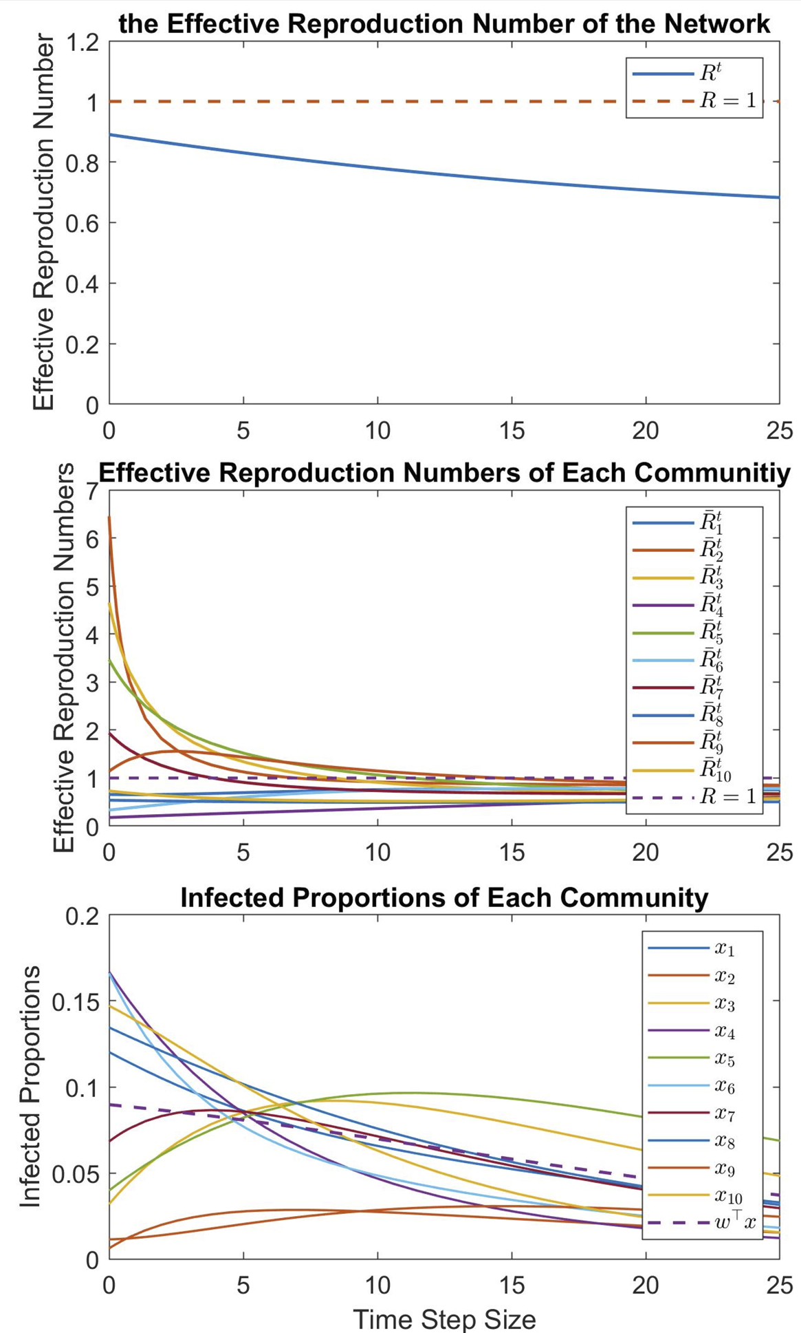
Consider an epidemic spreading over ten strongly connected communities, as shown in Fig. 3. Suppose the epidemic spreads based on the classic networked $SIR$ models in (2). We capture the spreading behavior in the plots in Fig. 4. Fig. 4 (Top) shows that the effective reproduction number of the whole network ($R^{t}$) is always less than $1$. Thus, if a community uses this $R^{t}$ for policy-making and forecasting, then the community might believe that the infected proportion of the population will decrease from time step zero.

However, there are still outbreaks over several communities, e.g., communities 3 and 5 in Fig. 4 (Bottom), where the infected proportions in fact increase for several timesteps at the beginning. These outbreaks can be explained through the distributed reproduction numbers of the communities, which are plotted in Fig. 4 (Middle). Through analyzing Fig. 4 (Middle), $\bar{R}^{t}_{3}$ and $\bar{R}^{t}_{5}$ are greater than $1$ at the beginning, which indicate outbreaks within them and thus that both communities should take actions against potential outbreaks. This simple case demonstrates that it is more informative to leverage distributed reproduction numbers when designing mitigation policies for individual community.

In the second example, we show how we can calculate distributed reproduction numbers from synthetic data to analyze spreading over a network, which completes our answer to Question 3 from Section II. We construct a piece-wise time-varying stochastic $SIR$ spreading process over the strongly connected 3-node network shown in Fig. 5.

Suppose each community has a population of $20,000$. We set the initial infected population of communities 1, 2, and 3 as 12, 3, and 23, respectively. We assume the spread occurs from $2020-03-03$ to $2020-06-02$. For the daily infected cases, we assume that we know the total infected cases and the sources which cause these infections (e.g., new infections caused within a community or caused by neighbors). We use the method proposed by [16] to estimate the distributed effective reproduction numbers defined in this work, where a statistical inference approach is used and the estimation only relies on daily infected cases.

Fig. 6 (Top) shows the total daily infected cases of the three connected communities. We estimated the effective reproduction number of the network $R^{t}$, given in Fig. 6 (Bottom). The estimated $R^{t}$ can illustrate that the total infected cases start to decrease around $2020-04-10$, since $R^{t}<1$ after that date. However, the estimated $R^{t}$ in Fig. 6 cannot provide any further information about the spreading behaviors of the individual communities.

In order to study the spreading behavior of each community, we leverage the daily infected cases of each community to estimate the effective reproduction number of each community, denoted $\bar{R}^{t}_{i}$ for $i\in\underline{3}$. We plot the infected cases of each community, shown in Fig. 7 (Top). Further, we plot the estimated effective reproduction numbers of communities 1, 2, and 3 ($\bar{R}^{t}_{1}$, $\bar{R}^{t}_{2}$, and $\bar{R}^{t}_{3}$) in Fig. 7 (Bottom three). As shown by $\bar{R}^{t}_{1}\approx 1$ between $2020-03-24$ to $2020-04-21$, the daily infected cases of community $1$ remain unchanged. Meanwhile, according to $\bar{R}^{t}_{3}$ from $2020-03-17$ to $2020-03-24$, it is possible for the outbreak in community 3 to become worse, since $\bar{R}^{t}_{3}>1$ and $\bar{R}^{t}_{3}$ is increasing. Hence, compared to $R^{t}$ in Fig. 6, $\bar{R}^{t}_{i}$ for $i\in\underline{3}$ can give more specific insights about individual communities.

Last, given the assumption that we know the cause of the infections of the communities (either generated by the infected cases within the community or the infected cases from its neighbors), we can leverage the infected cases generated by the neighbors (Fig. 8 (Top)) to estimate the distributed pseudo-effective reproduction numbers $R^{t}_{ij}$. As shown in Fig. 8 (Bottom Middle), through observing the distributed reproduction number $R^{t}_{21}$, we find that $R^{t}_{21}\approx 1$ from $2020-03-31$ to $2020-05-05$. This observation indicates that the daily infections in community $2$ that are introduced from the infected population in community $1$ remain unchanged. Thus, if we want to further decrease the infections in community $2$ generated by community $1$, we can implement a mitigation strategy that restricts interactions between these two communities and monitor $R^{t}_{21}$ as an indicator of the effectiveness of the strategy. For further indications, according to $R^{t}_{13}$ in Fig. 8 (Top Middle), $R^{t}_{13}>1$ from $2020-03-10$ to $2020-03-17$, then $R^{t}_{13}<1$ from $2020-03-17$ to $2020-03-24$. One can infer that the interaction from communities $3$ to $1$ may vary drastically from $2020-03-10$ to $2020-03-24$, due to the implementation of mitigation policies between these communities, e.g. traffic restrictions from $2020-03-17$ to $2020-03-24$.

References

- [1] P. van den Driessche, “Reproduction numbers of infectious disease models,” Infec. Dise. Model., vol. 2, no. 3, pp. 288–303, 2017.
- [2] K. Soltesz, F. Gustafsson, T. Timpka, J. Jaldén, C. Jidling, A. Heimerson, T. B. Schön, A. Spreco, J. Ekberg, Ö. Dahlström et al., “The effect of interventions on COVID-19,” Nature, vol. 588, no. 7839, pp. E26–E28, 2020.
- [3] B. She, J. Liu, S. Sundaram, and P. E. Paré, “On a networked epidemic model with cooperative and antagonistic opinion dynamics,” IEEE Trans, on Contr. of Netw. Syst., vol. 9, pp. 1154 – 1165, 2022.
- [4] B. Pascal, P. Abry, N. Pustelnik, S. Roux, R. Gribonval, and P. Flandrin, “Nonsmooth convex optimization to estimate the Covid-19 reproduction number space-time evolution with robustness against low quality data,” IEEE Trans. on Sig. Proc., vol. 70, pp. 2859–2868, 2022.
- [5] K. D. Smith and F. Bullo, “Convex optimization of the basic reproduction number,” arXiv preprint arXiv:2109.07643, 2021.
- [6] F. Casella, “Can the COVID-19 epidemic be controlled on the basis of daily test reports?” IEEE Control Syst. Letters, vol. 5, no. 3, pp. 1079–1084, 2020.
- [7] W. Mei, S. Mohagheghi, S. Zampieri, and F. Bullo, “On the dynamics of deterministic epidemic propagation over networks,” Annu. Rev. in Control, vol. 44, pp. 116–128, 2017.
- [8] P. E. Paré, C. L. Beck, and T. Başar, “Modeling, estimation, and analysis of epidemics over networks: An overview,” Annu. Rev. in Control, vol. 50, pp. 345–360, 2020.
- [9] L. Zino and M. Cao, “Analysis, prediction, and control of epidemics: A survey from scalar to dynamic network models,” IEEE Cir. and Syst. Mag., vol. 21, no. 4, pp. 4–23, 2021.
- [10] C. Nowzari, V. M. Preciado, and G. J. Pappas, “Analysis and control of epidemics: A survey of spreading processes on complex networks,” IEEE Control Syst. Magazine, vol. 36, no. 1, pp. 26–46, 2016.
- [11] P. Van Mieghem, “The N-intertwined SIS epidemic network model,” Computing, vol. 93, no. 2, pp. 147–169, 2011.
- [12] J. Liu, P. E. Paré, A. Nedić, C. Tang, C. Beck, and T. Başar, “Analysis and control of a continuous-time bi-virus model,” IEEE Trans. Autom. Control, vol. 64, no. 12, pp. 4891–4906, 2019.
- [13] “Modeling COVID-19 scenarios for the United States,” Nature Medicine, vol. 27, no. 1, pp. 94–105, 2021.
- [14] O. Diekmann, J. Heesterbeek, and M. G. Roberts, “The construction of next-generation matrices for compartmental epidemic models,” J. of the Roy. Soc. Inter., vol. 7, no. 47, pp. 873–885, 2010.
- [15] R. S. Varga, Matrix Iterative Analysis. Springer Science & Business Media, 2009, vol. 27.
- [16] A. Cori, N. M. Ferguson, C. Fraser, and S. Cauchemez, “A new framework and software to estimate time-varying reproduction numbers during epidemics,” Amer. J. of Epi., vol. 178, no. 9, pp. 1505–1512, 2013.