Standing and Traveling Waves in a Model of Periodically Modulated One-dimensional Waveguide Arrays
Abstract
In the present work, we study coherent structures in a one-dimensional discrete nonlinear Schrödinger lattice in which the coupling between waveguides is periodically modulated. Numerical experiments with single-site initial conditions show that, depending on the power, the system exhibits two fundamentally different behaviors. At low power, initial conditions with intensity concentrated in a single site give rise to transport, with the energy moving unidirectionally along the lattice, whereas high power initial conditions yield stationary solutions. We explain these two behaviors, as well as the nature of the transition between the two regimes, by analyzing a simpler model where the couplings between waveguides are given by step functions. For the original model, we numerically construct both stationary and moving coherent structures, which are solutions reproducing themselves exactly after an integer multiple of the coupling period. For the stationary solutions, which are true periodic orbits, we use Floquet analysis to determine the parameter regime for which they are spectrally stable. Typically, the traveling solutions are characterized by having small-amplitude, oscillatory tails, although we identify a set of parameters for which these tails disappear. These parameters turn out to be independent of the lattice size, and our simulations suggest that for these parameters, numerically exact traveling solutions are stable.
I Introduction
The study of nonlinear lattice dynamics has been fundamental in advancing our understanding of light propagation in nonlinear optics Lederer et al. 2008 and the wavefunction properties of atomic condensates Morsch and Oberthaler 2006, among others. In the former realm, the relevant models consider the propagation of light in coupled arrays of optical waveguides, while in the latter setting, they explore the evolution of the mean-field wavefunction in the context of deep optical lattices. In both scenarios, the universal model of interest (also considered as an envelope wave model in other discrete settings, including mechanical and electrical lattices Remoissenet 1999; Dauxois and Peyrard 2006) has been the prototypical discrete nonlinear Schrödinger (DNLS) lattice Kevrekidis 2009.
Progressively, over the past few years, a topic that has been gaining significant traction has been the exploration of topological features in both linear and nonlinear systems exhibiting wave dynamics. Indeed, recent studies in a diverse host of fields including, but not limited to, photonics Ozawa et al. 2019, phononics Ma et al. 2019; Süsstrunk and Huber 2016, metamaterials Deng et al. 2021, and atomic physics Cooper et al. 2019, highlight unique dynamical properties resulting from the interplay of nonlinearity and topology. Relevant realizations of, e.g., SSH lattice systems and associated anomalous edge states have also been recently proposed in the work of Zhou et al. 2022 with the potential of application in the context of topoelectrical metamaterials. Notably, their interplay has been leveraged to produce solitonic excitations and domain walls Lumer et al. 2013; Solnyshkov et al. 2017; Smirnova et al. 2019; Marzuola et al. 2019; Mukherjee and Rechtsman 2020; Chen et al. 2014; Hadad et al. 2017; Poddubny and Smirnova 2018, and to generate robust states propagating on domain edges Ablowitz et al. 2014; Leykam and Chong 2016; Kartashov and Skryabin 2016; Snee and Ma 2019; Tao et al. 2020 that defy discreteness-induced barriers such as the famous Peierls-Nabarro barrier Ablowitz et al. 2021. The resulting “topologically protected” states achieve unidirectional, uninhibited propagation around lattice defects in topological lattices Ablowitz and Cole 2019. These intense recent efforts have been summarized, e.g., in Smirnova et al. 2020; Ma et al. 2021, and also in the very recent and detailed review of Ablowitz and Cole 2022.
Among the many ongoing efforts in the field of topological photonics, we single out here a series of highly influential recent experiments of Rechtsman and collaborators Mukherjee and Rechtsman 2020; Mukherjee and Rechtsman 2021; Jürgensen and Rechtsman 2022; Jürgensen et al. 2021. Topological photonics has its roots in two seminal 2008 papers Haldane and Raghu 2008; Raghu and Haldane 2008, where the authors delineated in detail the one-on-one correspondence between condensed matter physics (CMP) and photonics. In particular, the propagation direction plays the role of time in the original CMP setting, and hence leads to a notion of “pseudo-time”. For the same reason the conjugate wave-number is referred to as a “pseudo-frequency” (). The first of these works Mukherjee and Rechtsman 2020 showcased the experimental realization of Floquet solitons in a topological bandgap, the numerical existence and stability of which we subsequently explored in Parker et al. 2022. More recently, such dispersive nonlinear systems with a coupling dependent on the evolution variable were proposed as a suitable realization of nonlinear Thouless pumps Jürgensen and Rechtsman 2022, and the topological properties of the bands such as the Chern number were argued to govern the resulting soliton motion. In Jürgensen et al. 2021, the analogy with the quantum Hall effect and the original proposal of the Thouless pump Thouless 1983 was taken further by studying how nonlinearity acts to quantize transport via soliton formation and spontaneous symmetry-breaking bifurcations. In the present work, influenced by these studies, we consider the system analyzed in Jürgensen et al. 2021, but we depart from the adiabatic regime of focus in that work. By doing so, we are able to capture topologically induced stationary and dynamic states beyond the adiabatic approximation. We do so by enabling the computation of numerically exact stationary solutions, but importantly also traveling solutions. Not only do we generate such waveforms by “generic” dynamical evolution experiments, but we also study a simple variant of the model which considers piecewise-constant coupling strengths (in a way reminiscent of the celebrated Kronig-Penney model Kronig and Penney 1931). There, it becomes evident that at a qualitative level, the transition between standing and traveling waves mirrors the self-trapping transition of the DNLS dimer Kenkre and Campbell 1986. The latter may provide a quite relevant insight towards understanding the symmetry breaking transitions and dynamics within the intensely studied topic of nonlinear Thouless pumps.
Our findings are structured as follows. In Section II, we present the theoretical setup and our quantitative diagnostics used in the model of interest. In Section II.2, we rescale the model so that we can use the propagation distance as a parameter. We subsequently turn to numerical computations in Section III, starting with the evolution of single-site initial conditions, and then gaining insights from the simplified piecewise-constant coupling model. In Section III.1, we perform evolution experiments which demonstrate that there are two fundamental behaviors to the system. For low initial power, the initial intensity moves either to the left or to the right in the lattice. The direction of motion depends on the lattice site chosen for the initial condition. For high initial power, the intensity remains confined to a single lattice site. In addition, there does not appear to be a sharp transition between these two behaviors when the starting intensity of the single site is continuously varied. In Section III.2, we consider a simplification of the model in which the coupling between waveguides is given by step functions. An analysis of this simplified model for an optical dimer explains these two observed behaviors, as well as the lack of a sharp transition between them. In Section III.3, we numerically construct both stationary and traveling coherent structures. As opposed to what occurs with single-site initial conditions, these coherent structures reproduce themselves exactly after an integer multiple of the coupling period. We use Floquet theory to determine the spectral stability of the stationary coherent structures, which are periodic orbits of the system. Finally, in section IV we summarize our findings and present our conclusions, including a number of directions for future study.
II Theoretical Analysis
II.1 Mathematical Model
As discussed above, and motivated by experiments such as those of Jürgensen and Rechtsman 2022; Jürgensen et al. 2021, we study light propagation in an array of coupled optical waveguides, where the coupling is periodically modulated along the axis of light propagation. Mathematically, this is described by the non-autonomous variant of the DNLS model of the form
| (1) |
where is the complex amplitude of light propagating at the waveguide in the lattice site indexed , is the propagation distance (in the direction along the waveguides), and is the linear, -dependent (i.e., dependent on the evolution variable) tight-binding Hamiltonian, or equivalently the lattice coupling profile. It is important to clarify here that the non-autonomous nature of the system under study is in connection with the notion of pseudo-time (corresponding to the propagation distance) as indicated above. It is with that sense of non-autonomy in mind that we will proceed hereafter. The parameter quantifies the strength of the cubic Kerr nonlinearity. For , as in Jürgensen et al. 2021, we use an off-diagonal implementation of the Aubry-André-Harper model Aubry and André 1980; Harper 1955 with three sites per unit cell, resulting in the model
| (2) |
The -dependent coupling functions are periodic in with spatial period , which we will refer to as the coupling period. We note that Jürgensen et al. 2021 considers this model in the adiabatic regime, i.e. for very large (see, for example, (Jürgensen et al. 2021, Figure 2), where ), in which case the system is approximately at a “frozen” equilibrium for every . This is a central point to the analysis presented therein, which is explicitly geared towards (and limited to) such an adiabatic regime. By contrast, the parameter regime we consider herein is that of relatively small , e.g. . In this case, stationary solutions are (genuine) periodic orbits of the system, which, in turn, enables us to use the tools of Floquet analysis to determine their spectral stability.
While we consider larger below (see, in particular, Fig. 14), we note that our methods do not allow us to compute exact periodic orbits for which is very large, i.e. ones which would approach the adiabatic regime (see the end of Section III.3.1 for further details).
The choice of
| (3) |
groups the lattice sites into unit cells comprising three waveguides each (Fig. 1, see also (Jürgensen et al. 2021, Figure 1)), since for . This choice of is (slightly) modified from Equation (3) in the supplement of Jürgensen et al. 2021; squaring the cosine function ensures that the coupling is always positive, which would be the case in a physical realization of the model. We note that if we do not square the cosine (as in the supplement of Jürgensen et al. 2021), thus allowing for negative coupling values, we obtain the same qualitative behavior.

II.2 Model Rescaling and Density Evolution
In order to use the spatial period as a parameter, we rescale the propagation distance using the change of variables so that the coupling period is always 1.
| (5) | ||||
At any propagation distance , the power of the solution is its squared norm
| (6) |
where the sum is taken over the entire lattice. The optical intensity at lattice site is the square amplitude . The power is conserved, i.e., is independent of . Using equation Eq. 5 and its complex conjugate, we derive the flux equations for the density matrix elements
| (7) | ||||
The evolution of the optical intensity (or density) of the solution at lattice site , which is given by , is
| (8) | ||||
where we used the fact that . We can split the last line of Eq. 8 into two components, which we denote
| (9) | ||||
where and are the flow of intensity into site from the left and the right (respectively), and a positive sign indicates that intensity is flowing into site from the labeled neighboring site.
III Numerical Computations
III.1 Single site evolution
As an initial experiment, we consider dynamical simulations starting with a single excited site at . Unless otherwise specified, the parameters in the section are , , , and , and the simulations are run on a finite lattice with lattice points, with periodic boundary conditions on the ends of the lattice (i.e., a ring, which allows for waves to loop around when they reach the boundaries). Evolution in is performed with ode45 in Matlab using a tolerance of . For a single-site initial condition of sufficiently high power (above a threshold between and for input intensity at , and between and for input intensity at ), the energy remains concentrated at a single site, and the resulting excitation appears to be stable (see bottom right panel of Fig. 2 and Fig. 3). We will address the associated slight difference in the power threshold between initial excitations at and below.
As the initial power is lowered, this single-site solution becomes prone to mobility; in both cases, this leads the initially concentrated intensity to leak to the right within the lattice before dispersing throughout the lattice (bottom left panels of Fig. 2 and Fig. 3). For lower power initial conditions (between and ), the initial intensity moves either to the left in the lattice (for initial excited site at , see top of Fig. 2) or to the right (for initial excited site at , see top of Fig. 3) before dispersing through the lattice. One explanation for this observation is as follows: for the first third of the period (), the strongest coupling is between site and via (see Eq. Eq. 3 and Fig. 1), so intensity can flow to the left from to , which occurs when the initial power is sufficiently low. For , the strongest coupling is between and , and for , the strongest coupling is between and , thus we expect the intensity to travel three sites to the left over one period. Similarly, for the rightward moving solution starting at , the rightward coupling is strongest for a rightward sequence of sites on the intervals , , and , thus this solution moves to the right three sites in two periods. A similar rightward moving behavior occurs when the initial excited site is (not shown). The first coupling for is to the right on the interval ; the behavior is then similar to that of the rightward moving solution for . We thus conclude that this fundamental difference between the leftward and rightward moving solutions and the associated speeds is a direct consequence of the form of the periodic coupling function, together with the lattice site at which the initial intensity is placed; this is suggestive also towards the difference in power thresholds noted above. In addition, we believe that this intuitive explanation is quite straightforward and, thus, appealing towards understanding solitary wave motion in such non-autonomous discrete nonlinear systems.


III.2 Simplified model
A further heuristic and qualitative, yet in our view informative and intuitive, explanation of these different behaviors can be obtained by considering the simplification of the system of Eq. 2 obtained by approximating the coupling functions with step functions, as is done, e.g., in the setting of the Kronig-Penney model Kronig and Penney 1931. Note that such a perspective has also been beneficial in a quantitative fashion in the case of nonlinearity (rather than dispersion) management in works such as Centurion et al. 2006a; Centurion et al. 2006b. Specifically, we define
| (10) |
for , and extend periodically for all (Fig. 4). The function is the characteristic function of the interval , defined by

Using this approximation, on the interval , the only active coupling is between the sites and their left neighbors, which effectively creates a string of independent dimers. Our analysis follows Kenkre and Campbell’s study of self-trapping in a DNLS dimer Kenkre and Campbell 1986. Similar to what was done in that work, we will derive a second order differential equation for the difference in intensity between the two sites of the dimer. This ODE will have solutions in terms of Jacobi elliptic functions, and these will be used to explain the observed transition between mobile and trapped solutions as the coupling strength is increased. We note that this allows us to write the intensities (not the complex amplitudes ) in terms of Jacobi elliptic functions.
Looking only at the sites and , i.e., one of these dimers, the system of equations Eq. 8 reduces to the four equations
| (11) | ||||
Let be the difference between the intensities of site and site . As in Kenkre and Campbell 1986, we will derive a second-order ODE for . Following the analysis in Kenkre 1989, we define
| (12) | ||||
Using Eq. 11, we obtain the system of first-order ODEs
| (13) | ||||
| (14) | ||||
| (15) |
Since
equation Eq. 15 becomes
which has solution
| (16) |
where and are the initial conditions for and , respectively, at . Differentiating Eq. 13 and substituting Eq. 14 and Eq. 16, we obtain the second-order differential equation for
| (17) | ||||
This second-order, autonomous differential equation with a linear term and a cubic nonlinearity has an exact solution in terms of Jacobi elliptic functions (See section 22.13(iii) of DLMF as well as Carlson 2006). We are interested in the case of a single-site initial condition with intensity at site , for which and . Following Kenkre and Campbell 1986, for fixed and , equation Eq. 17 has an exact solution
| (18) |
where the critical intensity is given by
| (19) |
The functions and are the Jacobi elliptic functions with elliptic modulus (we note that these are often written in terms of the elliptic parameter , where ). Since the power of the solution is conserved, i.e. , the intensity at sites and on the interval is given by
| (20) | ||||
There are two fundamental behaviors of the single-site initial condition in the simplified model, depending on whether or . In the dimer, a sharp transition between the two behaviors occurs at (see Kenkre and Campbell 1986). We note that this transition is somewhat blurred in this model, even with the simplified coupling function, since the initial dimer coupling is broken () at . Below we will discuss and case-by-case.
III.2.1 Case 1:
For , the solution involves the Jacobi cn function, which oscillates about 0 with period , where
| (21) |
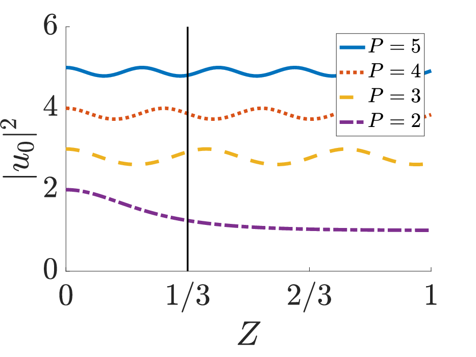
is the complete elliptic integral of the first kind. (We note that the period of oscillation becomes infinite as approaches from below). The intensity , given by equation Eq. 20, exhibits large amplitude oscillations with this period from 0 to , centered at (Fig. 5, left). Intensity initially flows to the left; if the coupling is not cut off at (and no other couplings are activated), there is a critical value of at which the intensity from site has been completely transferred to site ; after this point, intensity starts flowing back in the other direction. This critical value is larger for larger starting intensity (see Fig. 5, left). For most configurations, including all of the examples in Fig. 5, the critical value , thus there is still intensity remaining in site 0 when the coupling switches off at . The left panel of Fig. 6 plots the fraction of intensity that has been transferred from site to site at as the starting intensity varies. If this fraction is close to 1, numerical evolution experiments find leftward-moving solutions starting from a single-site initial condition (see the first three panels of Fig. 7). As the initial intensity approaches from below, the fraction of intensity transferred at decreases to approximately 0.5, and we do not expect to see pure leftward-moving solutions. Numerical evolution experiments in this case show that the initial intensity splits into a leftward and a rightward moving solution (bottom right panel of Fig. 7).
We note that it is possible to choose parameters so that, for the simplified model, the period of is 2/3, i.e. , so that the initial intensity has been completely transferred from to when the coupling switches off. The next coupling is then between and for . This pattern continues, and so for this choice of parameters, the simplified model supports an exact leftward-moving solution which persists for a large interval in (Fig. 8, top). A comparison between the evolution of the original and simplified systems from single-site initial conditions for , illustrating the similarity of the model dynamics, is shown in the top panel of Fig. 9. We will see below in Section III.3.2 that left-moving coherent structures exist in the full model, but these do not have pure single-site initial conditions. We also note that by symmetry of Eq. 11, a similar analysis holds for rightward-moving solutions starting with single-site initial conditions at on the interval .
 |
 |
 |
 |


 |
 |
 |
 |
 |
 |
III.2.2 Case 2:
For , the solution involves the Jacobi dn function, which oscillates about 1 with period , where is defined by Eq. 21. (We again note that the period of oscillation becomes infinite as approaches from above). The intensity exhibits small amplitude oscillations (which become progressively smaller as is increased) with this period about the initial intensity (Fig. 5, right). As in Case 1, the intensity initially flows to the left. If the coupling is not cut off at (and no other couplings are activated), there is a critical value of at which point the system has returned to its initial state, i.e. the intensities at sites and are once again and 0, respectively. For most configurations, including all of the examples in Fig. 5, the critical value , thus when the coupling switches off, there has been some net transfer of intensity to the neighboring site . The right panel of Fig. 6 plots the fraction of intensity remaining at site at for varying . If this fraction is close to 1, numerical evolution simulations show stationary solutions starting from a single-site initial condition; the closer this fraction is to 1, the longer these stationary solutions will persist before breaking up; see the case examples in Fig. 10.
As in Case 1, we note that it is possible to choose parameters so that, for the simplified model, the system returns exactly to its starting condition at , i.e. (Fig. 5, bottom). In this case, for a single-site initial condition with a specific starting intensity, the simplified model supports a localized in space, time-periodic solution which persists for a large interval in . A comparison between the evolution of the original and simplified systems for is shown in the bottom panel of Fig. 9. We discuss genuinely time-periodic (numerically exact) coherent structures in the full model in Subsection Section III.3.1.

III.3 Coherent Structures in the Full Model
These evolution experiments are strongly suggestive of the fact that the system Eq. 5 supports two classes of coherent structures: localized in space, time-periodic solutions, which are centered at a particular lattice site, and moving solutions, which reproduce themselves exactly a specific number of sites to the left or to the right. Recall that for the rescaled system Eq. 5, the coupling period is 1. The stationary coherent structures will be periodic orbits whose period is a multiple of the coupling period, i.e., a positive integer (we refer to this below). We note that while it may be possible to find such solutions which have a non-integer period, Floquet analysis requires that the period of the solutions be commensurate with that of the coupling. Similarly, we will look for moving solutions that reproduce themselves, shifted left or right, after an integer period.
For appropriate choices of system parameters, we can compute both types of solutions numerically. For both localized (i.e., non-moving) and moving solutions, we use a shooting method with periodic boundary conditions imposed on , starting with a single-site initial guess. In addition, for the former case, we validate this method by using numerical parameter continuation with AUTO Doedel et al. 2007 to solve a periodic boundary value problem. Unless otherwise specified, the parameters in the section are the same as in the previous one.
III.3.1 Stationary (non-moving) solutions
First, we look at the stationary solutions. At the anti-continuum (AC) limit ( and ), the lattice sites are decoupled, and an initial intensity at lattice site will yield a standing wave solution of frequency , i.e., of the form . Since such a solution has period , and stationary solutions must have an integer period, these solutions will exist in a discrete family for every integer period , i.e., approximately for sufficiently large positive integer . For period and the parameters in the previous section, for example, we expect to have time-periodic, non-moving solutions for approximate integer intensities . See Fig. 11 and Fig. 12 for the first two of these solutions. By looking at the intensity and the real part of the central site (middle panel), we see that they are approximately standing waves with frequency 2 and 3 (respectively). We note that the stationary solutions do not decay to 0 with increasing , but rather the tails exhibit small amplitude oscillatory patterns (see top right of Fig. 11 and Fig. 12); the specific pattern of oscillations depends on the lattice size (not shown). Looking at the sites adjacent to the central one, the left neighbor peaks on the interval when the coupling is most active, and the leftward flow , indicating flow of intensity out of site 0 to the left. The right neighbor peaks on the interval when the coupling is most active, and the rightward flow , indicating flow of intensity out of site 0 to the right. Both and are close to 0 on the interval , when neither nearest-neighbor coupling is strong.


Since these non-mobile solutions are true periodic orbits with integer period, so that their period is equal to or commensurate with that of the coupling, their spectral stability can be determined by Floquet theory. Numerical computation of the Floquet multipliers of the stationary solutions is shown in the insets of the top left plots in Fig. 11 and Fig. 12. The lower power solution has two pairs of Floquet multipliers off of the unit circle, which is characteristic of an oscillatory instability. Long term evolution in (bottom right plot of Fig. 11) shows that this solution remains coherent until approximately . By contrast, the Floquet spectrum of the higher power solution lies on the unit circle, indicating spectral stability. Long term evolution in (bottom right plot of Fig. 12) shows that this solution is still coherent at .
Using numerical parameter continuation, we start with the DNLS soliton at and slowly vary , tracing the curves in Fig. 13 ( throughout). Since we are looking for solutions with period 1, the starting single site intensity must take integer values so that the frequency of the DNLS standing wave at is commensurate with this period. In all cases, a turning point is reached, as is increased, at which point the parameter continuation in the coupling parameter reverses direction. This turning point occurs at a larger value of for solutions which start at a higher initial intensities at . All stationary solutions initially have their Floquet spectrum confined to the unit circle, thus are spectrally stable. Spectral stability is lost at some point before the turning point observed in the graph, when Floquet multipliers collide and leave the unit circle, creating an oscillatory instability. Solutions on the upper branches of the bifurcation diagram are periodic solutions to the DNLS which are not pure standing waves. To leading order, these upper solutions are the sum of two Fourier modes, as opposed to standing waves, which comprise a single Fourier mode. Substituting the finite Fourier ansatz
into Eq. 5 and projecting onto each of the Fourier basis functions, we can obtain expressions for the coefficients for each wavenumber . An FFT of the numerical solution on the upper branches suggests that the solutions at each site are composed predominantly of the modes with wavenumbers 0 and 1. Thus, to leading order, these solutions are of the form , where the coefficients and satisfy
We note that if for all , the second equation reduces to the DNLS equation, in which case the solution is a standing wave.


We can also continue solutions in the coupling period (Fig. 14). The intensity of the central peak, hence the overall power of the solution, decreases with increasing , thus solutions with greater starting power at persist for higher . For example, solutions with (approximate) starting power of 2, 3, and 4 at persist up to , 15.7, and 16.6, respectively (see Fig. 14). Again, there is a turning point where the continuation reverses directions, which occurs at larger for higher power branches. The central site for the upper and lower branches of each loop has approximately the same intensity; the higher power of the upper branches is due to larger intensity in the tails of the solutions. For contrast, the spatial period of the solutions in (Jürgensen et al. 2021, Figure 2) is , which simulates the adiabatic regime; since the power of the solution decreases as is increased by parameter continuation, we would have to start with a solution with extremely high power at to be able to reach such a large using this method. Obtaining such solutions with a very large spatial period directly by a shooting method is similarly computationally impractical.

Finally, we note that, while we have only considered non-moving solutions with period of 1, stationary solutions do exist for other positive integer periods. For example, if we start with a single-site initial condition with intensity for positive, odd integer , we expect that we will obtain a stationary solution with period 2. (We have verified that this is the case for single-site initial conditions with intensities 3/2 and 5/2). While, in principle, this can be done for any integer period, it becomes computationally intractable for larger periods.
III.3.2 Moving solutions
Next, we look for moving solutions. For a given lattice size , we find that leftward moving solutions exist (Fig. 15) for all values of within an interval (see top right and bottom left of Fig. 16). These are true coherent structures, in that the entire solution reproduces itself exactly after one period, shifted three sites to the left. (In the numerical simulation, where we are using periodic boundary conditions on the lattice, we can think of this as a “circular shift”). We note that is possible to find solutions which reproduce themselves modulo a phase multiplier after one period, and these will have different power from the true coherent structures; we will not consider these solutions herein. Generically, these solutions have oscillatory tails (Fig. 15, top right), and the amplitude of these oscillations depends on the lattice size (Fig. 16, top left). Notice, however, that the corresponding wavenumber in the far field does not. At a critical value of ( for and ), the tail oscillations vanish, leaving a localized traveling solution (Fig. 16, bottom right). Most notably, the value of is independent of the lattice size , although it does depend on both and (Fig. 17). The left moving solution appears to be stable when (see Fig. 20, left); at minimum, it persists unchanged for at least 1000 periods. In addition, the solution appears to be stable for an interval in containing (not shown). The presence of seems to suggest an analogy with the so-called Stokes constant calculation in similar traveling (DNLS-type) problems, as in the work of Oxtoby and Barashenkov 2007. Further expanding on this connection could be an interesting problem for the future (but is outside the scope of the present work). Since the traveling solution is not a periodic orbit, we cannot use standard Floquet analysis to determine its spectral stability. That being said, since the traveling solution is periodic modulo a shift by an integer number of lattice points, it might be possible to adapt some aspects of Floquet theory to this case. We note that while the parameter continuation in the bottom left of Fig. 16 continues past the turning points at and (so that there are solutions with different powers for the same value of ), this merely represents growth of the tail oscillations, while the intensity of the central site remains essentially unchanged; since none of these solutions are stable, the continuation diagram is not shown past these turning points.
Similar results are obtained for the right-moving solutions (Fig. 18 and Fig. 19). Once again, the tail oscillations vanish at a critical value of ( for and ), which is close, but not equal, to the value for the left-moving solution. The right-moving solution also appears to be stable at (and near) (see Fig. 20, right). Unlike the left-moving solution, which is symmetric (Fig. 15, top left), the right-moving solution is asymmetric (Fig. 18, top left). For the initial condition of the right-moving solution, the intensity profile is skewed to the right. In addition, the intensity of the central site for the right-moving solution (approximately 0.6842) is significantly higher than that of the left-moving solution (approximately 0.3416).


III.4 Collisions
Finally, we briefly explore the resulting phenomenology when a left-moving and a right-moving solution collide, an event shown in Fig. 21. For the relevant initial condition, we splice together well-separated copies of the left-moving and right-moving solutions. To avoid combining the tail oscillations of the two solutions, we choose to simulate such a scenario when for the left-moving solution, so that its tail oscillations are suppressed. The reasons for this are three-fold. First, since we are interested in collisions between the localized structures, we seek to minimize effects stemming from the small, but nonzero background oscillations. Second, we wish to minimize the effect of lattice size, since these tail oscillations depend on the size of the underlying lattice (and hence would impact the reproducibility of the results for different size lattices). Finally, in a different case, the tail oscillations would superpose, producing more drastic events of dispersive radiation wavepackets throughout the course of our simulations. Numerical evolution experiments show that although both structures emerge from the first collision, they both lose intensity in the form of radiation of intensity to the left (recall that the overall power of the solution is conserved). Intensity is lost with each subsequent collision (Fig. 21, bottom) within the periodic ring of our domain. Accordingly, the waveforms keep disintegrating (a feature possibly due to the non-integrability of the solitary waves) as a progressive outcome of the relevant collisions.


IV Conclusions and Future Directions
In the present work, we have studied coherent structures in a one-dimensional optical waveguide array with periodically modulated coupling, which was directly motivated by a sequence of impactful physical experiments in the work of Mukherjee and Rechtsman 2020; Mukherjee and Rechtsman 2021; Jürgensen and Rechtsman 2022; Jürgensen et al. 2021. We have found that the system exhibits two fundamental coherent structures in which the bulk of the intensity is concentrated on a single site. At low intensity, we find moving solutions, in which the intensity propagates leftward or rightward along the lattice. The direction and speed of propagation depend on which site is initially excited; this can be explained in terms of the coupling function which is most active at a given propagation distance . At high intensity, we find stationary solutions, which are periodic orbits of the system. By analyzing a simplification of the model where the couplings between waveguides are given by step functions, we are able to explain this behavior by looking at an effective dimer setting, which features the celebrated self-trapping transition. Indeed, in the dimer, when the couplings do not change, there is a sharp transition between solutions in which intensity is completely transferred back and forth between the two adjacent nodes and ones in which the intensity is mainly confined to one of the waveguides. For larger lattices, the couplings change three times every spatial period. This “interrupts” the intensity transfer in the dimer, which explains the fact that the sharp transition is now “smoothened” (i.e., is more gradual) in larger lattices. Nevertheless, the principal phenomenology is still present, as is also revealed by the direct comparison of the two models (the original one and the variant with the step functions). Using Floquet analysis, we find that the stationary coherent structures are stable for a wide range of parameters. The moving solutions are characterized by small-amplitude, oscillatory tails, whose amplitude and configuration depend on the lattice size. There is, however, a critical set of parameters for which these tail oscillations disappear. Interestingly, these critical parameters do not depend on the lattice size, and the moving solution appears to be stable for these parameters.
One potential avenue for future investigation would be examine what happens for very large spatial period , which is the regime studied in Jürgensen et al. 2021. Using our numerical parameter continuation methods, this would require starting with very large power single-site solutions at (see Fig. 14). So far, this has not been found to be computationally feasible, and would likely require a different numerical approach (indeed, an adiabaticity-based one was used earlier in Jürgensen et al. 2021). Another direction would be to explore the solutions on the upper branches of the bifurcation diagram in Fig. 13. These solutions, to leading order, involve Fourier modes of two different wavenumbers. Although we expect that the qualitative behavior will be the same for similar coupling functions, we could explore similar systems with unit cells comprising different numbers of sites. For a two-site unit cell, there would be left-right symmetry, and we expect that the rightward- and leftward-moving solutions would be mirror images of each other. It would be interesting to investigate what occurs if the unit cell comprises more than three sites, a setting that has also been explored in the above experiments. Furthermore, in the vein of the earlier work of Parker et al. 2022, understanding the impact of higher-dimensions (and possibly topological lattices therein) in the relevant phenomenology would also be of substantial interest. Lastly, it is relevant to point out that the study of non-Hermitian systems is gaining considerable traction in recent years; see, e.g., the review of Konotop et al. 2016 and the book of Christodoulides and Yang 2018. It would be interesting to explore the impact of different types of boundary conditions (including of ones violating Hermiticity) to the non-autonomous lattice settings considered herein.
Acknowledgements.
This material is based upon work supported by the U.S. National Science Foundation under the RTG grant DMS-1840260 (R.P. and A.A.), PHY-2110030, DMS-2204702 (P.G.K.), and DMS-1909559 (A.A.). J.C.-M. acknowledges support from EU (FEDER program 2014-2020) through both Consejería de Economía, Conocimiento, Empresas y Universidad de la Junta de Andalucía (under the project US-1380977), and MICINN/AEI/10.13039/501100011033 (under the projects PID2019-110430GB-C21 and PID2020-112620GB-I00). We want to thank Mikael Rechtsman for his insights and suggestions which motivated many of the questions considered in the present manuscript.References
- Lederer et al. (2008) F. Lederer, G. I. Stegeman, D. N. Christodoulides, G. Assanto, M. Segev, and Y. Silberberg, Physics Reports 463, 1 (2008).
- Morsch and Oberthaler (2006) O. Morsch and M. Oberthaler, Rev. Mod. Phys. 78, 179 (2006).
- Remoissenet (1999) M. Remoissenet, Waves Called Solitons (Springer-Verlag, Berlin, 1999).
- Dauxois and Peyrard (2006) T. Dauxois and M. Peyrard, Physics of solitons (Cambridge University Press, Cambridge, 2006).
- Kevrekidis (2009) P. Kevrekidis, The discrete nonlinear Schrödinger Equation, 1st ed. (Springer-Verlag, Heidelberg, 2009).
- Ozawa et al. (2019) T. Ozawa, H. M. Price, A. Amo, N. Goldman, M. Hafezi, L. Lu, M. C. Rechtsman, D. Schuster, J. Simon, O. Zilberberg, and I. Carusotto, Rev. Mod. Phys. 91, 015006 (2019).
- Ma et al. (2019) G. Ma, M. Xiao, and C. T. Chan, Nat. Rev. Phys. 1, 281 (2019).
- Süsstrunk and Huber (2016) R. Süsstrunk and S. D. Huber, Proc. Natl. Acad. Sci. USA 113, E4767 (2016).
- Deng et al. (2021) B. Deng, J. Li, V. Tournat, P. K. Purohit, and K. Bertoldi, Journal of the Mechanics and Physics of Solids 147, 104233 (2021).
- Cooper et al. (2019) N. R. Cooper, J. Dalibard, and I. B. Spielman, Rev. Mod. Phys. 91, 015005 (2019).
- Zhou et al. (2022) D. Zhou, D. Z. Rocklin, M. Leamy, and Y. Yao, Nature Communications 13, 3379 (2022).
- Lumer et al. (2013) Y. Lumer, Y. Plotnik, M. C. Rechtsman, and M. Segev, Phys. Rev. Lett. 111, 243905 (2013).
- Solnyshkov et al. (2017) D. D. Solnyshkov, O. Bleu, B. Teklu, and G. Malpuech, Phys. Rev. Lett. 118, 023901 (2017).
- Smirnova et al. (2019) D. A. Smirnova, L. A. Smirnov, D. Leykam, and Y. S. Kivshar, Laser Photonics Rev. 13, 1900223 (2019).
- Marzuola et al. (2019) J. L. Marzuola, M. Rechtsman, B. Osting, and M. Bandres, arXiv:1904.10312 (2019).
- Mukherjee and Rechtsman (2020) S. Mukherjee and M. C. Rechtsman, Science 368, 856 (2020).
- Chen et al. (2014) B. G.-g. Chen, N. Upadhyaya, and V. Vitelli, Proc. Natl. Acad. Sci. USA 111, 13004 (2014).
- Hadad et al. (2017) Y. Hadad, V. Vitelli, and A. Alu, ACS Photon. 4, 1974 (2017).
- Poddubny and Smirnova (2018) A. N. Poddubny and D. A. Smirnova, Phys. Rev. A 98, 013827 (2018).
- Ablowitz et al. (2014) M. J. Ablowitz, C. W. Curtis, and Y.-P. Ma, Phys. Rev. A 90, 023813 (2014).
- Leykam and Chong (2016) D. Leykam and Y. D. Chong, Phys. Rev. Lett. 117, 143901 (2016).
- Kartashov and Skryabin (2016) Y. V. Kartashov and D. V. Skryabin, Optica 3, 1228 (2016).
- Snee and Ma (2019) D. D. Snee and Y.-P. Ma, Extreme Mech. Lett. 30, 100487 (2019).
- Tao et al. (2020) Y.-L. Tao, N. Dai, Y.-B. Yang, Q.-B. Zeng, and Y. Xu, arXiv:2005.04433 (2020).
- Ablowitz et al. (2021) M. J. Ablowitz, J. T. Cole, P. Hu, and P. Rosenthal, Phys. Rev. E 103, 042214 (2021).
- Ablowitz and Cole (2019) M. J. Ablowitz and J. T. Cole, Phys. Rev. A 99, 033821 (2019).
- Smirnova et al. (2020) D. Smirnova, D. Leykam, Y. Chong, and Y. Kivshar, Appl. Phys. Rev. 7, 021306 (2020).
- Ma et al. (2021) Q. Ma, A. Grushin, and K. Burch, Nat. Mater. 10.1038/s41563-021-00992-7 (2021).
- Ablowitz and Cole (2022) M. J. Ablowitz and J. T. Cole, Physica D: Nonlinear Phenomena 440, 133440 (2022).
- Mukherjee and Rechtsman (2021) S. Mukherjee and M. C. Rechtsman, Phys. Rev. X (accepted) (2021).
- Jürgensen and Rechtsman (2022) M. Jürgensen and M. C. Rechtsman, Phys. Rev. Lett. 128, 113901 (2022).
- Jürgensen et al. (2021) M. Jürgensen, S. Mukherjee, and M. C. Rechtsman, Nature 596, 63 (2021).
- Haldane and Raghu (2008) F. D. M. Haldane and S. Raghu, Phys. Rev. Lett. 100, 013904 (2008).
- Raghu and Haldane (2008) S. Raghu and F. D. M. Haldane, Physical Review A 78, 033834 (2008).
- Parker et al. (2022) R. Parker, A. Aceves, J. Cuevas-Maraver, and P. G. Kevrekidis, Phys. Rev. E 105, 044211 (2022).
- Thouless (1983) D. J. Thouless, Phys. Rev. B 27, 6083 (1983).
- Kronig and Penney (1931) R. D. L. Kronig and P. W. G. Penney, Proc. R. Soc. Lond. A 130, 499 (1931).
- Kenkre and Campbell (1986) V. M. Kenkre and D. K. Campbell, Phys. Rev. B 34, 4959 (1986).
- Aubry and André (1980) S. Aubry and G. André, Proceedings, VIII International Colloquium on Group-Theoretical Methods in Physics 3 (1980).
- Harper (1955) P. G. Harper, Proc. Phys. Soc. A 68, 874 (1955).
- Centurion et al. (2006a) M. Centurion, M. A. Porter, P. G. Kevrekidis, and D. Psaltis, Phys. Rev. Lett. 97, 033903 (2006a).
- Centurion et al. (2006b) M. Centurion, M. A. Porter, Y. Pu, P. G. Kevrekidis, D. J. Frantzeskakis, and D. Psaltis, Phys. Rev. Lett. 97, 234101 (2006b).
- Kenkre (1989) V. M. Kenkre, in Singular Behavior and Nonlinear Dynamics, edited by S. Pnevmatikos, T. Bountis, and S. Pnevmatikos (World Scientific, Singapore, 1989).
- (44) DLMF, NIST Digital Library of Mathematical Functions, https://dlmf.nist.gov/, Release 1.1.9 of 2023-03-15, f. W. J. Olver, A. B. Olde Daalhuis, D. W. Lozier, B. I. Schneider, R. F. Boisvert, C. W. Clark, B. R. Miller, B. V. Saunders, H. S. Cohl, and M. A. McClain, eds.
- Carlson (2006) B. C. Carlson, Journal of Mathematical Analysis and Applications 323, 522 (2006).
- Doedel et al. (2007) E. J. Doedel, T. F. Fairgrieve, B. Sandstede, A. R. Champneys, Y. A. Kuznetsov, and X. Wang, (2007).
- Oxtoby and Barashenkov (2007) O. F. Oxtoby and I. V. Barashenkov, Phys. Rev. E 76, 036603 (2007).
- Konotop et al. (2016) V. V. Konotop, J. Yang, and D. A. Zezyulin, Rev. Mod. Phys. 88, 035002 (2016).
- Christodoulides and Yang (2018) D. Christodoulides and J. Yang, Parity-time Symmetry and Its Applications (Springer Singapore, 2018).