Magnons, Phonons, and Thermal Hall Effect in Candidate Kitaev Magnet $\alpha$-RuCl₃

The proposal that a quasi-2D Mott insulator $\text{$\alpha$}\text{-}\text{RuCl}{\vphantom{\text{X}}}_{\smash[t]{\text{3}}}$ may provide a realization Plumb et al. 2014 of Kitaev’s celebrated honeycomb compass model Kitaev 2006 has attracted much attention to this material. While $\text{$\alpha$}\text{-}\text{RuCl}{\vphantom{\text{X}}}_{\smash[t]{\text{3}}}$ orders antiferromagnetically below $T_{N}=7$ K Cao et al. 2016, it was found that an in-plane magnetic field $h\equiv\mu_{0}H_{\parallel}\lesssim 10$ T is sufficient to suppress the magnetic order. While the nature of the resulting phase is still under intense debate, the observation of approximately quantized value of the thermal Hall conductivity $\kappa_{xy}/T$ in a narrow range of field ($6<h<9$ T) Kasahara et al. 2018; Yokoi et al. 2021 was attributed to the presence of the Majorana edge mode, predicted to exist in Kitaev’s spin liquid subjected to an external magnetic field Kitaev 2006; Nasu et al. 2017. This interpretation has been recently challenged by an independent measurement of the thermal Hall effect Czajka et al. 2022, in which the authors find a non-quantized, temperature-dependent $\kappa_{xy}$, which they attribute to a bosonic, rather than fermionic mechanism McClarty et al. 2018; Cookmeyer and Moore 2018; Chern et al. 2021; Zhang et al. 2021; Li and Okamoto 2022. Its nature remains controversial, with one recent experimental study suggesting the possibility of quantized Hall effect in high fields $h>10$ T Bruin et al. 2022, while another attributing the origin of the thermal Hall effect to phonons Lefrançois et al. 2022.

In this Letter, we investigate the possibility of the bosonic origin of thermal conductivity in a widely accepted spin model of $\text{$\alpha$}\text{-}\text{RuCl}{\vphantom{\text{X}}}_{\smash[t]{\text{3}}}$. Since there is a considerable debate on the precise values of the model parameters describing $\text{$\alpha$}\text{-}\text{RuCl}{\vphantom{\text{X}}}_{\smash[t]{\text{3}}}$, we perform a careful scan over a wide region in the parameter space to determine the largest possible values of $\kappa_{xy}/T$. We find that the bulk magnon excitations alone cannot explain the experimentally measured values of thermal conductivity in $\text{$\alpha$}\text{-}\text{RuCl}{\vphantom{\text{X}}}_{\smash[t]{\text{3}}}$, even under the most favourable circumstances. Instead, we find that it is crucial to take the magneto-elastic coupling into consideration, whereby acoustic phonons hybridize with the magnon excitations, boosting the value of $\kappa_{xy}/T$. Even then, it turns out that in order to explain the experimental measurements, one must consider not only intrinsic but also extrinsic contributions to the thermal Hall effect, such as the skew-scattering of phonons/magnons off of impurities. We deduce the realistic value of this extrinsic contribution from a recent measurement on $\text{$\alpha$}\text{-}\text{RuCl}{\vphantom{\text{X}}}_{\smash[t]{\text{3}}}$. When magnon, phonon and extrinsic contributions are taken into account, we are able to quantitatively reproduce the recent experimental data Czajka et al. 2022 on thermal conductivity in this material.

Model and Phases. $\alpha$-RuCl₃ emerged as a candidate material to study Kitaev physics on the honeycomb lattice because of its purported proximity to the spin-liquid state Plumb et al. 2014. In addition to the Kitaev’s bond-dependent interactions stemming from the interplay of spin-orbit coupling and superexchange between Ru³⁺ ions Jackeli and Khaliullin 2009, the importance of nearest-neighbor Heisenberg interactions $J_{1}$ and the off-diagonal exchanges, so-called $\Gamma$ and $\Gamma^{\prime}$ terms Rau et al. 2014 has been established. Much theoretical work Kim et al. 2015; Kim and Kee 2016; Winter et al. 2016; Chaloupka and Khaliullin 2016; Yadav et al. 2016; Winter et al. 2017; Hou et al. 2017; Winter et al. 2018; Cookmeyer and Moore 2018; Eichstaedt et al. 2019; Laurell and Okamoto 2020; Maksimov and Chernyshev 2020 has since focused on deducing the values of these parameters in $\text{$\alpha$}\text{-}\text{RuCl}{\vphantom{\text{X}}}_{\smash[t]{\text{3}}}$, leading to the minimal effective spin-$\frac{1}{2}$ model of the form Kim and Kee 2016; Winter et al. 2016; Janssen et al. 2017; Suzuki and Suga 2018; Laurell and Okamoto 2020; Chern et al. 2021

where the third-neighbour Heisenberg exchange $J_{3}$ Winter et al. 2017 was also added. The index $\alpha=(x,y,z)$ enumerates the three nearest bonds on the honeycomb lattice and also labels the bond-dependent spin couplings, with the remaining indices $\beta,\gamma$ taking values among the cyclic permutations of $(x,y,z)$ indices, for a given $\alpha$ (see SM).

Since the experiments are conducted under the applied magnetic field along the $a$-axis, its effect is captured by the last term in Eq. (1) with the Landé g-factor $g=2.5$ Kubota et al. 2015; Yadav et al. 2016; Winter et al. 2018. It is important to emphasize that the Kitaev axes $(x,y,z)$ are the so-called cubic axes Winter et al. 2017 that do not coincide with the crystallographic ones. In particular, the magnetic field along the $a$-axis has nonzero components along all three Cartesian $x,y,z$ axes, which in the pure Kitaev model is predicted to open a spectral gap proportional to the third power of the field Kitaev 2006.

In all the parameter sets proposed in previous works, obtained either from first-principles calculations or from phenomenological analysis (see e.g. Ref. Maksimov and Chernyshev 2020 for review), the leading coupling is believed to be the ferromagnetic Kitaev term $K<0$ Sears et al. 2020, with the off-diagonal term $\Gamma>0$ large and potentially comparable to $|K|$. In what follows, we assume the strength of the Kitaev interaction to be $K=-7.2$ meV, which is close to a recent ab initio derived value of 80 K and is in the middle of the “realistic parameter regime” proposed in Ref. Maksimov and Chernyshev 2020. The subleading Heisenberg interactions $J_{1}<0$ and $J_{3}>0$ are also necessary to explain the ordered zigzag phase of $\text{$\alpha$}\text{-}\text{RuCl}{\vphantom{\text{X}}}_{\smash[t]{\text{3}}}$. The behaviour of this model in the applied field is illustrated in Fig. 1 for a representative parameter set $(K,J_{1},J_{3},\Gamma,\Gamma^{\prime})=(-7.2,0,0.8,0,-0.2)$ meV. As the strength of the magnetic field (along the $a$-axis) increases, the spins tilt along the field direction, resulting in the canted zigzag phases ZZ1 and ZZ2 depicted schematically in Figs. 1(b,c) – what distinguishes these two phases is the plane in which the spins of the two sublattices lie. At a sufficiently large field (whose value depends on the model parameters, and here $h_{\text{sat}}=19$ T), a fully polarized (PL) phase is reached. We use the standard linear spin wave theory (LSWT) (see Supplementary Materials (SM)) to compute the magnon spectrum of the model, and hence the thermal conductivity, given by the well known formula Katsura et al. 2010; Matsumoto and Murakami 2011a; Matsumoto and Murakami 2011b; Shindou et al. 2013; Murakami and Okamoto 2016:

where $c_{2}(x)=(1+x)(\ln[(1+x)/x])^{2}-(\ln x)^{2}-2Li_{2}(-x)$, $Li_{2}(x)$ is the dilogarithm function, $f(\epsilon)$ is the Bose-Einstein distribution, and the summation is over all the magnon bands. To compare with the prediction of the two-dimensional Kitaev QSL originating from the Majorana edge modes: $\kappa_{xy}^{2D}/T=\pi k_{B}^{2}/12\hbar$, we compute the same quantity in the unit of fermionic quantized value $\pi k_{B}^{2}/6\hbar$:

where $d=5.72\text{ \r{A}}$ is the interlayer distance of $\alpha$-RuCl₃. In these fermionic units (f.u.), the quantized value reported in Ref. Kasahara et al. 2018 would be $\kappa_{xy}^{\text{Maj}}=0.5$ f.u. We compute the integral by summing over the Berry flux $\phi_{n\vec{k}}$ in each small plaquette of the Brillouin zone (BZ) Fukui et al. 2005; Park and Yang 2019, weighted by the $c_{2}$ function (see SM for more details). The resulting (magnon only) thermal Hall conductivity $|\kappa^{2D}_{xy}|/T$ is plotted, at $T=10$ K, as a function of increasing magnetic field in Fig. 1(f), using the same model parameters used to show the different phases in panel (e). Note that $|\kappa_{xy}|/T$ first increases monotonically in the ZZ1 phase, stable below field $h_{c1}$, before changing sign in the ZZ2 phase. In the region $h_{c2}<h<h_{c3}$, the computed magnon band structure becomes unphysical, meaning the failure of the zigzag ansatz to capture the true ground state, which may be a different four-spin order Chern et al. 2021, or a magnetic order with an enlarged unit cell Chern et al. 2020 that is beyond the scope of the present study – we use UN to represent this unknown phase. Finally, the system enters fully polarized phase for fields $h>h_{c3}$, where $|\kappa_{xy}|/T$ decreases with increasing field. As this plot illustrates, the intensity of the thermal Hall effect thus obtained is always smaller than at most 0.2 in the fermionic units – or about 40% of the value observed in Ref. Kasahara et al. 2018. Below, we explore what the upper bound is on the thermal conductivity as a function of model parameters.

Upper bound on the thermal Hall effect due to magnons. Since the precise values of the model parameters in Eq. (1) corresponding to $\text{$\alpha$}\text{-}\text{RuCl}{\vphantom{\text{X}}}_{\smash[t]{\text{3}}}$ are still under intense debate (see Table 1 in Ref. Maksimov and Chernyshev 2020 for a list of different proposals), we scan a wide range of the physically relevant parameter values with the goal of determining the upper bound on $\kappa^{2D}_{xy}/T$. The parameter ranges we used are $0<\Gamma<7.2$ meV, $-4.2<J_{1}<0$ meV, $0<J_{3}<4.0$ meV, and $-3.6<\Gamma^{\prime}<3.6$ meV with step size $\delta=0.2$ meV (while keeping the magnitude of the Kitaev term $K=-7.2$ meV fixed as stated earlier).

According to the recent experimental data in Ref. Czajka et al. 2022, the thermal Hall conductivity tends to be largest in the high field range $h\approx 10$ T and at moderately high temperatures $8\lesssim T\lesssim 12$ K. Therefore, for concreteness, we investigate the magnitude of $\kappa^{2D}_{xy}/T$ under the relevant experimental conditions $h=10$ T and $T=10$ K. We first start with the fully polarized (PL) phase. Because of the difficulty of representing the plots in the four-dimensional parameter space ($\Gamma,\Gamma^{\prime},J_{1},J_{3}$), we choose to plot the distribution of the $\kappa^{2D}_{xy}/T$ values vs. $J_{1}$ in Fig. 2(a), with each data point corresponding to a different choice o the remaining parameters. It is clear from this panel (a) that the largest values of $\kappa^{2D}_{xy}/T$ are attained at negative and very small $J_{1}$. This is because a weak ferromagnetic $J_{1}$ will destabilize the polarized state, and result in the lower magnon band moving down, which leads to stronger magnon modes contribution to the thermal Hall effect because of the increasing weight of the $c_{2}(x)$ function in Eq. (2). In Ref. Maksimov and Chernyshev 2020 the authors identified the linear combination $J_{1}+3J_{3}$ as the relevant parameter, which is used as the $x$-axis to plot the calculated $\kappa^{2D}_{xy}/T$ in Fig. 2(b), with similar conclusions reached.

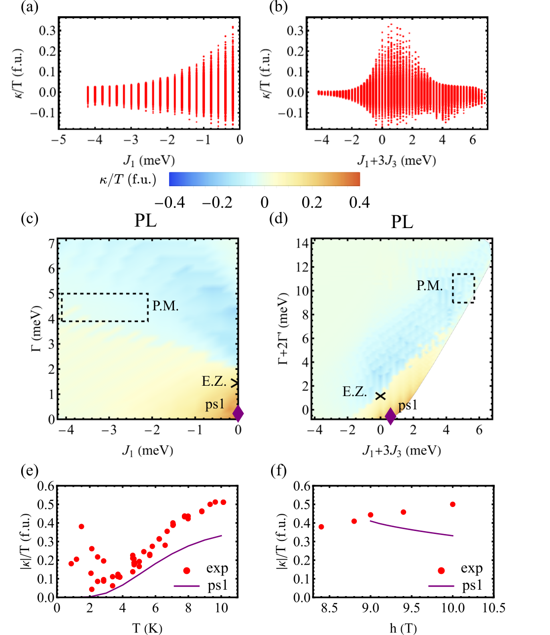
An alternative way of looking at the data is to plot the maximum value of $\kappa^{2D}_{xy}/T$ as a false color on a two-dimensional plot with axes given by $J_{1}$ and $\Gamma$, which we do in Fig. 2(c), or following the strategy proposed in Ref. Maksimov and Chernyshev 2020, with the axes formed by effective couplings $\tilde{J}=J_{1}+3J_{3}$ and $\tilde{\Gamma}=\Gamma+2\Gamma^{\prime}$, shown in Fig. 2(d). Each data point in these panels is taken to be the maximal value of $|\kappa^{2D}_{xy}|/T$ from varying the remaining parameters. We find that the largest $|\kappa^{2D}_{xy}|/T$ in the PL phase (at $h=10$ T and $T=10$ K) never exceeds about 0.35 f.u. in the fermionic units. To orient the reader, we show with the dashed rectangle what the authors of Ref. Maksimov and Chernyshev 2020 call the “realistic parameter regime,” and the cross represents the parameter set chosen in Ref. Zhang et al. 2021. In both regions, we find $|\kappa^{2D}_{xy}|/T$ to be less than 0.2 f.u., far from 0.5 f.u. reported in Ref. Kasahara et al. 2018 and much below the maximum value measured in Ref. Czajka et al. 2022.

Finally, we select the parameter set (labeled ps1) with the largest value of thermal Hall effect in our data and plot its value as a function of temperature and field, shown in Figs. 2(e,f). While the monotonically increasing temperature dependence observed in Ref. Czajka et al. 2022 is qualitatively reproduced, the field dependence is opposite – the experiment shows an increasing $|\kappa_{xy}(h)|$, while our data invariably decrease monotonically. Its physical reason is clear – in the fully polarized phase, the increase of the magnetic field leads to the (linear in field) growth of the magnon gap $\epsilon_{\text{min}}$. And since the Berry curvature integrand in Eq. (2) is weighted by the function $c_{2}(f(\epsilon))\propto\exp(-\epsilon/T)$, its value is exponentially suppressed at the experimentally relevant temperatures, leading to the decrease in $|\kappa_{xy}(h)|$. We thus conclude that not only is the magnon contribution too low to account for the experimental value of thermal Hall effect, but its field dependence in the fully polarized phase cannot reproduce the experiment neither.

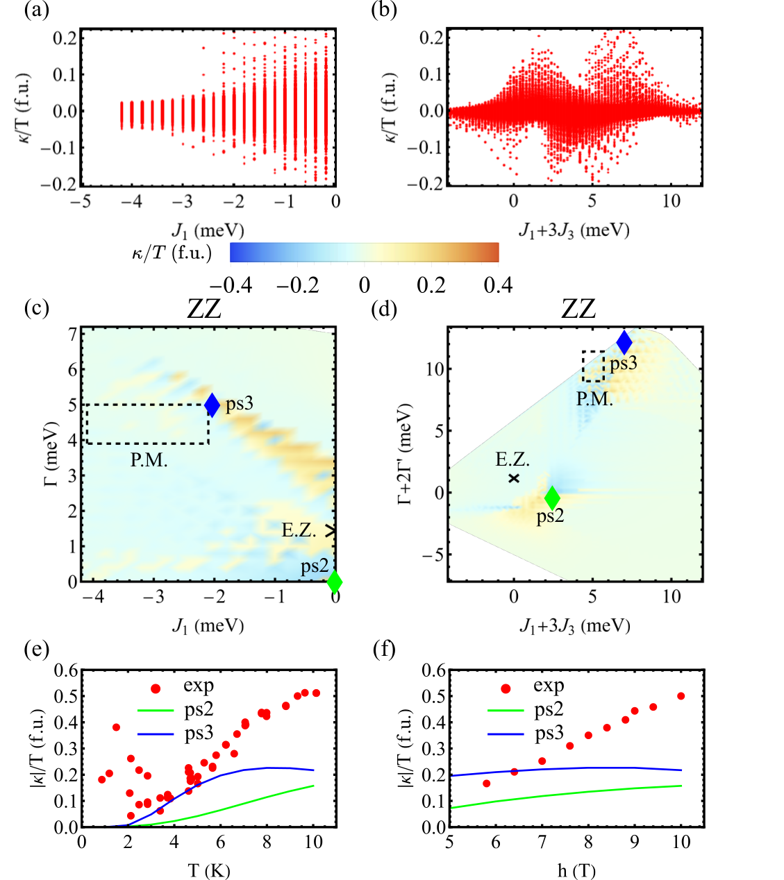
We therefore turn our attention to the zigzag phases, with the distributions of $\kappa_{xy}^{2D}/T$ along the $J_{1}$ and $\tilde{J}=J_{1}+3J_{3}$ shown in Figs. 3 (a) and (b), respectively, evaluated at $h=10$ T and $T=10$ K as before. Similarly to the PL phase, the magnitude of the Hall conductivity increases with the decreasing $|J_{1}|$. The maximum value of $\kappa^{2D}_{xy}/T$ is plotted as a false color map in $(J_{1},\Gamma)$ and $(\tilde{J},\tilde{\Gamma})$ coordinates, respectively, in Figs. 3(c) and (d). We find the largest value of $\kappa^{2D}_{xy}/T$ to be about 0.2 f.u. When considering the “realistic parameter regime” in Ref. Maksimov and Chernyshev 2020 (dashed region) or the parameters used in Ref. Zhang et al. 2021 (cross), $\kappa^{2D}_{xy}/T$ does not exceed 0.15 f.u., far below the experimentally reported values Kasahara et al. 2018; Yokoi et al. 2021; Czajka et al. 2022.

To compare with the experimental data, we choose two sets of parameters (labeled ps2 and ps3 in Fig. 3, the values are listed in the caption) that belong to the ZZ1 and ZZ2 phases, respectively, and which have the largest values of $|\kappa_{xy}^{2D}|/T$ in our studied range. We evaluate the temperature and field dependence of $|\kappa^{2D}_{xy}|/T$ at these parameter sets and plot them against the experimental data from Ref. Czajka et al. 2022 in Figs. 3(e,f). Under the experimentally relevant conditions $2<T<6$ K and $6<h<7$ T, we find that the parameter set ps2 qualitatively matches the trends in the temperature and field dependence of the experimental thermal Hall data. Near $T=10$ K and $h=10$ T, $\kappa_{xy}/T$ continues to increase for ps2 (as is the case experimentally); whereas for ps3 it starts to decline. However, as noted already and as seen from Figs. 3(e,f), the computed magnitude of $|\kappa^{2D}_{xy}|/T$ is well below the experimental values. This indicates that the intrinsic magnon contribution alone cannot fully account for the measured thermal Hall conductivity in $\text{$\alpha$}\text{-}\text{RuCl}{\vphantom{\text{X}}}_{\smash[t]{\text{3}}}$. We thus turn our attention to additional, bosonic in nature contributions to the thermal Hall effect.

Phonon contribution to the thermal Hall effect. We now turn to investigate other effects that may enhance the thermal Hall effect. Recent experimental data Lefrançois et al. 2022 on $\text{$\alpha$}\text{-}\text{RuCl}{\vphantom{\text{X}}}_{\smash[t]{\text{3}}}$  show that the temperature dependence of $\kappa_{xy}$ resembles closely that of longitudinal thermal conductivity $\kappa_{xx}$, as demonstrated in Fig. 4(a), with the ratio between the two roughly the same ($0.03-0.10$%) across different samples, from which the authors of Ref. Lefrançois et al. 2022 conclude that phonons must play a key role in the thermal Hall effect. In an insulator, the logitudinal $\kappa_{xx}$ is dominated by non-chiral acoustic phonons. The thermal Hall effect by contrast is time-reversal odd and chiral in nature. We distinguish two mechanisms of such chiral phonon response: the intrinsic one, due to the Berry curvature induced by magnon-phonon coupling, and the extrinsic one, due to phonon scattering off of defects.

Intrinsic phonon contribution to $\kappa_{xy}$. The distance dependence of the superexchange interactions between Ru³⁺ ions leads naturally to the magnetoelastic (ME) coupling of the generic form (see SM for further details):

where $\vec{u}_{i}$ is the displacement of the ion at site $i$ from its equilibrium position. Writing these displacements in terms of the phonon operators $u_{i}^{\gamma}\sim(a_{i\gamma}^{\dagger}+a_{i\gamma})$ (with polarization $\gamma$), this results in the hybridization between the magnons and the phonon branches Kittel 2004; Liu et al. 2021; Lebert et al. 2022, endowing the phonons with the Berry curvature that contributes to $\kappa_{xy}$ just as in Eq. (2). The magnitude of the additional phonon contribution $\kappa_{xy}^{\text{(I)}}$ is related to the strength of the ME coupling, whose existence is supported by the softening of the phonon branch at small $q$-vectors meansured in experiments Li et al. 2021. Choosing the ME coupling that qualitatively reproduces the phonon softening (see SM for details), the value of $\kappa_{xy}/T$ is plotted in Fig. 4(b) with the solid blue line using the parameter set ps2 in the ZZ1 phase. As this figure shows, the magnitude of the intrinsic $\kappa^{I}_{xy}/T$ is enhanced compared to the magnon-only value in the temperature regime of interest $T>3$ K – the same conclusion was reached in the recent study Ref. Li and Okamoto 2022. However, the magnitude $\kappa^{I}_{xy}/T$ ends up still being smaller than the experimentally measured Hall signal, prompting us to consider additional, phonon contributions.

Extrinsic phonon contribution to $\kappa_{xy}$. There are multiple sources of phonon contributions to the thermal Hall effect, in analogy to the phonon contribution to the electronic Hall effect ($\sigma_{xy}$) in metals Nagaosa et al. 2010. One candidate mechanism is the intrinsic skew-scattering, which originates from the Lorentz force on ions Flebus and MacDonald 2022. Another source is the extrinsic skew-scattering from phonons scattering off of magnetic impurities Chen et al. 2020; Flebus and MacDonald 2022. However, after comparing the experimental data Lefrançois et al. 2022 with characteristic features of these effects (see SM for detailed analysis), we came to the conclusion that they are negligible in $\text{$\alpha$}\text{-}\text{RuCl}{\vphantom{\text{X}}}_{\smash[t]{\text{3}}}$.

Instead, the very weak temperature dependence of the ratio $\kappa_{xy}/\kappa_{xx}$ (see Fig. 4a) and absence of strong sample variability in recent experiments Lefrançois et al. 2022 indicate that the dominant extrinsic contribution to $\kappa_{xy}$ is most likely from the so-called side-jump scattering of phonons off of defects Nagaosa et al. 2010, which we demonstrate in the SM using the formalism recently developed in Ref. Guo et al. 2022. Crucially, this effect scales with the phonon mean-free path $\ell$, just like the longitudinal thermal conductivity, consistent with the ratio of the two being sample independent.

Using the experimental data from Ref. Lefrançois et al. 2022 at high temperatures $T\gtrsim|K|/k_{B}\approx 80K$, above the magnon bandwidth where the effects of the Kitaev physics and associated Berry curvature are unimportant, we determine the Hall angle due to extrinsic scattering $\theta_{H}^{E}\equiv\kappa_{xy}^{E}/\kappa_{xx}=(0.6\pm 0.2)\times 10^{-3}$. By contrast, at low temperatures $T\sim 10-15$ K where the interpretation of the thermal Hall measurements on $\text{$\alpha$}\text{-}\text{RuCl}{\vphantom{\text{X}}}_{\smash[t]{\text{3}}}$ is disputed, both the intrinsic (due to the Berry curvature) and extrinsic contributions to $\kappa_{xy}$ must be taken into account. By comparing the data in this low-$T$ region with the value $\theta_{H}^{E}$ from above, we are able to determine the phenomenological ratio $\eta\equiv\kappa_{xy}^{E}/\kappa_{xy}^{I}$. We obtain (see SM for details) $\eta=1.2\pm 0.5$ with the uncertainty related to the spread of the experimental data among the different samples. Taking the intrinsic $\kappa_{xy}^{I}$ (solid line in Fig. 4(b)) and multiplying by $(1+\eta)$, we thus obtain the total $\kappa_{xy}=\kappa_{xy}^{I}+\kappa_{xy}^{E}$, marked by the shaded blue region in Fig. 4(b). The experimental data from Ong’s group Czajka et al. 2022 fall inside the yellow shaded region. This indicates that the thermal Hall effect from the bosonic model given our parameter choice can explain the experimental observation.

Furthermore, given the flexibility in the magnitude of the ME coupling, we show (see SM) that choosing the largest physically allowed coupling results in the intrinsic value of $\kappa_{xy}^{I}/T$ of the order of 0.35 f.u. (for ps2), and further including the extrinsic effects can yield values of thermal Hall effect even in excess of the experimentally measured values. We thus conclude that the magnon-phonon mechanism proposed in this work is more than sufficient to explain the experimental thermal Hall data in $\text{$\alpha$}\text{-}\text{RuCl}{\vphantom{\text{X}}}_{\smash[t]{\text{3}}}$  without overly fine-tuning the model parameters, i.e., in a finite region in the parameter space.

Discussion. Having scanned a broad range of physically motivated parameters of the $(K,J_{1},J_{3},\Gamma,\Gamma^{\prime})$ generalized Kitaev–Heisenberg model, we conclude that the intrinsic magnon contribution alone is insufficient to explain the large observed magnitude of the thermal Hall effect in $\text{$\alpha$}\text{-}\text{RuCl}{\vphantom{\text{X}}}_{\smash[t]{\text{3}}}$. We further found that in order to reconcile the observed magnetic field dependence of the thermal Hall effect, it is necessary to conclude that $\text{$\alpha$}\text{-}\text{RuCl}{\vphantom{\text{X}}}_{\smash[t]{\text{3}}}$remains in the canted zigzag phase (as opposed to field polarized) in fields up to $\sim 10$ T. This conclusion is supported by the recent study by Li and Okamoto Li and Okamoto 2022 who found that the spin-phonon coupling tends to stabilize the canted zigzag phase for higher applied fields, compared to the pure spin model which would otherwise become fully polarized. Taking into account the spin-phonon coupling endows phonons with the chirality, contributing an additional intrinsic term to $\kappa_{xy}^{I}$, which however still falls short of explaining the experimental data, necessitating the inclusion of an extrinsic source of Hall effect. With minimal assumptions as to its mechanism, we used the existing experimental data to quantitatively arrive at the measure $\kappa_{xy}^{E}/\kappa_{xy}^{I}$ yielding values between 1 and 2, meaning that the extrinsic phonon contribution to $\kappa_{xy}$ is comparable, or a little larger, than the intrinsic Berry curvature effect. Taking both into account, we are able to explain not only the large magnitude but also the detailed temperature dependence of $\kappa_{xy}$, which is bosonic in nature.

Acknowledgements. The authors thank P. Ong, I. Sodemann and S. Winter for fruitful discussions, and L. Taillefer for the critical reading of the manuscript. H.Y. and A.H.N. were supported by the National Science Foundation Division of Materials Research under the Award DMR-1917511. S.L. was supported by the Robert A. Welch Foundation grant No. C-1818.

Supplementary Materials for “Magnons, Phonons, and Thermal Hall Effect in Candidate Kitaev Magnet $\alpha$-RuCl₃"

References

- Plumb et al. (2014) K. W. Plumb, J. P. Clancy, L. J. Sandilands, V. V. Shankar, Y. F. Hu, K. S. Burch, H.-Y. Kee, and Y.-J. Kim, Phys. Rev. B 90, 041112 (2014).
- Kitaev (2006) A. Kitaev, Annals of Physics 321, 2 (2006).
- Cao et al. (2016) H. B. Cao, A. Banerjee, J.-Q. Yan, C. A. Bridges, M. D. Lumsden, D. G. Mandrus, D. A. Tennant, B. C. Chakoumakos, and S. E. Nagler, Phys. Rev. B 93, 134423 (2016).
- Kasahara et al. (2018) Y. Kasahara, T. Ohnishi, Y. Mizukami, O. Tanaka, S. Ma, K. Sugii, N. Kurita, H. Tanaka, J. Nasu, Y. Motome, T. Shibauchi, and Y. Matsuda, Nature 559, 227 (2018).
- Yokoi et al. (2021) T. Yokoi, S. Ma, Y. Kasahara, S. Kasahara, T. Shibauchi, N. Kurita, H. Tanaka, J. Nasu, Y. Motome, C. Hickey, S. Trebst, and Y. Matsuda, Science 373, 568 (2021).
- Nasu et al. (2017) J. Nasu, J. Yoshitake, and Y. Motome, Phys. Rev. Lett. 119, 127204 (2017).
- Czajka et al. (2022) P. Czajka, T. Gao, M. Hirschberger, P. Lampen-Kelley, A. Banerjee, N. Quirk, D. G. Mandrus, S. E. Nagler, and N. P. Ong, Nature Materials 22, 36 (2022).
- McClarty et al. (2018) P. A. McClarty, X.-Y. Dong, M. Gohlke, J. G. Rau, F. Pollmann, R. Moessner, and K. Penc, Phys. Rev. B 98, 060404 (2018).
- Cookmeyer and Moore (2018) T. Cookmeyer and J. E. Moore, Phys. Rev. B 98, 060412 (2018).
- Chern et al. (2021) L. E. Chern, E. Z. Zhang, and Y. B. Kim, Phys. Rev. Lett. 126, 147201 (2021).
- Zhang et al. (2021) E. Z. Zhang, L. E. Chern, and Y. B. Kim, Phys. Rev. B 103, 174402 (2021).
- Li and Okamoto (2022) S. Li and S. Okamoto, Phys. Rev. B 106, 024413 (2022).
- Bruin et al. (2022) J. A. N. Bruin, R. R. Claus, Y. Matsumoto, N. Kurita, H. Tanaka, and H. Takagi, Nature Physics 18, 401 (2022).
- Lefrançois et al. (2022) É. Lefrançois, G. Grissonnanche, J. Baglo, P. Lampen-Kelley, J.-Q. Yan, C. Balz, D. Mandrus, S. Nagler, S. Kim, Y.-J. Kim, et al., Physical Review X 12, 021025 (2022).
- Jackeli and Khaliullin (2009) G. Jackeli and G. Khaliullin, Phys. Rev. Lett. 102, 017205 (2009).
- Rau et al. (2014) J. G. Rau, E. K.-H. Lee, and H.-Y. Kee, Phys. Rev. Lett. 112, 077204 (2014).
- Kim et al. (2015) H.-S. Kim, V. S. V., A. Catuneanu, and H.-Y. Kee, Phys. Rev. B 91, 241110 (2015).
- Kim and Kee (2016) H.-S. Kim and H.-Y. Kee, Phys. Rev. B 93, 155143 (2016).
- Winter et al. (2016) S. M. Winter, Y. Li, H. O. Jeschke, and R. Valentí, Phys. Rev. B 93, 214431 (2016).
- Chaloupka and Khaliullin (2016) J. Chaloupka and G. Khaliullin, Phys. Rev. B 94, 064435 (2016).
- Yadav et al. (2016) R. Yadav, N. A. Bogdanov, V. M. Katukuri, S. Nishimoto, J. Van Den Brink, and L. Hozoi, Scientific reports 6, 1 (2016).
- Winter et al. (2017) S. M. Winter, A. A. Tsirlin, M. Daghofer, J. van den Brink, Y. Singh, P. Gegenwart, and R. Valentí, Journal of Physics: Condensed Matter 29, 493002 (2017).
- Hou et al. (2017) Y. S. Hou, H. J. Xiang, and X. G. Gong, Phys. Rev. B 96, 054410 (2017).
- Winter et al. (2018) S. M. Winter, K. Riedl, D. Kaib, R. Coldea, and R. Valentí, Phys. Rev. Lett. 120, 077203 (2018).
- Eichstaedt et al. (2019) C. Eichstaedt, Y. Zhang, P. Laurell, S. Okamoto, A. G. Eguiluz, and T. Berlijn, Phys. Rev. B 100, 075110 (2019).
- Laurell and Okamoto (2020) P. Laurell and S. Okamoto, npj Quantum Materials 5 (2020), 10.1038/s41535-019-0203-y.
- Maksimov and Chernyshev (2020) P. A. Maksimov and A. L. Chernyshev, Phys. Rev. Research 2, 033011 (2020).
- Janssen et al. (2017) L. Janssen, E. C. Andrade, and M. Vojta, Phys. Rev. B 96, 064430 (2017).
- Suzuki and Suga (2018) T. Suzuki and S.-i. Suga, Phys. Rev. B 97, 134424 (2018).
- Kubota et al. (2015) Y. Kubota, H. Tanaka, T. Ono, Y. Narumi, and K. Kindo, Phys. Rev. B 91, 094422 (2015).
- Sears et al. (2020) J. A. Sears, L. E. Chern, S. Kim, P. J. Bereciartua, S. Francoual, Y. B. Kim, and Y.-J. Kim, Nature Physics 16, 837 (2020).
- Katsura et al. (2010) H. Katsura, N. Nagaosa, and P. A. Lee, Phys. Rev. Lett. 104, 066403 (2010).
- Matsumoto and Murakami (2011a) R. Matsumoto and S. Murakami, Phys. Rev. Lett. 106, 197202 (2011a).
- Matsumoto and Murakami (2011b) R. Matsumoto and S. Murakami, Phys. Rev. B 84, 184406 (2011b).
- Shindou et al. (2013) R. Shindou, J.-i. Ohe, R. Matsumoto, S. Murakami, and E. Saitoh, Phys. Rev. B 87, 174402 (2013).
- Murakami and Okamoto (2016) S. Murakami and A. Okamoto, J. Phys. Soc. Jpn. 86, 011010 (2016).
- Fukui et al. (2005) T. Fukui, Y. Hatsugai, and H. Suzuki, Journal of the Physical Society of Japan 74, 1674 (2005).
- Park and Yang (2019) S. Park and B.-J. Yang, Physical Review B 99, 174435 (2019).
- Chern et al. (2020) L. E. Chern, R. Kaneko, H.-Y. Lee, and Y. B. Kim, Phys. Rev. Res. 2, 013014 (2020).
- Kittel (2004) C. Kittel, Introduction to Solid State Physics, 8th ed. (Wiley, 2004).
- Liu et al. (2021) S. Liu, A. Granados del Águila, D. Bhowmick, C. K. Gan, T. Thu Ha Do, M. A. Prosnikov, D. Sedmidubský, Z. Sofer, P. C. M. Christianen, P. Sengupta, and Q. Xiong, Phys. Rev. Lett. 127, 097401 (2021).
- Lebert et al. (2022) B. W. Lebert, S. Kim, D. A. Prishchenko, A. A. Tsirlin, A. H. Said, A. Alatas, and Y.-J. Kim, Phys. Rev. B 106, L041102 (2022).
- Li et al. (2021) H. Li, T. T. Zhang, A. Said, G. Fabbris, D. G. Mazzone, J. Q. Yan, D. Mandrus, G. B. Halász, S. Okamoto, S. Murakami, M. P. M. Dean, H. N. Lee, and H. Miao, Nature Communications 12 (2021), 10.1038/s41467-021-23826-1.
- Nagaosa et al. (2010) N. Nagaosa, J. Sinova, S. Onoda, A. H. MacDonald, and N. P. Ong, Rev. Mod. Phys. 82, 1539 (2010).
- Flebus and MacDonald (2022) B. Flebus and A. H. MacDonald, Phys. Rev. B 105, L220301 (2022).
- Chen et al. (2020) J.-Y. Chen, S. A. Kivelson, and X.-Q. Sun, Phys. Rev. Lett. 124, 167601 (2020).
- Guo et al. (2022) H. Guo, D. G. Joshi, and S. Sachdev, Proc. Natl. Acad. Sci. U.S.A. 119, e2215141119 (2022).
- Mandal (2021) I. Mandal, Acta Phys. Pol. A 140, 372 (2021).
- (49) S. M. Winter, Private communication.