Master’s Thesis in Computational Mathematics Infinite-Dimensional Port-Hamiltonian Systems with a Moving Interface

Alexander Kilian
matriculation number: 77856
supervised by:
Prof. Dr. Fabian Wirth Dr. Andrii Mironchenko
Chair of Dynamical Systems
University of Passau
Prof. Dr. Bernhard Maschke
Laboratoire d’Automatique et de Génie des Procédés
Claude Bernard University Lyon 1

(December 20, 2021)

Eidesstattliche Erklärung

Hiermit erkläre ich, Alexander Kilian (Matrikelnummer 77856), gegenüber der Fakultät für Informatik und Mathematik der Universität Passau, dass ich die Masterarbeit mit dem Thema Infinite-Dimensional Port-Hamiltonian Systems with a Moving Interface selbstständig angefertigt und keine anderen als die angegebenen Quellen und Hilfsmittel benutzt habe. Alle wörtlich und sinngemäß übernommenen Ausführungen wurden als solche gekennzeichnet. Weiterhin erkläre ich, dass ich diese Arbeit in gleicher oder ähnlicher Form nicht bereits einer anderen Prüfungsbehörde vorgelegt habe.

Passau, den 20.12.2021

Alexander Kilian

Summary

This thesis deals with the formulation and analysis of two systems of conservation laws defined on two complementary intervals and coupled by some moving interface as a single infinite-dimensional port-Hamiltonian system. This approach may be regarded as an extension of the well-established mathematical framework of boundary port-Hamiltonian systems, i.e., infinite-dimensional Hamiltonian systems interacting with its physical environment.

A vast variety of multi-physics systems can be modeled as a Hamiltonian system, a special type of ordinary and partial differential equations. Such systems have a Hamiltonian, which describes the internally stored energy of the system. By allowing such systems to be open, one usually refers to this class of systems as (boundary) port-Hamiltonian systems. For the analysis of infinite-dimensional port-Hamiltonian systems, one combines the energy-based approach by means of Hamiltonians with the poweful framework of strongly continuous semigroups applied in infinite-dimensional systems theory. This approach has led to fundamental well-posedness and stability results in the field of infinite-dimensional port-Hamiltonian systems. Furthermore, the power flow at the spatial boundary has been utilized to control port-Hamiltonian systems.

The great success of this system description motivates to extend the port-Hamiltonian formulation to systems of conservation laws that are coupled by some moving interface. In order to keep track of the power flow at the position of the interface, one has to introduce interface port variables. In this thesis, we provide a well-posed port-Hamiltonian model of two distinct systems of conservation laws defined on two complementary, 1-dimensional spatial domains that are coupled by a fixed interface, and illustrate this result by reference to two transmission lines coupled through a resistor. Furthermore, we discuss under which boundary and interface conditions this system is exponentially stable. Since the formulation in case of a moving interface is quite troubled, we present some results that may be regarded as a first step towards a well-posed model, and debate the main issues that have to be tackled in the future.

Zusammenfassung

Ziel der Masterarbeit ist es, zwei auf komplementären Intervallen definierte Systeme von Energieerhaltungssätzen, die durch eine mobile Schnittstelle gekoppelt werden, mathematisch als ein unendlich-dimensionales port-Hamiltonsches System zu modellieren und zu analysieren. Dieses Modell kann als eine Verallgemeinerung der port-Hamiltonschen Formulierung linearer unendlich-dimensionaler Systeme, die mit ihrer Umgebung interagieren, verstanden werden.

Zahlreiche physikalische Prozesse können mathematisch mit Hilfe sogenannter Hamiltonscher Systeme modelliert werden. Diese besitzen eine Hamilton-Funktion, die in vielen Anwendungen die Systemenergie beschreibt. Erlaubt man einen Energieaustausch mit der Umgebung des Systems, so spricht man von port-Hamiltonschen Systemen, die sowohl durch gewöhnliche als auch partielle Differentialgleichungen beschrieben werden können. Bei der Untersuchung unendlich-dimensionaler port-Hamiltonscher Systeme verbindet man den abstrakten, funktionalanalytischen Ansatz mittels der Halbgruppentheorie mit dem auf Hamilton-Funktionen basierten, physikalisch motivierten Ansatz. Mit dieser Methodik ließen sich elementare Wohlgestelltheits- und Stabilitätsresultate auf dem Gebiet unendlich-dimensionaler port-Hamiltonscher Systeme beweisen. Darüber hinaus eignet sich das port-Hamiltonsche Modell aufgrund des Energieaustauschs mit der Umgebung bestens zur energiebasierten Regelung solcher Systeme.

Aufgrund des beachtlichen Erfolgs dieser Systembeschreibung soll in dieser Arbeit der Versuch einer port-Hamiltonschen Formulierung zweier Systeme von Energieerhaltungssätzen, die durch eine mobile Schnittstelle gekoppelt sind, unternommen werden. Dazu werden Schnittstellen-Port-Variablen eingeführt, um den Energiefluss an der sich bewegenden Schnitt- stelle zu modellieren. Wir werden ein wohlgestelltes System des eben beschriebenen Szenarios im Falle einer fixen Schnittstellenposition präsentieren und dieses Resultat anhand zweier Übertragungsleitungen mit unterschiedlichen physikalischen Eigenschaften, die durch einen elektrischen Widerstand gekoppelt werden, illustrieren. Ferner werden wir charakterisieren, unter welchen Rand- und Schnittstellenbedingungen ein solches System exponentiell stabil ist. Die port-Hamiltonsche Formulierung im Falle einer mobilen Schnittstellen ist problembeladen. Wir werden daher Probleme und offene Fragen, die es in Zukunft noch zu klären gilt, ausführlich diskutieren und für den Wohlgestelltheits-Nachweis essentielle Eigenschaften des modellierten Systems präsentieren.

Notation

Symbol	Description
$\mathbb{N}$ , $\mathbb{R}$ , $\mathbb{C}$	the set of natural, real, and complex numbers, respectively
$\mathbb{R}_{>0}$	the set of positive real numbers
$\mathbb{R}_{+}$	the set of non-negative real numbers
$\mathbb{F}^{m\times n}$	the vector space of $m\times n$ -matrices with entries in $\mathbb{F}$
$\mathbb{F}^{n}$	the vector space of $n$ -dimensional column vectors with entries in $\mathbb{F}$
$\realpart(z)$	real part of $z\in\mathbb{C}$
$\\|\cdot\\|_{2}$	Euclidean norm on $\mathbb{R}^{n}$
$\\|\cdot\\|_{\operatornorm\colon D(A)\to X}$	operator norm of an operator $A\colon D(A)\subset X\to X$
$\\|\cdot\\|_{\mathcal{L}(X)}$	operator norm on $\mathcal{L}(X)$
$X^{\prime}$	dual space of a vector space $X$
$\langle\cdot,\cdot\rangle_{X^{\prime}\times X}$	natural pairing between a vector space $X$ and its dual space $X^{\prime}$
$\langle\cdot\mid\cdot\rangle$	power pairing defined on a Hilbert space
$\ll\cdot,\cdot\gg$	plus pairing associated with a power pairing
$M^{\top}$ , $v^{\top}$	transpose of a matrix $M\in\mathbb{F}^{m\times n}$ /a vector $v\in\mathbb{F}^{n}$
$M>N$ $(M\geq N)$	positive (semi-)definiteness of $M-N\in\mathbb{F}^{n\times n}$
$A^{\ast}$	(formal) Hilbert space adjoint of an operator $A$
$S^{\bot}$	orthogonal complement of the space $S$
$S^{\perp\!\!\!\perp}$	orthogonal complement of $S$ with respect to the plus pairing
$L^{1}([a,b],\mathbb{F}^{n})$	vector space of $\mathbb{F}^{n}$ -valued integrable functions on $[a,b]$
$L^{2}([a,b],\mathbb{F}^{n})$	vector space of $\mathbb{F}^{n}$ -valued square integrable functions on $[a,b]$
$\\|\cdot\\|_{L^{2}}=\\|\cdot\\|_{L^{2}(a,b)}$	standard $L^{2}$ -norm on $L^{2}([a,b],\mathbb{F}^{n})$
$L_{loc}^{1}([0,\infty),X)$	vector space of $X$ -valued locally integrable functions on $[0,\infty)$
$H^{N}([a,b],\mathbb{F}^{n})$	Sobolev space of order $N\in\mathbb{N}$ on $[a,b]$
$H_{loc}^{1}([0,\infty),X)$	vector space of $X$ -valued locally $H^{1}$ -functions on $[0,\infty)$
$\mathcal{C}([a,b],X)$	vector space of continuous functions $f\colon[a,b]\to X$ with finite norm
	$\\|f\\|_{\infty}:=\sup\limits_{x\in[a,b]}\\|f(x)\\|_{X}$

$\mathcal{C}^{k}([a,b],X)$	vector space of $k$ -times continuously differentiable functions $f\colon[a,b]\to X$
$\mathcal{C}^{\infty}(\mathbb{R}^{n},\mathbb{R})$	vector space of infinitely differentiable functions
$\mathcal{D}(\Omega)$	vector space of infinitely differentiable functions with compact
	support on $\Omega$ (the set of test functions on $\Omega$ )
$\mathcal{D}^{\prime}(\Omega)$	vector space of distributions on $\Omega$
$\langle u,\varphi\rangle_{\mathcal{D}^{\prime}(\Omega)}$	action of $u\in\mathcal{D}^{\prime}(\Omega)$ on a test function $\varphi\in\mathcal{D}(\Omega)$
$\mathcal{L}(X,Y)$	space of linear bounded operators from $X$ to $Y$
$\mathcal{L}(X)$	space of linear bounded operators on $X$
$I_{X}$ ( $I$ )	identity of the vector space $X$
$A_{\|\Omega}$	restriction of $A$ to the set $\Omega\subset D(A)$
$\overline{D(A)}$	closure of $D(A)\subset X$ with respect to $\\|\cdot\\|_{X}$
$\frac{dx}{dz}$	derivative of $x$ with respect to $z$
$\dot{x}=\frac{dx}{dt}$	derivative of $x$ with respect to time $t$
$\ddot{x}=\frac{d^{2}x}{dt^{2}}$	second derivative of $x$ with respect to time $t$
$\frac{\partial w}{\partial x_{i}}=\partial_{x_{i}}w$	partial derivative of $w(x_{1},\ldots,x_{n})$ with respect to $x_{i}$ , $i=1,\ldots,n$
$\nabla H(x)$	gradient column vector of $H\colon\mathbb{R}^{n}\to\mathbb{R}$
$\frac{\delta}{\delta x}H=\delta_{x}H$	variational derivative of a functional $H\colon L^{2}([a,b],\mathbb{R}^{n})\to\mathbb{R}$
$T_{x}X$	tangent space of $X$ at $x\in X$
$T_{x}^{\prime}X$	cotangent space of $X$ at $x\in X$
$A^{J}$	set of mappings $J\to A$ , with $J$ an index set
$\rho(A)$ , $\sigma(A)$	resolvent set and spectrum of an operator $A\colon D(A)\subset X\to X$
$f(x_{0}^{+})=\lim\limits_{x\searrow x_{0}}f(x)$	right-hand limit of $f$ at $x_{0}$
$f(x_{0}^{-})=\lim\limits_{x\nearrow x_{0}}f(x)$	left-hand limit of $f$ at $x_{0}$
$\mathcal{O}(\epsilon)$	big O notation with respect to $\epsilon$
$A\hookrightarrow B$	embedding of $A\subset B$ into $B$

Chapter 1 Introduction

1 Background

The port-Hamiltonian systems theory [11, 17, 27] is a systematic framework for modeling systems comprising various physical domains, such as mechanical, electric, hydraulic, and thermal domains. This approach is realized by classifying every (ideal) system component subject to its main physical characteristics, and by taking energy to be medium of communication between the physical domains in multi-physics systems. The eponymous concepts used for this modeling framework are the system’s Hamiltonian (that is, its total energy) stemming from mechanics [2], and the port-based modeling approach [22], which is based on the power-conserving interconnection of various system components by means of ports. They consist of physical quantities whose product yields power (e.g., current and voltage in an electrical network, or force and velocity in a mechanical system). That way, the power flow between the system’s components can be expressed. The resulting network structure can be geometrically described by a power-conserving interconnection structure, called the Dirac structure, which has proved to be highly valuable in the field of port-based modeling and analysis [7, 28].

There are three main features of port-Hamiltonian systems worth highlighting. Firstly, the (power-conserving) interconnection of port-Hamiltonian systems is again a port-Hamiltonian system. This is a crucial property and emphasizes the network structure of this framework. Secondly, this framework allows the inclusion of energy-dissipating elements, which is why port-Hamiltonian models are broadly applicable. Lastly, the port-Hamiltonian framework is greatly suitable for control purposes. It allows to model the interaction of the system with its environment by means of external ports which are, in particular, accessible for controller action.

Based on the theory of infinite-dimensional Hamiltonian systems in [21], the port-Hamiltonian formulation has been extended to infinite-dimensional systems [29]. The interconnection structure is generalized to a Stokes-Dirac structure, where the power flow through the boundary of the spatial domain, that is, the interaction with the system’s environment, is encompassed. Just as in the finite-dimensional case, this is essential for the interconnection of several Hamiltonian systems, and it is a good starting point for the purpose of control, hence the name boundary port-Hamiltonian systems. For the analysis of infinite-dimensional port-Hamiltonian systems one usually considers abstract Cauchy problems of the form

	$\displaystyle\dot{x}(t)$	$\displaystyle=A_{\mathcal{Q}}x(t),\hskip 14.22636ptt>0,$
	$\displaystyle x(0)$	$\displaystyle=x_{0}\in X,$

with $A_{\mathcal{Q}}\colon D(A_{\mathcal{Q}})\subset X\to X$ a linear (usually unbounded) operator on some Hilbert space $X$ that is associated with the port-Hamiltonian system. This port-Hamiltonian operator stores information concerning the interdomain coupling of the modeled multi-physics system as well as the mechanical and physical properties of the system. More precisely, these operators are usually given by $A_{\mathcal{Q}}=\mathcal{J}(\mathcal{Q}\cdot)$ , with $\mathcal{J}$ a formally skew-symmetric matrix differential operator modeling the interdomain coupling, and $\mathcal{Q}$ a coercive and bounded multiplication operator representing the physical properties. To prove well-posedness and stability results, one applies the well-documented theory of strongly continuous semigroups [8, 12, 23]. The most important class of semigroups in the framework of infinite-dimensional port-Hamiltonian systems are contraction semigroups, which are closely related to energy dissipation. Typically, one incorporates dissipation phenomena into the domain of the operator $A_{\mathcal{Q}}$ by means of the port variables, and proves that this operator is the infinitesimal generator of a contraction semigroup. For control purposes, it seems natural to let the controls and observations act at the boundary of the spatial domain, leading to the notion of (port-Hamiltonian) boundary control systems [13], [25, Chapter 10]. These systems have been extensively studied in the PhD theses [4, 31].

Due to the great success of this system description, quite recently it was investigated whether the port-Hamiltonian formulation of infinite-dimensional systems can be extended to first-order systems that are coupled by some moving interface [10]. There are several instances where a system’s spatial domain might be subdivided into areas where the intrinsic physical properties or even the aggregate phase differ. For example, one may consider two distinct gases separated by a moving piston, or liquid-solid phase transitions. The mathematical model of the latter is known as the Stefan problem [16]. A port-Hamiltonian formulation of the two-phase Stefan problem has already been tested in [32]. In contrast to boundary port-Hamiltonian systems, this formulation yields an abstract port-Hamiltonian control system with the input being the velocity of the interface, and offers a new field of research in terms of interface control.

In this thesis, we review the port-Hamiltonian formulation of two systems of conservation laws defined on two complementary intervals that are coupled by a moving interface, as elaborated in [10], and further examine this class of systems. Our final objective is to collect some useful results concerning the underlying port-Hamiltonian operators by means of the theory of strongly continuous semigroups that may help to prove well-posedness and stability results with respect to the position of the moving interface. The main contributions made in this thesis are the following:

$\bullet$

We specify the Stokes-Dirac structure of the model proposed in [10] with respect to a formally skew-symmetric matrix differential operator in case of a fixed interface, see Proposition 17.5.
$\bullet$

If we allow for dissipation at the boundary and at the interface position, then the port-Hamiltonian operator associated with two systems of conservation laws that are coupled by a fixed interface is the infinitesimal generator of a contraction semigroup on the respective energy space. In particular, the underlying model is well-defined, see Theorem 19.9.
$\bullet$

Under some more restrictive assumption concerning the boundary condition, the generated semigroup is exponentially stable, see Theorem 19.16.
$\bullet$

We consider a simplified model which is closely related to the one formulated in [10], and present criteria for the stability of the associated family of port-Hamiltonian operators that encompasses the position of the moving interface, see Subsection 19.6.

2 Outline of this Thesis

The remaining chapters are organized as follows:

Chapter 2 aims to present the basic concepts and notions of port-based modeling. We deal with the port-Hamiltonian formulation of finite-dimensional multi-physics systems, where we restrict ourselves to linear systems. To that end, we introduce the fundamental concept of a power-conserving interconnection structure, called a Dirac structure, and briefly discuss its constituting port variables. This allows us to define the port-Hamiltonian dynamics by means of the underlying Dirac structure.

Chapter 3 covers some well-known notions and results from the literature that are used in the upcoming chapters. We will mainly recall the basics of infinite-dimensional systems theory and, with that said, we will recall the concept of strongly continuous semigroups and some important results that characterize their infinitesimal generators. Furthermore, we will discuss formally adjoint operators of matrix differential operators.

In Chapter 4 we generalize the port-Hamiltonian approach of Chapter 2 to infinite-dimen- sional systems, where we restrict ourselves to idealized systems with a 1-dimensional spatial domain. We discuss the main differences to finite-dimensional port-Hamiltonian systems, and show how the power flow at the boundary of the spatial domain is incorporated into the definition of the Dirac structure, leading to the notion of a boundary port-Hamiltonian system. This chapter sets a basis for the discussion in the following chapter.

Chapter 5 is the centerpiece of this thesis and studies the port-Hamiltonian formulation of a system of two conservation laws with a moving interface. The main goal is to provide a well-posed model for a system of two conservation laws on two complementary intervals separated by an interface, where we take the interface’s velocity to be the input variable of the system. It turns out that this formulation poses delicate problems. Therefore, we vastly simplify the original problem, and work out some important properties of the simplified system that may help to further investigate the initial one.

In Chapter 6 we summarize the covered topics and reflect the main contributions made in this work. Furthermore, we draw our conclusions from the discussion in Chapter 5 and give some comments on open problems and potential future work concerning this rather new class of systems.

Chapter 2 Finite-Dimensional Port-Hamiltonian Systems

In this chapter, we want to study basic concepts of port-based network modeling and provide the definition of finite-dimensional port-Hamiltonian systems and their underlying Dirac structures. Section 3 is devoted to the description of the main characteristics of port-based network modeling, which originates in the work of Paynter [22]. To this end, we consider the model of a simple mass-spring system. This motivates to introduce the port-Hamiltonian formulation of multi-physics systems. The dynamics of port-Hamiltonian systems are geometrically specified by so-called Dirac structures. In Section 4 we will introduce this fundamental concept and give some examples of Dirac structures. In the Sections 5, 6, and 7 we briefly discuss energy-storing, energy-dissipating, and external ports, respectively. In the finite-dimensional case, these are the constitutive ports of a Dirac structure. After that, we are finally able to geometrically define the dynamics of port-Hamiltonian systems, which we are going to do in Section 8. As mentioned in the beginning, the port-Hamiltonian framework is particularly convenient for control purposes. Therefore, we will provide a state-space representation of a huge class of port-Hamiltonian systems that is suitable to be taken as the starting point for investigating control theoretical aspects. We will mainly focus on linear port-Hamiltonian systems.

The whole chapter relies heavily on the Chapters 2, 3, and 4 in [27], and on [11, Section 2.2].

3 A Motivating Example

In order to motivate the framework of port-based modeling, we start with a simple example.

Example 2.1 (Mass-Spring System; Example 2.1 in [27])

Consider a point mass with mass $m\in\mathbb{R}_{>0}$ , moving in one direction and without friction under the influence of a spring force corresponding to a linear spring with spring constant $k\in\mathbb{R}_{>0}$ . The usual way of modeling this mass-spring system is by means of the second-order differential equation

\displaystyle m\ddot{z}(t)=-k(z(t)-z_{0}),

(1)

where $z(t)\in\mathbb{R}$ denotes the position of the mass at time instant $t\geq 0$ , and $z_{0}\in\mathbb{R}_{>0}$ is the length of the spring at rest. In order to present the basic principles of port-based network modeling, we consider this problem from a different perspective. The mass-spring system is now regarded as the interconnection of two subsystems storing energy, namely the spring system storing potential energy and the mass system storing kinetic energy, see Figure 1.

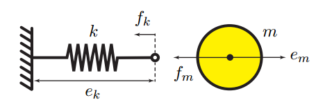
Refer to caption — Figure 1: Mass-Spring System Regarded as the Interconnection of two Subsystems [27, Figure 2.1]

For the spring system the potential energy is expressed in terms of the elongation $q=z-z_{0}$ of the spring. Assuming a linear spring, according to Hooke’s law the potential energy is given as $E_{\text{pot}}(q)=\frac{1}{2}kq^{2}$ . This leads to the spring system equations

\displaystyle\text{spring system}\colon\begin{cases}\dot{q}=-f_{k},\\ e_{k}=\frac{d}{dq}E_{\text{pot}}(q),\end{cases}

where $-f_{k}$ denotes the velocity of the endpoint of the spring where it is attached to the mass, and $e_{k}=kq$ describes the spring force at this endpoint.
For the mass system we obtain similar equations. Denoting the momentum of the mass by $p\in\mathbb{R}$ , the kinetic energy is given as $E_{\text{kin}}(p)=\frac{1}{2m}p^{2}$ , which leads to the following mass system equations:

\displaystyle\text{mass system}\colon\begin{cases}\dot{p}=-f_{m},\\ e_{m}=\frac{d}{dp}E_{\text{kin}}(p).\end{cases}

Here, $-f_{m}$ denotes the force exerted on the mass, and $e_{m}=\frac{p}{m}$ is the velocity of the mass.
These separately regarded subsystems are now interconnected through Newton’s third law in the following way:

	$\displaystyle-f_{k}$	$\displaystyle=e_{m},$
	$\displaystyle f_{m}$	$\displaystyle=e_{k}.$

The system’s stored energy is given by the Hamiltonian $H\colon\mathbb{R}^{2}\to\mathbb{R}$ defined by

\displaystyle H(q,p)=E_{\text{pot}}(q)+E_{\text{kin}}(p)=\frac{1}{2}kq^{2}+\frac{1}{2m}p^{2}.

(2)

The interconnected system can be written in terms of the Hamiltonian as follows:

\displaystyle\begin{bmatrix}\dot{q}\\ \dot{p}\end{bmatrix}=\begin{bmatrix}0&1\\ -1&0\end{bmatrix}\begin{bmatrix}\frac{\partial H}{\partial q}(q,p)\\ \frac{\partial H}{\partial p}(q,p)\end{bmatrix}.

(3)

These are the so-called Hamiltonian equations for the mass-spring system. Note that (3) is equivalent to the second-order model (1) by the correspondence $q=z-z_{0}$ : we have

\displaystyle m\ddot{z}=m\ddot{q}=m\dot{\left(\frac{\partial H}{\partial p}(q,p)\right)}=m\dot{\frac{p}{m}}=-\frac{\partial H}{\partial q}(q,p)=-kq=-k(z-z_{0}).

$\Diamond$

Remark 2.2

The reason for the minus sign in front of $f_{k}$ in Example 2.1 is that we want the product $f_{k}e_{k}$ between the spring’s velocity and force to be the incoming power with respect to the interconnection. The same applies for the product $f_{m}e_{m}$ between the exerted force on the mass and its velocity. This sign convention will be adopted throughout this chapter.

Despite its simplicity, Example 2.1 already displays some of the main characteristics of port-based network modeling: we regard the system as the coupling of the energy-storing spring system with the energy-storing mass system through a power-conserving interconnection where the power is routed from the mass system to the spring system and vice versa. This approach can be applied to general multi-physics systems, i.e., systems comprising different physical domains.

More generally, in port-based modeling a physical system is considered as the interconnection of three different types of ideal components:

(i)

Energy-storing elements: typical examples of energy-storing elements are ideal inductors (by means of the magnetic field), capacitors (by means of the electric field), masses, and springs.
(ii)

Energy-dissipating (or resistive) elements: examples of elements corresponding to energy-dissipation (due to friction, resistance, etc.) are resistors and dampers.
(iii)

Energy-routing elements: elements such as gyrators and transformers only redirect the power flow in the overall system [22, Part XV].

For the port-Hamiltonian formulation the energy-storing elements will be grouped into a single object denoted by $\mathcal{S}$ (’storage’), and correspondingly the energy-dissipating elements are grouped into a single object denoted by $\mathcal{R}$ (’resistive’). Moreover, the interconnection of all energy-routing elements can be considered as one energy-routing structure denoted by $\mathcal{D}$ , which we will call the system’s underlying Dirac structure.

The principle of port-Hamiltonian systems modeling is schematically illustrated in Figure 2: the energy-storing elements $\mathcal{S}$ and the energy-dissipating elements $\mathcal{R}$ are linked to a central interconnection (energy-routing) structure $\mathcal{D}$ . This linking is realized via pairs $(f,e)$ of vectors of flow and effort variables of equal dimension. We call a pair $(f,e)$ of vectors of flow and effort variables a port, and the total set of variables $f,e$ is called the set of port variables. The physical meaning of efforts and flows in various physical domains is listed in Table 1.

Physical Domain	Flow $f\in\mathcal{F}$	Effort $e\in\mathcal{E}$
electric	current $I$	voltage $V$
magnetic	voltage $V$	current $I$
potential translation	velocity $v$	force $F$
kinetic translation	force $F$	velocity $v$
potential rotation	angular velocity $\omega$	torque $T$
kinetic rotation	torque $T$	angular velocity $\omega$
potential hydraulic	volume flow $\phi$	pressure $p$
kinetic hydraulic	pressure $p$	volume flow $\phi$
chemical	chemical potential $\mu$	molar flow $f_{N}$
thermal	temperature $T$	entropy flow $f_{S}$

Table 1: Flows and Efforts Corresponding to their Physical Domains [11, Table 1.2]

Figure 2 shows three ports: the port $(f_{S},e_{S})$ linking to energy-storage, the port $(f_{R},e_{R})$ corresponding to energy-dissipation, and the external port $(f_{P},e_{P})$ , by which the system interacts with its environment.

In the following sections, we will provide more details about the fundamental notion of a Dirac structure on finite-dimensional spaces. To this end, we discuss the constituting ports of Dirac structures in the finite-dimensional case. We will treat successively energy-storing elements, energy-dissipating (resistive) elements, and external ports. After a short comment on state choice of different physical domains, we finally get to the basic geometric definition of a port-Hamiltonian system. Subsequently, we will present some simple yet important examples of such systems.

4 Dirac Structures

The key property of a Dirac structure is power conservation, meaning that it links the port variables in such a way that the total power entering or leaving a Dirac structure always amounts to zero. For the definition of a Dirac structure, we need to define the spaces of flows and efforts as well as the power flow defined on these spaces. We denote by $\mathcal{F}$ some finite-dimensional linear space of flows. Its elements will be denoted by $f\in\mathcal{F}$ , and are called flow (or energy) variables. The space of effort (or co-energy) variables is given by the dual linear space $\mathcal{E}=\mathcal{F}^{\prime}$ , and its elements are denoted by $e\in\mathcal{E}$ . The total space of flow and effort variables is $\mathcal{B}=\mathcal{F}\times\mathcal{E}$ , and is called the space of port variables or the bond space. The power on the total space of port variables is defined by

\displaystyle P\colon\mathcal{B}\to\mathbb{R},\hskip 14.22636pt(f,e)\mapsto\langle e\mid f\rangle,

(4)

where $\langle\cdot\mid\cdot\rangle\colon\mathcal{E}\times\mathcal{F}\to\mathbb{R}$ is the so-called power pairing. In the finite-dimensional case the power pairing $\langle\cdot\mid\cdot\rangle$ equals the natural pairing $\langle\cdot,\cdot\rangle_{\mathcal{F}^{\prime}\times\mathcal{F}}$ on the respective vector space, see Section 9. Usually, one may take $\mathcal{F}=\mathbb{R}^{k}$ and thus $\mathcal{E}=\mathbb{R}^{k}$ , and the power pairing equals the standard inner product:

\displaystyle\langle e\mid f\rangle=\langle e,f\rangle_{2},\hskip 14.22636pt(f,e)\in\mathcal{B}.

With the data provided in Table 1 one may check that the (inner) product of flow and effort variables indeed equals power. However, we note that there are interesting cases where it is beneficial not to take $\mathcal{F}=\mathbb{R}^{k}$ . For instance, in three-dimensional mechanical systems one usually works with Lie algebras of different matrix groups (see [21, Section 1.4]). For further details we refer to [27, Chapter 3]. We will see in the Chapters 4 and 5 that in the infinite-dimensional case, the power pairing does, in general, not coincide with the natural pairing.

Now we are able to define the notion of a Dirac structure in the finite-dimensional case.

Definition 2.3 (Dirac Structure)

Consider a finite-dimensional linear space of flows $\mathcal{F}$ and its dual space of efforts $\mathcal{E}=\mathcal{F}^{\prime}$ . Let $P$ be the power mapping on the bond space $\mathcal{B}=\mathcal{F}\times\mathcal{E}$ given by (4). A linear subspace $\mathcal{D}\subset\mathcal{B}$ is called a (constant) Dirac structure if

(i)

$P_{|\mathcal{D}}\equiv 0$ , i.e., $P(f,e)=0$ for all $(f,e)\in\mathcal{D}$ , and
(ii)

$\dim(\mathcal{D})=\dim(\mathcal{F})$ .

Property (i) in Definition 2.3 corresponds to power conservation, and states the previously mentioned fact that the total power flow always equals zero. It can be shown that the maximal dimension of any subspace $\mathcal{D}\subset\mathcal{B}$ satisfying property (i) is equal to $\dim(\mathcal{F})$ . This claim follows immediately from an equivalent definition of a Dirac structure, which we will state next. Another advantage of this equivalent definition of a Dirac structure is that it can be generalized to the case of an infinite-dimensional vector space $\mathcal{F}$ , leading to the definition of an infinite-dimensional Dirac structure, as we will see in Chapter 4.

In order to give this equivalent characterization of a Dirac structure, we define a canonical bilinear form $\ll\cdot,\cdot\gg$ on the space $\mathcal{B}$ which is closely related to the power pairing:

\displaystyle\begin{split}\ll\cdot,\cdot\gg\colon\mathcal{B}\times\mathcal{B}&\to\mathbb{R},\\ ((f^{1},e^{1}),(f^{2},e^{2}))&\mapsto\hskip 2.84544pt\ll(f^{1},e^{1}),(f^{2},e^{2})\gg\hskip 2.84544pt:=\langle e^{1}\mid f^{2}\rangle+\langle e^{2}\mid f^{1}\rangle.\end{split}

(5)

This bilinear form is non-degenerate, that is, if $\ll(f^{1},e^{1}),(f^{2},e^{2})\gg=0$ for all $(f^{2},e^{2})\in\mathcal{B}$ , then necessarily $(f^{1},e^{1})=0$ . However, it is not positive definite. We call this bilinear form a plus pairing.

We will now show that the following equivalent definition of a Dirac structure indeed satisfies the properties stated in Definition 2.3.

Proposition 2.4 (Proposition 2.1 in [27])

\displaystyle\mathcal{D}=\mathcal{D}^{\perp\!\!\!\perp},

(6)

where $\mathcal{D}^{\perp\!\!\!\perp}$ denotes the orthogonal complement of $\mathcal{D}$ with respect to the plus pairing $\ll\cdot,\cdot\gg$ .

Proof 4.1.

” $\Rightarrow$ ”: Let $\mathcal{D}$ be a Dirac structure in the sense of Definition 2.3. Let $(f^{1},e^{1})$ , $(f^{2},e^{2})\in\mathcal{D}$ be arbitrary port variables. By linearity, we have $(f^{1}+f^{2},e^{1}+e^{2})\in\mathcal{D}$ . By virtue of property (i) in Definition 2.3, we conclude that

	$\displaystyle 0$	$\displaystyle=\langle e^{1}+e^{2}\mid f^{1}+f^{2}\rangle$
		$\displaystyle=\langle e^{1}\mid f^{1}\rangle+\langle e^{1}\mid f^{2}\rangle+\langle e^{2}\mid f^{1}\rangle+\langle e^{2}\mid f^{2}\rangle$
		$\displaystyle=\langle e^{1}\mid f^{2}\rangle+\langle e^{2}\mid f^{1}\rangle$
		$\displaystyle=\hskip 5.69046pt\ll(e^{1},f^{1}),(e^{2},f^{2})\gg,$

whence $\mathcal{D}\subset\mathcal{D}^{\perp\!\!\!\perp}$ . Moreover, as the plus pairing $\ll\cdot,\cdot\gg$ is non-degenerate, we have

\displaystyle\dim(\mathcal{D}^{\perp\!\!\!\perp})=\dim(\mathcal{F}\times\mathcal{E})-\dim(\mathcal{D})=2\dim(\mathcal{F})-\dim(\mathcal{D}),

and due to property (ii) in Definition 2.3, it follows that $\dim(\mathcal{D})=\dim(\mathcal{D}^{\perp\!\!\!\perp})$ and thus $\mathcal{D}=\mathcal{D}^{\perp\!\!\!\perp}$ .

” $\Leftarrow$ ”: Let $\mathcal{D}$ satisfy (6). Then for every $(f,e)\in\mathcal{D}$ we have in particular that

\displaystyle 0=\ll(f,e),(f,e)\gg=2\langle e\mid f\rangle=2P(f,e).

Thus, property (i) is satisfied. Again, as the plus pairing $\ll\cdot,\cdot\gg$ is non-degenerate, we obtain

\displaystyle\dim(\mathcal{D}^{\perp\!\!\!\perp})=2\dim(\mathcal{F})-\dim(\mathcal{D}).

(7)

Equation (6) now implies that $\dim(\mathcal{D})=\dim(\mathcal{F})$ , and hence property (ii) of a Dirac structure is satisfied as well.

In order to prove the alternative characterization, we first note that we have shown that property (i) implies $\mathcal{D}\subset\mathcal{D}^{\perp\!\!\!\perp}$ . Together with equation (7) this yields that any subspace $\mathcal{D}$ satisfying property (i) has the property that $\dim(\mathcal{D})\leq\dim(\mathcal{F})$ . In conclusion, a Dirac structure indeed is the linear subspace of maximal dimension satisfying property (i) of Definition 2.3.

There are several examples of constant Dirac structures. We will present only a few of them and refer to [27, Section 2.2] for more.

Example 4.2 (Dirac Structures; cf. Section 2.2 in [27]).

Let $\mathcal{F}=\mathbb{R}^{n}$ and $\mathcal{E}=\mathcal{F}^{\prime}=\mathbb{R}^{n}$ . Consider the following examples of Dirac structures:

Let $J\colon\mathcal{E}\to\mathcal{F},$ $e\mapsto f=Je$ , with $J\in\mathbb{R}^{n\times n}$ a skew-symmetric matrix, i.e., $J=-J^{\top}$ . Then one can readily show that

\displaystyle\mathcal{D}_{J}:=\gra(-J):=\left\{(f,e)\in\mathcal{F}\times\mathcal{E}\mid-f=Je\right\}

is a Dirac structure. According to Proposition 2.4, we need to show that $\mathcal{D}_{J}=\mathcal{D}_{J}^{\perp\!\!\!\perp}$ with respect to $\ll\cdot,\cdot\gg$ defined in (5). Due to skew-symmetry of $J$ , for $(f^{1},e^{1}),(f^{2},e^{2})\in\mathcal{D}_{J}$ we have

	$\displaystyle\ll(f^{1},e^{1}),(f^{2},e^{2})\gg$	$\displaystyle=\langle e^{1},f^{2}\rangle_{2}+\langle e^{2},f^{1}\rangle_{2}$
		$\displaystyle=\langle e^{2},-Je^{1}\rangle_{2}+\langle e^{1},-Je^{2}\rangle_{2}$
		$\displaystyle=\langle e^{1},Je^{2}\rangle_{2}-\langle e^{1},Je^{2}\rangle_{2}$
		$\displaystyle=0.$

We conclude that $\mathcal{D}_{J}\subset\mathcal{D}_{J}^{\perp\!\!\!\perp}$ . Conversely, let $(f,e)\in\mathcal{D}_{J}^{\perp\!\!\!\perp}$ , that is, for all $(f^{1},e^{1})\in\mathcal{D}_{J}$ ,

	$\displaystyle 0$	$\displaystyle=\ll(f^{1},e^{1}),(f,e)\gg$
		$\displaystyle=\langle e^{1},f\rangle_{2}+\langle e,f^{1}\rangle_{2}$
		$\displaystyle=\langle e^{1},f\rangle_{2}+\langle e,-Je^{1}\rangle_{2}$
		$\displaystyle=\langle e^{1},f\rangle_{2}+\langle e^{1},Je\rangle_{2}.$

Consequently, for this equation to hold for all $(f^{1},e^{1})\in\mathcal{D}_{J}$ , we need $f=-Je$ , whence $(f,e)\in\mathcal{D}_{J}$ and therefore $\mathcal{D}_{J}^{\perp\!\!\!\perp}\subset\mathcal{D}_{J}$ . Altogether, $\mathcal{D}_{J}=\mathcal{D}_{J}^{\perp\!\!\!\perp}$ , and $\mathcal{D}_{J}$ is a Dirac structure.

As we will see, graphs of skew-symmetric linear maps in the finite-dimensional case, and (formally) skew-symmetric matrix differential operators in the infinite-dimensional case play a substantial role in the port-Hamiltonian framework.

Let $\mathcal{K}\subset\mathcal{F}$ be any subspace. Define

\displaystyle\mathcal{K}^{\bot}:=\left\{e\in\mathcal{E}\mid\langle e\mid f\rangle=0\hskip 2.84544pt\text{for all }f\in\mathcal{K}\right\}.

Then $\mathcal{D}=\mathcal{K}\times\mathcal{K}^{\bot}$ is a so-called separable Dirac structure (cf. [27, Definition 2.2]), i.e., for all $(f^{1},e^{1}),(f^{2},e^{2})\in\mathcal{D}$ we have

\displaystyle\langle e^{1}\mid f^{2}\rangle=0.

One can show that any separable Dirac structure is of the form $\mathcal{K}\times\mathcal{K}^{\bot}$ for an appropriately chosen subspace $\mathcal{K}\subset\mathcal{F}$ , see [27, Proposition 2.2]. A typical example for a separable Dirac structure is given by transformers. A transformer is an element linking two scalar bonds with flow and effort variables $(f^{1},e^{1}),(f^{2},e^{2})\in\mathbb{R}^{2}$ by

	$\displaystyle f^{2}$	$\displaystyle=\alpha f^{1},$
	$\displaystyle e^{1}$	$\displaystyle=-\alpha e^{2},$

with $\alpha\in\mathbb{R}\setminus\{0\}$ the transformer ratio. More precisely, let $\mathcal{F}=\mathcal{E}=\mathbb{R}^{2}$ and set $\mathcal{K}_{\alpha}=\left\{(f,\alpha f)\in\mathcal{F}\mid f\in\mathbb{R}\right\}$ . It is clear that $\mathcal{K}_{\alpha}^{\bot}=\left\{(-\alpha e,e)\in\mathcal{E}\mid e\in\mathbb{R}\right\}$ , and that $\dim(\mathcal{K}_{\alpha}\times\mathcal{K}_{\alpha}^{\bot})=\dim(\mathcal{F})=2$ , which is why $\mathcal{D}_{\alpha}=\mathcal{K}_{\alpha}\times\mathcal{K}_{\alpha}^{\bot}$ is indeed a separable Dirac structure. This can be easily generalized to the multi-port case.

$\Diamond$

As illustrated in Figure 2, the Dirac structure describes how energy is exchanged among various components in a physical system. In the following, we want to specify the port variables that constitute a (finite-dimensional) Dirac structure. We will give an overview concerning port variables related to energy-storing and energy-dissipating system elements as well as external ports.

5 Energy-Storing Elements

The energy-storing multi-port element $\mathcal{S}$ unifies all energy-storing elements of the system. The port variables of the Dirac structure associated with $\mathcal{S}=\mathcal{F}_{S}\times\mathcal{E}_{S}$ will be denoted by $(f_{S},e_{S})\in\mathcal{S}$ . The total energy storage of the system is defined by a Hamiltonian function $H\colon X\to\mathbb{R}$ on the state space $X$ . We restrict ourselves to the case where the state space is given by $X=\mathbb{R}^{n}$ . In general, the state space is a smooth (finite-dimensional) manifold, see [27, Chapter 3], [30]. In Chapter 4 we will discuss the extension to the infinite-dimensional case.

Before providing more details about energy-storing multi-port elements, we want to clarify briefly how the state variables have to be chosen in various physical domains, as they are closely related to the flows and efforts. In the common classification of domains, many domains are characterized by two types of states, namely the generalized displacement $q\in X$ and the generalized momentum $p\in X^{\prime}$ . Depending on the physical domain, one obtains the generalized displacement $q$ by time-integration of the flow variable $f\in\mathcal{F}$ , whereas the generalized momentum $p$ refers to time-integration of the effort variable $e\in\mathcal{E}$ . Table 2 is an extension of Table 1 and gives a summary of the generalized states in the respective physical subdomain. For more background information concerning this topic, we recommend the introductory chapter in [11].

Physical Domain	Flow	Effort	Generalized Displacement	Generalized Momentum
	$f\in\mathcal{F}$	$e\in\mathcal{E}$	$q=\int f\,dt$	$p=\int e\,dt$
electric	current $I$	voltage $V$	charge $Q$	magnetic flux linkage $\lambda$
magnetic	voltage $V$	current $I$	magnetic flux linkage $\lambda$	charge $Q$
potential translation	velocity $v$	force $F$	displacement $x$	momentum $p$
kinetic translation	force $F$	velocity $v$	momentum $p$	displacement $x$
potential rotation	angular velocity $\omega$	torque $T$	angular displacement $\theta$	angular momentum $b$
kinetic rotation	torque $T$	angular velocity $\omega$	angular momentum $b$	angular displacement $\theta$
potential hydraulic	volume flow $\phi$	pressure $p$	volume $V$	momentum of a flow tube $\Gamma$
kinetic hydraulic	pressure $p$	volume flow $\phi$	momentum of a flow tube $\Gamma$	volume $V$
chemical	chemical potential $\mu$	molar flow $f_{N}$	number of moles $N$	$-$
thermal	temperature $T$	entropy flow $f_{S}$	entropy $S$	$-$

Table 2: Flows, Efforts, and Generalized State Variables in Different Physical Domains
[11, Table 1.1]

The vector of flow variables is given by the rate $\dot{x}$ of the state $x\in X$ . Thus, for any (time-dependent) state $x\in X$ the flow vector $\dot{x}$ will be an element of the linear space $\mathcal{F}_{S}=T_{x}X$ , the tangent space of $X$ at $x\in X$ . In the given case $X=\mathbb{R}^{n}$ , the tangent space $T_{x}X$ may be identified with $X$ .

Furthermore, the vector of effort variables of the energy-storing multi-port element is given by the gradient vector $\nabla H(x)\in\mathcal{E}_{S}=T_{x}^{\prime}X$ , the dual space of the tangent space $T_{x}X$ , which again may be identified with $X^{\prime}=\mathbb{R}^{n}$ . Note that we define $\nabla H(x)$ , $x\in X$ , to be a column vector instead of a row vector. This convention will be applied throughout this work.

Now, in case of a time-dependent state $x(t)\in X$ , $t\geq 0$ , we obtain the following power-balance for the energy-storing multi-port element:

\displaystyle\frac{d}{dt}H(x(t))=\nabla H^{\top}(x(t))\dot{x}(t).

(8)

In the present case, the bond space is given by $\mathcal{B}=\mathcal{S}=\mathcal{F}_{S}\times\mathcal{E}_{S}$ , and the power-pairing $\langle\cdot\mid\cdot\rangle\colon\mathcal{E}_{S}\times\mathcal{F}_{S}\to\mathbb{R}$ is given by $\langle\cdot,\cdot\rangle_{2}$ . The interconnection of the energy-storing elements to the storage port $(f_{S},e_{S})\in X\times X^{\prime}$ of some Dirac structure $\mathcal{D}\subset X\times X^{\prime}$ is done by setting

\displaystyle f_{S}=-\dot{x}\hskip 8.5359pt\text{and}\hskip 8.5359pte_{S}=\nabla H(x).

(9)

Note that the minus sign in (9) has been placed in order to have a consistent power flow convention: $\nabla H^{\top}(x)\dot{x}$ is the power flowing into the energy-storing elements, whereas $e_{S}^{\top}f_{S}$ is the power flowing into the Dirac structure. Hence, with (4) and (9) the power-balance (8) can also be written as

\displaystyle\frac{d}{dt}H(x(t))=-e_{S}^{\top}(t)f_{S}(t)=-\langle e_{S}(t)\mid f_{S}(t)\rangle=0,\hskip 14.22636ptt\geq 0,

(10)

provided that $(f_{S}(t),e_{S}(t))\in\mathcal{D}$ for $t\geq 0$ . Equation (10) then expresses power conservation of the system.

6 Energy-Dissipating Elements

The second multi-port element $\mathcal{R}$ corresponds to internal energy dissipation, and its port variables are denoted by $(f_{R},e_{R})$ . These port variables are terminated on a static energy-dissipating (resistive) relation $\mathcal{R}$ . Let $\mathcal{F}_{R}=\mathbb{R}^{m}$ and $\mathcal{E}_{R}=\mathcal{F}_{R}^{\prime}=\mathbb{R}^{m}$ be the dual space of $\mathcal{F}_{R}$ . In general, a resistive relation $\mathcal{R}\subset\mathcal{F}_{R}\times\mathcal{E}_{R}$ is a set of the form

\displaystyle\mathcal{R}=\left\{(f_{R},e_{R})\in\mathcal{F}_{R}\times\mathcal{E}_{R}\mid R(f_{R},e_{R})=0,\hskip 2.84544pt\langle e_{R},f_{R}\rangle_{2}\leq 0\right\}.

(11)

We will call the subset $\mathcal{R}$ an energy-dissipating relation or a resistive structure. If we restrict ourselves to linear resistive structures, the mapping $R\colon\mathcal{F}_{R}\times\mathcal{E}_{R}\to\mathbb{R}$ will be of the form

\displaystyle R(f_{R},e_{R})=R_{f}f_{R}+R_{e}e_{R},

where $R_{f},R_{e}\in\mathbb{R}^{m\times m}$ . In order to guarantee that the second constitutive relation in (11) is satisfied whenever the first one is, we need to impose the following conditions on those matrices:

(i)

$R_{f}R_{e}^{\top}=R_{e}R_{f}^{\top}\geq 0$ and
(ii)

$\rank\left(\begin{bmatrix}R_{f}&R_{e}\end{bmatrix}\right)=\dim(\mathcal{F}_{R})=m$ .

If these conditions are satisfied, then we can equivalently rewrite the first constitutive condition in (11) as the requirement that there exists some vector $\lambda\in\mathbb{R}^{m}$ such that

\displaystyle f_{R}=R_{e}^{\top}\lambda\hskip 8.5359pt\text{and}\hskip 8.5359pte_{R}=-R_{f}^{\top}\lambda.

It is easy to check now that under these conditions we have $\langle e_{R},f_{R}\rangle_{2}\leq 0$ , and hence the second constitutive condition in (11) can be omitted. Altogether, a linear resistive structure is of the form

\displaystyle\mathcal{R}=\left\{(f_{R},e_{R})\in\mathcal{F}_{R}\times\mathcal{E}_{R}\mid R_{f}f_{R}+R_{e}e_{R}=0\right\}

(12)

with suitably defined matrices $R_{f},R_{e}\in\mathbb{R}^{m\times m}$ . For a system with energy-storing and resistive elements, the bond space is given by $\mathcal{B}=\mathcal{F}\times\mathcal{E}=(X\times\mathcal{F}_{R})\times(X^{\prime}\times\mathcal{E}_{R})$ , and the power pairing again equals the natural inner product. By definition, the Dirac structure $\mathcal{D}\subset\mathcal{B}$ of such a system satisfies the power-balance

\displaystyle\left\langle\begin{pmatrix}e_{S}\\ e_{R}\end{pmatrix}\,\Bigg|\,\begin{pmatrix}f_{S}\\ f_{R}\end{pmatrix}\right\rangle=e_{S}^{\top}f_{S}+e_{R}^{\top}f_{R}=0,\hskip 14.22636pt\left(\begin{pmatrix}f_{S}\\ f_{R}\end{pmatrix},\begin{pmatrix}e_{S}\\ e_{R}\end{pmatrix}\right)\in\mathcal{D}.

(13)

This leads, by substitution of (10) and (13), to

\displaystyle\frac{d}{dt}H(x(t))=-e_{S}^{\top}(t)f_{S}(t)=e_{R}^{\top}(t)f_{R}(t)\leq 0,\hskip 14.22636ptt\geq 0.

(14)

This inequality expresses the fact that the internally stored energy (the Hamiltonian) monotonically decreases in the presence of resistive elements.

An important special case of energy-dissipating relations occurs when the resistive relation can be expressed as

\displaystyle f_{R}=-F(e_{R}),

where $F\colon\mathbb{R}^{m}\to\mathbb{R}^{m}$ satisfies $e_{R}^{\top}F(e_{R})\geq 0$ for all $e_{R}\in\mathbb{R}^{m}$ . For linear resistive elements, we have $F(e_{R})=Re_{R}$ with $R\in\mathbb{R}^{m\times m}$ being symmetric and positive semi-definite. A typical example of a linear resistive structure is provided by a linear damper in a spring-mass-damper system, where $\mathcal{R}_{d}$ is given by

\displaystyle\mathcal{R}_{d}=\{(f_{R},e_{R})\in\mathbb{R}^{2}\mid f_{R}=-de_{R}\},

(15)

and where $d\in\mathbb{R}_{+}$ is the damping constant.

7 External Ports

The external port $(f_{P},e_{P})\in\mathcal{F}_{P}\times\mathcal{E}_{P}$ , where $\mathcal{F}_{P}=\mathbb{R}^{k}$ and $\mathcal{E}_{P}=\mathcal{F}_{P}^{\prime}$ , models the interaction of the system with its environment. This comprises different situations. For instance, there are port variables which are accessible for controller action (see [11, Chapter 5], [26, Chapter 7]), or there is an external port describing the interaction with the physical environment. Another important type of external port variables corresponds to source connections, as it is often the case in electrical circuits. For instance, in an electrical circuit with voltage source the system’s input is the voltage of the source, and the current through the source is set to be the resulting output variable. If one wishes to distinguish between these types of external ports, which in some cases may even be inevitable, one can divide the external port into a control port and an interaction port (cf. [11, Subsection 2.2.1]). However, we will not distinguish between them.

Now, taking the external port into account, for a Dirac structure

\displaystyle\mathcal{D}\subset X\times\mathcal{F}_{R}\times\mathcal{F}_{P}\times X^{\prime}\times\mathcal{E}_{R}\times\mathcal{E}_{P}

the power-balance (13) extends to

\displaystyle\left\langle\begin{pmatrix}e_{S}\\ e_{R}\\ e_{P}\end{pmatrix}\,\Bigg|\,\begin{pmatrix}f_{S}\\ f_{R}\\ f_{P}\end{pmatrix}\right\rangle=e_{S}^{\top}f_{S}+e_{R}^{\top}f_{R}+e_{P}^{\top}f_{P}=0,\hskip 14.22636pt\left(\begin{pmatrix}f_{S}\\ f_{R}\\ f_{P}\end{pmatrix},\begin{pmatrix}e_{S}\\ e_{R}\\ e_{P}\end{pmatrix}\right)\in\mathcal{D},

and (14) accordingly extends to

\displaystyle\frac{d}{dt}H(x(t))=-e_{S}^{\top}(t)f_{S}(t)=e_{R}^{\top}(t)f_{R}(t)+e_{P}^{\top}(t)f_{P}(t)\leq e_{P}^{\top}(t)f_{P}(t),\hskip 14.22636ptt\geq 0.

This inequality states that the increase of the internally stored energy is always less than or equal to the externally supplied power.

8 Port-Hamiltonian Dynamics

Now that we have discussed the constitutive ports of a Dirac structure and the corresponding power-balance, we want to present the underlying geometrical structure of port-Hamiltonian systems. We will begin with the definition of linear port-Hamiltonian systems by means of Dirac structures, and give a more familiar representation of a big class of such systems. At the end of this section, we will give some final remarks regarding non-linear port-Hamiltonian systems and port-Hamiltonian differential algebraic systems.

We begin with the definition of linear port-Hamiltonian systems with respect to an underlying Dirac structure.

Definition 8.1 (Linear Port-Hamiltonian System).

Consider the state space $X=\mathbb{R}^{n}$ and a Hamiltoninan $H\colon X\to\mathbb{R}$ defining energy storage. Furthermore, let $\mathcal{F}_{R}=\mathcal{E}_{R}=\mathbb{R}^{m}$ and $\mathcal{F}_{P}=\mathcal{E}_{P}=\mathbb{R}^{k}$ . A linear port-Hamiltonian system on $X$ is defined as a triple $(\mathcal{D},H,\mathcal{R})$ , consisting of a Dirac structure

\displaystyle\mathcal{D}\subset\mathcal{F}\times\mathcal{E}=(X\times\mathcal{F}_{R}\times\mathcal{F}_{P})\times(X^{\prime}\times\mathcal{E}_{R}\times\mathcal{E}_{P})

defined with respect to the power pairing $\langle\cdot\mid\cdot\rangle=\langle\cdot,\cdot\rangle_{2}\colon\mathcal{E}\times\mathcal{F}\to\mathbb{R}$ , with energy-storing ports $(f_{S},e_{S})\in X\times X^{\prime}$ , resistive ports $(f_{R},e_{R})\in\mathcal{F}_{R}\times\mathcal{E}_{R}$ , external ports $(f_{P},e_{P})\in\mathcal{F}_{p}\times\mathcal{E}_{P}$ , the Hamiltonian $H$ , and a linear resistive structure

\displaystyle\mathcal{R}\subset\mathcal{F}_{R}\times\mathcal{E}_{R}

of the form (12). Its dynamics are geometrically specified by the requirement that for all $t\geq 0$ we have

\displaystyle\left(\begin{pmatrix}-\dot{x}(t)\\ f_{R}(t)\\ f_{P}(t)\end{pmatrix},\begin{pmatrix}\nabla H(x(t))\\ e_{R}(t)\\ e_{P}(t)\end{pmatrix}\right)\in\mathcal{D}\hskip 8.5359pt\text{and}\hskip 8.5359pt(f_{R}(t),e_{R}(t))\in\mathcal{R}.

At the beginning of Chapter 2, we have already seen how a mass-spring system is modeled as a port-Hamiltonian system. We revisit this example to show that this is indeed a linear port-Hamiltonian system in the sense of Definition 8.1.

Example 8.2 (Mass-spring System Revisited).

Consider the mass-spring system from Example 2.1. The dynamics of this system are defined by equation (3). Defining the state space $X=\mathbb{R}^{2}$ with state vector $x=\begin{bmatrix}q\\ p\end{bmatrix}$ , and taking $\mathcal{F}_{S}=\mathcal{E}_{S}=X$ , one immediately sees that the underlying Dirac structure of this system is given by the graph of the skew-symmetric matrix $-J\in\mathbb{R}^{2\times 2}$ with

\displaystyle J=\begin{bmatrix}0&1\\ -1&0\end{bmatrix},\text{ i.e.,}\hskip 8.5359pt\mathcal{D}_{J}=\{(f_{S},e_{S})\in\mathcal{F}_{S}\times\mathcal{E}_{S}\mid-f_{S}=Je_{S}\}.

Here we have $-f_{S}=\begin{bmatrix}\dot{q}\\ \dot{p}\end{bmatrix}$ and $e_{S}=\begin{bmatrix}\frac{\partial H}{\partial q}\\ \frac{\partial H}{\partial p}\end{bmatrix}$ , where $H\colon X\to\mathbb{R}$ is the Hamiltonian given by (2). Note that the matrix $J$ is the one given on the right-hand side in (3). As there are neither external ports nor resistive elements, the dynamics of this linear port-Hamiltonian system is geometrically specified by

\displaystyle(f_{S}(t),e_{S}(t))=(-\dot{x}(t),\nabla H(x(t)))\in\mathcal{D},\hskip 14.22636ptt\geq 0.

Moreover, by skew-symmetry of $J$ , the power-balance as expected yields

\displaystyle\frac{d}{dt}H(q(t),p(t))=\left\langle\begin{pmatrix}kq(t)\\ \frac{p(t)}{m}\end{pmatrix}\Bigg|\begin{pmatrix}\dot{q}(t)\\ \dot{p}(t)\end{pmatrix}\right\rangle=-\langle e_{S}(t)\mid f_{S}(t)\rangle=0,\hskip 14.22636ptt\geq 0.

$\Diamond$

A state-space representation, as established for the mass-spring system in Example 2.1, is quite common. More general, an important class of linear port-Hamiltonian systems is obtained by considering Dirac structures which are the graph of a skew-symmetric map of the form

\displaystyle\begin{bmatrix}e_{S}\\ e_{R}\\ e_{P}\\ \end{bmatrix}\mapsto\begin{bmatrix}f_{S}\\ f_{R}\\ f_{P}\end{bmatrix}:=\begin{bmatrix}-J&-G_{R}&-G\\ G_{R}^{\top}&0&0\\ G^{\top}&0&0\end{bmatrix}\begin{bmatrix}e_{S}\\ e_{R}\\ e_{P}\\ \end{bmatrix},

with $J=-J^{\top}\in\mathbb{R}^{n\times n}$ , a linear dissipation relation $f_{R}=-\bar{R}e_{R}$ for some positive-semidefinite matrix $\bar{R}\in\mathbb{R}^{m\times m}$ , and $G_{R}\in\mathbb{R}^{n\times m}$ , $G\in\mathbb{R}^{n\times k}$ . This yields so-called input-state-output port-Hamiltonian systems of the form

\displaystyle\begin{split}\dot{x}&=\left[J-R\right]\nabla H(x)+Gu,\\ y&=G^{\top}\nabla H(x),\end{split}

(16)

with $R:=G_{R}\bar{R}G_{R}^{\top}\in\mathbb{R}^{n\times n}$ , and with $u=e_{P}$ the input vector and $y=f_{P}$ the output vector. This is a convenient representation for the investigation of control related problems for port-Hamiltonian systems, see [11, Chapter 5], [26, Chapter 7], [27, Chapter 15].

The following example aims to emphasize port-based network modeling of multi-physics systems. We also want to point to Example 2.5 in [27], where a port-Hamiltonian formulation for the dynamics of a DC motor is derived.

Example 8.3 (Levitated Ball System; Example 2.4 in [27]).

Consider the dynamics of an iron ball that is levitated by the magnetic field of a controlled inductor, as schematically depicted in Figure 3. The Hamiltonian $H\colon\mathbb{R}^{3}\to\mathbb{R}$ of this system - with $q\in\mathbb{R}$ the height of the ball, $m>0$ the ball’s mass, $p\in\mathbb{R}$ the vertical momentum, $\varphi\in\mathbb{R}$ the magnetic flux-linkage of the inductor, $R_{c}>0$ the coil’s resistance, $g>0$ the gravitational constant, $L(\cdot)$ the inductance depending on the height $q$ , $V\in\mathbb{R}$ the voltage across the inductor, and $I\in\mathbb{R}$ the current through the inductor - is defined as

\displaystyle H(q,p,\varphi)=E_{\text{pot}}(q)+E_{\text{kin}}(p)+E_{\text{mag}}(q,\varphi)=mgq+\frac{p^{2}}{2m}+\frac{\varphi^{2}}{2L(q)}.

The system dynamics are given by

\displaystyle\begin{split}\begin{bmatrix}\dot{q}\\ \dot{p}\\ \dot{\varphi}\end{bmatrix}&=\begin{bmatrix}0&1&0\\ -1&0&0\\ 0&0&-R_{c}\end{bmatrix}\begin{bmatrix}\frac{\partial H}{\partial q}\\ \frac{\partial H}{\partial p}\\ \frac{\partial H}{\partial\varphi}\end{bmatrix}+\begin{bmatrix}0\\ 0\\ 1\end{bmatrix}V,\\ I&=\frac{\partial H}{\partial\varphi}.\end{split}

(17)

Here, $e_{P}=V$ denotes the input and $f_{P}=I$ denotes the system’s output. Furthermore, the matrices $J$ , $R\in\mathbb{R}^{3\times 3}$ , and $G\in\mathbb{R}^{3}$ from (16) are given by

\displaystyle J=\begin{bmatrix}0&1&0\\ -1&0&0\\ 0&0&0\end{bmatrix},\hskip 8.5359ptR=\begin{bmatrix}0&0&0\\ 0&0&0\\ 0&0&R_{c}\end{bmatrix},\hskip 8.5359pt\text{and}\hskip 8.5359ptG=\begin{bmatrix}0\\ 0\\ 1\end{bmatrix}.

While the system description (17) may at first glance indicate that the mechanical and the magnetic part of the given system are decoupled, they are actually coupled, namely via the Hamiltonian $H$ : the magnetic energy $E_{\text{mag}}$ depends both on the flux $\varphi$ and the mechanical variable $q$ . Consequently, the evolution of the (mechanical) momentum variable $p$ depends on the magnetic variable $\varphi$ , and the evolution of the magnetic variable $\varphi$ depends on the mechanical variable $q$ . $\Diamond$

Needless to say, there exist nonlinear port-Hamiltonian systems as well. The major difference to linear port-Hamiltonian systems is that the state space $X$ becomes a smooth manifold, and the Dirac structure is not constant anymore, but is modulated by the state variables. Moreover, the spaces $\mathcal{F}_{S}$ and $\mathcal{E}_{S}$ become the tangent space and the cotangent space, respectively, as mentioned in Section 5. Furthermore, the input-state-output description (16) of nonlinear port-Hamiltonian systems becomes

\displaystyle\begin{split}\dot{x}&=[J(x)-R(x)]\nabla H(x)+G(x)u,\\ y&=G^{\top}(x)\nabla H(x).\end{split}

(18)

For details and some examples we refer to [26, Chapter 6], [27, Chapter 3], and the references specified therein.

When modeling dynamical systems, the appearance of algebraic equations next to differential equations is ubiquitous. For instance, in network modeling of physical systems, the interconnections between different dynamical components of the overall system almost unavoidably lead to algebraic constraints. Such systems are called linear port-Hamiltonian descriptor systems (port-Hamiltonian differential-algebraic systems), or short pHDAEs [6]. The geometric definition of port-Hamiltonian systems is quite handy, as it can even characterize the dynamics of pHDAEs by choosing the underlying Dirac structure suitably. This is the reason why in Definition 8.1 one usually refers to the triple $(\mathcal{D},H,\mathcal{R})$ as a (linear) port-Hamiltonian differential-algebraic system.

In this chapter, we have presented the basic concepts and main characteristics of the port-Hamiltonian framework on finite-dimensional spaces. We have learned that the centerpiece of this approach is the power-conserving interconnection structure $\mathcal{D}$ , called the Dirac structure. We have presented the basic definition of a Dirac structure and discussed its constituting ports in the finite-dimensional case, namely ports associated with energy-storing and energy-dissipating elements as well as external ports. Lastly, we have geometrically specified the dynamics of linear port-Hamiltonian systems by means of their underlying Dirac structures and have given a state-space representation for a huge class of port-Hamiltonian systems.

Now that we have gained a basic understanding of port-based modeling of physical systems, we want to study infinite-dimensional port-Hamiltonian systems in the upcoming chapters, to finally deal with the main topic of this thesis, namely the port-Hamiltonian formulation of a system of two conservation laws with a moving interface. In order to do so, we need to provide some background information concerning semigroup theory, infinite-dimensional systems theory, the concept of admissibility, and evolution equations. We will treat these subjects in the next chapter.

Chapter 3 Some Background on Functional Analysis and Systems Theory

In preparation for the main part of this thesis, we recall some well-known concepts and results on selected topics. Most of the time, we will give no proofs, but provide references regarding the respective topics. Furthermore, we will omit various topics that are usually covered in the literature, and only focus on aspects that are useful for the discussion in the following chapters.

This chapter is organized as follows. In Section 9 we recall the definition of the Hilbert space adjoint of a densely defined operator $A\colon D(A)\subset X\to X$ . Moreover, we introduce the notion of the formally adjoint operator of a matrix differential operator, and discuss the difference between the Hilbert space adjoint and the formal adjoint. As we will deal with infinite-dimensional (control) systems, we need a tool for the analysis of such systems. In Section 10 we are going to study strongly continuous semigroups and characterize their infinitesimal generators. In Section 11 we cover abstract (i.e. Hilbert space-valued) linear differential equations and give sufficient and necessary conditions for well-posedness of such systems. We will see that the framework of strongly continuous semigroups is a powerful tool for the analysis of so-called abstract Cauchy problems. Afterwards, we are going to shortly discuss infinite-dimensional control systems in Section 12. For a proper treatment of such systems, we need to introduce the extrapolation space $X_{-1}$ and the concept of admissible control operators. We will give criteria for when the mild solution of an abstract control system is a continuous $X$ -valued function. Section 13 is the last section of this chapter and deals with linear, time-variant evolution problems. We will study (two-parameter) evolution systems and define the notion of stability for a family of infinitesimal generators of $C_{0}$ -semigroups. We assume that the reader is acquainted with Riemann integrals of vector-valued functions [19, Section 3.1], the Lebesgue theory of vector-valued measurable functions, and Bochner intergrals [1, Section 1.1].

Unless stated otherwise, throughout this chapter we assume that $X$ is a real or complex separable Hilbert space with inner product $\langle\cdot,\cdot\rangle_{X}$ .

9 Adjoint and Formally Adjoint Operators

In this section, we want to define and highlight the difference of the Hilbert space adjoint of a matrix differential operator to its formal adjoint, and provide a simple example to illustrate this difference. For a detailed, more general discussion on formally adjoint operators we refer to [3, Chapter 13].

For the first part of this section, we follow [25, Section 2.9].

Definition 9.1.

Let $V$ and $Z$ be Hilbert spaces. An operator $J\in\mathcal{L}(V,Z)$ is called an isomorphism, or a unitary operator, from $V$ to $Z$ , if we have

\displaystyle\langle Jv,Jw\rangle_{Z}=\langle v,w\rangle_{V},\hskip 14.22636ptv,w\in V.

One may verify that $J\in\mathcal{L}(V,Z)$ is unitary if and only if $\|Jv\|_{Z}=\|v\|_{V}$ holds for all $v\in V$ , and $\ran(J)=Z$ .

For any Hilbert space $V$ , we denote by $\langle z,v\rangle_{V^{\prime}\times V}$ the functional $z\in V^{\prime}$ applied to $v\in V$ , so that $\langle\cdot,\cdot\rangle_{V^{\prime}\times V}$ is linear in the first component and antilinear in the second component. This pairing is called the natural (duality) pairing on $V$ . The norm on $V^{\prime}$ is defined as

\displaystyle\|z\|_{V^{\prime}}=\sup_{\stackrel{{\scriptstyle v\in V}}{{\|v\|_{V}=1}}}|\langle z,v\rangle_{V^{\prime}\times V}|,\hskip 14.22636ptz\in V^{\prime}.

There is an operator $J_{R}\colon V\to V^{\prime}$ satisfying

\displaystyle\langle J_{R}v,w\rangle_{V^{\prime}\times V}=\langle v,w\rangle_{V},\hskip 14.22636ptv,w\in V.

According to the Riesz representation theorem, $J_{R}$ is an isomorphism. We say that we identify the Hilbert space $V$ with its dual $V^{\prime}$ , if we do not distinguish between $v$ and $J_{R}v$ for all $v\in V$ .

In the following, we identify $X$ with its dual $X^{\prime}$ . Consider a linear and densely defined operator $A\colon D(A)\subset X\to X$ . We wish to associate a Hilbert space adjoint $A^{\ast}$ to $A$ . Its domain is given by

\displaystyle D(A^{\ast}):=\left\{y\in X\mid\langle A\cdot,y\rangle_{X}\colon D(A)\to\mathbb{R},\,x\mapsto\langle Ax,y\rangle_{X}\text{ is continuous}\right\}.

If $y\in D(A^{\ast})$ , then the Hahn-Banach theorem extends the functional

\displaystyle x\mapsto\langle Ax,y\rangle_{X}

to a continuous linear functional on $X$ . The Riesz representation theorem yields that there exists a unique element $z_{y}\in X$ such that this functional has the form

\displaystyle\langle\cdot,z_{y}\rangle_{X}.

For $y\in D(A^{\ast})$ we define $A^{\ast}y=z_{y}$ . Hence, it holds that

\displaystyle\langle Ax,y\rangle_{X}=\langle x,A^{\ast}y\rangle_{X},\hskip 14.22636ptx\in D(A),\,y\in D(A^{\ast}).

In other words, the domain of the Hilbert space adjoint $A^{\ast}$ of an operator $A$ is given by

\displaystyle D(A^{\ast})=\left\{y\in X\mid\exists!\,z_{y}\in X\colon\forall x\in D(A)\colon\langle Ax,y\rangle_{X}=\langle x,z_{y}\rangle_{X}\right\}.

(19)

The following definitions can be found in Section 3.2 and Section 3.7 in [25], and in [8, Appendix A.3.2].

Definition 9.2.

Let $A\colon D(A)\subset X\to X$ and $B\colon D(B)\subset X\to X$ be linear and densely defined.

(i)

$A$ is called symmetric, if

$\displaystyle\langle Ax,y\rangle_{X}=\langle x,Ay\rangle_{X},\hskip 14.22636ptx,y\in D(A).$
(ii)

$A$ is called skew-symmetric, if

$\displaystyle\langle Ax,y\rangle_{X}=-\langle x,Ay\rangle_{X},\hskip 14.22636ptx,y\in D(A).$
(iii)

If for all $x\in D(A)$ , $y\in D(B)$ it holds that

$\displaystyle\langle Ax,y\rangle_{X}=\langle x,By\rangle_{X},$

then $B\subset A^{\ast}$ , that is, $D(B)\subset D(A^{\ast})$ and $By=A^{\ast}y$ for all $y\in D(B)$ .
(iv)

$A$ is called self-adjoint if $A^{\ast}=A$ , that is, $D(A)=D(A^{\ast})$ and $Ax=A^{\ast}x$ for all $x\in D(A)$ .
(v)

$A$ is called skew-adjoint if $A^{\ast}=-A$ .
(vi)

$A$ is called coercive if it is self-adjoint and there exists some $m>0$ such that $A\geq mI_{X}$ , i.e.,

$\displaystyle\langle Ax,x\rangle_{X}\geq m\|x\|_{X}^{2},\hskip 14.22636ptx\in D(A).$

For the rest of this section, we restrict ourselves to matrix differential operators defined on a Sobolev space. For this type of operators, we want to introduce the notion of formally adjoint operators. Roughly speaking, the only difference to the Hilbert space adjoint is that the constitutive relations of its domain are relaxed in a way such that

\displaystyle\langle Ax,y\rangle_{X}=\langle x,A^{\ast}y\rangle_{X}\hskip 5.69046pt+\text{boundary terms},\hskip 14.22636ptx\in D(A),\,y\in D(A^{\ast}).

The discussion in Section 15 will clarify the necessity of allowing boundary terms concerning the relation between an operator and its formal adjoint.

Now, let $X=L^{2}([a,b],\mathbb{R}^{n})$ be endowed with the inner product

\displaystyle\langle x,y\rangle_{X}=\langle x,y\rangle_{L^{2}}=\int_{a}^{b}y^{\top}(z)x(z)\,dz,\hskip 14.22636ptx,y\in X.

Let us define the Sobolev spaces

	$\displaystyle H^{1}([a,b],\mathbb{R}^{n})$	$\displaystyle=\left\{x\in X\,\big\|\,x\text{ is absolutely continuous},\,\frac{dx}{dz}\in X\right\},$
	$\displaystyle H^{N}([a,b],\mathbb{R}^{n})$	$\displaystyle=\left\{x\in X\,\big\|\,x\text{ is absolutely continuous},\,\frac{dx}{dz}\in H^{N-1}([a,b],\mathbb{R}^{n})\right\},\hskip 14.22636ptN\geq 2,$

as well as

	$\displaystyle H_{0}^{1}([a,b],\mathbb{R}^{n})$	$\displaystyle=\left\{x\in H^{1}([a,b],\mathbb{R}^{n})\mid x(a)=x(b)=0\right\},$
	$\displaystyle H_{0}^{N}([a,b],\mathbb{R}^{n})$	$\displaystyle=\left\{x\in H^{N}([a,b],\mathbb{R}^{n})\cap H_{0}^{N-1}([a,b],\mathbb{R}^{n})\,\big\|\,\frac{dx}{dz}\in H_{0}^{N-1}([a,b],\mathbb{R}^{n})\right\},\hskip 14.22636ptN\geq 2.$

Furthermore, define the boundary trace operator $\trace\colon H^{N}\left([a,b],\mathbb{R}^{n}\right)\to\mathbb{R}^{2nN}$ by

\displaystyle\trace(x):=\begin{bmatrix}x(b)\\ \vdots\\ \frac{d^{N-1}x}{dz^{N-1}}(b)\\ x(a)\\ \vdots\\ \frac{d^{N-1}x}{dz^{N-1}}(a)\end{bmatrix},\hskip 14.22636ptx\in H^{N}\left([a,b],\mathbb{R}^{n}\right).

(20)

The boundary trace operator $\trace$ is linear, bounded, and surjective, see [3, Section 7.8]. It allows us to equivalently write for $N\in\mathbb{N}$ ,

\displaystyle H_{0}^{N}([a,b],\mathbb{R}^{n})=\left\{x\in H^{N}([a,b],\mathbb{R}^{n})\mid\trace(x)=0\right\}.

Now, consider the matrix differential operator $A\colon D(A)\subset X\to X$ given by

\displaystyle\begin{split}D(A)&=\left\{x\in X\mid x\in H^{N}([a,b],\mathbb{R}^{n}),\,W\trace(x)=0\right\},\\ Ax&=\sum_{i=0}^{N}P_{i}\frac{d^{i}x}{dz^{i}},\hskip 14.22636ptx\in D(A),\end{split}

(21)

with $P_{i}\in\mathbb{R}^{n\times n}$ , $i=0,\ldots,N$ , and $W\in\mathbb{R}^{n\times 2n}$ . In particular, we have $H_{0}^{N}([a,b],\mathbb{R}^{n})\subset D(A)$ .

Definition 9.3.

For the domain of the formal adjoint $A_{0}^{\ast}\colon D(A_{0}^{\ast})\subset X\to X$ of the matrix differential operator $A$ defined in (21) it holds that

\displaystyle D(A_{0}^{\ast})=\left\{y\in X\mid\langle A\cdot,y\rangle_{X}\colon H_{0}^{N}([a,b],\mathbb{R}^{n})\to\mathbb{R},\hskip 2.84544ptx\mapsto\langle Ax,y\rangle_{X}\text{ is continuous}\hskip 2.84544pt\right\}.

In other words, the formal adjoint of the differential operator $A$ defined in (21) is simply given by the adjoint of its restriction $A_{|H_{0}^{N}([a,b],\mathbb{R}^{n})}$ .

Next, we present the formal pendant of some of the notions introduced in Definition 9.2.

Definition 9.4.

Let $A\colon D(A)\subset X\to X$ be the matrix differential operator defined in (21).

(i)

$A$ is called formally symmetric, if

$\displaystyle\langle Ax,y\rangle_{X}=\langle x,Ay\rangle_{X},\hskip 14.22636ptx,y\in H_{0}^{N}([a,b],\mathbb{R}^{n}).$
(ii)

$A$ is called formally skew-symmetric, if

$\displaystyle\langle Ax,y\rangle_{X}=-\langle x,Ay\rangle_{X},\hskip 14.22636ptx,y\in H_{0}^{N}([a,b],\mathbb{R}^{n}).$

Let us clarify the difference by reference to some simple examples.

Example 9.5.

Consider the following examples.

(i)

[cf. Example 13.4 in [24]] Let $X=L^{2}([a,b],\mathbb{R})$ . Consider the operator $A\colon D(A)\subset X\to X$ given by

	$\displaystyle D(A)$	$\displaystyle=H^{1}([a,b],\mathbb{R}),$
	$\displaystyle Ax$	$\displaystyle=\frac{d}{dz}x,\hskip 14.22636ptx\in D(A).$

We claim that the Hilbert space adjoint and the formal adjoint of the operator $A$ are given by $A_{1}$ and $A_{2}$ , respectively, with

	$\displaystyle D(A_{1})$	$\displaystyle=H_{0}^{1}([a,b],\mathbb{R}),$
	$\displaystyle D(A_{2})$	$\displaystyle=D(A),$
	$\displaystyle A_{k}x$	$\displaystyle=-\frac{d}{dz}x,\hskip 14.22636ptx\in D(A_{k}),\,k=1,2.$

Note that for all $x\in D(A)$ , $y\in D(A_{1})$ we have

\displaystyle\langle Ax,y\rangle_{X}=\int_{a}^{b}\frac{d}{dz}x(z)y(z)\,dz=\big[x(z)y(z)\big]_{a}^{b}-\int_{a}^{b}x(z)\frac{d}{dz}y(z)\,dz=\langle x,A_{1}y\rangle_{X}.

Thus, $A_{1}\subset A^{\ast}$ . In particular, by virtue of the Cauchy-Schwarz inequality, for $y\in D(A_{1})$ we have

\displaystyle\sup_{\begin{subarray}{c}x\in D(A)\\ \|x\|_{X}=1\end{subarray}}|\langle Ax,y\rangle_{X}|\leq\sup_{\begin{subarray}{c}x\in D(A)\\ \|x\|_{X}=1\end{subarray}}\int_{a}^{b}|x(z)|\left|\frac{d}{dz}y(z)\right|\,dz\leq\sup_{\begin{subarray}{c}x\in D(A)\\ \|x\|_{X}=1\end{subarray}}\|x\|_{X}\left\|\frac{d}{dz}y\right\|_{X}\leq C_{y}.

Conversely, suppose that $y\in D(A^{\ast})\subset X$ . Set $\psi=A^{\ast}y$ and define $\Psi=\int_{a}^{\cdot}\psi(r)\,dr\in H^{1}([a,b],\mathbb{R})$ . Then for all $x\in D(A)$ it holds that

\displaystyle\langle Ax,y\rangle_{X}=\langle x,A^{\ast}y\rangle_{X}=\langle x,\psi\rangle_{X}=\langle x,\frac{d}{dz}\Psi\rangle_{X}=x(b)\Psi(b)-\langle Ax,\Psi\rangle_{X}.

Since this equation holds in particular for all non-zero constant functions, which are obviously contained in $D(A)$ , we conclude that $\Psi(b)=0$ . Hence,

\displaystyle\langle Ax,y+\Psi\rangle_{X}=0

for all $x\in D(A)$ . As a consequence,

\displaystyle y+\Psi\in(\ran(A))^{\bot}=X^{\bot}=\left\{0\right\},

whence $y=-\Psi$ . This implies that $y\in H^{1}([a,b],\mathbb{R})$ , $\trace(y)=0$ , and

\displaystyle y=-\int_{a}^{\cdot}\psi(r)\,dr=-\int_{a}^{\cdot}A^{\ast}y(r)\,dr.

By taking the derivative on both sides, we conclude that $A^{\ast}y=-\frac{d}{dz}y$ for all $y\in H_{0}^{1}([a,b],\mathbb{R})$ . Altogether, the Hilbert space adjoint is given by $A^{\ast}=A_{1}$ .

To prove that the formal adjoint of $A$ is given by $A_{2}$ , we proceed similarly. Note that for all $x\in H_{0}^{1}([a,b],\mathbb{R})$ , $y\in D(A_{2})$ we have

\displaystyle\langle Ax,y\rangle_{X}=\langle x,A_{2}\rangle_{X}.

Conversely, we again suppose that $y\in X$ lies in the domain of the formal adjoint, and define $\psi=A^{\ast}y$ as well as $\Psi=\int_{a}^{\cdot}\psi(r)\,dr$ . Since $x(b)=0$ for all $x\in H_{0}^{1}([a,b],\mathbb{R})$ , we find that $y+\Psi\in(\ran(A_{|H_{0}^{1}([a,b],\mathbb{R})}))^{\bot}$ . Note that $\ran(A_{|H_{0}^{1}([a,b],\mathbb{R})})$ consists of all functions $y\in X$ satisfying

\displaystyle\int_{a}^{b}y(z)\,dz=0.

Denoting by $Y$ the one-dimensional subspace of $X$ that contains the constant functions on $[a,b]$ , we conclude that

\displaystyle\ran(A_{|H_{0}^{1}([a,b],\mathbb{R})})=Y^{\bot}.

Hence, $y+\Psi\in Y$ . As a result, $y$ is absolutely continuous with $\frac{d}{dz}y\in X$ , and therefore lies in $H^{1}([a,b],\mathbb{R})$ . Summing up, the formal adjoint is given by $A_{2}$ . We see that we obtain the domain of the formal adjoint by simply dropping the boundary conditions from the domain of the Hilbert space adjoint.

(ii)

Let $X=L^{2}([a,b],\mathbb{R}^{2})$ . Consider the operator $A\colon D(A)\subset X\to X$ given by

	$\displaystyle D(A)$	$\displaystyle=\left\{x\in X\mid x\in H^{1}([a,b],\mathbb{R}^{2}),\,x(a)=0\right\},$
	$\displaystyle Ax$	$\displaystyle=\begin{bmatrix}0&-1\\ -1&0\end{bmatrix}\frac{d}{dz}x,\hskip 14.22636ptx\in D(A).$

The boundary condition is therefore given by

\displaystyle\begin{bmatrix}0&0&1&0\\ 0&0&0&1\end{bmatrix}\trace(x)=0,\hskip 14.22636ptx\in D(A).

For all $x,y\in D(A)$ it holds that

	$\displaystyle\langle Ax,y\rangle_{X}$	$\displaystyle=-\int_{a}^{b}y_{1}(z)\frac{d}{dz}x_{2}(z)+y_{2}(z)\frac{d}{dz}x_{1}(z)\,dz$
		$\displaystyle=-\big[x_{1}(z)y_{2}(z)+y_{1}(z)x_{2}(z)\big]_{a}^{b}+\int_{a}^{b}\frac{d}{dz}y_{1}(z)x_{2}(z)+\frac{d}{dz}y_{2}(z)x_{1}(z)\,dz$
		$\displaystyle=-x_{1}(b)y_{2}(b)-y_{1}(b)x_{2}(b)-\langle x,Ay\rangle_{X}.$

Thus, $A$ is not skew-symmetric, but formally skew-symmetric.

$\Diamond$

After clarifying the difference between Hilbert space adjoints and formally adjoint operators of matrix differential operators, we are going to introduce the powerful concept of strongly continuous semigroups.

10 Strongly Continuous Semigroups

The theory of (one-parameter) semigroups of linear operators has a broad variety of applications, and has proven to be a successful tool for the analysis of linear infinite-dimensional (control) systems. For a matrix operator $A\in\mathbb{R}^{n\times n}$ , we know that the family $(e^{At})_{t\geq 0}$ of matrix exponentials describes the evolution of the state subject to the linear system

\displaystyle\dot{x}(t)=Ax(t).

In particular, the mapping $t\mapsto e^{At}$ is differentiable and satisfies

\displaystyle\frac{d}{dt}e^{At}=Ae^{At}.

The concept of strongly continuous semigroups is commonly used to generalize the above scenario in order to study (linear) systems with values in an arbitrary Hilbert space.

In this section, we give a concise overview concerning strongly continuous semigroups, and collect some facts about the infinitesimal generators of such semigroups as well as some important criteria regarding the generation of strongly continuous semigroups. The material covered in this section can be found in [1], [8], [12], [23], or [25], to name a few.

10.1 Strongly Continuous Semigroups and their Generators

We start by introducing the necessary terminology.

Definition 10.1 (Semigroup).

A family $(T(t))_{t\geq 0}\in\mathcal{L}(X)^{[0,\infty)}$ is called a semigroup of bounded linear operators on $X$ , or short semigroup, if it satisfies

(i)

$T(0)=I_{X}$ , and
(ii)

the semigroup property:

$\displaystyle T(t+s)=T(t)T(s),\hskip 14.22636ptt,s\geq 0.$

Definition 10.2.

A semigroup $(T(t))_{t\geq 0}$ on $X$ is called

(i)

strongly continuous (or a $C_{0}$ -semigroup) if for all $x\in X$ ,

$\displaystyle\lim_{t\searrow 0}\|T(t)x-x\|_{X}=0,$
(ii)

uniformly continuous if it holds that

$\displaystyle\lim_{t\searrow 0}\|T(t)-I_{X}\|_{\mathcal{L}(X)}=0.$

The strong continuity of $(T(t))_{t\geq 0}$ is equivalent to the mapping $t\mapsto T(t)x$ being continuous for all $x\in X$ . Analogously, the mapping $t\mapsto T(t)\in\mathcal{L}(X)$ is continuous provided that $(T(t))_{t\geq 0}$ is uniformly continuous.

In the following, we restrict ourselves to strongly continuous semigroups, since the presented results hold in particular for uniformly continuous semigroups. An overview of the main differences to strongly continuous semigroups is given in [23, Section 1.1].

An essential property of $C_{0}$ -semigroups is the following.

Theorem 10.2 (Theorem 1.2.2 in [23]).

Let $(T(t))_{t\geq 0}$ be a $C_{0}$ -semigroup on $X$ . Then there exist constants $M\geq 1$ and $\omega\in\mathbb{R}$ such that

\displaystyle\|T(t)\|_{\mathcal{L}(X)}\leq Me^{\omega t},\hskip 14.22636ptt\geq 0.

We say that $(T(t))_{t\geq 0}$ is of type $C_{0}(M,\omega)$ .

Theorem 10.2 (cf. Proposition 2.1.2 in [25]).

For a strongly continuous semigroup $(T(t))_{t\geq 0}$ on $X$ , the mapping

\displaystyle[0,\infty)\times X\to X,\hskip 8.5359pt(t,x)\mapsto T(t)x

is continuous.

Proof 10.3.

Let $(t_{n})_{n\in\mathbb{N}}\in\mathbb{R}_{+}^{\mathbb{N}}$ and $(x_{n})_{n\in\mathbb{N}}\in X^{\mathbb{N}}$ be sequences converging to $t_{0}\in\mathbb{R}_{+}$ and $x_{0}\in X$ , respectively. Theorem 10.2 yields

	$\displaystyle\\|T(t_{n})x_{n}-T(t_{0})x_{0}\\|_{X}$	$\displaystyle\leq\\|T(t_{n})(x_{n}-x_{0})\\|_{X}+\\|T(t_{n})x_{0}-T(t_{0})x_{0}\\|_{X}$
		$\displaystyle\leq Me^{\omega t_{n}}\\|x_{n}-x_{0}\\|_{X}+Me^{\omega\min\{t_{n},t_{0}\}}\\|T(\|t_{n}-t_{0}\|)x_{0}-x_{0}\\|_{X}.$

Since the sequence $\left(e^{\omega t_{n}}\right)_{n\in\mathbb{N}}$ is bounded, and since $x_{n}\to x_{0}$ by assumption, the first term converges to $0$ . The second term converges to $0$ as well, because by the strong continuity of $(T(t))_{t\geq 0}$ it holds that

\displaystyle\lim_{n\to\infty}T(|t_{n}-t_{0}|)x_{0}=x_{0}.

This proves the claim.

Theorem 10.2 gives rise to the notion of the exponential growth bound for $C_{0}$ -semigroups.

Definition 10.4 (Growth Bound).

Let $(T(t))_{t\geq 0}$ be a $C_{0}$ -semigroup on $X$ . Its (exponential) growth bound is defined as

\displaystyle\omega(T(\cdot)):=\inf\left\{\omega\in\mathbb{R}\mid\exists M_{\omega}\geq 1\colon\forall t\geq 0\colon\,\|T(t)\|_{\mathcal{L}(X)}\leq M_{\omega}e^{\omega t}\right\}.

In this context, we want to introduce the notion of exponential stability for strongly continuous semigroups, which is one of the most important stability concepts in this framework. For an extensive discussion on stability in general and some well-known characterizations of exponential stability we refer to [8, Chapter 4].

Definition 10.5 (Exponential Stability).

A $C_{0}$ -semigroup $(T(t))_{t\geq 0}$ on $X$ is called exponentially stable if there exist constants $M\geq 1$ and $\alpha>0$ such that $(T(t))_{t\geq 0}$ is of type $C_{0}(M,-\alpha)$ .

Next, we want to discuss what it means for a linear operator $A\colon D(A)\subset X\to X$ to generate a strongly continuous semigroup, and collect some properties of such an operator as well as some relations between a $C_{0}$ -semigroup and its infinitesimal generator.

Definition 10.6 (Infinitesimal Generator).

Let $(T(t))_{t\geq 0}$ be a $C_{0}$ -semigroup on $X$ . The infinitesimal generator $A\colon D(A)\subset X\to X$ of $(T(t))_{t\geq 0}$ is defined by

	$\displaystyle D(A)$	$\displaystyle=\left\{x\in X\mid\lim_{t\searrow 0}\frac{T(t)-I}{t}x\,\text{exists}\right\},$
	$\displaystyle Ax$	$\displaystyle=\lim_{t\searrow 0}\frac{T(t)-I}{t}x,\hskip 14.22636ptx\in D(A).$

Theorem 10.6 (Theorem 1.2.4 in [23]).

Let $A\colon D(A)\subset X\to X$ be the infinitesimal generator of a $C_{0}$ -semigroup $(T(t))_{t\geq 0}$ on $X$ . Then the following assertions are true:

(i)

For all $x\in X$ and $t\geq 0$ it holds that

$\displaystyle\lim_{h\searrow 0}\frac{1}{h}\int_{t}^{t+h}T(\tau)x\,d\tau=T(t)x.$
(ii)

We have $\int_{0}^{t}T(\tau)x\,d\tau\in D(A)$ for all $x\in X$ , $t\geq 0$ , with

$\displaystyle A\left(\int_{0}^{t}T(\tau)x\,d\tau\right)=T(t)x-x.$
(iii)

It holds that $T(t)D(A)\subset D(A)$ for all $t\geq 0$ . Moreover, for all $x\in D(A)$ we have

$\displaystyle\frac{d}{dt}T(t)x=AT(t)x=T(t)Ax.$
(iv)

For all $x\in D(A)$ and for all $0\leq\tau\leq t$ we have

$\displaystyle T(t)x-T(\tau)x=\int_{\tau}^{t}T(r)Ax\,dr=\int_{\tau}^{t}AT(r)x\,dr.$

Proof 10.7.

Ad (i): By continuity of the mapping $t\mapsto T(t)x$ we have for all $x\in X$ , $t\geq 0$ ,

	$\displaystyle\hskip 14.22636pt\lim_{h\searrow 0}\left\\|\frac{1}{h}\int_{t}^{t+h}T(\tau)x\,d\tau-T(t)x\right\\|_{X}$	$\displaystyle=\lim_{h\searrow 0}\left\\|\frac{1}{h}\int_{t}^{t+h}T(\tau)x-T(t)x\,d\tau\right\\|_{X}$
		$\displaystyle\leq\lim_{h\searrow 0}\frac{1}{h}h\sup_{\tau\in[t,t+h]}\\|T(\tau)x-T(t)x\\|_{X}$
		$\displaystyle=0.$

Ad (ii): Let $h>0$ . As $T(t)\in\mathcal{L}(X)$ , it is closed for all $t\geq 0$ . Thus, we have for all $x\in X$ ,

	$\displaystyle\frac{1}{h}(T(h)-I)\int_{0}^{t}T(\tau)x\,d\tau$	$\displaystyle=\frac{1}{h}\int_{0}^{t}T(\tau+h)x\,d\tau-\frac{1}{h}T(\tau)x\,d\tau$
		$\displaystyle=\frac{1}{h}\int_{t}^{t+h}T(\tau)x\,d\tau-\frac{1}{h}\int_{0}^{h}T(\tau)x\,d\tau.$

By applying property (i), this expression converges to $T(t)x-x$ as $h\searrow 0$ . This shows (ii).

Ad (iii): Let $x\in D(A)$ and $h>0$ . Then

\displaystyle\frac{1}{h}(T(h)-I)T(t)x=T(t)\left(\frac{T(h)-I}{h}\right)x\to T(t)Ax

as $h\searrow 0$ . Thus, by definition, $T(t)x\in D(A)$ with $AT(t)x=T(t)Ax$ for all $t\geq 0$ . Moreover, we have for the right-hand derivative that

\displaystyle\frac{d^{+}}{dt}T(t)x=AT(t)x=T(t)Ax.

Now, let $t,h>0$ such that $t-h\geq 0$ . Then

		$\displaystyle\hskip 13.6572pt\left\\|\frac{1}{h}(T(t)x-T(t-h)x)-T(t)Ax\right\\|_{X}$
		$\displaystyle=\left\\|\frac{1}{h}(T(t)x-T(t-h)x)+T(t-h)Ax-T(t-h)Ax-T(t)Ax\right\\|_{X}$
		$\displaystyle\leq\\|T(t-h)\\|_{\mathcal{L}(X)}\left\\|\frac{1}{h}(T(h)x-x)-Ax\right\\|_{X}+\\|T(t-h)Ax-T(t)Ax\\|_{X}$

By strong continuity and the fact that $A$ generates $(T(t))_{t\geq 0}$ , taking the limit $h\searrow 0$ yields the same relation for the left-hand derivative.

Ad (iv): This follows from property (iii) by integration over $[\tau,t]$ .

From these properties one infers:

Corollary 10.8 (Corollary 1.2.5 in [23]).

If $A\colon D(A)\subset X\to X$ is the infinitesimal generator of a strongly continuous semigroup $(T(t))_{t\geq 0}$ on $X$ , then it is densely defined and closed.

Lastly, we note that the generator of a strongly continuous semigroup is uniquely determined.

Theorem 10.8 (Theorem 1.2.6 in [23]).

Let $(T(t))_{t\geq 0}$ and $(S(t))_{t\geq 0}$ be $C_{0}$ -semigroups on $X$ with infinitesimal generators $A$ and $B$ , respectively. If $A=B$ , then

\displaystyle T(t)=S(t),\hskip 14.22636ptt\geq 0.

10.2 Spectrum and Resolvent of Infinitesimal Generators

In the following, we want to characterize infinitesimal generators of $C_{0}$ -semigroups. To this end, we introduce the notion of the resolvent operator, and collect some results relevant for the proof of the aforementioned characterization.

Definition 10.9 (Resolvent).

Let $A\colon D(A)\subset X\to X$ be a linear operator. The resolvent set $\rho(A)$ is the set of elements $\lambda\in\mathbb{C}$ which satisfy the following:

(i)

$\overline{(\lambda I-A)(D(A))}=X$ .
(ii)

$(\lambda I-A)^{-1}$ exists and is bounded in

$\displaystyle D((\lambda I-A)^{-1}):=(\lambda I-A)(D(A))$

with respect to the norm on $X$ induced by $(\lambda I-A)(D(A))$ .

If $\rho(A)\neq\emptyset$ , for $\lambda\in\rho(A)$ we call

\displaystyle R(\lambda,A):=(\lambda I-A)^{-1}\in\mathcal{L}(X)

the resolvent operator of $A$ in $\lambda$ . The spectrum of $A$ is

\displaystyle\sigma(A):=\mathbb{C}\setminus\rho(A).

Definition 10.10.

Let $A\colon D(A)\subset X\to X$ be a linear operator. The spectrum of $A$ is the disjoint union of the following sets:

(i)

The set

$\displaystyle\sigma_{p}(A):=\left\{\lambda\in\mathbb{C}\mid(\lambda I-A)\text{ is not injective}\right\}$

is called the point spectrum of $A$ . Its elements are called eigenvalues, and an element $x_{\lambda}\in D(A)$ with $Ax_{\lambda}=\lambda x_{\lambda}$ is called an eigenfunction with eigenvalue $\lambda\in\sigma_{p}(A)$ .

(ii)

The set

	$\displaystyle\sigma_{c}(A):=$	$\displaystyle\left\{\lambda\in\mathbb{C}\mid\overline{(\lambda I-A)(D(A))}=X,\right.$
		$\displaystyle\left.(\lambda I-A)\text{ is injective},\,(\lambda I-A)^{-1}\text{ is unbounded}\right\}$

is called the continuous spectrum of $A$ .

(iii)

The set

\displaystyle\sigma_{r}(A):=\left\{\lambda\in\mathbb{C}\mid\overline{(\lambda I-A)(D(A))}\neq X,\,(\lambda I-A)\text{ is injective}\right\}

is called the residual spectrum of $A$ .

Proposition 10.11 (Proposition 2.8.4 in [25]).

Let $A\colon D(A)\subset X\to X$ be linear and densely defined, and let $\lambda\in\rho(A)$ . Then $\overline{\lambda}\in\rho(A^{\ast})$ and

\displaystyle\left[(\lambda I-A)^{-1}\right]^{\ast}=(\overline{\lambda}I-A^{\ast})^{-1}.

An important feature of infinitesimal generators is that the corresponding resolvent operator can be written as the Laplace transform of the respective $C_{0}$ -semigroup.

Theorem 10.11 (Proposition 2.3.1 in [25]).

Let $(T(t))_{t\geq 0}$ be a $C_{0}$ -semigroup on $X$ . Let $A\colon D(A)\subset X\to X$ be its infinitesimal generator. Then the following assertions are true:

(i)

$\mathbb{C}_{\omega(T(\cdot))}=\left\{z\in\mathbb{C}\mid\realpart(z)>\omega(T(\cdot))\right\}\subset\rho(A)$ .
(ii)

For all $x\in X$ , $\lambda\in\mathbb{C}_{\omega(T(\cdot))}$ it holds that

$\displaystyle(\lambda I-A)^{-1}x=\int_{0}^{\infty}e^{-\lambda t}T(t)x\,dt.$

Proof 10.12.

If $\alpha=\realpart(\lambda)>\omega(T(\cdot))$ , then there are some constants $M\geq 1$ and $\epsilon>0$ such that

\displaystyle\|T(t)\|_{\mathcal{L}(X)}\leq Me^{(\alpha-\epsilon)t},\qquad t\geq 0.

Thus, the improper Riemann integral exists, since the integrand converges exponentially to $0$ as $t\to\infty$ . Now, define

\displaystyle Z(\lambda)x:=\int_{0}^{\infty}e^{-\lambda t}T(t)x\,dt,\qquad x\in X,\,\lambda\in\mathbb{C}_{\omega(T(\cdot))}.

Then we have for $\lambda\in\mathbb{C}_{\omega(T(\cdot))}$ that

\displaystyle\|Z(\lambda)x\|_{X}\leq\int_{0}^{\infty}e^{-(\realpart(\lambda))t}Me^{(\realpart(\lambda)-\epsilon)t}\|x\|_{X}\,dt=\frac{M}{\epsilon}\|x\|_{X}.

Thus, $Z(\lambda)\in\mathcal{L}(X)$ . Furthermore, by substituting $\eta=t+h$ and by Theorem 10.6 (i), we have

	$\displaystyle\frac{1}{h}\left(T(h)-I\right)Z(\lambda)x$	$\displaystyle=\frac{1}{h}\int_{0}^{\infty}e^{-\lambda t}\left(T(t+h)-T(t)\right)x\,dt$
		$\displaystyle=\frac{e^{\lambda h}}{h}\int_{0}^{\infty}e^{-\lambda\eta}T(\eta)x\,d\eta-\frac{e^{\lambda h}}{h}\int_{0}^{h}e^{-\lambda\eta}T(\eta)x\,d\eta$
		$\displaystyle\qquad-\frac{1}{h}\int_{0}^{\infty}e^{-\lambda\eta}T(\eta)x\,d\eta$
		$\displaystyle=\frac{e^{\lambda h}-1}{h}\int_{0}^{\infty}e^{-\lambda t}T(t)x\,dt-\frac{e^{\lambda h}}{h}\int_{0}^{h}e^{-\lambda t}T(t)x\,dt$
		$\displaystyle\to\lambda Z(\lambda)x-x$

as $h\to 0$ . We conclude that $Z(\lambda)x\in D(A)$ with

\displaystyle AZ(\lambda)x=\lambda Z(\lambda)x-x.

Hence, $(\lambda I-A)Z(\lambda)x=x$ for all $x\in X$ . As $A$ is closed, for all $x\in D(A)$ the following holds:

	$\displaystyle Z(\lambda)Ax$	$\displaystyle=\int_{0}^{\infty}e^{-\lambda t}T(t)Ax\,dt$
		$\displaystyle=\int_{0}^{\infty}e^{-\lambda t}AT(t)x\,dt$
		$\displaystyle=A\left(\int_{0}^{\infty}e^{-\lambda t}T(t)x\,dt\right)$
		$\displaystyle=AZ(\lambda)x.$

This yields

\displaystyle Z(\lambda)(\lambda I-A)x=(\lambda I-A)Z(\lambda)x=x.

In conclusion, we have that $Z(\lambda)=(\lambda I-A)^{-1}$ , and so $\lambda\in\rho(A)$ .

In the following, we want to present some characteristics of infinitesimal generators of strongly continuous semigroups. To this end, we need to introduce the Yosida approximation of a closed and densely defined operator $A\colon D(A)\subset X\to X$ . Assume that there exist constants $M>0$ and $\omega>0$ such that $(\omega,\infty)\subset\rho(A)$ and such that for all $n\in\mathbb{N}$ ,

\displaystyle\|R^{n}(\lambda,A)\|_{\mathcal{L}(X)}\leq\frac{M}{(\lambda-\omega)^{n}},\hskip 14.22636pt\lambda>\omega.

If so, it has been shown that for every $\lambda\in\rho(A)$ , the Yosida approximation defined as

\displaystyle A_{\lambda}:=\lambda^{2}R(\lambda,A)-\lambda I=\lambda AR(\lambda,A)\in\mathcal{L}(X)

has some useful properties which are exploited in order to prove the necessity of the following characterization of infinitesimal generators of $C_{0}$ -semigroups. The sufficiency flollows from Corollary 10.8 and Theorem 10.11.

Theorem 10.12 (Hille-Yosida, cf. Theorem II.3.8 in [12]).

A linear operator $A\colon D(A)\subset X\to X$ is the infinitesimal generator of a $C_{0}$ -semigroup on $X$ of type $C_{0}(M,\omega)$ if and only if the following holds:

(i)

$A$ is closed and densely defined.
(ii)

$(\omega,\infty)\subset\rho(A)$ .
(iii)

For all $\lambda>\omega$ and for all $n\in\mathbb{N}$ one has

$\displaystyle\|R^{n}(\lambda,A)\|_{\mathcal{L}(X)}\leq\frac{M}{(\lambda-\omega)^{n}}.$

A similar result can be proved for an important class of strongly continuous semigroups, called contraction semigroups. They are especially interesting in the port-Hamiltonian framework of infinite-dimensional systems.

Definition 10.13 (Contraction Semigroup).

Let $(T(t))_{t\geq 0}$ be a $C_{0}$ -semigroup on $X$ .

(i)

It is called a contraction semigroup, if it is of type $C_{0}(1,0)$ , that is,

$\displaystyle\|T(t)\|_{\mathcal{L}(X)}\leq 1,\hskip 14.22636ptt\geq 0.$
(ii)

It is called a unitary semigroup, if for all $x\in X$ it holds that

$\displaystyle\|T(t)x\|_{X}=\|x\|_{X},\hskip 14.22636ptt\geq 0.$

Theorem 10.13 (Hille-Yosida, Theorem 1.3.1 in [23]).

A linear operator $A\colon D(A)\subset X\to X$ is the infinitesimal generator of a contraction semigroup on $X$ if and only if the following holds:

(i)

$A$ is closed and $\overline{D(A)}=X$ .
(ii)

$(0,\infty)\subset\rho(A)$ , and for every $\lambda>0$ ,

$\displaystyle\|R(\lambda,A)\|_{\mathcal{L}(X)}\leq\frac{1}{\lambda}.$

There is another important characterization for when a linear operator generates a contraction semigroup. To this end, we need to clarify what it means that a linear operator is dissipative.

Definition 10.14 (Dissipative Operator).

A linear operator $A\colon D(A)\subset X\to X$ is called dissipative if for all $x\in D(A)$ ,

\displaystyle\realpart\langle Ax,x\rangle_{X}\leq 0.

The dissipativity of a linear operator can be characterized in the following way.

Lemma 10.15 (Proposition 6.1.5 in [17]).

A linear operator $A\colon D(A)\subset X\to X$ is dissipative if and only if for all $x\in D(A)$ , $\lambda>0$ it holds that

\displaystyle\|(\lambda I-A)x\|_{X}\geq\lambda\|x\|_{X}.

Lemma 10.16 (Lemma 6.1.6 in [17]).

Let $A\colon D(A)\subset X\to X$ be a closed, dissipative operator. Then $\ran(\lambda I-A)$ is closed for all $\lambda>0$ .

Applying Theorem 10.13 as well as Lemma 10.15 and Lemma 10.16, one can prove that generators of contraction semigroups can be characterized as follows.

Theorem 10.16 (Lumer-Phillips, Theorem 6.1.7 in [17]).

A linear operator $A\colon D(A)\subset X\to X$ is the infinitesimal generator of a contraction semigroup on $X$ if and only if the following holds:

(i)

$A$ is dissipative.
(ii)

$\ran(I-A)=X$ .

Now that we have examined some properties of strongly continuous semigroups and their infinitesimal generators, we can finally deal with solving Hilbert space-valued initial value problems. It turns out that $C_{0}$ -semigroups are a vital tool for the analysis of infinite-dimensional systems.

11 The Abstract Cauchy Problem

In this section, we introduce the abstract Cauchy problem, i.e., a linear inital value problem with values in a Hilbert space. We will clarify the notion of a solution of such an abstract differential equation, and characterize well-posedness of this class of systems. Again, this is standard material and is covered in [8, Chapter 5], [12, Section II.6], [23, Chatper 4].

11.1 Linear Homogeneous Initial Value Problems

We begin with the definition of an abstract Cauchy problem.

Definition 11.1 (Abstract Cauchy Problem).

The linear initial value problem

\displaystyle\begin{split}\dot{x}(t)&=Ax(t),\hskip 14.22636ptt>0,\\ x(0)&=x_{0}\in X,\end{split}

(22)

with $A\colon D(A)\subset X\to X$ a linear operator, $x_{0}$ the initial value and $x\colon[0,\infty)\to X$ a time-dependent, Hilbert space-valued function is called an abstract Cauchy problem. The function $x$ is called a (classical) solution, if the following holds:

(i)

$x\in\mathcal{C}([0,\infty),X)$ .
(ii)

$x_{|(0,\infty)}\in\mathcal{C}^{1}((0,\infty),X)$ .
(iii)

$x(t)\in D(A)$ for all $t>0$ .
(iv)

$x$ satisfies (22).

We need to agree on a concept of well-posedness for the abstract Cauchy problem (22). Just as in the finite-dimensional case, we require for its solutions existence, uniqueness, and continuous dependence on the initial data. This guides us to the following definition.

Definition 11.2 (Well-posedness).

The abstract Cauchy problem (22) is called well-posed, if the following assertions are true:

(i)

The operator $A$ is densely defined.
(ii)

For all $x_{0}\in D(A)$ , there exists a unique classical solution $x(\cdot;x_{0})\colon[0,\infty)\to X$ .

(iii)

The classical solution depends continuously on the initial value, that is, for all $\epsilon>0$ , $\tau>0$ , and $x_{0}\in D(A)$ there exists some $\delta>0$ such that for all $x_{1}\in D(A)$ the following holds:

\displaystyle\|x_{0}-x_{1}\|_{X}\leq\delta\hskip 8.5359pt\Rightarrow\hskip 8.5359pt\sup_{t\in[0,\tau]}\|x(t;x_{0})-x(t;x_{1})\|_{X}\leq\epsilon.

There are weaker notions of well-posedness as well, but in this thesis, we work with the concept suggested in Definition 11.2.

The following theorem shows that if the operator $A$ associated with (22) is the infinitesimal generator of a $C_{0}$ -semigroup, then one can easily construct a classical solution.

Theorem 11.2 (Proposition II.6.2 in [12]).

Let $A\colon D(A)\subset X\to X$ be the infinitesimal generator of a $C_{0}$ -semigroup $(T(t))_{t\geq 0}$ on $X$ . Then, for every initial value $x_{0}\in D(A)$ , the function

\displaystyle x=x(\cdot;x_{0})\colon[0,\infty)\to X,\hskip 8.5359ptt\mapsto T(t)x_{0},

(23)

is the unique classical solution of (22), with $x$ depending continuously on the initial data.

Proof 11.3.

The proof that $x$ defined in (23) is a classical solution follows immediately from property (iii) of Theorem 10.6. Next, we want to show that $x$ is the only solution of (22).

Assume that $y\colon[0,\infty)\to X$ solves (22) as well. For $t>0$ , define the mapping

\displaystyle\psi\colon\tau\mapsto T(t-\tau)y(\tau),\hskip 14.22636pt\tau\in[0,t].

By assumption, $y$ is continuously differentiable and $y(\tau)\in D(A)$ for all $\tau\in(0,t)$ . Thus, for all $\tau,h>0$ such that $\tau+h<t$ it holds that

		$\displaystyle\hskip 14.22636pt\frac{\psi(\tau+h)-\psi(\tau)}{h}$
		$\displaystyle=\frac{T(t-\tau-h)y(\tau+h)-T(t-\tau)y(\tau)}{h}$
		$\displaystyle=\frac{T(t-\tau-h)y(\tau+h)-T(t-\tau-h)y(\tau)+T(t-\tau-h)y(\tau)-T(t-\tau)y(\tau)}{h}$
		$\displaystyle=T(t-\tau-h)\frac{y(\tau+h)-y(\tau)}{h}+\frac{T(t-\tau-h)y(\tau)-T(t-\tau)y(\tau)}{h}.$

Again, since $y(\tau)\in D(A)$ for all $\tau\in(0,t)$ , the second term converges to $-AT(t-\tau)y(s)$ as $h\searrow 0$ . For the first term, we may find the limit by writing

	$\displaystyle T(t-\tau-h)\frac{y(\tau+h)-y(\tau)}{h}$	$\displaystyle=T(t-\tau)\frac{y(\tau+h)-y(\tau)}{h}$
		$\displaystyle\hskip 14.22636pt+\left[T(t-\tau-h)-T(t-\tau)\right]\left(\frac{y(\tau+h)-y(\tau)}{h}-\frac{d}{d\tau}y(\tau)\right)$
		$\displaystyle\hskip 14.22636pt+\left[T(t-\tau-h)-T(t-\tau)\right]\frac{d}{d\tau}y(\tau).$

Now, since $(T(t))_{t\geq 0}$ is strongly continuous, $T(t-\tau-h)-T(t-\tau)$ is uniformly bounded on compact (time) intervals. Consequently, the second term tends to zero as $h\searrow 0$ . By virtue of the strong continuity, the same holds for the last expression. Hence, this sum converges to $T(t-\tau)\frac{d}{d\tau}y(\tau)$ as $h\searrow 0$ . Altogether, it holds that

	$\displaystyle\frac{d}{d\tau}\psi(\tau)$	$\displaystyle=T(t-\tau)\frac{d}{d\tau}y(\tau)-AT(t-\tau)y(\tau)$
		$\displaystyle=T(t-\tau)Ay(\tau)-AT(t-\tau)y(\tau)$
		$\displaystyle=0.$

The last equation follows from Theorem 10.6 (iii). Integration yields that

\displaystyle 0=\int_{0}^{t}\frac{d}{d\tau}(T(t-\tau)y(\tau))\,d\tau=y(t)-T(t)x_{0},

whence $y(t)=T(t)x_{0}=x(t)$ for all $t\geq 0$ . This proves the uniqueness of the (classical) solution of (22).

Lastly, we need to show the continuous dependence of the solution on the initial data. As $(T(t))_{t\geq 0}$ is strongly continuous, it is of type $C_{0}(M,\omega)$ for some $M\geq 1$ , $\omega\in\mathbb{R}$ (see Theorem 10.2). Thus, we have for $\tau>0$ and $x_{0},x_{1}\in D(A)$ ,

\displaystyle\sup_{t\in[0,\tau]}\|x(t;x_{0})-x(t;x_{1})\|_{X}=\sup_{t\in[0,\tau]}\|T(t)(x_{0}-x_{1})\|_{X}\leq Me^{|\omega|\tau}\|x_{0}-x_{1}\|_{X}.

This shows that the solution is continuously depending on the initial value and, hence, completes the proof.

Theorem 11.2 shows in particular that it is sufficient for well-posedness of the abstract Cauchy problem (22) that the associated operator $A$ is the infinitesimal generator of a $C_{0}$ -semigroup. In fact, it is necessary as well. However, we will not prove the necessity and refer to [12, Theorem II.6.7].

Theorem 11.3 (Corollary II.6.9 in [12]).

Let $A\colon D(A)\subset X\to X$ be a linear and closed operator. Then the initial value problem (22) is well-posed in the sense of Definition 11.2 if and only if $A$ is the infinitesimal generator of a strongly continuous semigroup $(T(t))_{t\geq 0}$ on $X$ . If so, then for any $x_{0}\in D(A)$ , the unique classical solution is given by (23).

Theorem 11.3 emphasizes the importance of the concept of strongly continuous semigroups, since they are well-suited for the study of abstract Cauchy problems. The starting point for the analysis of abstract Cauchy problems is therefore to check whether the associated operator $A$ generates a strongly continuous semigroup. In this context, let us quickly come back to dissipative operators, and consider the following example.

Example 11.4.

Consider the abstract initial value problem (22) associated with an operator $A\colon D(A)\subset X\to X$ generating a contraction semigroup $(T(t))_{t\geq 0}$ , and with initial value $x_{0}\in D(A)$ . Then, by Theorem 11.3, the system has the unique solution $x=T(\cdot)x_{0}$ . Moreover, according to Theorem 10.16, $A$ is dissipative. This yields for all $t>0$ ,

	$\displaystyle\frac{d}{dt}\\|x(t)\\|_{X}^{2}$	$\displaystyle=\langle\dot{x}(t),x(t)\rangle_{X}+\langle x(t),\dot{x}(t)\rangle_{X}$
		$\displaystyle=\langle Ax(t),x(t)\rangle_{X}+\langle x(t),Ax(t)\rangle_{X}$
		$\displaystyle=2\realpart\langle Ax(t),x(t)\rangle_{X}$
		$\displaystyle\leq 0.$

Integration on both sides over $[0,\tau]$ yields $\|x(\tau)\|_{X}^{2}\leq\|x(0)\|_{X}^{2}$ for all $\tau\geq 0$ . In many physical problems, the value $\|x\|_{X}^{2}$ , $x\in X$ , represents the energy level of the state $x$ . Thus, for solutions of abstract Cauchy problems associated with a dissipative operator, the energy of the corresponding solution is dissipating. As we will see, this property is essential in the port-Hamiltonian framework of infinite-dimensional systems. $\Diamond$

11.2 Linear Inhomogeneous Initial Value Problems

As a preparation for the analysis of abstract control systems, in this section, we shortly discuss inhomogeneous initial value problems of the following form.

Definition 11.5 (Inhomogeneous Abstract Cauchy Problem).

The initial value problem

\displaystyle\begin{split}\dot{x}(t)&=Ax(t)+f(t),\hskip 14.22636ptt>0,\\ x(0)&=x_{0}\in X,\end{split}

(24)

with $A\colon D(A)\subset X\to X$ a linear operator, $x_{0}$ the initial value, and $f\colon[0,\infty)\to X$ , $x\colon[0,\infty)\to X$ time-dependent, $X$ -valued functions is called an inhomogeneous abstract Cauchy problem. Let $\tau>0$ . The function $x$ is called a (classical) solution on $[0,\tau)$ , if the following holds:

(i)

$x_{|[0,\tau]}\in\mathcal{C}([0,\tau],X)$ .
(ii)

$x_{|(0,\tau)}\in\mathcal{C}^{1}((0,\tau),X)$ .
(iii)

$x(t)\in D(A)$ for all $t\in[0,\tau]$ .
(iv)

$x$ satisfies (24) on $(0,\tau)$ .

From the discussion in Subsection 11.1 it makes sense to assume that the operator $A$ associated with (24) generates a $C_{0}$ -semigroup, so that the equation with $f\equiv 0$ has a uniquely determined classical solution.

We want to show first that if (24) has a solution, then it has a particular form. More precisely, it is given by the variation of constants formula.

Lemma 11.6 (cf. Corollary 4.2.2 in [23]).

Let $A\colon D(A)\subset X\to X$ be the infinitesimal generator of a $C_{0}$ -semigroup $(T(t))_{t\geq 0}$ on $X$ . Let $f\in\mathcal{C}([0,\tau],X)$ , $x_{0}\in D(A)$ , and assume that $x\in\mathcal{C}^{1}([0,\tau],X)$ is a classical solution of (24) on $[0,\tau)$ . Then $x$ is of the form

\displaystyle x(t)=T(t)x_{0}+\int_{0}^{t}T(t-s)f(s)\,ds,\hskip 14.22636ptt\in[0,\tau].

(25)

Proof 11.7.

For $0<t<\tau$ , define the mapping

\displaystyle\psi\colon s\mapsto T(t-s)x(s),\hskip 14.22636pts\in[0,t].

With similar arguments as in the proof of Theorem 11.2 one can show that $\psi\in\mathcal{C}^{1}((0,t),X)$ , and its derivative is given by

\displaystyle\frac{d}{ds}\psi(s)=T(T-s)\dot{x}(s)-AT(t-s)x(s),\hskip 14.22636pts\in(0,t).

Using Theorem 10.6 (iii) and the fact that $x$ is a classical solution, we find

\displaystyle\frac{d}{ds}\psi(s)=T(t-s)(Ax(s)+f(s))-T(t-s)Ax(s)=T(t-s)f(s).

(26)

Due to the continuity of $f$ , the mapping $s\mapsto T(t-s)f(s)$ is integrable. Thus, by integration of (26) and by definition of $\psi$ , we obtain

\displaystyle x(t)-T(t)x(0)=\psi(t)-\psi(0)=\int_{0}^{t}T(t-s)f(s)ds.

In conclusion, $x$ is of the form (25). This proves the claim.

The map (25) can be defined for any $x_{0}\in X$ and any $f\in L^{1}([0,\tau],X)$ . In this case, it is an element of $\mathcal{C}([0,\tau],X)$ and is called the mild solution of (24). It is clear that, in general, the mild solution (25) is not a classical solution of (24). Furthermore, the continuity of $f$ we required in Lemma 11.6 is not sufficient to guarantee that there is a classical solution, even if $x_{0}\in D(A)$ . To see this, let $(T(t))_{t\geq 0}$ be a $C_{0}$ -semigroup with generator $A$ and the property that there exist some $\hat{t}>0$ and $\hat{x}\in X$ such that $T(\hat{t})\hat{x}\notin D(A)$ . Now, consider the initial value problem

	$\displaystyle\dot{x}(t)$	$\displaystyle=Ax(t)+T(t)\hat{x},\hskip 14.22636ptt>0,$
	$\displaystyle x(0)$	$\displaystyle=0.$

One may show that the mild solution is given by $t\mapsto tT(t)\hat{x}$ , which is not differentiable on $(0,\infty)$ , since $\hat{t}T(\hat{t})\hat{x}\notin D(A)$ . Therefore, by Lemma 11.6, for this system there does not exist a classical solution at all.

In the following, we want to present criteria that guarantee the existence of classical solutions of (24) for any initial value $x_{0}\in D(A)$ .

Theorem 11.7 (Theorem 4.2.4 in [23]).

Let $A\colon D(A)\subset X\to X$ be the infinitesimal generator of a $C_{0}$ -semigroup $(T(t))_{t\geq 0}$ on $X$ . Let $f\in L^{1}([0,\tau],X)\cap\mathcal{C}((0,\tau],X)$ and define

\displaystyle V(t)=\int_{0}^{t}T(t-s)f(s)\,ds,\hskip 14.22636ptt\in[0,\tau].

Then (24) has a classical solution on $[0,\tau)$ for all $x_{0}\in D(A)$ if one of the following properties hold:

(i)

$V_{|(0,\tau)}\in\mathcal{C}^{1}((0,\tau),X)$ .
(ii)

For all $t\in(0,\tau)$ it holds that $V(t)\in D(A)$ and $AV(\cdot)$ is continuous on $(0,\tau)$ .

Conversely, if (24) has a solution on $[0,\tau)$ for some $x_{0}\in D(A)$ , then it satisfies both (i) and (ii).

From this theorem we may deduce the following two corollaries, which we will not prove.

Corollary 11.8 (Corollary 4.2.5 in [23]).

Let $A\colon D(A)\subset X\to X$ be the infinitesimal generator of a $C_{0}$ -semigroup $(T(t))_{t\geq 0}$ on $X$ . If $f\in\mathcal{C}^{1}([0,\tau],X)$ , then for every $x_{0}\in D(A)$ the initial value problem (24) has a unique classical solution on $[0,\tau)$ .

Corollary 11.9 (Corollary 4.2.6 in [23]).

Let $A\colon D(A)\subset X\to X$ be the infinitesimal generator of a $C_{0}$ -semigroup $(T(t))_{t\geq 0}$ on $X$ . Let $f\in L^{1}([0,\tau],X)\cap\mathcal{C}((0,\tau),X)$ . If $f(s)\in D(A)$ for all $s\in(0,\tau)$ and $Af(\cdot)\in L^{1}([0,\tau],X)$ , then for every $x_{0}\in D(A)$ the initial value problem (24) has a unique classical solution on $[0,\tau)$ .

Next, we want to have a quick discussion on linear control systems.

12 Linear Control Systems

The inhomogeneous system (24) can be written as an abstract control system, if we replace the function $f(\cdot)$ by $Bu(\cdot)\colon[0,\tau]\to X$ , where $u\colon[0,\infty)\to U$ is some input with the input space $U$ being a separable Hilbert space, and $B\in\mathcal{L}(U,X)$ is the input operator. However, the assumption that the input operator is a bounded linear operator from $U$ to $X$ is quite restrictive. In many applications, e.g., boundary and point control problems, the input operators are unbounded.

For a proper treatment of systems with an unbounded input operator, we make use of the concept of admissible control operators. To this end, we lift the state space $X$ to a larger space $X_{-1}$ , called the extrapolation space, that has the property that the $C_{0}$ -semigroup $(T(t))_{t\geq 0}$ generated by $A\colon D(A)\subset X\to X$ extends uniquely to a $C_{0}$ -semigroup $(T_{-1}(t))_{t\geq 0}$ on $X_{-1}$ , and its generator $A_{-1}$ is the extension of $A$ . We then want to find those $X_{-1}$ -valued input operators for which the lifted control system admits uniquely determined, $X$ -valued solutions. Hence, admissibility is a well-suited concept to prove well-posedness of abstract control systems.

We proceed as follows. In Subsection 12.1 we introduce the necessary terminology as well as the concept of duality with respect to a pivot space, where we follow the exposition from Section 2.9 and Section 2.10 in [25]. Then, in Subsection 12.2 we give a concise overview about $X_{-1}$ -valued control systems and the significance of admissible control operators, which is based on Section 4.1 and Section 4.2 in [25].

12.1 The Spaces $\mathbf{X}_{1}$ and $\mathbf{X}_{-1}$

As a preparation for abstract control systems and the definition of a solution of such systems, we are going to introduce the interpolation space and the extrapolation space for a linear operator $A\colon D(A)\subset X\to X$ . Besides that, we need to explain what it means that two Hilbert spaces are dual with respect to a pivot space.

Let $V$ and $H$ be Hilbert spaces with $V\subset H$ . We say that the embedding $V\hookrightarrow H$ is continuous provided that there exists some $m\geq 0$ such that for all $v\in V$ it holds that

\displaystyle\|v\|_{H}\leq m\|v\|_{V}.

In other words, the identity operator from $V$ to $H$ is an element of $\mathcal{L}(V,H)$ .

Theorem 12.0 (Proposition 2.9.2 in [25]).

Let $V$ and $H$ be Hilbert spaces with $V\subset H$ . Assume that the embedding $V\hookrightarrow H$ is continuous and densely defined. Define the function $\|\cdot\|_{\ast}\colon H\to\mathbb{R}$ by

\displaystyle\|z\|_{\ast}=\sup_{\stackrel{{\scriptstyle v\in V}}{{\|v\|_{V}=1}}}|\langle z,v\rangle_{H}|,\hskip 14.22636ptz\in H.

(27)

Then $\|\cdot\|_{\ast}$ is a norm on $H$ . Let $V^{\ast}$ denote the completion of $H$ with respect to $\|\cdot\|_{\ast}$ . Define the operator $J\colon V^{\ast}\to V^{\prime}$ as follows: for any $z\in V^{\ast}$ ,

\displaystyle\langle Jz,v\rangle_{V^{\prime}\times V}=\lim_{n\to\infty}\langle z_{n},v\rangle_{H},\hskip 14.22636ptv\in V,

(28)

with $(z_{n})_{n\in\mathbb{N}}\in H^{\mathbb{N}}$ a sequence converging to $z$ in $V^{\ast}$ . Then $J$ is an isomorphism from $V^{\ast}$ to $V^{\prime}$ .

Proof 12.1 (Sketch of the proof of Theorem 12.0).

We will skip the proofs that $\|\cdot\|_{\ast}$ is a norm, that the limit (28) exists and is independent of the choice of the sequence $(z_{n})_{n\in\mathbb{N}}$ , as long as $z_{n}\to z$ in $V^{\ast}$ . We will show that $\langle Jz,v\rangle_{V^{\prime}\times V}$ depends continuously on $v\in V$ , and thus $Jz\in V^{\prime}$ . From the definition of $\|\cdot\|_{\ast}$ we deduce

\displaystyle|\langle z,v\rangle_{H}|\leq\|z\|_{\ast}\|v\|_{V},\hskip 14.22636ptz\in H,\,v\in V.

Hence, for any $z\in V^{\ast}$ and any $v\in V$ ,

\displaystyle|\langle Jz,v\rangle_{V^{\prime}\times V}|=\lim_{n\to\infty}|\langle z_{n},v\rangle_{H}|\leq\lim_{n\to\infty}\|z_{n}\|_{\ast}\|v\|_{V}=\|z\|_{\ast}\|v\|_{V}.

As a consequence, $Jz\in V^{\prime}$ . In particular, $\|Jz\|_{V^{\prime}}\leq\|z\|_{\ast}$ for all $z\in V^{\ast}$ , whence $J\in\mathcal{L}(V^{\ast},V^{\prime})$ . From the definition of $J$ we infer that

\displaystyle\langle Jz,v\rangle_{V^{\prime}\times V}=\langle z,v\rangle_{H},\hskip 14.22636ptz\in H,\,v\in V,

and so $\|Jz\|_{V^{\prime}}=\|z\|_{\ast}$ for all $z\in H$ . Since $H$ is dense in $V^{\ast}$ and $J$ is continuous, we conclude that $\|Jz\|_{V^{\prime}}=\|z\|_{\ast}$ even holds for all $z\in V^{\ast}$ . The verification that $J$ is onto can be looked up in the proof of Proposition 2.9.2 in [25]. Altogether, $J$ is an isomorphism from $V^{\ast}$ to $V^{\prime}$ .

If $V$ , $H$ , and $V^{\ast}$ are as in Theorem 12.0, then we say that we identify $V^{\ast}$ with $V^{\prime}$ if we do not distinguish between $z$ and $Jz$ for all $z\in V^{\ast}$ . Thus, we have

\displaystyle V\subset H\subset V^{\prime},

with continuous and densely defined embeddings. We call $V^{\prime}$ the dual of $V$ with respect to the pivot space $H$ . Moreover, the norm $\|\cdot\|_{\ast}$ defined in (27) is called the dual norm of $\|\cdot\|_{V}$ with respect to the pivot space $H$ .

Note that the space $V$ is uniquely determined by $V^{\prime}$ , as it consists of all $v\in H$ for which the mapping $z\mapsto\langle z,v\rangle_{H}$ has a continuous extension to $V^{\prime}$ . We therefore call $V$ the dual of $V^{\prime}$ with respect to the pivot space $H$ .

Now that we have clarified duality with respect to a pivot space, we can finally turn to the definition of the interpolation space and the extrapolation space of a linear operator.

Definition 12.2 (Interpolation Space $\mathbf{X_{1}}$ ).

Let $A\colon D(A)\subset X\to X$ be linear and densely defined with $\rho(A)\neq\emptyset$ . For a fixed $\lambda\in\rho(A)$ , define the interpolation space $X_{1}$ = $(D(A),\|\cdot\|_{1})$ , where

\displaystyle\|x\|_{1}:=\|(\lambda I-A)x\|_{X},\hskip 14.22636ptx\in D(A).

According to [25, Proposition 2.10.1] the interpolation space $X_{1}$ is a Hilbert space which is continuously embedded in $X$ . Furthermore, for every $\lambda\in\rho(A)$ , $\|\cdot\|_{1}$ is equivalent to the graph norm $\|\cdot\|_{D(A)}$ of $A$ , and if $L\in\mathcal{L}(X)$ is such that $LD(A)\subset D(A)$ , then $L\in\mathcal{L}(X_{1})$ .

For the adjoint operator $A^{\ast}\colon D(A^{\ast})\subset X\to X$ of $A$ one can analogously define the Hilbert space $X_{1}^{d}=(D(A^{\ast}),\|\cdot\|_{1}^{d})$ with

\displaystyle\|x\|_{1}^{d}:=\|(\overline{\lambda}I-A^{\ast})x\|_{X},\hskip 14.22636ptx\in D(A^{\ast}),

where $\overline{\lambda}\in\rho(A^{\ast})$ ( $\Leftrightarrow\lambda\in\rho(A)$ , see Proposition 10.11).

Definition 12.3 (Extrapolation Space $\mathbf{X_{-1}}$ ).

Let $A\colon D(A)\subset X\to X$ be linear and densely defined with $\rho(A)\neq\emptyset$ . For a fixed $\lambda\in\rho(A)$ , define the extrapolation space $X_{-1}$ as the completion of $X$ with respect to the norm

\displaystyle\|x\|_{-1}:=\|(\lambda I-A)^{-1}x\|_{X},\hskip 14.22636ptx\in X.

According to [25, Proposition 2.10.2] the extrapolation space $X_{-1}$ is again a Hilbert space, and the norms for different $\lambda\in\rho(A)$ are equivalent. In particular, $X_{-1}$ is independent of the choice of $\lambda$ . Moreover, $X_{-1}$ is the dual of $X_{1}^{d}$ with respect to the pivot space $X$ . To see the last assertion, define $\|\cdot\|_{-1}$ and $\|\cdot\|_{1}^{d}$ with respect to the same $\lambda\in\rho(A)$ , and apply Proposition 10.11. Then, for every $z\in X$ ,

	$\displaystyle\\|z\\|_{-1}$	$\displaystyle=\\|(\lambda I-A)^{-1}z\\|_{X}$
		$\displaystyle=\sup_{\stackrel{{\scriptstyle x\in X}}{{\\|x\\|_{X}=1}}}\|\langle(\lambda I-A)^{-1}z,x\rangle_{X}\|$
		$\displaystyle=\sup_{\stackrel{{\scriptstyle x\in X}}{{\\|x\\|_{X}=1}}}\|\langle z,(\overline{\lambda}I-A^{\ast})^{-1}x\rangle_{X}\|$
		$\displaystyle=\sup_{\stackrel{{\scriptstyle y\in X_{1}^{d}}}{{\\|y\\|_{1}^{d}=1}}}\|\langle z,y\rangle_{X}\|.$

Next, we present an important result for the upcoming section. Assume that $A$ generates a $C_{0}$ -semigroup. Then this semigroup has a unique extension to $\mathcal{L}(X_{-1})$ . Subsequently, we show an example where we specify the extrapolation space $X_{-1}$ for an infinitesimal generator.

Proposition 12.4 (Proposition 2.10.3 in [25]).

Let $A\colon D(A)\subset X\to X$ be linear and densely defined with $\rho(A)\neq\emptyset$ . For $\lambda\in\rho(A)$ , define $X_{1}$ and $X_{-1}$ as in Definition 12.2 and 12.3, respectively. Then $A\in\mathcal{L}(X_{1},X)$ and $A$ has a unique extension $A_{-1}\in\mathcal{L}(X,X_{-1})$ . Moreover,

\displaystyle(\lambda I-A)^{-1}\in\mathcal{L}(X,X_{1})\hskip 8.5359pt\text{and}\hskip 8.5359pt(\lambda I-A_{-1})^{-1}\in\mathcal{L}(X_{-1},X).

In particular, $\lambda\in\rho(A_{-1})$ , and these operators are unitary.

Proposition 12.5 (Proposition 2.10.4 in [25]).

Let $A\colon D(A)\subset X\to X$ be the generator of a strongly continuous semigroup $(T(t))_{t\geq 0}$ on $X$ . For $\lambda\in\rho(A)$ , define $X_{1}$ and $X_{-1}$ as in Definition 12.2 and 12.3, respectively. For $t\geq 0$ , the restriction of $T(t)$ to $X_{1}$ (considered as an operator in $\mathcal{L}(X_{1})$ ) is the image of $T(t)\in\mathcal{L}(X)$ through the unitary operator $(\lambda I-A)^{-1}\in\mathcal{L}(X,X_{1})$ . Therefore, these operators form a strongly continuous semigroup on $X_{1}$ whose generator is $A_{|D(A^{2})}$ . The operator $T_{-1}(t)\in\mathcal{L}(X_{-1})$ is the image of $T(t)\in\mathcal{L}(X)$ through the unitary operator $(\lambda I-A_{-1})^{-1}\in\mathcal{L}(X_{-1},X)$ . Therefore, these extended operators form a strongly continuous semigroup $(T_{-1}(t))_{t\geq 0}$ on $X_{-1}$ , whose generator is $A_{-1}\colon D(A_{-1})\subset X_{-1}\to X_{-1}$ with $D(A_{-1})=X$ .

Example 12.6 (Example 2.10.7 in [25]).

Consider the left-shift semigroup $(T(t))_{t\geq 0}$ on $X=L^{2}([0,\infty),\mathbb{C})$ defined by

\displaystyle T(t)x(\cdot)=x(\cdot+t),\hskip 14.22636ptt\geq 0,\,x\in X.

Its generator $A\colon D(A)\subset X\to X$ is given by

	$\displaystyle D(A)$	$\displaystyle=H^{1}((0,\infty),\mathbb{C}),$
	$\displaystyle Ax$	$\displaystyle=\frac{d}{dz}x,\hskip 14.22636ptx\in D(A).$

We want to determine the extrapolation space $X_{-1}$ of this semigroup. To this end, we define the Hilbert space adjoint $A^{\ast}\colon D(A^{\ast})\subset X\to X$ of $A$ , which is given by

	$\displaystyle D(A^{\ast})$	$\displaystyle=H_{0}^{1}((0,\infty),\mathbb{C}),$
	$\displaystyle A^{\ast}x$	$\displaystyle=-\frac{d}{dz}x,\hskip 14.22636ptx\in D(A^{\ast}).$

From the preceding discussion, we know that the dual of $X_{1}^{d}=(D(A^{\ast}),\|\cdot\|_{1}^{d})$ with respect to the pivot space $X$ is given by $X_{-1}$ . According to Definition 13.4.7 in [25], the dual space of $H_{0}^{1}((0,\infty),\mathbb{C})$ is therefore given by the Sobolev space $H^{-1}((0,\infty),\mathbb{C})$ , i.e.,

\displaystyle X_{-1}=(H_{0}^{1}((0,\infty),\mathbb{C}))^{\prime}=H^{-1}((0,\infty),\mathbb{C}).

Next, we want to specify the norm on $X_{-1}$ . Choosing $\lambda=1\in\rho(A)$ , Theorem 10.11 yields

\displaystyle(\lambda I-A)^{-1}x(z)=\int_{0}^{\infty}e^{-t}x(z+t)\,dt,\hskip 14.22636ptx\in X,\,z\in(0,\infty).

Thus, the norm $\|\cdot\|_{-1}$ can be presented as

\displaystyle\|x\|_{-1}

\displaystyle=\left\|\int_{0}^{\infty}e^{-t}x(\cdot+t)\,dt\right\|_{X},\hskip 14.22636ptx\in X.

$\Diamond$

Having introduced the necessary concepts, we can have a quick discussion on $X_{-1}$ -valued control systems in the following segment.

12.2 Abstract Control Systems and Admissibility

In this section, we collect some facts about existence and uniqueness of solutions of abstract control systems with values in the extrapolation space $X_{-1}$ of the form

	$\displaystyle\dot{x}(t)$	$\displaystyle=A_{-1}x(t)+Bu(t),\hskip 14.22636ptt>0,$
	$\displaystyle x(0)$	$\displaystyle=x_{0}\in X_{-1}.$

In the following, we will denote the extension $A_{-1}$ of $A\colon D(A)\subset X\to X$ and the extension $T_{-1}(t)$ of $T(t)$ , $t\geq 0$ , by $A$ and $T(t)$ again, respectively. We will not give any proofs and refer to [25, Chapter 4].

First, we want to clarify what we want to understand under a solution in $X_{-1}$ .

Definition 12.7 (Solution in $\mathbf{X_{-1}}$ ).

Consider the differential equation

\displaystyle\dot{x}(t)=Ax(t)+Bu(t),\hskip 14.22636ptt>0,

(29)

with $A\colon D(A)\subset X_{-1}\to X_{-1}$ , $u\in L_{\text{loc}}^{2}([0,\infty),U)$ , $B\in\mathcal{L}(U,X_{-1})$ , and with $U$ a separable Hilbert space. A solution of (29) is a function

\displaystyle x\in L_{loc}^{1}([0,\infty),X)\cap\mathcal{C}([0,\infty),X_{-1})

which satisfies the following equations in $X_{-1}$ :

\displaystyle x(t)-x(0)=\int_{0}^{t}Ax(s)+Bu(s)\,ds,\hskip 14.22636ptt\geq 0.

Just as it is the case for the inhomogeneous Cauchy problem, if (29) has a solution, then it has a particular form.

Proposition 12.8 (Proposition 4.1.4 in [25]).

With the notation in Definition 12.7, suppose that $x$ is a solution of (29) in $X_{-1}$ . Then $x$ is given by

\displaystyle x(t)=T(t)x_{0}+\int_{0}^{t}T(t-s)Bu(s)\,ds,\hskip 14.22636ptt\geq 0,

and is called the mild solution of (29). In particular, for every $x_{0}\in X$ there exists at most one solution in $X_{-1}$ of (29) satisfying the initial condition $x(0)=x_{0}$ .

Next, we give a criterion for the initial value $x_{0}$ and the function $f$ that guarantees the existence of a unique solution satisfying the initial condition $x(0)=x_{0}$ .

Theorem 12.8 (Theorem 4.1.6 in [25]).

If $x_{0}\in X$ and $Bu(\cdot)\in H_{loc}^{1}([0,\infty),X_{-1})$ , then (29) has a unique solution in $X_{-1}$ , denoted by $x$ , that satisfies $x(0)=x_{0}$ . Moreover, this solution is such that

\displaystyle x\in\mathcal{C}([0,\infty),X)\cap\mathcal{C}^{1}([0,\infty),X_{-1}),

and for all $t\geq 0$ it satisfies (29) in a classical sense.

Now, let us consider the following abstract control system:

\displaystyle\begin{split}\dot{x}(t)&=Ax(t)+Bu(t),\hskip 14.22636ptt>0,\\ x(0)&=x_{0}\in X.\end{split}

(30)

Motivated by the study of systems of the form (30), the concept of admissibility was introduced. Generally speaking, one wants to specify all those control operators $B$ for which all mild solutions $x$ of (30) are continuous $X$ -valued functions. Operators $B$ with this property are called admissible.

Definition 12.9 (Admissible Control Operator).

Let $(T(t))_{t\geq 0}$ be a $C_{0}$ -semigroup on $X_{-1}$ . Let $\tau\geq 0$ . Define the mapping $\Phi_{\tau}\in\mathcal{L}(L^{2}([0,\infty),U),X_{-1})$ by

\displaystyle\Phi_{\tau}u:=\int_{0}^{\tau}T(\tau-\eta)Bu(\eta)\,d\eta,\hskip 14.22636ptu\in L^{2}([0,\infty),U).

(31)

An operator $B\in\mathcal{L}(U,X_{-1})$ is called an admissible control operator for $(T(t))_{t\geq 0}$ on $X_{-1}$ if for some $\tau>0$ it holds that

\displaystyle\ran(\Phi_{\tau})\subset X.

In other words: if $B$ is admissible, then in (31) the integrand is $X_{-1}$ -valued, but the integral itself is an element of $X$ .

Proposition 12.10 (Proposition 4.2.2 in [25]).

Suppose that $B\in\mathcal{L}(U,X_{-1})$ is admissible for the $C_{0}$ -semigroup $(T(t))_{t\geq 0}$ on $X_{-1}$ . Then for every $t\geq 0$ it holds that

\displaystyle\Phi_{t}\in\mathcal{L}(L^{2}([0,\infty),U),X).

The operators $\Phi_{t}$ , $t\geq 0$ , are called the input maps corresponding to the system (30), and have the following property.

Proposition 12.11 (Proposition 4.2.4 in [25]).

Suppose that $B\in\mathcal{L}(U,X_{-1})$ is admissible for the $C_{0}$ -semigroup $(T(t))_{t\geq 0}$ on $X_{-1}$ . Then the mapping

\displaystyle[0,\infty)\times L^{2}([0,\infty),U),\hskip 8.5359pt(t,u)\mapsto\Phi_{t}u

is continuous.

The main result of this section states under which criteria the mild solutions of the abstract control system (30) are continuous $X$ -valued functions, and is given below.

Theorem 12.11 (Proposition 4.2.5 in [25]).

Suppose that $B\in\mathcal{L}(U,X_{-1})$ is admissible for the $C_{0}$ -semigroup $(T(t))_{t\geq 0}$ on $X_{-1}$ generated by $A\colon D(A)\subset X_{-1}\to X_{-1}$ . Then for every $x_{0}\in X$ and every $u\in L_{loc}^{2}([0,\infty),U)$ , the initial value problem (30) has a unique solution in $X_{-1}$ . This solution is given by

\displaystyle x(t)=T(t)x_{0}+\Phi_{t}u,\hskip 14.22636ptt\geq 0,

and satisfies

\displaystyle x\in\mathcal{C}([0,\infty),X)\cap H_{loc}^{1}((0,\infty),X_{-1}).

This theorem shows that admissibility is a valuable tool to prove well-posedness of the abstract control system (30). In [25, Section 4.2] one can find an example where an admissible operator has been determined for the unilateral right-shift semigroup.

The following and last section of this chapter deals with the generalization of the abstract Cauchy problem discussed in Section 11, where the operator associated with the system changes over time as well.

13 Evolution Equations

In this section, we want to give a concise overview concerning evolution problems. Roughly speaking, evolution problems are abstract, time-variant Cauchy problems, that is, the operator associated with the Cauchy problem is changing over time. We will introduce the necessary terminology and study the concept of stability for this class of systems, as this is a key property that has to be satisfied for proving well-posedness. This section relies substantially on [23, Chapter 5].

As in the autonomous case, let us begin with the definition of an evolution problem.

Definition 13.1 (Evolution Problem).

Let $0\leq t\leq\tau$ , and let $A(t)\colon D(A(t))\subset X\to X$ be a linear operator. The time-variant initial value problem

\displaystyle\begin{split}\dot{x}(t)&=A(t)x(t),\hskip 14.22636pt0\leq s<t\leq\tau,\\ x(s)&=x_{0}\in X\end{split}

(32)

is called an evolution problem. A function $x\colon[s,\tau]\to X$ is called a classical solution of the evolution problem (32) if the following holds:

(i)

$x\in\mathcal{C}([s,\tau],X)$ .
(ii)

$x_{|(s,\tau)}\in\mathcal{C}^{1}((s,\tau),X)$ .
(iii)

$x(t)\in D(A(t))$ for all $s<t\leq\tau$ .
(iv)

$x$ satisfies (32).

The proof of the following theorem is based on using Picard’s iteration method and applying the Banach contraction principle.

Theorem 13.1 (Theorem 5.1.1 in [23]).

For $0\leq t\leq\tau$ , let $A(t)\in\mathcal{L}(X)$ . If the mapping

\displaystyle[0,\tau]\to\mathcal{L}(X),\hskip 8.5359ptt\mapsto A(t)

is continuous, then for every $x_{0}\in X$ the initial value problem (32) has a unique classical solution.

Proof 13.2.

We make use of Picard’s iteration theorem. Since the mapping $t\mapsto A(t)$ is continuous, we may define

\displaystyle\alpha=\max_{t\in[0,\tau]}\|A(t)\|_{\mathcal{L}(X)}.

Furthermore, for $x_{0}\in X$ define the mapping

	$\displaystyle S_{x_{0}}\colon\mathcal{C}([s,\tau],X)$	$\displaystyle\to\mathcal{C}([s,\tau],X),$
	$\displaystyle u$	$\displaystyle\mapsto x_{0}+\int_{s}^{\cdot}A(\eta)u(\eta)\,d\eta,$

where $\mathcal{C}([s,\tau],X)$ is endowed with the norm

\displaystyle\|u\|_{\infty}=\max_{t\in[s,\tau]}\|u(t)\|_{X},\hskip 14.22636ptu\in\mathcal{C}([s,\tau],X),

making $(\mathcal{C}([s,\tau],X),\|\cdot\|_{\infty})$ a Banach space. For all $u,v\in\mathcal{C}([s,\tau],X)$ and for all $s\leq t\leq\tau$ the following estimate holds:

	$\displaystyle\\|S_{x_{0}}u(t)-S_{x_{0}}v(t)\\|_{X}$	$\displaystyle=\left\\|x_{0}+\int_{s}^{t}A(\eta)u(\eta)\,d\eta-x_{0}-\int_{s}^{t}A(\eta)v(\eta)\,d\eta\right\\|_{X}$
		$\displaystyle=\left\\|\int_{s}^{t}A(\eta)\left[u(\eta)-v(\eta)\right]\,d\eta\right\\|_{X}$
		$\displaystyle\leq\int_{s}^{t}\\|A(\eta)\\|_{\mathcal{L}(X)}\\|u(\eta)-v(\eta)\\|_{X}\,d\eta$
		$\displaystyle\leq\alpha(t-s)\\|u-v\\|_{\infty}.$

Furthermore, we have

		$\displaystyle\hskip 14.22636pt\\|S_{x_{0}}^{2}u(t)-S_{x_{0}}^{2}v(t)\\|_{X}$
		$\displaystyle=\left\\|S_{x_{0}}\left(x_{0}+\int_{s}^{\cdot}A(\eta_{1})u(\eta_{1})\,d\eta_{1}\right)(t)-S_{x_{0}}\left(x_{0}+\int_{s}^{\cdot}A(\eta_{1})v(\eta_{1})\,d\eta_{1}\right)(t)\right\\|_{X}$
		$\displaystyle=\left\\|\int_{s}^{t}A(\eta_{2})\left(x_{0}+\int_{s}^{\eta_{2}}A(\eta_{1})u(\eta_{1})\,d\eta_{1}\right)\,d\eta_{2}-\int_{s}^{t}A(\eta_{2})\left(x_{0}+\int_{s}^{\eta_{2}}A(\eta_{1})v(\eta_{1})\,d\eta_{1}\right)\,d\eta_{2}\right\\|_{X}$
		$\displaystyle=\left\\|\int_{s}^{t}A(\eta_{2})\left(\int_{s}^{\eta_{2}}A(\eta_{1})\left[u(\eta_{1})-v(\eta_{1})\right]d\eta_{1}\right)\,d\eta_{2}\right\\|_{X}$
		$\displaystyle\leq\alpha\int_{s}^{t}\int_{s}^{\eta_{2}}\\|A(\eta_{1})\left[u(\eta_{1})-v(\eta_{1})\right]\\|_{X}\,d\eta_{1}\,d\eta_{2}$
		$\displaystyle\leq\alpha^{2}\\|u-v\\|_{\infty}\int_{s}^{t}\int_{s}^{\eta_{2}}1\,d\eta_{1}\,d\eta_{2}$
		$\displaystyle=\frac{\alpha^{2}(t-s)^{2}}{2}\\|u-v\\|_{\infty}.$

By induction it follows that

\displaystyle\|S_{x_{0}}^{n}u(t)-S_{x_{0}}^{n}v(t)\|_{X}\leq\frac{\alpha^{n}(\tau-s)^{n}}{n!}\|u-v\|_{\infty}

for all $n\in\mathbb{N}$ , $u,v\in\mathcal{C}([s,\tau],X)$ and $s\leq t\leq\tau$ . Consequently, we have

\displaystyle\|S_{x_{0}}^{n}u-S_{x_{0}}^{n}v\|_{\infty}\leq\frac{\alpha^{n}(\tau-s)^{n}}{n!}\|u-v\|_{\infty}.

Note that for $N\in\mathbb{N}$ large enough we get $\frac{\alpha^{N}(\tau-s)^{N}}{N!}<1$ , and so $S_{x_{0}}^{N}$ is a contraction mapping. By the Banach contraction principle, $S_{x_{0}}^{N}$ has a unique fixed point $x=x(\cdot;x_{0})\in\mathcal{C}([s,\tau],X)$ . One can readily see that

\displaystyle S_{x_{0}}^{N}(S_{x_{0}}(x))=S_{x_{0}}(S_{x_{0}}^{N}(x))=S_{x_{0}}(x).

Thus, $S_{x_{0}}(x)$ is a fixed point of $S_{x_{0}}^{N}$ . As $x$ is the unique fixed point of $S_{x_{0}}^{N}$ , we infer that $S_{x_{0}}(x)=x$ and, hence, $x$ is a fixed point of $S_{x_{0}}$ as well. Finally, the uniqueness of the fixed point of $S_{x_{0}}^{N}$ together with the fact that every fixed point of $S_{x_{0}}$ is a fixed point of $S_{x_{0}}^{N}$ yield that $x$ is the unique fixed point of $S_{x_{0}}$ as well, and therefore satisfies

\displaystyle x(t)=x_{0}+\int_{s}^{t}A(\eta)x(\eta)\,d\eta,\hskip 14.22636ptt\in[s,\tau].

(33)

Now, since $x$ is continuous, the right-hand side of (33) is differentiable. Thus, $x$ is differentiable with derivative

\displaystyle\frac{d}{dt}x(t)=\frac{d}{dt}\left(x_{0}+\int_{s}^{t}A(\eta)x(\eta)\,d\eta\right)=A(t)x(t),\hskip 14.22636ptt\in[s,\tau].

Furthermore, we have $x(s)=x_{0}$ , and so $x$ is a solution of the evolution problem (32). Note that every solution of (32) is in particular a solution of (33). Due to the uniqueness of the fixed point $x$ of the mapping $S_{x_{0}}$ , we conclude that the solution of (32) is unique.

Recall that in Theorem 13.1 we required the operators $A(t)$ , $0\leq t\leq\tau$ , to be bounded linear operators on $X$ . However, this result gives us some intuition regarding the behavior of the solutions of the evolution problem (32). Using the representation (33) of such a solution, we may define a solution operator $U(t,s)\colon X\to X$ , $0\leq s\leq t\leq\tau$ , of the initial value problem (32) as follows:

\displaystyle U(t,s)x_{0}=x(t;x_{0})=x_{0}+\int_{s}^{t}A(\eta)x(\eta)\,d\eta,\hskip 14.22636pt0\leq s\leq t\leq\tau,\,x_{0}\in X.

(34)

The family $(U(t,s))_{0\leq s\leq t\leq\tau}$ is a two-parameter family of operators on $X$ . The main properties of the family of solution operators are given in the next theorem.

Theorem 13.2 (Theorem 5.1.2 in [23]).

For $0\leq t\leq\tau$ , let $A(t)\in\mathcal{L}(X)$ , and let the mapping $t\mapsto A(t)$ be continuous on $[0,\tau]$ . Then for every $0\leq s\leq t\leq\tau$ , the operator $U(t,s)$ defined in (34) is an element of $\mathcal{L}(X)$ and it satisfies the following:

(i)

$\|U(t,s)\|_{\mathcal{L}(X)}\leq\exp\left(\int_{s}^{t}\|A(\eta)\|_{\mathcal{L}(X)}\,d\eta\right)$ .
(ii)

$U(t,t)=I_{X}$ and for $0\leq s\leq r\leq t\leq\tau$ we have

$\displaystyle U(t,s)=U(t,r)U(r,s).$
(iii)

The mapping $(t,s)\mapsto U(t,s)$ is continuous for $0\leq s\leq t\leq\tau$ .
(iv)

For $0\leq s\leq t\leq\tau$ we have

$\displaystyle\frac{\partial}{\partial t}U(t,s)=A(t)U(t,s).$
(v)

For $0\leq s\leq t\leq\tau$ we have

$\displaystyle\frac{\partial}{\partial s}U(t,s)=-U(t,s)A(s).$

These properties resemble the ones of (uniformly continuous) one-parameter semigroups studied in Section 10. Indeed, in the time-variant case the two-parameter family of operators $(U(t,s))_{0\leq s\leq t\leq\tau}$ replaces the one-paramter semigroup $(U(t))_{t\geq 0}$ of the autonomous case, which is the $C_{0}$ -semigroup generated by the (autonomous) operator $A$ . This motivates to introduce the notion of evolution systems, which play a substantial role in the framework of evolution problems.

Definition 13.3 (Evolution System).

A two-parameter family of operators $U(t,s)\in\mathcal{L}(X)$ , $0\leq s\leq t\leq\tau$ , is called an evolution system if the following holds:

(i)

$U(s,s)=I_{X}$ and $U(t,s)=U(t,r)U(r,s)$ for $0\leq s\leq r\leq t\leq\tau$ .
(ii)

The mapping $(t,s)\mapsto U(t,s)$ is strongly continuous for $0\leq s\leq t\leq\tau$ .

Just as for one-paramter semigroups, the strong continuity of $(U(t,s))_{0\leq s\leq t\leq\tau}$ is equivalent to the mapping $(t,s)\mapsto U(t,s)x$ being continuous for all $x\in X$ .

In the following, we want to present one important criterion on a given family of (usually unbouded) operators $(A(t))_{t\in[0,\tau]}$ on $X$ that guarantees the existence of a unique classical solution of the evolution problem (32) for a dense subset of initial values in $X$ . The existence of a unique solution allows us to specify an evolution system associated with the family $(A(t))_{t\in[0,\tau]}$ . Note that the uniqueness of the solution yields property (i), whereas the continuity of the solution at the initial data yields property (ii) of the corresponding evolution system. The aforementioned criterion is called stability, and is defined as follows.

Definition 13.4 (Stable Family of Generators).

A family $(A(t))_{t\in[0,\tau]}$ of infinitesimal generators of $C_{0}$ -semigroups on $X$ is called stable if there exist constants $M\geq 1$ and $\omega\in\mathbb{R}$ , called stability constants, such that the following holds:

(i)

For $0\leq t\leq\tau$ we have $(\omega,\infty)\subset\rho(A(t))$ .

(ii)

For every finite sequence $0\leq t_{1}\leq t_{2}\leq\ldots\leq t_{k}\leq\tau$ , $k\in\mathbb{N}$ , it holds that

\displaystyle\left\|\prod_{j=1}^{k}R(\lambda,A(t_{j}))\right\|_{\mathcal{L}(X)}\leq\frac{M}{(\lambda-\omega)^{k}},\hskip 14.22636pt\lambda>\omega.

(35)

Remark 13.5.

We give some short remarks concerning Definition 13.4.

(i)

In general, the operators $R(\lambda,A(t_{j}))$ do not commute. Hence, the order of the terms given in (35) is important.
(ii)

The stability of $(A(t))_{t\in[0,\tau]}$ is preserved when the norm $\|\cdot\|_{X}$ is replaced by an equivalent one. However, the stability constants depend on the particular norm $X$ is endowed with.
(iii)

If for $0\leq t\leq\tau$ , $A(t)$ generates a $C_{0}$ -semigroup of type $C_{0}(1,\omega)$ (see Theorem 10.2), then one can readily see that the family $(A(t))_{t\in[0,\tau]}$ is stable with stability constants $M=1$ and $\omega\in\mathbb{R}$ . In particular, every family $(A(t))_{t\in[0,\tau]}$ of generators of contraction semigroups is stable.

In general, it is not easy to determine whether a given family $(A(t))_{t\in[0,\tau]}$ of infinitesimal generators is stable. In the next theorem we give a characterization regarding the stability of such a family. For the proof, one exploits Theorem 10.11.

Theorem 13.5 (Theorem 5.2.2 in [23]).

For $0\leq t\leq\tau$ , let $A(t)$ be the generator of the $C_{0}$ -semigroup $(S_{t}(s))_{s\geq 0}$ on $X$ . Then the family $(A(t))_{t\in[0,\tau]}$ is stable if and only if there exist constants $M\geq 1$ and $\omega\in\mathbb{R}$ such that $(\omega,\infty)\subset\rho(A(t))$ for all $t\in[0,\tau]$ , and either one of the following conditions is satisfied:

(i)

For every finite sequence $0\leq t_{1}\leq t_{2}\leq\ldots\leq t_{k}\leq\tau$ , $k\in\mathbb{N}$ , and for $s_{j}\geq 0$ , $j=1,\ldots,k$ ,

$\displaystyle\left\|\prod_{j=1}^{k}S_{t_{j}}(s_{j})\right\|_{\mathcal{L}(X)}\leq M\exp\left(\omega\sum_{j=1}^{k}s_{j}\right).$

(ii)

For every finite sequence $0\leq t_{1}\leq t_{2}\leq\ldots\leq t_{k}\leq\tau$ , $k\in\mathbb{N}$ , and for $\lambda_{j}>\omega$ , $j=1,\ldots,k$ ,

\displaystyle\left\|\prod_{j=1}^{k}R(\lambda_{j},A(t_{j}))\right\|_{\mathcal{L}(X)}\leq M\prod_{j=1}^{k}\frac{1}{\lambda_{j}-\omega}.

We want to emphasize once again that the stability of a family $(A(t))_{t\in[0,\tau]}$ is not the only condition that has to be satisfied in order to guarantee the existence of a unique solution of the evolution problem (32) associated with $(A(t))_{t\in[0,\tau]}$ . For instance, there has to exist a densely and continuously embedded subspace $Y$ of $X$ such that for all $t\in[0,\tau]$ , the space $Y$ is an invariant subspace of the semigroup $(S_{t}(s))_{s\geq 0}$ generated by $A(t)$ , and the family $(\tilde{A}(t))_{t\in[0,\tau]}$ given by $\tilde{A}(t)=A(t)_{|D(A(t))\cap Y}$ , $t\in[0,\tau]$ , has to be stable on $Y$ . Together with another condition related to $Y$ , one may show that there exists a unique $Y$ -valued solution of (32). This holds equally for inhomogeneous evolution problems of the form

	$\displaystyle\dot{x}(t)$	$\displaystyle=A(t)x(t)+f(t),\hskip 14.22636pt0\leq s<t\leq\tau,$
	$\displaystyle x(s)$	$\displaystyle=x_{0}\in X,$

provided that $f\in\mathcal{C}([s,\tau],X)$ . However, we will not provide any further details concerning this topic. Instead, we refer to [23, Chapter 5] for more information.

In this chapter, we have defined formally adjoint operators of differential operators defined on Sobolev spaces, and collected some facts about operator semigroups and their infinitesimal generators. Furthermore, we have examined the abstract Cauchy problem associated with operators generating a $C_{0}$ -semigroup. After a quick discussion on abstract control systems and the concept of admissible control operators, we have studied the extension of abstract Cauchy problems to evolution problems, where the associated operator is replaced by a time-dependent family of infinitesimal generators, and presented one important criterion for well-posedness of such systems. We have now set the foundation for a comprehensive analysis of the systems considered in the following chapters, namely infinite-dimensional port-Hamiltonian systems in Chapter 4, and said systems of order 1 which are coupled by a moving interface in Chapter 5.

Chapter 4 Infinite-Dimensional Port-Hamiltonian Systems

In this chapter, we are going to investigate infinite-dimensional port-Hamiltonian systems. Throughout the chapter, we will restrict ourselves to systems with a 1-dimensional spatial domain $[a,b]\subset\mathbb{R}$ . We start again with some motivational examples in Section 14, specifically the model of a lossless transmission line in Subsection 14.1 and the model of a vibrating string in Subsection 14.2. We will see that the evaluation of the co-energy variables at the boundary of the spatial domain play a fundamental role. Hence, in contrast to the finite-dimensional case, we need to introduce further port variables in order to derive a port-Hamiltonian formulation of infinite-dimensional systems, which will be called boundary port-Hamiltonian systems. The examples can be found in [11, Chapter 4], [15], [27, Chapter 14], or in the introductory chapter of [31]. Subsequently, in Section 15 we will generalize the obtained systems considered in Section 14 and study boundary port-Hamiltonian systems which are associated with formally skew-symmetric differential operators. To that end, we will define suitable matrices and operators in order to give a proper representation of the boundary port variables constituting the infinite-dimensional Dirac structure. Following this, we are able to define the bond space and a suitable power pairing to finally define the underlying Dirac structure associated with such systems, and to specify the dynamics with respect to these so-called Stokes-Dirac structures. This section heavily relies on [15] and the Sections 2.1 and 2.2 in [31]. At the end of this chapter, we will shortly discuss the analysis of boundary port-Hamiltonian systems.

We want to stress that we will not introduce an abstract mathematical object or a particular solution concept for the systems considered in this chapter. As a consequence, the notion of a system should be understood as a formal concept rather than a general definition.

Unless stated otherwise, we consider the Hilbert space $X=L^{2}([a,b],\mathbb{R}^{n})$ equipped with the inner product

\displaystyle\langle f,g\rangle_{L^{2}}=\int_{a}^{b}g^{\top}(z)f(z)\,dz,\hskip 14.22636ptf,g\in X.

(36)

14 Motivating Examples

We want to look for a common structure in the models describing the dynamics of various systems. We seek to rewrite the system models as an abstract Cauchy problem of the form

	$\displaystyle\dot{x}(t)$	$\displaystyle=Ax(t),\hskip 14.22636ptt>0,$
	$\displaystyle x(0)$	$\displaystyle=x_{0}\in X,$

where $x\colon[0,\infty)\to X$ is the state variable, and $A\colon D(A)\subset X\to X$ is a linear operator, as we have discussed in Section 11 in more detail. For the analysis of such systems we use the framework of operator semigroups. In this section, we want to present two examples from which we will infer a general structure for a class of partial differential equations.

Beforehand, we want to clarify the notion of the variational derivative for a special class of functionals based on [21, Section 4.1], and give a quick example.

Definition 14.1 (Variational Derivative).

Let $H\colon X\to\mathbb{R}$ be a functional defined by

\displaystyle H(x)=\int_{a}^{b}\mathcal{H}(x(z))\,dz,\hskip 14.22636ptx\in X,

(37)

with $\mathcal{H}\in\mathcal{C}^{\infty}({\mathbb{R}^{n},\mathbb{R}})$ . The variational derivative $\frac{\delta H}{\delta x}\colon X\to X$ of $H$ given by

\displaystyle\frac{\delta H}{\delta x}(x)=\left(\frac{\delta H}{\delta x_{1}}(x),\ldots,\frac{\delta H}{\delta x_{n}}(x)\right),\hskip 14.22636ptx\in X,

is an operator uniquely determined by the requirement that it satisfies

\displaystyle H(x+\epsilon\eta)=H(x)+\epsilon\int_{a}^{b}\left(\frac{\delta H}{\delta x}(x)\right)^{\top}(z)\eta(z)\,dz+\mathcal{O}(\epsilon^{2})

for any $x\in X,$ and for any variation $\epsilon\eta$ , where $\epsilon\in\mathbb{R}$ , $\eta\in X$ , and $\mathcal{O}(\epsilon^{2})$ is the big O notation with respect to $\epsilon^{2}$ .

Example 14.2 (cf. Section 1.6 in [31]).

Consider the functional

\displaystyle H(x)=\frac{1}{2}\int_{a}^{b}x^{\top}(z)\left(\mathcal{Q}x\right)(z)\,dz,\hskip 14.22636ptx\in X,

(38)

where $\mathcal{Q}\in\mathcal{L}(X)$ is a coercive operator on $X$ . Then we have for all $x,\eta\in X$ , $\epsilon\in\mathbb{R}$ ,

	$\displaystyle H(x+\epsilon\eta)$	$\displaystyle=\frac{1}{2}\int_{a}^{b}(x(z)+\epsilon\eta(z))^{\top}\left(\mathcal{Q}(x+\epsilon\eta\right)(z)\,dz$
		$\displaystyle=\frac{1}{2}\int_{a}^{b}x^{\top}(z)\left(\mathcal{Q}x\right)(z)+\epsilon\left(x^{\top}(z)\left(\mathcal{Q}\eta\right)(z)+\eta^{\top}(z)\left(\mathcal{Q}x\right)(z)\right)+\epsilon^{2}\eta^{\top}(z)\left(\mathcal{Q}\eta\right)(z)\,dz$
		$\displaystyle=H(x)+\epsilon\int_{a}^{b}\left(\mathcal{Q}x\right)^{\top}(z)\eta(z)\,dz+\mathcal{O}(\epsilon^{2}).$

From this we deduce that $\frac{\delta H}{\delta x}(x)=\mathcal{Q}x$ . $\Diamond$

For functionals of the form (37) one can show that the variational derivative is induced by the gradient of the integrand $\mathcal{H}$ in the following way:

\displaystyle\frac{\delta}{\delta x}H(x)(z)=\nabla\mathcal{H}(x(z)),\hskip 14.22636ptx\in X,\,z\in[a,b].

14.1 The Lossless Transmission Line

Consider an ideal transmission line on the spatial interval $[a,b]\subset\mathbb{R}$ , as depicted in Figure 4. Telegrapher’s equations constitute the following system:

\displaystyle\begin{split}\frac{\partial Q}{\partial t}(z,t)&=-\frac{\partial I}{\partial z}(z,t)=-\frac{\partial}{\partial z}\frac{\varphi(z,t)}{L(z)},\\ \frac{\partial\varphi}{\partial t}(z,t)&=-\frac{\partial V}{\partial z}(z,t)=-\frac{\partial}{\partial z}\frac{Q(z,t)}{C(z)}.\end{split}

(39)

Here, $Q(z,t)\in\mathbb{R}$ and $\varphi(z,t)\in\mathbb{R}$ denote the charge and the magnetic flux-linkage at position $z\in[a,b]$ and at time $t\geq 0$ , respectively, and $C(z)>0$ and $L(z)>0$ are the distributed capacity and the distributed inductance of the transmission line at $z\in[a,b]$ , repsectively. Furthermore, the current and the voltage are given by $I=\frac{\varphi}{L}$ and $V=\frac{Q}{C}$ , respectively. The electro-magnetic energy density $\mathcal{H}\in\mathcal{C}^{\infty}(\mathbb{R}^{2},\mathbb{R})$ is given by

\displaystyle\mathcal{H}(Q,\varphi)=\frac{1}{2}\left(\frac{Q^{2}}{C}+\frac{\varphi^{2}}{L}\right),\hskip 14.22636pt(Q,\varphi)\in\mathbb{R}^{2}.

The system’s Hamiltonian $H\colon X\to\mathbb{R}$ , describing the internally stored energy, is the integral of the electro-magnetic energy density $\mathcal{H}$ : letting $x=(Q,\varphi)\in X$ we have

\displaystyle H(Q,\varphi)=\frac{1}{2}\int_{a}^{b}\frac{Q(z)^{2}}{C(z)}+\frac{\varphi(z)^{2}}{L(z)}\,dz=\frac{1}{2}\int_{a}^{b}\begin{bmatrix}Q(z)&\varphi(z)\end{bmatrix}\begin{bmatrix}\frac{1}{C(z)}&0\\ 0&\frac{1}{L(z)}\end{bmatrix}\begin{bmatrix}Q(z)\\ \varphi(z)\end{bmatrix}\,dz.

(40)

Assuming that both the capacity $C$ and the inductance $L$ are bounded on $[a,b]$ , we may define the coercive multiplication operator $\mathcal{Q}\in\mathcal{L}(X)$ as follows:

\displaystyle(\mathcal{Q}x)(z)=\mathcal{Q}(z)x(z)=\begin{bmatrix}\frac{1}{C(z)}&0\\ 0&\frac{1}{L(z)}\end{bmatrix}\begin{bmatrix}Q(z)\\ \varphi(z)\end{bmatrix},\hskip 14.22636ptx\in X,\,z\in[a,b].

Thus, the Hamiltonian $H$ from (40) can be written as $H(x)=\frac{1}{2}\langle x,\mathcal{Q}x\rangle_{L^{2}}$ for $x\in X$ .

As we have seeen in the finite-dimensional case (cf. Section 5), the co-energy variables correspond to the gradient of the system’s Hamiltonian function. In the infinite-dimensional case, this generalizes to the variational derivative of the Hamiltonian functional. As shown in Example 14.2, if a functional is of the form (38), then the variational derivative is given by

\displaystyle\frac{\delta H}{\delta x}(x)=\mathcal{Q}x=\begin{bmatrix}\frac{Q}{C}\\ \frac{\varphi}{L}\end{bmatrix},\hskip 14.22636ptx=(Q,\varphi)\in X.

Altogether, we may equivalently rewrite the system (39) as

\displaystyle\frac{\partial}{\partial t}\begin{bmatrix}Q\\ \varphi\end{bmatrix}=\begin{bmatrix}0&-\frac{\partial}{\partial z}\\ -\frac{\partial}{\partial z}&0\end{bmatrix}\begin{bmatrix}\frac{\delta H}{\delta Q}(Q,\varphi)\\ \frac{\delta H}{\delta\varphi}(Q,\varphi)\end{bmatrix}.

(41)

This system is called an infinite-dimensional Hamiltonian system defined with respect to the matrix differential operator $\mathcal{J}\colon D(\mathcal{J})\subset X\to X$ given by

	$\displaystyle D(\mathcal{J})$	$\displaystyle=H^{1}([a,b],\mathbb{R}^{2}),$
	$\displaystyle\mathcal{J}x$	$\displaystyle=\begin{bmatrix}0&-\frac{d}{dz}\\ -\frac{d}{dz}&0\end{bmatrix}x,\hskip 14.22636ptx\in D(\mathcal{J}),$

and with respect to the Hamiltonian $H$ defined in (40). Necessarily, the matrix differential operator $\mathcal{J}$ has to satisfy two properties, namely formal skew-symmetry and the Jacobi identity, as explained in [21, Chapter 7]. We will only verify the formal skew-symmetry in the sense of Definition 9.4. To this end, let $e=(e_{1},e_{2})$ , $\tilde{e}=(\tilde{e}_{1},\tilde{e}_{2})\in H_{0}^{1}([a,b],\mathbb{R}^{2})$ be some vectors vanishing at the boundary. Then integration by parts yields

\displaystyle\begin{split}&\hskip 14.22636pt\langle\mathcal{J}e,\tilde{e}\rangle_{L^{2}}+\langle e,\mathcal{J}\tilde{e}\rangle_{L^{2}}\\ &=-\int_{a}^{b}\tilde{e}_{1}(z)\frac{de_{2}}{dz}(z)+\tilde{e}_{2}(z)\frac{de_{1}}{dz}(z)+e_{1}(z)\frac{d\tilde{e}_{2}}{dz}(z)+e_{2}(z)\frac{d\tilde{e}_{1}}{dz}(z)\,dz\\ &=-\big[e_{1}(z)\tilde{e}_{2}(z)+e_{2}(z)\tilde{e}_{1}(z)\big]_{a}^{b}\\ &=0.\end{split}

(42)

Since $\mathcal{J}$ is not modulated by the state variable $x$ , Corollary 7.5 in [21] yields that $\mathcal{J}$ is a Hamiltonian operator (in the sense of [21, Definition 7.1]).

Analogously to the finite-dimensional case, the Hamiltonian structure provides energy conservation: assume that $x\colon[0,\infty)\to X$ is a classical solution of (41) which is vanishing at the boundary. Then by symmetry of the operator $\mathcal{Q}$ and by formal skew-symmetry of $\mathcal{J}$ we obtain

\displaystyle\begin{split}\frac{d}{dt}H(x(\cdot,t))&=\frac{1}{2}\frac{d}{dt}\langle x(\cdot,t),\mathcal{Q}x(\cdot,t)\rangle_{L^{2}}\\ &=\frac{1}{2}\left\langle\frac{\partial x}{\partial t}(\cdot,t),\mathcal{Q}x(\cdot,t)\right\rangle_{L^{2}}+\frac{1}{2}\left\langle\mathcal{Q}x(\cdot,t),\frac{\partial x}{\partial t}(\cdot,t)\right\rangle_{L^{2}}\\ &=\frac{1}{2}\langle\mathcal{J}\mathcal{Q}x(\cdot,t),\mathcal{Q}x(\cdot,t)\rangle_{L^{2}}+\frac{1}{2}\langle\mathcal{Q}x(\cdot,t),\mathcal{J}\mathcal{Q}x(\cdot,t)\rangle_{L^{2}}\\ &=0.\end{split}

(43)

We see that the Hamiltonian formulation imposes that there must not occur any energy exchange at the boundaries of the transmission line with the rest of the circuit, and therefore the total energy is conserved. However, this assumption is quite restrictive, and for the purpose of control and for the interconnection of two or more Hamiltonian systems it is essential to take the interaction with its environment into account. This motivates to introduce a new type of port variables, called boundary port variables, and thus to extend the (port-)Hamiltonian framework to boundary port-Hamiltonian systems in the infinite-dimensional case.

Now, if the state variables do not vanish at the boundary of the spatial domain, then from (42) we find that some boundary terms appear. Indeed, the energy is not conserved in general, but satisfies the following energy-balance equation, which again can be derived from (42) and (43):

\displaystyle\begin{split}\frac{d}{dt}H(x(\cdot,t))&=\frac{1}{2}\langle\mathcal{J}\mathcal{Q}x(\cdot,t),\mathcal{Q}x(\cdot,t)\rangle_{L^{2}}+\frac{1}{2}\langle\mathcal{Q}x(\cdot,t),\mathcal{J}\mathcal{Q}x(\cdot,t)\rangle_{L^{2}}\\ &=-\frac{1}{2}\left[2\frac{Q(z,t)}{C(z)}\frac{\varphi(z,t)}{L(z)}\right]_{a}^{b}\\ &=-\big[V(z,t)I(z,t)\big]_{a}^{b}.\end{split}

(44)

Note that the product of voltage and current equals power. Hence, equation (44) states that the change of internally stored energy solely occurs via the spatial boundary. This suggests to introduce the evaluation not of the state variables, but of the co-energy variables $V=\frac{Q}{C}$ and $I=\frac{\varphi}{L}$ at the spatial boundary as new port variables in order to involve the power flow through the boundary of the system (41). We will postpone the definition of the boundary port variables to Section 15.

Remark 14.3 (Energy Space).

As $H(x)=\frac{1}{2}\langle x,\mathcal{Q}x\rangle_{L^{2}}$ , $x\in X$ , and as $\mathcal{Q}\in\mathcal{L}(X)$ is a bounded and coercive operator, one usually endows the state space $X$ with the inner product $\langle\cdot,\cdot\rangle_{\mathcal{Q}}$ defined by

\displaystyle\langle x,y\rangle_{\mathcal{Q}}:=\frac{1}{2}\langle x,\mathcal{Q}y\rangle_{L^{2}},\hskip 14.22636ptx,y\in X.

(45)

Note that for all $z\in[a,b]$ we have $mI\leq\mathcal{Q}(z)\leq MI$ for some $0<m\leq M$ . Thus, the standard $L^{2}$ -norm is equivalent to the norm defined in (45), as we have for all $f\in L^{2}([a,b],\mathbb{R})$ ,

\displaystyle\frac{m}{2}\|f\|_{L^{2}}^{2}\leq\|f\|_{\mathcal{Q}}^{2}\leq\frac{M}{2}\|f\|_{L^{2}}^{2}.

The main reason for doing so is that in this way, the squared norm of the state $x\in X$ equals the Hamiltonian, i.e., the internally stored energy, of the system:

\displaystyle\|x(\cdot,t)\|_{\mathcal{Q}}^{2}=\frac{1}{2}\langle x(\cdot,t),\mathcal{Q}x(\cdot,t)\rangle_{L^{2}}=H(x(\cdot,t)),\hskip 14.22636ptt\geq 0.

(46)

For this choice of the inner product, $X$ is known as the energy space. We have already mentioned the usefulness of the relation (46) in Example 11.4.

14.2 The Vibrating String

Consider a vibrating string of the length $L=b-a>0$ , $a,b\in\mathbb{R}$ , held stationary at both ends and free to vibrate transversely. The scenario is illustrated in Figure 5. The vibration of the string can be modeled by

\displaystyle\frac{\partial w^{2}}{\partial t^{2}}(z,t)=\frac{1}{(\rho A)(z)}\frac{\partial}{\partial z}\left(T(z)\frac{\partial w}{\partial z}(z,t)\right),

(47)

where $w(z,t)\in\mathbb{R}$ denotes the vertical displacement of the string at position $z\in[a,b]$ , and at time $t\geq 0$ , and $T(z)>0$ and $(\rho A)(z)>0$ , $z\in[a,b]$ denote the Young’s modulus of the string and the linear mass density, respectively, which are assumed to be bounded. We take the momentum $p=(\rho A)\frac{\partial w}{\partial t}$ and the strain $\epsilon=\frac{\partial w}{\partial z}$ to constitute the state variable $x=(p,\epsilon)\in X$ . The Hamiltonian $H\colon X\to\mathbb{R}$ of this system is then given by the sum of the kinetic and the elastic energies in the following way:

\displaystyle H(p,\epsilon)=\frac{1}{2}\int_{a}^{b}\frac{1}{(\rho A)(z)}p(z)^{2}+T(z)\epsilon(z)^{2}\,dz=\frac{1}{2}\int_{a}^{b}\begin{bmatrix}p(z)&\epsilon(z)\end{bmatrix}\begin{bmatrix}\frac{1}{(\rho A)(z)}&0\\ 0&T(z)\end{bmatrix}\begin{bmatrix}p(z)\\ \epsilon(z)\end{bmatrix}\,dz.

(48)

Again, we may define the coercive multiplication operator $\mathcal{Q}\in\mathcal{L}(X)$ given by

\displaystyle(\mathcal{Q}x)(z)=\mathcal{Q}(z)x(z)=\begin{bmatrix}\frac{1}{(\rho A)(z)}&0\\ 0&T(z)\end{bmatrix}\begin{bmatrix}p(z)\\ \epsilon(z)\end{bmatrix},\hskip 14.22636ptx\in X,\,z\in[a,b].

Additionally, as the Hamiltonian is once again of the form (38), the variational derivative of the Hamiltonian $H$ equals the coercive matrix operator $\mathcal{Q}$ :

\displaystyle\frac{\delta H}{\delta x}(x)=\begin{bmatrix}\frac{\delta H}{\delta p}(p,\epsilon)\\ \frac{\delta H}{\delta\epsilon}(p,\epsilon)\end{bmatrix}=\begin{bmatrix}\frac{p}{\rho A}\\ T\epsilon\end{bmatrix}=\begin{bmatrix}\frac{\partial w}{\partial t}\\ T\frac{\partial w}{\partial z}\end{bmatrix},\hskip 14.22636ptx\in X.

Altogether, we may equivalently rewrite equation (47) as an infinite-dimensional, first-order Hamiltonian system of the form

\displaystyle\frac{\partial}{\partial t}\begin{bmatrix}p\\ \epsilon\end{bmatrix}=\begin{bmatrix}0&\frac{\partial}{\partial z}\\ \frac{\partial}{\partial z}&0\end{bmatrix}\begin{bmatrix}\frac{\delta H}{\delta p}(p,\epsilon)\\ \frac{\delta H}{\delta\epsilon}(p,\epsilon)\end{bmatrix}

(49)

with respect to the (Hamiltonian) matrix differential operator $\mathcal{J}\colon D(\mathcal{J})\subset X\to X$ given by

	$\displaystyle D(\mathcal{J})$	$\displaystyle=H^{1}([a,b],\mathbb{R}^{2}),$
	$\displaystyle\mathcal{J}x$	$\displaystyle=\begin{bmatrix}0&\frac{d}{dz}\\ \frac{d}{dz}&0\end{bmatrix}x,\hskip 14.22636ptx\in D(\mathcal{J}),$

and with respect to the Hamiltonian $H$ given in (48). The proof that $\mathcal{J}$ is indeed a Hamiltonian operator (see again [21, Definition 7.1]) works exactly as in the previous example. For a classical solution $x\colon[0,\infty)\to X$ of (49), the energy-balance equation of the system (49) is given by

\displaystyle\frac{d}{dt}H(x(\cdot,t))=\left[\frac{p(z,t)}{(\rho A)(z)}T(z)\epsilon(z,t)\right]_{a}^{b},

(50)

where the product of the co-energy variables, namely the velocity $\frac{\delta H}{\delta p}(p,\epsilon)=\frac{p}{\rho A}$ and the stress $\frac{\delta H}{\delta\epsilon}(p,\epsilon)=T\epsilon$ , again equals power. In our particular scenario, the ends of the string are both fixed, that is, the velocity at the boundary is zero. In particular, $p(a,t)=p(b,t)=0$ , $t\geq 0$ , which is why in this case, the energy is conserved. However, if at least one end of the string may move freely or some force may be applied to it, the power flow through the boundary has to be encompassed, as depicted in (50).

Remark 14.4.

We note that the model (49) of this system has the same structure as the model (41) of the lossless transmission line: the multiplication operator $\mathcal{Q}\in\mathcal{L}(X)$ is coercive and represents the mechanical and physical properties of the system. Furthermore, the Hamiltonian operators can be written as $\mathcal{J}=P_{1}\frac{d}{dz}$ , where the matrix $P_{1}\in\mathbb{R}^{2\times 2}$ is symmetric (and invertible). Given the vibrating string example, the formal skew-symmetry of the differential operator $\mathcal{J}$ implies that the kinetic energy is transformed into elastic energy and vice versa. Hence, the internally stored energy is conserved in the absence of any power flow through the boundary. The formally skew-symmetric differential operators can be regarded as the infinite-dimensional counterpart of the skew-symmetric matrices in the finite-dimensional case.

Just as in the finite-dimensional case there may also occur (internal) energy dissipation in infinite-dimensional systems. We refer to [11, Subsection 4.1.3] and [31, Section 1.4] and the references mentioned there. In the sequel, we will generalize the systems considered in Section 14 and only study idealized systems where any dissipation phenomena are neglected.

15 Boundary Port-Hamiltonian Systems Associated with Skew-symmetric Operators

We infer from the preceding examples that it is possible to describe a variety of PDEs with the following structure:

\displaystyle\begin{split}\frac{\partial x}{\partial t}(z,t)&=\mathcal{J}(\mathcal{Q}(z)x(z,t)),\hskip 14.22636ptt>0,\\ x(z,0)&=x_{0}(z)\end{split}

(51)

on the state space $X=L^{2}([a,b],\mathbb{R}^{n})$ , where $\frac{\delta}{\delta x}H=\mathcal{Q}\in\mathcal{L}(X)$ is the variational derivative of the Hamiltonian $H\colon X\to\mathbb{R}$ given by

\displaystyle H(x)=\int_{a}^{b}\mathcal{H}(x(z))\,dz=\frac{1}{2}\int_{a}^{b}x^{\top}(z)(\mathcal{Q}x)(z)\,dz,

(52)

where $\mathcal{H}\in\mathcal{C}^{\infty}(\mathbb{R}^{n},\mathbb{R})$ is the Hamiltonian density. Furthermore, the (multiplication) operator $\mathcal{Q}$ is assumed to be coercive. Let the differential operator $\mathcal{J}\colon D(\mathcal{J})\subset X\to X$ be given by

\displaystyle\begin{split}D(\mathcal{J})&=H^{N}\left([a,b],\mathbb{R}^{n}\right),\\ \mathcal{J}x&=\sum_{i=0}^{N}P_{i}\frac{d^{i}x}{dz^{i}},\hskip 14.22636ptx\in D(\mathcal{J}),\end{split}

(53)

with $P_{i}\in\mathbb{R}^{n\times n}$ , $i=0,\ldots,N$ , where $P_{N}$ is supposed to be invertible. Furthermore, we assume that

\displaystyle P_{i}=(-1)^{i+1}P_{i}^{\top},\hskip 14.22636pti=0,\ldots,N,

(54)

that is, the constituting matrices of $\mathcal{J}$ are skew-symmetric and symmetric in an alternating fashion. We will see that condition (54) implies that the differential operator $\mathcal{J}$ is formally skew-symmetric. Recall from Remark 14.4 that the formal skew-symmetry corresponds to an energy-conserving exchange of energy between different physical domains. Finally, following Remark 14.3, we endow the state space $X$ with the inner product $\langle\cdot,\cdot\rangle_{\mathcal{Q}}$ defined in (45), so that the Hamiltonian $H$ can be rewritten as in (46).

In this section, we want to define the Dirac structure which is associated with systems of the form (51). As the examples in Section 14 suggested, we need to introduce boundary port variables to encompass the power flow through the boundary as well. In Subsection 15.1 we will define this new type of port variables by means of suitably chosen matrices and operators, and give a representation of the evaluation of the effort variables at the spatial boundary with respect to the boundary port variables. Subsection 15.2 deals with the right choice of the bond space $\mathcal{B}=\mathcal{F}\times\mathcal{E}$ and a suitable power pairing $\langle\cdot\mid\cdot\rangle\colon\mathcal{E}\times\mathcal{F}\to\mathbb{R}$ constituting the bilinear form (the plus pairing) $\ll\cdot,\cdot\gg\colon\mathcal{B}\times\mathcal{B}\to\mathbb{R}$ in order to define the underlying Stokes-Dirac structure associated with infinite-dimensional linear systems of the form (51), leading to the notion of boundary port-Hamiltonian systems.

15.1 Boundary Port Variables

Let us, to begin with, show that the differential operator $\mathcal{J}$ defined by (53)-(54) is indeed formally skew-symmetric.

Theorem 15.0 (Theorem 2.1 in [31]).

Let $\mathcal{J}$ be the differential operator defined in (53)-(54). Then for any two functions $e_{1},e_{2}\in D(\mathcal{J})$ , we have

\displaystyle\langle\mathcal{J}e_{1},e_{2}\rangle_{L^{2}}+\langle e_{1},\mathcal{J}e_{2}\rangle_{L^{2}}=\left[\begin{bmatrix}e_{1}^{\top}(z),\ldots,\frac{d^{N-1}e_{1}^{\top}}{dz^{N-1}}(z)\end{bmatrix}\mathcal{P}\begin{bmatrix}e_{2}(z)\\ \vdots\\ \frac{d^{N-1}e_{2}}{dz^{N-1}}(z)\end{bmatrix}\right]_{a}^{b},

(55)

with the symmetric matrix $\mathcal{P}\in\mathbb{R}^{nN\times nN}$ given by

\displaystyle\mathcal{P}=\begin{bmatrix}P_{1}&P_{2}&P_{3}&\cdots&P_{N-1}&P_{N}\\ -P_{2}&-P_{3}&-P_{4}&\cdots&-P_{N}&0\\ P_{3}&P_{4}&\ddots&\ddots&0&0\\ \vdots&\ddots&\ddots&\ddots&&\vdots\\ (-1)^{N-1}P_{N}&0&\cdots&\cdots&&0\end{bmatrix}.

(56)

In particular, $\mathcal{J}$ is formally skew-symmetric.

Proof 15.1.

The proof is rather tedious. The claim basically follows from iteratively applying integration by parts. We refer to [14, Theorem 3.1].

In order to define a power-conserving interconnection structure in the infinite-dimensional case, we need to incorporate the evaluation of the effort variables at the spatial boundary into the definition of the respective power pairing, which we will specify later on. To this end, we will write the right-hand side of (55) subject to the boundary port variables. Note that these port variables will depend on the constituting matrices of $\mathcal{J}$ , which are captured in the matrix $\mathcal{P}$ defined in (56). Since we suppose that the matrix $P_{N}$ is invertible, it is easy to check that $\mathcal{P}$ is invertible as well.

In order to define the boundary port variables, we need to introduce further matrices. First, let the matrix $\mathcal{P}_{\extern}\in\mathbb{R}^{2nN\times 2nN}$ associated with the differential operator $\mathcal{J}$ be defined as

\displaystyle\mathcal{P}_{\extern}=\begin{bmatrix}\mathcal{P}&0\\ 0&-\mathcal{P}\end{bmatrix},

where $\mathcal{P}$ is the symmetric and invertible matrix from (56). Next, we factorize $\mathcal{P}_{\extern}$ in such a way that it allows us to define the port variables, and simultaneously guarantees that the bilinear form - which has yet to be defined - becomes independent of the (matrix) coefficients of the operator $\mathcal{J}$ , as we will see shortly.

Lemma 15.2 (Lemma 2.4 in [31]).

The matrix $R_{\extern}\in\mathbb{R}^{2nN\times 2nN}$ defined as

\displaystyle R_{\extern}=\frac{1}{\sqrt{2}}\begin{bmatrix}\mathcal{P}&-\mathcal{P}\\ I&I\end{bmatrix}

(57)

is invertible and satisfies

\displaystyle\mathcal{P}_{\extern}=R_{\extern}^{\top}\Sigma R_{\extern},

where

\displaystyle\Sigma=\begin{bmatrix}0&I\\ I&0\end{bmatrix}\in\mathbb{R}^{2nN\times 2nN}.

(58)

Furthermore, all possible matrices $R\in\mathbb{R}^{2nN\times 2nN}$ satisfying $\mathcal{P}_{\extern}=R^{\top}\Sigma R$ are of the form

\displaystyle R=UR_{\extern},

with $U\in\mathbb{R}^{2nN\times 2nN}$ satisfying $U^{\top}\Sigma U=\Sigma$ .

The proof of Lemma 15.2 is fairly easy. For details we refer to the proof of [15, Lemma 3.4].

The essential part of defining the Dirac structure associated with the operator $\mathcal{J}$ is to introduce the boundary port variables, which we are finally able to do.

Definition 15.3.

The boundary port variables associated with the differential operator $\mathcal{J}$ given by (53)-(54) are the vectors $f_{\partial},e_{\partial}\in\mathbb{R}^{nN}$ defined by

\displaystyle\begin{bmatrix}f_{\partial,e}\\ e_{\partial,e}\end{bmatrix}:=R_{\extern}\trace(e),\hskip 14.22636pte\in D(\mathcal{J}),

(59)

where $\trace\colon H^{N}([a,b],\mathbb{R}^{n})\to\mathbb{R}^{2nN}$ is the boundary trace operator defined in (20).

We usually write $\begin{bmatrix}f_{\partial}\\ e_{\partial}\end{bmatrix}$ instead of $\begin{bmatrix}f_{\partial,e}\\ e_{\partial,e}\end{bmatrix}$ whenever the dependence of the boundary port variables on the variable $e\in D(\mathcal{J})$ is obvious. We call $f_{\partial}\in\mathbb{R}^{nN}$ and $e_{\partial}\in\mathbb{R}^{nN}$ the boundary flow and the boundary effort, respectively.

Using Definition 15.3 and Lemma 15.2, we can rewrite the right-hand side of (55) in terms of the boundary port variables in the following way: for $e_{1},e_{2}\in H^{N}\left([a,b],\mathbb{R}^{n}\right)$ we have

	$\displaystyle\begin{bmatrix}f_{\partial,e_{1}}^{\top}&e_{\partial,e_{1}}^{\top}\end{bmatrix}\Sigma\begin{bmatrix}f_{\partial,e_{2}}\\ e_{\partial,e_{2}}\end{bmatrix}$	$\displaystyle=\trace(e_{1})^{\top}R_{\extern}^{\top}\Sigma R_{\extern}\trace(e_{2})$
		$\displaystyle=\trace(e_{1})^{\top}\mathcal{P}_{\extern}\trace(e_{2})$
		$\displaystyle=\trace(e_{1})^{\top}\begin{bmatrix}\mathcal{P}&0\\ 0&-\mathcal{P}\end{bmatrix}\trace(e_{2})$
		$\displaystyle=\left[\begin{bmatrix}e_{1}^{\top}(z)&\cdots&\frac{d^{N-1}e_{1}^{\top}}{dz^{N-1}}(z)\end{bmatrix}\mathcal{P}\begin{bmatrix}e_{2}(z)\\ \vdots\\ \frac{d^{N-1}e_{2}}{dz^{N-1}}(z)\end{bmatrix}\right]_{a}^{b}.$

Thus, for all $e_{1},e_{2}\in D(\mathcal{J})$ , equation (55) becomes

\displaystyle\begin{split}\langle\mathcal{J}e_{1},e_{2}\rangle_{L^{2}}+\langle e_{1},\mathcal{J}e_{2}\rangle_{L^{2}}&=\begin{bmatrix}f_{\partial,e_{1}}^{\top}&e_{\partial,e_{1}}^{\top}\end{bmatrix}\Sigma\begin{bmatrix}f_{\partial,e_{2}}\\ e_{\partial,e_{2}}\end{bmatrix}\\ &=f_{\partial,e_{1}}^{\top}e_{\partial,e_{2}}+e_{\partial,e_{1}}^{\top}f_{\partial,e_{2}}.\end{split}

(60)

Now, we are able to define the Dirac structure on a suitable bond space corresponding to the formally skew-symmetric operator $\mathcal{J}$ .

15.2 Dirac Structure and Boundary Port-Hamiltonian Systems

We have already discussed that in the finite-dimensional case the space of flows $\mathcal{F}$ and the space of efforts $\mathcal{E}$ correspond to a finite-dimensional vector space and its dual space, with the power pairing $\langle\cdot\mid\cdot\rangle\colon\mathcal{E}\times\mathcal{F}\to\mathbb{R}$ of an element of the flow space and of an element of the effort space being equal to physical power (see Section 4). In the present case the flow space $\mathcal{F}$ is now an infinite-dimensional Hilbert space, and the effort space $\mathcal{E}$ is again to be defined as the dual space of the space of flows, $\mathcal{E}=\mathcal{F}^{\prime}$ . Throughout, we will identify $\mathcal{F}$ with its dual $\mathcal{E}$ .

In order to define a Dirac structure, we need to endow the bond space $\mathcal{B}=\mathcal{F}\times\mathcal{E}$ not with the canonical inner product $\langle\cdot,\cdot\rangle_{\mathcal{B}}$ , but with the plus pairing $\ll\cdot,\cdot\gg$ defined in (5), i.e.,

\displaystyle\ll(f^{1},e^{1}),(f^{2},e^{2})\gg\hskip 2.84544pt=\langle e^{1}\mid f^{2}\rangle+\langle e^{2}\mid f^{1}\rangle,\hskip 14.22636pt((f^{1},e^{1}),(f^{2},e^{2}))\in\mathcal{B}\times\mathcal{B}.

(61)

This symmetric bilinear form depends on the choice of the power pairing $\langle\cdot\mid\cdot\rangle\colon\mathcal{E}\times\mathcal{F}\to\mathbb{R}$ , which we will, together with the flow and effort spaces, specify shortly.

We may now define the notion of a Dirac structure on an infinite-dimensional Hilbert space.

Definition 15.4.

Let the flow space $\mathcal{F}$ be an infinite-dimensional Hilbert space, and let the effort space $\mathcal{E}=\mathcal{F}^{\prime}$ be its dual space. A linear subspace $\mathcal{D}\subset\mathcal{B}$ of the bond space $\mathcal{B}=\mathcal{F}\times\mathcal{E}$ is called a Dirac structure if

\displaystyle\mathcal{D}=\mathcal{D}^{\perp\!\!\!\perp},

where $\mathcal{D}^{\perp\!\!\!\perp}$ denotes the orthogonal complement of $\mathcal{D}$ with respect to the plus pairing $\ll\cdot,\cdot\gg$ defind in (61).

Note that this is precisely the characterization of a Dirac structure in the finite-dimensional case (cf. Proposition 2.4), and that this implies that the Dirac structure $\mathcal{D}$ captures the power-conserving interconnection structure of a system. For a general definition of an infinite-dimensional port-Hamiltonian system with total energy (52), see [31, Definition 1.13].

In Subsection 15.1 we have defined boundary port variables which we need to incorporate into the definition of the power pairing and thus the plus pairing. By Definition 15.4, this is necessary for defining the Dirac structure associated with $\mathcal{J}$ defined by (53)-(54). First, we need to select the flow space and the effort space appropriately. Because the bilinear form contains both state space elements and their evaluation at the boundary, we set

\displaystyle\mathcal{F}=\mathcal{E}=L^{2}\left([a,b],\mathbb{R}^{n}\right)\times\mathbb{R}^{nN},

(62)

endowed with the canonical inner product:

\displaystyle\langle(f^{1},f_{\partial}^{1}),(f^{2},f_{\partial}^{2})\rangle_{\mathcal{F}}=\langle f^{1},f^{2}\rangle_{L^{2}}+\langle f_{\partial}^{1},f_{\partial}^{2}\rangle_{2},\hskip 14.22636pt(f^{1},f_{\partial}^{1}),(f^{2},f_{\partial}^{2})\in\mathcal{F}.

In contrast to the finite-dimensional case, the power pairing does not necessarily coincide with the canonical duality pairing/inner product, but is slightly modified. Here, we choose the power pairing

\displaystyle\left\langle\begin{pmatrix}e\\ e_{\partial}\end{pmatrix}\Bigg|\begin{pmatrix}f\\ f_{\partial}\end{pmatrix}\right\rangle=\langle e,f\rangle_{L^{2}}-\langle e_{\partial},f_{\partial}\rangle_{2},\hskip 14.22636pt\left(\begin{pmatrix}e\\ e_{\partial}\end{pmatrix},\begin{pmatrix}f\\ f_{\partial}\end{pmatrix}\right)\in\mathcal{E}\times\mathcal{F}.

(63)

The reason behind that modification will be clear soon. Altogether, we endow the bond space $\mathcal{B}=\mathcal{F}\times\mathcal{E}$ with the following plus pairing:

\displaystyle\ll(f^{1},f_{\partial}^{1},e^{1},e_{\partial}^{1}),(f^{2},f_{\partial}^{2},e^{2},e_{\partial}^{2})\gg\hskip 2.84544pt:=\langle e^{2},f^{1}\rangle_{L^{2}}-\langle e_{\partial}^{2},f_{\partial}^{1}\rangle_{2}+\langle e^{1},f^{2}\rangle_{L^{2}}-\langle e_{\partial}^{1},f_{\partial}^{2}\rangle_{2},

(64)

where $(f^{i},f_{\partial}^{i},e^{i},e_{\partial}^{i})\in\mathcal{B}$ , $i=1,2$ .

Now we have everything required to define the Dirac structure associated with the formally skew-symmetric operator $\mathcal{J}$ given by (53)-(54).

Theorem 15.4 (Theorem 2.7 in [31]).

Consider the formally skew-symmetric operator $\mathcal{J}$ given by (53)-(54). Let $\mathcal{B}=\mathcal{F}\times\mathcal{E}$ be the bond space with respect to the flow space $\mathcal{F}$ and the effort space $\mathcal{E}$ defined in (62). Then the subspace $\mathcal{D}_{\mathcal{J}}\subset\mathcal{B}$ given by

\displaystyle\mathcal{D}_{\mathcal{J}}:=\left\{\left(\begin{pmatrix}f\\ f_{\partial}\end{pmatrix},\begin{pmatrix}e\\ e_{\partial}\end{pmatrix}\right)\in\mathcal{B}\hskip 2.84544pt\Bigg|\hskip 2.84544pte\in H^{N}\left([a,b],\mathbb{R}^{n}\right),\hskip 2.84544ptf=\mathcal{J}e,\hskip 2.84544pt\begin{bmatrix}f_{\partial,e}\\ e_{\partial,e}\end{bmatrix}=R_{\extern}\trace(e)\right\}

(65)

is a Dirac structure with respect to the plus pairing $\ll\cdot,\cdot\gg\colon\mathcal{B}\times\mathcal{B}\to\mathbb{R}$ defined in (64), and is called the Stokes-Dirac structure.

For the proof one has to verify that $\mathcal{D}_{\mathcal{J}}=\mathcal{D}_{\mathcal{J}}^{\perp\!\!\!\perp}$ holds with respect to the plus pairing $\ll\cdot,\cdot\gg$ , according to Definition 15.4. We refer to the proof of Theorem 3.6 in [15].

The Stokes-Dirac structure $\mathcal{D}_{\mathcal{J}}$ is the underlying Dirac structure of the class of systems of the form (51). Consequently, and analogously to the finite-dimensional case, the dynamics of these systems can be geometrically specified with respect to $\mathcal{D}_{\mathcal{J}}$ , which we are going to do next.

Beforehand, we explain the reason behind the specific choice of the power pairing (63): assume that $(f^{i},f_{\partial}^{i},e^{i},e_{\partial}^{i})\in\mathcal{D}_{\mathcal{J}}$ for $i=1,2$ . As $\mathcal{D}=\mathcal{D}^{\perp\!\!\!\perp}$ , we get

	$\displaystyle 0$	$\displaystyle=\hskip 2.84544pt\ll(f^{1},f_{\partial}^{1},e^{1},e_{\partial}^{1}),(f^{2},f_{\partial}^{2},e^{2},e_{\partial}^{2})\gg$
		$\displaystyle=\hskip 2.84544pt\ll(\mathcal{J}e^{1},f_{\partial}^{1},e^{1},e_{\partial}^{1}),(\mathcal{J}e^{2},f_{\partial}^{2},e^{2},e_{\partial}^{2})\gg$
		$\displaystyle=\langle\mathcal{J}e^{1},e^{2}\rangle_{L^{2}}+\langle e^{1},\mathcal{J}e^{2}\rangle_{L^{2}}-\langle e_{\partial}^{2},f_{\partial}^{1}\rangle_{2}-\langle e_{\partial}^{1},f_{\partial}^{2}\rangle_{2}$
		$\displaystyle=\langle\mathcal{J}e^{1},e^{2}\rangle_{L^{2}}+\langle e^{1},\mathcal{J}e^{2}\rangle_{L^{2}}-\begin{bmatrix}f_{\partial,e^{1}}^{\top}&e_{\partial,e^{1}}^{\top}\end{bmatrix}\Sigma\begin{bmatrix}f_{\partial,e^{2}}\\ e_{\partial,e^{2}}\end{bmatrix},$

with $\Sigma$ defined in (58). This is exactly equation (60), which, in particular, has been exploited in the proof of Theorem 15.4. Now, comparing the system description (51) and the constitutive relations (65) of $\mathcal{D}_{\mathcal{J}}$ , we infer:

(i)

Define the temporal change of the state variables as the flow variables, i.e., $f=\frac{\partial x}{\partial t}$ .
(ii)

Define the variational derivative of $H$ as the effort variables, $e=\frac{\delta H}{\delta x}(x)=\mathcal{Q}x$ .
(iii)

Encompass the two external boundary port variables $f_{\partial,e},e_{\partial,e}$ defined with respect to the effort variables $e$ , see Definition 15.3.

Thus, we are able to specify the dynamics of the system (51) with respect to the Stokes-Dirac structure $\mathcal{D}_{\mathcal{J}}$ in (65). By doing so, the power flow through the boundary of the spatial domain is encompassed, which is why we call such systems boundary port-Hamiltonian systems.

Corollary 15.5.

Consider the Hamiltonian system (51) with Hamiltonian (52), which is augmented with the boundary port variables given in Definition 15.3. The dynamics of the resulting boundary port-Hamiltonian system are geometrically specified by the requirement that for all $t>0$ we have

\displaystyle\left(\begin{pmatrix}\frac{\partial}{\partial t}x(\cdot,t)\\ f_{\partial}(t)\end{pmatrix},\begin{pmatrix}\mathcal{Q}x(\cdot,t)\\ e_{\partial}(t)\end{pmatrix}\right)\in\mathcal{D}_{\mathcal{J}},

with $f_{\partial}(t)=f_{\partial,\mathcal{Q}x(\cdot,t)}$ , $e_{\partial}(t)=e_{\partial,\mathcal{Q}x(\cdot,t)}$ , and $\mathcal{D}_{\mathcal{J}}$ the Stokes-Dirac structure (65) defined with respect to the plus pairing (64).

Recall that the energy space $X$ is endowed with the inner product $\langle\cdot,\cdot\rangle_{\mathcal{Q}}$ defined in (45). Thus, for a classical solution $x\colon[0,\infty)\to X$ of the system (51) with the Hamiltonian $H\colon X\to\mathbb{R}$ given in (52) we obtain the following balance equation with respect to the boundary port variables: applying (60), we have for all $t\geq 0$ ,

\displaystyle\begin{split}\frac{d}{dt}\|x(\cdot,t)\|_{\mathcal{Q}}^{2}=\frac{d}{dt}H(x(\cdot,t))&=\frac{1}{2}\frac{d}{dt}\langle x(\cdot,t),\mathcal{Q}x(\cdot,t)\rangle_{L^{2}}\\ &=\frac{1}{2}\langle\mathcal{J}\mathcal{Q}x(\cdot,t),\mathcal{Q}x(\cdot,t)\rangle_{L^{2}}+\frac{1}{2}\langle\mathcal{Q}x(\cdot,t),\mathcal{J}\mathcal{Q}x(\cdot,t)\rangle_{L^{2}}\\ &=\frac{1}{2}\begin{bmatrix}f_{\partial}^{\top}(t)&e_{\partial}^{\top}(t)\end{bmatrix}\Sigma\begin{bmatrix}f_{\partial}(t)\\ e_{\partial}(t)\end{bmatrix}\\ &=\langle e_{\partial}(t),f_{\partial}(t)\rangle_{2}.\end{split}

(66)

This equation expresses the fact that the change of internal power solely happens at the boundary of the spatial domain, and therefore generalizes the balance equations (44) and (50) we have derived in the introductory section of this chapter.

Remark 15.6.

In Section 5 we pointed out that, in order to distinguish between the power flowing into the energy-storing elements and the power flowing into the Dirac structure, we need to put a minus sign in front of the rate of change of the state $x$ , see (9). In the infinite-dimensional case, the power flowing into the energy-storing elements would correspond to the inner product $\langle\frac{\delta H}{\delta x}(x),\frac{\partial x}{\partial t}\rangle_{L^{2}}$ , and the power flow into the Dirac structure would correspond to the inner product $\langle e_{S},f_{S}\rangle_{L^{2}}$ , leading to the relations $f=f_{S}=-\frac{\partial x}{\partial t}$ and $e=e_{S}=\frac{\delta H}{\delta x}(x)$ . Necessarily, some minor changes have to be made concerning the Dirac structure and the plus pairing. To be more accurate, the plus pairing in (64) would need to be changed to

\displaystyle\ll(f^{1},f_{\partial}^{1},e^{1},e_{\partial}^{1}),(f^{2},f_{\partial}^{2},e^{2},e_{\partial}^{2})\gg\hskip 2.84544pt:=\langle f^{1},e^{2}\rangle_{L^{2}}+\langle f_{\partial}^{1},e_{\partial}^{2}\rangle_{2}+\langle e^{1},f^{2}\rangle_{L^{2}}+\langle e_{\partial}^{1},f_{\partial}^{2}\rangle_{2},

that is, the plus pairing is induced by the canonical power pairing $\langle\cdot\mid\cdot\rangle$ on the Hilbert space $\mathcal{F}=\mathcal{E}$ , and not by the one defined in (63). Moreover, the Stokes-Dirac structure given in (65) would be of the form

\displaystyle\mathcal{D}_{-\mathcal{J}}=\left\{\left(\begin{pmatrix}f\\ f_{\partial}\end{pmatrix},\begin{pmatrix}e\\ e_{\partial}\end{pmatrix}\right)\in\mathcal{B}\hskip 2.84544pt\Bigg|\hskip 2.84544pte\in H^{N}\left([a,b],\mathbb{R}^{n}\right),\hskip 2.84544pt-f=\mathcal{J}e,\hskip 2.84544pt\begin{bmatrix}f_{\partial,e}\\ e_{\partial,e}\end{bmatrix}=R_{\extern}\trace(e)\right\}.

With these simple adjustments one could continue the aforementioned power flow convention from Chapter 2. The proof that $\mathcal{D}_{-\mathcal{J}}$ is indeed a Dirac structure with respect to the modified plus pairing works analogously. However, as both sign conventions are common in the literature (cf. [15, 20] and [29, 30]), we will stick with the sign convention applied throughout this chapter for the rest of the thesis.

This is a good starting point for the analysis of the system (51) with Hamiltonian (52). To this end, one defines the (maximal) port-Hamiltonian operator $A_{\mathcal{Q}}\colon D(A_{\mathcal{Q}})\subset X\to X$ given by

	$\displaystyle D(A_{\mathcal{Q}})$	$\displaystyle=\left\{x\in X\mid\mathcal{Q}x\in D(\mathcal{J})\right\},$
	$\displaystyle A_{\mathcal{Q}}x$	$\displaystyle=\mathcal{J}(\mathcal{Q}x),\hskip 14.22636ptx\in D(A_{\mathcal{Q}}),$

where $\mathcal{J}$ is the formally skew-symmetric operator defined in (53)-(54), and studies the abstract Cauchy problem

\displaystyle\begin{split}\dot{x}(t)&=A_{\mathcal{Q}}x(t),\hskip 14.22636ptt>0,\\ x(0)&=x_{0}\in X,\end{split}

(67)

as discussed in the beginning of Chapter 4. As for every partial differential equation, it is clear that one has to impose boundary conditions in order to guarantee well-posedness of the system (67). Indeed, in [15, Section 4] it has been shown that formulating the boundary conditions with respect to the boundary port variables, one can characterize those boundary conditions for which the associated port-Hamiltonian operator generates a contraction semigroup.

What we may deduce from equation (66) is that the change of energy, and therefore the change of the state, is equal to the power flow at the boundary. Hence, it seems natural to let some input (or at least a part of it) act on the boundary of the spatial domain, and to define boundary control systems associated with boundary port-Hamiltonian systems, see [17, Chapter 11]. Some control related problems of such systems have been successfully studied in the PhD theses [4] and [31].

In this chapter, we have worked out the main differences of port-based modeling of finite-dimensional systems to infinite-dimensional systems on a 1-dimensional spatial domain. We give a short overview of the major changes:

(i)

The gradient of the Hamiltonian function is replaced by the variational derivative $\frac{\delta H}{\delta x}$ of the Hamiltonian functional (the gradient $\nabla\mathcal{H}$ of the Hamiltonian density).
(ii)

The skew-symmetric matrix $J$ is replaced by the formally skew-symmetric differential operator $\mathcal{J}$ .
(iii)

One has to incorporate the power flow at the boundary of the spatial domain (by means of the boundary port variables $f_{\partial}$ and $e_{\partial}$ ) into the definition of the (Stokes-) Dirac structure.
(iv)

The power pairing $\langle\cdot\mid\cdot\rangle\colon\mathcal{E}\times\mathcal{F}\to\mathbb{R}$ does, in general, not coincide with the canonical inner product on $\mathcal{F}=\mathcal{E}$ , but is slightly modified.

Moreover, in Theorem 15.4 we have defined the underlying power-conserving interconnection structure, namely the Stokes-Dirac structure $\mathcal{D}_{\mathcal{J}}$ , of the system (51).

Now that we have gained a basic understanding concerning port-based modeling of infinite-dimensional systems, we can finally move on to the main part of this thesis. We want to define two first order Hamiltonian systems that are coupled through a moving interface as a single boundary port-Hamiltonian system.

At this stage it is significant to mention two points:

Chapter 5 Boundary Port-Hamiltonian Systems with a Moving Interface

The main chapter of this thesis is devoted to the formulation of two systems of two conservation laws defined on two complementary intervals that are coupled by some moving interface as a single boundary port-Hamiltonian system on the composed domain. Given the great success of the study of boundary port-Hamiltonian systems from Chapter 4, in [10] one wanted to investigate whether the port-Hamiltonian formulation can be extended to two systems that are coupled by a moving interface. As we have already mentioned in the introductory chapter of this thesis, this approach has been motivated by the fact that there are several cases where the system is heterogeneous in the considered spatial domain, and thus may be subdivided in several phases. Due to the distinct physical properties on the respective subdomains, there might arise some discontinuities of some variables at the interface, e.g., some pressure discontinuities of two gases separated by a moving piston, or different heat fluxes at the interface of a liquid-solid transition. These discontinuities are modeled by a set of interface relations, and result in a change of the position of the interface. According to [10], the port-Hamiltonian formulation of this scenario yields an abstract control system, where the input is defined as the velocity of the moving interface position.

Our utmost objective is to rewrite the systems defined in [10] as evolution problems and to analyze them by means of the framework of strongly continuous semigroups, see Chapter 3. It should be mentioned beforehand that we will not be able to cover all problems regarding this fairly new system description, as this is beyond the scope of this thesis. Furthermore, the concept of a system used in this chapter remains purely formal. However, we seek to provide some useful results that may help to prove well-posedness of this class of systems, which one may call boundary port-Hamiltonian interface control systems. This chapter is organized as follows. In Section 16 we recall the port-Hamiltonian formulation of a system of two conservation laws with an arbitrary Hamiltonian functional. Section 17 deals with the port-Hamiltonian formulation of two systems that are coupled by some interface at a fixed position. We will introduce interface port variables associated with the predefined interface relations, and so-called color functions in order to express the state variables on the total spatial domain. Furthermore, we will define the interconnected system as a port-Hamiltonian system associated with a formally skew-symmetric operator, and present the underyling Dirac structure of this class of systems. Section 18 aims to repeat the preceding procedure in case of a moving interface. We will see that this approach yields a system that has the form of an abstract control system, with the input being the velocity of the displacement of the interface position. However, there are several difficulties concerning the proper formulation and analysis of this class of systems. This is why we tackle some of these problems in the upfollowing sections. In Section 19 we will greatly simplify the systems obtained in Section 17, and show that, under certain boundary and interface conditions, the associated port-Hamiltonian operator generates a contraction semigroup, see Theorem 19.9. Afterwards, we present criteria for when this operator even generates an exponentially stable (contraction) semigroup. Furthermore, we specify its Hilbert space adjoint and the associated resolvent operator. Lastly, in Subsection 19.6 we will come back to the case where the interface is moving over time. Using the simplified system discussed throughout Section 19, we define a family of port-Hamiltonian operators that encompasses the position of the moving interface, and prove the stability of this family of operators.

We assume that some basic concepts about weak derivatives and distributions are known to the reader. For a brief overview, we refer to the first two sections in [25, Chapter 13]. For a comprehensive exposition we suggest [33]. We will denote the space of test functions by $\mathcal{D}(a,b):=\mathcal{C}_{c}^{\infty}((a,b),\mathbb{R})$ , and the vector space of distributions by $\mathcal{D}^{\prime}(a,b)$ . Throughout, we will identify a function $f\in L^{2}([a,b],\mathbb{R})$ with its regular distribution $\Lambda_{f}\colon\mathcal{D}(a,b)\to\mathbb{R}$ . In particular, we will sometimes regard the space $L^{2}([a,b],\mathbb{R})$ as a subspace of $\mathcal{D}^{\prime}(a,b)$ . The action of a regular distribution $\Lambda_{f}$ on a test function $\varphi\in\mathcal{D}(a,b)$ is denoted by

\displaystyle\langle\Lambda_{f},\varphi\rangle_{\mathcal{D}^{\prime}(a,b)}:=\langle f,\varphi\rangle_{L^{2}}=\int_{a}^{b}f(z)\varphi(z)\,dz.

16 Port-Hamiltonian System of two Conservation Laws

In this section, we briefly recall the port-Hamiltonian formulation of a system of two conservation laws describing an energy-conserving exchange of energy between different physical domains. We have already come across this type of systems in Section 14, namely the first-order systems of the lossless transmission line and the vibrating string. However, in this section, we will slightly generalize these systems by considering arbitrary Hamiltonian functionals.

Let $X=L^{2}([a,b],\mathbb{R}^{2})$ be endowed with the standard $L^{2}$ -inner product $\langle\cdot,\cdot\rangle_{L^{2}}$ defined in (36). As mentioned before, let $H\colon X\to\mathbb{R}$ be some arbitrary Hamiltonian functional of the form

\displaystyle H(x)=\int_{a}^{b}\mathcal{H}(x(z))\,dz,\hskip 14.22636ptx\in X,

(68)

with Hamiltonian density $\mathcal{H}\in\mathcal{C}^{\infty}(\mathbb{R}^{2},\mathbb{R})$ and variational derivative $\frac{\delta}{\delta x}H\colon X\to X$ , as described in the beginning of Section 14. Now, consider a system of two conservation laws

\displaystyle\frac{\partial}{\partial t}x(z,t)+\frac{\partial}{\partial z}\mathcal{N}(x(\cdot,t))(z)=0,\hskip 14.22636ptz\in[a,b],\,t>0,

(69)

on the state space $X$ , with the effort variables defined as

\displaystyle\mathcal{N}(x)=\begin{bmatrix}\mathcal{N}_{1}(x)\\ \mathcal{N}_{2}(x)\end{bmatrix}=\begin{bmatrix}0&1\\ 1&0\end{bmatrix}\begin{bmatrix}\delta_{x_{1}}H(x)\\ \delta_{x_{2}}H(x)\end{bmatrix},\hskip 14.22636ptx\in X.

Then the system of conservation laws (69) may be equivalently rewritten as the Hamiltonian system

\displaystyle\frac{\partial}{\partial t}x(z,t)=\mathcal{J}\frac{\delta}{\delta x}H(x(\cdot,t))(z)

(70)

generated by the Hamiltonian (68) and defined with respect to the differential operator $\mathcal{J}\colon D(\mathcal{J})\subset X\to X$ given by

\displaystyle\begin{split}D(\mathcal{J})&=H^{1}([a,b],\mathbb{R}^{2}),\\ \mathcal{J}x&=\begin{bmatrix}0&-\frac{d}{dz}\\ -\frac{d}{dz}&0\end{bmatrix}x,\hskip 14.22636ptx\in D(\mathcal{J}).\end{split}

Since the matrix

\displaystyle P_{1}=\begin{bmatrix}0&-1\\ -1&0\end{bmatrix}\in\mathbb{R}^{2\times 2}

(71)

is symmetric, recall that, by Theorem 15.0, the matrix differential operator $\mathcal{J}=P_{1}\frac{d}{dz}$ is formally skew-symmetric.

Next, we need to augment the Hamiltonian system (70) with boundary port variables. In contrast to [10], we will stick with the definition from Section 15. This will have an impact on the definition of the Dirac structure and the corresponding plus pairing $\langle\cdot\mid\cdot\rangle$ , and hence slightly deviates from the execution in [10]. Now, since $N=1$ , the matrix $\mathcal{P}$ defined in (56) reduces to $\mathcal{P}=P_{1}$ , and the invertible matrix $R_{\extern}$ defined in (57) is therefore given by

\displaystyle R_{\extern}=\frac{1}{\sqrt{2}}\begin{bmatrix}P_{1}&-P_{1}\\ I&I\end{bmatrix}\in\mathbb{R}^{4\times 4}.

(72)

According to (59), the boundary flow variable $f_{\partial}=f_{\partial,e}\in\mathbb{R}^{2}$ and boundary effort variable $e_{\partial}=e_{\partial,e}\in\mathbb{R}^{2}$ are for all effort variables $e\in D(\mathcal{J})$ given by

\displaystyle\begin{bmatrix}f_{\partial}\\ e_{\partial}\end{bmatrix}=R_{\extern}\trace(e)=\begin{bmatrix}\frac{1}{\sqrt{2}}(P_{1}e(b)-P_{1}e(a))\\ \frac{1}{\sqrt{2}}(e(b)+e(a))\end{bmatrix}.

The only difference is that the geometric specification of the dynamics of the system (70) with respect to the Stokes-Dirac structure $\mathcal{D}_{\mathcal{J}}$ defined in (65) becomes

\displaystyle\left(\begin{pmatrix}\partial_{t}x_{1}(\cdot,t)\\ \partial_{t}x_{2}(\cdot,t)\\ f_{\partial}(t)\end{pmatrix},\begin{pmatrix}\delta_{x_{1}}H(x(\cdot,t))\\ \delta_{x_{2}}H(x(\cdot,t))\\ e_{\partial}(t)\end{pmatrix}\right)\in\mathcal{D}_{\mathcal{J}},\hskip 14.22636ptt>0,

where $f_{\partial}(t)=f_{\partial,\delta_{x}H(x(\cdot,t))}$ and $e_{\partial}(t)=e_{\partial,\delta_{x}H(x(\cdot,t))}$ .

Due to the constitutive relation of the Dirac structure $\mathcal{D}_{\mathcal{J}}$ , the rate of energy change along a solution $x\colon[0,\infty)\to X$ of (70) is still given for all $t\geq 0$ by the following balance equation:

		$\displaystyle\hskip 14.22636pt\frac{d}{dt}H(x(\cdot,t))$
		$\displaystyle=\frac{d}{dt}\int_{a}^{b}\mathcal{H}(x(z,t))\,dz$
		$\displaystyle=\int_{a}^{b}\frac{\partial}{\partial t}\mathcal{H}(x(z,t))\,dz$
		$\displaystyle=\int_{a}^{b}\delta_{x_{1}}H(x(z,t))\frac{\partial}{\partial t}x_{1}(z,t)+\delta_{x_{2}}H(x(z,t))\frac{\partial}{\partial t}x_{2}(z,t)\,dz$
		$\displaystyle=\int_{a}^{b}-\delta_{x_{1}}H(x(z,t))\frac{\partial}{\partial z}\big(\delta{x_{2}}H(x(z,t))\big)-\delta_{x_{2}}H(x(z,t))\frac{\partial}{\partial z}\big(\delta_{x_{1}}H(x(z,t))\big)\,dz$
		$\displaystyle=\int_{a}^{b}-\frac{\partial}{\partial z}\left[\delta_{x_{1}}H(x(z,t))\delta_{x_{2}}H(x(z,t))\right]\,dz$
		$\displaystyle=-\big[\delta_{x_{1}}H(x(z,t))\delta_{x_{2}}H(x(z,t))\big]_{a}^{b}$
		$\displaystyle=\frac{1}{2}\big[\delta_{x}H(x(z,t))^{\top}P_{1}\delta_{x}H(x(z,t))\big]_{a}^{b}$
		$\displaystyle=\langle e_{\partial}(t),f_{\partial}(t)\rangle_{2},$

where $\delta_{x}H(x(z,t))=\delta_{x}H(x(\cdot,t))(z)$ . So, just as in Subsection 15.2, this equality states that the system’s change of energy equals the power supplied to the system through the boundary.

Now that we have clarified the port-Hamiltonian formulation of systems of two conservation laws defined by an arbitrary Hamiltonian functional $H$ of the form (68), we may deal with our main concern next.

17 Two Port-Hamiltonian Systems Coupled by an Interface

In the next two sections we examine two boundary port-Hamiltonian systems defined on two complementary intervals which are coupled by a moving interface. We seek to derive a formulation of the interconnected system as a boundary port-Hamiltonian system. It is well-known that the (power-conserving) interconnection of port-Hamiltonian systems again defines a port-Hamiltonian system. This interconnection is realized by the composition of the underyling Dirac structures through a number of mutually shared port variables. The internally stored energy of the interconnected system, described by the Hamiltonian on the product space, is simply the sum of the Hamiltonians of the constituting subsystems. We refer to [27, Chapter 6] for the finite-dimensional case as well as to [31, Chapter 7] and the references specified therein for the infinite-dimensional case. In [10, Section 2.2] it was depicted how port-Hamiltonian systems are coupled through their (fixed) boundaries.

However, as we consider moving interfaces, we will have to deal with time-varying spatial domains, and thus we have to take a different approach. In order to keep track of the interface position, we are going to take the characteristic functions of the time-varying spatial domains of each subsystem to be part of the state variables. In preparation for the time-varying case studied in Section 18, this section is devoted to the aforementioned formulation as a boundary port-Hamiltonian system in case of a fixed interface position, and is organized as follows: In Subsection 17.1 we introduce the characteristic functions of the complementary subdomains of the interconnected subsystems, called color-functions, as part of the state variables. Furthermore, we define the Hamiltonian and its variational derivative on the extended state space, and we specify interface port variables with respect to some predefined interface relations. In Subsection 17.2 we state the balance equations of the constituting state variables. The main difficulty relies on the integration of the interface relations into the definition of these balance equations. Finally, in Subsection 17.3 we are going to write the system of balance equations as a (generalized) Hamiltonian system with respect to some formally skew-symmetric operator on the extended state space. Moreover, by taking the interface and boundary port variables into account, we may define the underlying Dirac structure and state a balance equation of the total system with respect to the boundary and the interface port variables.

17.1 Color Functions and Interface Port Variables

Our starting situation is as follows: let $H^{-}\colon L^{2}((a,0),\mathbb{R}^{2})\to\mathbb{R}$ and $H^{+}\colon L^{2}((0,b),\mathbb{R}^{2})\to\mathbb{R}$ be two Hamiltonian functionals given by

	$\displaystyle H^{-}(x^{-})$	$\displaystyle=\int_{a}^{0}\mathcal{H}^{-}(x^{-}(z))\,dz,\hskip 14.22636ptx^{-}\in L^{2}((a,0),\mathbb{R}^{2}),\hskip 8.5359pt\text{and}$		(73)
	$\displaystyle H^{+}(x^{+})$	$\displaystyle=\int_{0}^{b}\mathcal{H}^{+}(x^{+}(z))\,dz,\hskip 14.22636ptx^{+}\in L^{2}((0,b),\mathbb{R}^{2}),$		(74)

with the distinct energy densities $\mathcal{H}^{\pm}\in\mathcal{C}^{\infty}(\mathbb{R}^{2},\mathbb{R})$ , respectively, indicating that the physical properties of the system differ on the respective domain. We assume that we may, in a way, extend these Hamiltonians to Hamiltonian functionals $H^{\pm}\colon X\to\mathbb{R}$ . Now, consider the two systems of conservation laws

\displaystyle\begin{split}\frac{\partial}{\partial t}x^{-}+\frac{\partial}{\partial z}\mathcal{N}^{-}(x^{-})&=0,\hskip 14.22636ptz\in[a,0),\hskip 2.84544ptt>0,\\ \frac{\partial}{\partial t}x^{+}+\frac{\partial}{\partial z}\mathcal{N}^{+}(x^{+})&=0,\hskip 14.22636ptz\in(0,b],\hskip 2.84544ptt>0,\end{split}

(75)

defined on the respective interval $[a,0)$ or $(0,b]$ , where

\displaystyle\mathcal{N}^{-}(x^{-})=\begin{bmatrix}0&1\\ 1&0\end{bmatrix}\frac{\delta}{\delta x^{-}}H^{-}(x^{-})\hskip 8.5359pt\text{and}\hskip 8.5359pt\mathcal{N}^{+}(x^{+})=\begin{bmatrix}0&1\\ 1&0\end{bmatrix}\frac{\delta}{\delta x^{+}}H^{+}(x^{+})

(76)

are the flux variables corresponding to the Hamiltonians $H^{-}$ and $H^{+}$ of the respective system defined in (73) and (74), respectively. Our objective is to interconnect these two systems to a single port-Hamiltonian system on the composed spatial domain $[a,b]$ , where the position of the interface is assumed to be at the fixed position $z=0$ . In order to do so, we need to introduce suitable state variables defined on the composed domain, and we need to define some interface relations at $z=0$ . These interface relations simultaneously constitute the interface port variables $(e_{I},f_{I})\in\mathbb{R}^{2}$ which we will need do define the underyling Dirac structure of the coupled system. These are given by

	$\displaystyle f_{I}$	$\displaystyle=\mathcal{N}_{1}^{+}(x^{+})(0^{+})=\mathcal{N}_{1}^{-}(x^{-})(0^{-}),$		(77)
	$\displaystyle-e_{I}$	$\displaystyle=\mathcal{N}_{2}^{+}(x^{+})(0^{+})-\mathcal{N}_{2}^{-}(x^{-})(0^{-}).$		(78)

Equation (77) is a continuity equation of the flux variable $\mathcal{N}_{1}$ , called the privileged variable, and (78) is a balance equation of the flux variable $\mathcal{N}_{2}$ with external (source) term $e_{I}$ .

In order to keep track of the interface position, we use the characteristic functions of the domains of the two systems given in (75), called color functions:

\displaystyle c_{0}(z,t)=\begin{cases}1,&z\in[a,0),\\ 0,&z\in[0,b],\end{cases}\hskip 8.5359pt\text{and}\hskip 8.5359pt\overline{c}_{0}(z,t)=\begin{cases}0,&z\in[a,0],\\ 1,&z\in(0,b].\end{cases}

(79)

This allows us to write the state variables of the coupled system as the sum of prolongations of the variables of each subsystem to the composed domain $[a,b]$ :

\displaystyle\begin{split}x(z,t)&=x^{-}(z,t)+x^{+}(z,t)\\ &=c_{0}(z,t)x(z,t)+\overline{c}_{0}(z,t)x(z,t).\end{split}

(80)

Next, we want to define the Hamiltonian and, hence, the flux variables of the total system. To this end, we introduce the extended state space $\tilde{X}=L^{2}([a,b],\mathbb{R}^{4})$ . The extended state variable is denoted by

\displaystyle\tilde{x}=(x,c,\overline{c})\in\tilde{X},

(81)

where we want to stress that $\overline{c}$ is fully independent of $c$ . While in the fixed interface scenario, it might be unnecessary to consider the extended state space $\tilde{X}$ (the color functions $c_{0}$ and $\overline{c}_{0}$ are time-independent), this is essential in case of a moving interface discussed in Section 18. So, in preparation for the moving interface scenario, we will (for now) formulate the coupled system on the extended state space $\tilde{X}$ .

We start with the energy density $\mathcal{H}\in\mathcal{C}^{\infty}(\mathbb{R}^{4},\mathbb{R})$ , which is given by

\displaystyle\mathcal{H}(x,c,\overline{c})=c\mathcal{H}^{-}(x)+\overline{c}\mathcal{H}^{+}(x),\hskip 14.22636pt\tilde{x}\in\mathbb{R}^{4}.

(82)

Next, define $H\colon\tilde{X}\to\mathbb{R}$ as

\displaystyle H(x,c,\overline{c})=\int_{a}^{b}\mathcal{H}(x(z),c(z),\overline{c}(z))\,dz,\hskip 14.22636pt\tilde{x}\in\tilde{X}.

(83)

Since $H^{\pm}\colon X\to\mathbb{R}$ are functionals, one can readily see that $H$ is a functional as well. The variational derivative $\delta_{\tilde{x}}H\colon\tilde{X}\to\tilde{X}$ is again induced by the gradient of the energy density $\mathcal{H}$ defined in (82), i.e.,

\displaystyle\delta_{\tilde{x}}H(\tilde{x})=\begin{bmatrix}\delta_{x}H(x,c,\overline{c})\\ \delta_{c}H(x,c,\overline{c})\\ \delta_{\overline{c}}H(x,c,\overline{c})\end{bmatrix}=\begin{bmatrix}c\delta_{x}H^{-}(x)+\overline{c}\delta_{x}H^{+}(x)\\ \mathcal{H}^{-}(x)\\ \mathcal{H}^{+}(x)\end{bmatrix},\hskip 14.22636pt\tilde{x}\in\tilde{X}.

(84)

If we now choose $c$ and $\overline{c}$ as the color functions defined in (79), then we obtain for all $(x,c_{0},\overline{c}_{0})\in\tilde{X}$ ,

	$\displaystyle H(x,c_{0},\overline{c}_{0})$	$\displaystyle=\int_{a}^{b}c_{0}(z)\mathcal{H}^{-}(x(z))+\overline{c}_{0}(z)\mathcal{H}^{+}(x(z))\,dz$
		$\displaystyle=\int_{a}^{0}\mathcal{H}^{-}(x(z))\,dz+\int_{0}^{b}\mathcal{H}^{+}(x(z))\,dz$
		$\displaystyle=H^{-}(x^{-})+H^{+}(x^{+}).$

So, $H(\cdot,c_{0},\overline{c}_{0})$ describes the internally stored energy, which is given by the sum of the Hamiltonians of the subsystems defined in (75), and therefore is the Hamiltonian of the coupled system.

The vector of flux variables of the coupled system becomes

\displaystyle\mathcal{N}(x,c_{0},\overline{c}_{0})=c_{0}\mathcal{N}^{-}(x)+\overline{c}_{0}\mathcal{N}^{+}(x),\hskip 14.22636ptx\in X,

(85)

which obviously satisfies

\displaystyle c_{0}\mathcal{N}(x,c_{0},\overline{c}_{0})=c_{0}\mathcal{N}^{-}(x)\hskip 8.5359pt\text{and}\hskip 8.5359pt\overline{c}_{0}\mathcal{N}(x,c_{0},\overline{c}_{0})=\overline{c}_{0}\mathcal{N}^{+}(x).

For the sake of brevity, for $i=1,2,$ we will sometimes write $\mathcal{N}_{i}^{\pm}(z,t)$ instead of $\mathcal{N}_{i}^{\pm}(x)(z,t)$ , and $\mathcal{N}_{i}(z,t)$ instead of

\displaystyle\mathcal{N}_{i}(x,c_{0},\overline{c}_{0})(z,t)=\mathcal{N}_{i}(x(\cdot,t),c_{0}(\cdot,t),\overline{c}_{0}(\cdot,t))(z).

Note that the first row of (84) corresponds to the definition of the flux variable (85) in the following way:

\displaystyle\begin{split}\begin{bmatrix}0&1\\ 1&0\end{bmatrix}\delta_{x}H(x,c_{0},\overline{c}_{0})&=\begin{bmatrix}0&1\\ 1&0\end{bmatrix}c_{0}\delta_{x}H^{-}(x)+\overline{c}_{0}\delta_{x}H^{+}(x)\\ &=c_{0}\mathcal{N}^{-}(x)+\overline{c}_{0}\mathcal{N}^{+}(x)\\ &=\mathcal{N}(x,c_{0},\overline{c}_{0}).\end{split}

(86)

In order to define the coupled system as a Hamiltonian-like system on the extended state space $\tilde{X}$ , we need to define the balance equation of each variable constituting the extended state variable $\tilde{x}=(x,c_{0},\overline{c}_{0})$ , and to include the interface relations (77)-(78). This is what we are going to do next.

17.2 Balance Equations of the State Variables

The coupling of the two systems of conservation laws (75) at the (interface) position $z=0$ with the interface relations (77)-(78) led us to the introduction of the prolongated flux variables (85) defined on the composed domain $[a,b]$ . Consequently, the flux variable $\mathcal{N}_{1}(x,c_{0},\overline{c}_{0})$ satisfies a continuity equation at the interface, whereas the flux variable $\mathcal{N}_{2}(x,c_{0},\overline{c}_{0})$ satisfies a balance equation at the interface. In the following, we want to state a conservation law for each of the variables $x_{1}$ , $x_{2}$ , $c_{0}$ , and $\overline{c}_{0}$ on the whole domain $[a,b]$ having regard to the interface relations.

Conservation laws of $\mathbf{c_{0}}$ and $\mathbf{\overline{c}_{0}}$ .

First of all, let us state the balance equations of the color functions $c_{0}$ and $\overline{c}_{0}$ defined in (79) which are part of the extended state variable $\tilde{x}\in\tilde{X}=L^{2}([a,b],\mathbb{R}^{4})$ defined in (81) as well. It is clear that, for all $t\geq 0$ , they satisfy the trivial conservation laws

\displaystyle\partial_{t}c_{0}=0\hskip 8.5359pt\text{and}\hskip 8.5359pt\partial_{t}\overline{c}_{0}=0,

(87)

respectively.

Conservation law of $\mathbf{x_{1}}$ .

Next, consider the conservation law of the state variable $x_{1}$ on $[a,b]$ . Assuming that the individual conservation laws (75) are satisfied, with the aid of the flux variable (85), it may be formally written as

\displaystyle\begin{split}\partial_{t}x_{1}&=-\partial_{z}\mathcal{N}_{1}(x,c_{0},\overline{c}_{0})\\ &=-\partial_{z}(c_{0}\mathcal{N}_{1}^{-}(x)+\overline{c}_{0}\mathcal{N}_{1}^{+}(x))\\ &=-\partial_{z}\left(c_{0}\mathcal{N}_{1}(x,c_{0},\overline{c}_{0})+\overline{c}_{0}\mathcal{N}_{1}(x,c_{0},\overline{c}_{0})\right)\\ &=\underbrace{-\left[\partial_{z}(c_{0}\cdot)+\partial_{z}(\overline{c}_{0}\cdot)\right]}_{=:\mathbf{d}_{0}}\mathcal{N}_{1}(x,c_{0},\overline{c}_{0}).\end{split}

(88)

To begin with, for all $t>0$ , equation (88) holds in $\mathcal{D}^{\prime}(a,b)$ : let $\varphi\in\mathcal{D}(a,b)$ . Then, due to (75) and the continuity condition (77), the following holds for all $t>0$ :

		$\displaystyle\hskip 14.22636pt\int_{a}^{b}\left[\mathbf{d}_{0}\mathcal{N}_{1}(x,c_{0},\overline{c}_{0})(z,t)\right]\varphi(z)\,dz$
		$\displaystyle=\int_{a}^{b}-\left[\partial_{z}(c_{0}(z,t)\mathcal{N}_{1}(z,t))+\partial_{z}(\overline{c}_{0}(z,t)\mathcal{N}_{1}(z,t))\right]\varphi(z)\,dz$
		$\displaystyle=\int_{a}^{b}-\left[\partial_{z}(c_{0}(z,t)\mathcal{N}_{1}(z,t))\right]\varphi(z)\,dz+\int_{a}^{b}-\left[\partial_{z}(\overline{c}_{0}(z,t)\mathcal{N}_{1}(z,t))\right]\varphi(z)\,dz$
	(part. int.)	$\displaystyle=\int_{a}^{b}c_{0}(z,t)\mathcal{N}_{1}(z,t)\frac{d}{dz}\varphi(z)\,dz+\int_{a}^{b}\overline{c}_{0}(z,t)\mathcal{N}_{1}(z,t)\frac{d}{dz}\varphi(z)\,dz$
		$\displaystyle=\int_{a}^{0}\mathcal{N}_{1}^{-}(z,t)\frac{d}{dz}\varphi(z)\,dz+\int_{0}^{b}\mathcal{N}_{1}^{+}(z,t)\frac{d}{dz}\varphi(z)\,dz$
	(part. int.)	$\displaystyle=\mathcal{N}_{1}^{-}(0^{-},t)\varphi(0)+\int_{a}^{0}-\partial_{z}\mathcal{N}_{1}^{-}(z,t)\varphi(z)\,dz$
		$\displaystyle\hskip 11.38092pt-\mathcal{N}_{1}^{+}(0^{+},t)\varphi(0)+\int_{0}^{b}-\partial_{z}\mathcal{N}_{1}^{+}(z,t)\varphi(z)\,dz$
	(75)	$\displaystyle=\mathcal{N}_{1}^{-}(0^{-},t)\varphi(0)+\int_{a}^{0}\partial_{t}x_{1}^{-}(z,t)\varphi(z)\,dz\color[rgb]{1,1,1}\text{abcdefghijklmnopqrstuvw.}$
		$\displaystyle\hskip 11.38092pt-\mathcal{N}_{1}^{+}(0^{+},t)\varphi(0)+\int_{0}^{b}\partial_{t}x_{1}^{+}(z,t)\varphi(z)\,dz$
	(77)	$\displaystyle=\int_{a}^{b}\partial_{t}x_{1}(z,t)\varphi(z)\,dz.$

Note that for all $t>0$ , $\varphi\in\mathcal{D}(a,b)$ , one computes

\displaystyle-\int_{a}^{b}\frac{\partial}{\partial z}c_{0}(z,t)\mathcal{N}_{1}(z,t)\varphi(z)\,dz=\int_{a}^{0}\frac{\partial}{\partial z}(\mathcal{N}_{1}^{-}(z,t)\varphi(z))\,dz=\mathcal{N}_{1}^{-}(0^{-},t)\varphi(0),

and

\displaystyle-\int_{a}^{b}\frac{\partial}{\partial z}\overline{c}_{0}(z,t)\mathcal{N}_{1}(z,t)\varphi(z)\,dz=\int_{0}^{b}\frac{\partial}{\partial z}(\mathcal{N}_{1}^{+}(z,t)\varphi(z))\,dz=-\mathcal{N}_{1}^{+}(0^{+},t)\varphi(0).

This implies that, due to the continuity condition (77), the evaluation of the flux variables of the respective subdomain at the interface cancel each other out, and equation (88) becomes

\displaystyle\begin{split}\partial_{t}x_{1}(\cdot,t)&=\mathbf{d}_{0}\mathcal{N}_{1}(x,c_{0},\overline{c}_{0})(\cdot,t)\\ &=-c_{0}(\cdot,t)\partial_{z}\mathcal{N}_{1}^{-}(x)(\cdot,t)-\partial_{z}c_{0}(\cdot,t)\mathcal{N}_{1}(x,c_{0},\overline{c}_{0})(\cdot,t)\\ &\hskip 13.51523pt-\overline{c}_{0}(\cdot,t)\partial_{z}\mathcal{N}_{1}^{+}(x)(\cdot,t)-\partial_{z}\overline{c}_{0}(\cdot,t)\mathcal{N}_{1}(x,c_{0},\overline{c}_{0})(\cdot,t)\\ &=-c_{0}(\cdot,t)\partial_{z}\mathcal{N}_{1}^{-}(x)(\cdot,t)-\overline{c}_{0}(\cdot,t)\partial_{z}\mathcal{N}_{1}^{+}(x)(\cdot,t).\end{split}

(89)

As a consequence, equation (89) holds, in fact, in $L^{2}([a,b],\mathbb{R})$ . This motivates to define the operator $\mathbf{d}_{0}\colon D(\mathbf{d}_{0})\subset L^{2}([a,b],\mathbb{R})\to L^{2}([a,b],\mathbb{R})$ in the following way:

$\displaystyle D(\mathbf{d}_{0})$	$\displaystyle=\left\{x\in L^{2}([a,b],\mathbb{R})\mid x_{\|(a,0)}\in H^{1}((a,0),\mathbb{R}),\hskip 2.84544ptx_{\|(0,b)}\in H^{1}((0,b),\mathbb{R}),\hskip 2.84544ptx\in\mathcal{C}([a,b],\mathbb{R})\right\}$
	$\displaystyle\hskip 3.41418pt=H^{1}([a,b],\mathbb{R}),$	(90)
$\displaystyle\mathbf{d}_{0}x$	$\displaystyle=-\left[\frac{d}{dz}(c_{0}x)+\frac{d}{dz}(\overline{c}_{0}x)\right],\hskip 14.22636ptx\in D(\mathbf{d}_{0}).$

For a function $x=c_{0}x^{-}+\overline{c}_{0}x^{+}\in D(\mathbf{d}_{0})$ we have in particular that

\displaystyle\mathbf{d}_{0}x=-c_{0}\frac{d}{dz}x^{-}-\overline{c}_{0}\frac{d}{dz}x^{+}.

This way, the continuity equation (77) of the flux variable $\mathcal{N}_{1}(x,c_{0},\overline{c}_{0})$ is incorporated into the domain of the operator $\mathbf{d}_{0}$ . This allows us to define classical solutions of the conservation law of the state variable $x_{1}$ in the following way.

Definition 17.1.

Let $x=(x_{1},x_{2})\colon[0,\infty)\to X$ . Let $Y=L^{2}([a,b],\mathbb{R})$ . We call $x_{1}\colon[0,\infty)\to Y$ a classical solution of the conservation law

\displaystyle\begin{split}\partial_{t}x_{1}(t)&=\mathbf{d}_{0}\mathcal{N}_{1}(x,c_{0},\overline{c}_{0})(\cdot,t),\hskip 14.22636ptt>0,\\ x_{1}(0)&=x_{0,1}\in Y,\end{split}

(91)

where $\mathbf{d}_{0}$ is the operator given by (90), and with the flux variable

\displaystyle\mathcal{N}_{1}(x,c_{0},\overline{c}_{0})=c_{0}\mathcal{N}_{1}^{-}(x)+\overline{c}_{0}\mathcal{N}_{1}^{+}(x)

of the systems of conservation laws (75) coupled at $z=0$ , if:

(i)

$x_{1}\in\mathcal{C}([0,\infty),Y)$ .
(ii)

$x_{1_{|(0,\infty)}}\in\mathcal{C}^{1}((0,\infty),Y)$ .
(iii)

$\mathcal{N}_{1}(x,c_{0},\overline{c}_{0})(\cdot,t)\in D(\mathbf{d}_{0})$ for all $t>0$ .
(iv)

$x_{1}$ satisfies (91).

Note that the operator $\mathbf{d}_{0}$ acts as the differential operator $-\frac{d}{dz}$ on each subdomain $[a^{\prime},b^{\prime}]\subset[a,b]$ not containing the interface, i.e., with either $a\leq a^{\prime}<b^{\prime}<0$ , or with $0<a^{\prime}<b^{\prime}\leq b$ . Indeed, according to (89), for all $t>0$ it holds that

\displaystyle\frac{d}{dt}\int_{a^{\prime}}^{b^{\prime}}x_{1}(z,t)\,dz=\int_{a^{\prime}}^{b^{\prime}}\partial_{t}x_{1}^{-}(z,t)\,dz=\int_{a^{\prime}}^{b^{\prime}}-\partial_{z}\mathcal{N}_{1}^{-}(x)(z,t)\,dz=\mathcal{N}_{1}^{-}(a^{\prime},t)-\mathcal{N}_{1}^{-}(b^{\prime},t)

\displaystyle\frac{d}{dt}\int_{a^{\prime}}^{b^{\prime}}x_{1}(z,t)\,dz=\int_{a^{\prime}}^{b^{\prime}}\partial_{t}x_{1}^{+}(z,t)\,dz=\int_{a^{\prime}}^{b^{\prime}}-\partial_{z}\mathcal{N}_{1}^{+}(x)(z,t)\,dz=\mathcal{N}_{1}^{+}(a^{\prime},t)-\mathcal{N}_{1}^{+}(b^{\prime},t),

respectively. Now, if we consider an interval $[a^{\prime},b^{\prime}]$ with $a\leq a^{\prime}<0<b^{\prime}\leq b$ , then the continuity of the flux variable $\mathcal{N}_{1}(x,c_{0},\overline{c}_{0})$ at the interface implies that

	$\displaystyle\frac{d}{dt}\int_{a^{\prime}}^{b^{\prime}}x_{1}(z,t)\,dz$	$\displaystyle=\int_{a^{\prime}}^{b^{\prime}}\mathbf{d}_{0}\mathcal{N}_{1}(x,c_{0},\overline{c}_{0})(z,t)\,dz\,$
		$\displaystyle=\int_{a^{\prime}}^{0}-\partial_{z}\mathcal{N}_{1}^{-}(x)(z,t)\,dz+\int_{0}^{b^{\prime}}-\partial_{z}\mathcal{N}_{1}^{+}(x)(z,t)\,dz$
		$\displaystyle=\mathcal{N}_{1}^{-}(a^{\prime},t)\underbrace{-\mathcal{N}_{1}^{-}(0^{-},t)+\mathcal{N}_{1}^{+}(0^{+},t)}_{\stackrel{{\scriptstyle(\ref {Interface Paper - Interface Variable fI})}}{{=0}}}-\mathcal{N}_{1}^{+}(b^{\prime},t)$
		$\displaystyle=\mathcal{N}_{1}^{-}(a^{\prime},t)-\mathcal{N}_{1}^{+}(b^{\prime},t)$
		$\displaystyle=\mathcal{N}_{1}(a^{\prime},t)-\mathcal{N}_{1}(b^{\prime},t).$

Conservation law of $\mathbf{x_{2}}$ .

Lastly, let us consider the conservation law of the state variable $x_{2}$ . Recall that at the interface, the associated flux variable $\mathcal{N}_{2}(x,c_{0},\overline{c}_{0})=c_{0}\mathcal{N}_{2}^{-}(x)+\overline{c}_{0}\mathcal{N}_{2}^{+}(x)$ is supposed to satisfy the balance equation (78), where $e_{I}\in\mathbb{R}$ is defined as the difference of the flux variables $\mathcal{N}_{2}^{+}(x)$ and $\mathcal{N}_{2}^{-}(x)$ localized at the interface. In order to formulate this conservation law, we have to calculate the formal adjoint $\mathbf{d}_{0}^{\ast}\colon D(\mathbf{d}_{0}^{\ast})\subset L^{2}([a,b],\mathbb{R})\to L^{2}([a,b],\mathbb{R})$ of the operator $\mathbf{d}_{0}$ defined in (90). This will allow us to define a formally skew-symmetric differential operator, as we will see over the course of this chapter.

Recall from Section 9 that the domain of the adjoint operator is given by

\displaystyle\left\{y\in X\mid\langle\mathbf{d}_{0}\cdot,y\rangle_{L^{2}}\colon D(\mathbf{d}_{0})\to\mathbb{R},\hskip 2.84544ptx\mapsto\langle\mathbf{d}_{0}x,y\rangle_{L^{2}}\text{ is continuous}\right\}.

However, we need to find the formally adjoint operator, as the system is considered to be open. Since, in contrast to the differential operators considered in Section 15, this encompasses both the power flow at the boundary and the interface, we seek an operator $\mathbf{d}_{0}^{\ast}$ such that

\displaystyle\langle\mathbf{d}_{0}x,y\rangle_{L^{2}}=\langle x,\mathbf{d}_{0}^{\ast}y\rangle_{L^{2}}\hskip 5.69046pt+\text{boundary and interface terms},\hskip 8.5359ptx\in D(\mathbf{d}_{0}),\,y\in D(\mathbf{d}_{0}^{\ast}).

Therefore, the general domain of the formal adjoint $\mathbf{d}_{0}^{\ast}$ is given by

\displaystyle D(\mathbf{d}_{0}^{\ast})=\left\{y\in X\mid\langle\mathbf{d}_{0}\cdot,y\rangle_{L^{2}}\colon\mathbf{H}_{0}^{1}(a,b)\to\mathbb{R},\hskip 2.84544ptx\mapsto\langle\mathbf{d}_{0}x,y\rangle_{L^{2}}\text{ is continuous}\right\},

(92)

where

\displaystyle\mathbf{H}_{0}^{1}(a,b):=\left\{f\in H_{0}^{1}([a,b],\mathbb{R})\mid f(0)=0\right\}\subset D(\mathbf{d}_{0}).

(93)

Note that the set $\mathbf{H}_{0}^{1}(a,b)$ is dense in $L^{2}([a,b],\mathbb{R})$ . Hence, the formal adjoint of $\mathbf{d}_{0}$ , as we wish to define it, actually exists.

We first want to specify the domain $D(\mathbf{d}_{0}^{\ast})$ given in (92). To that end, let $x\in\mathbf{H}_{0}^{1}(a,b)$ and let $y\in L^{2}([a,b],\mathbb{R})$ . Then we get

	$\displaystyle\langle\mathbf{d}_{0}x,y\rangle_{L^{2}}$	$\displaystyle=\int_{a}^{b}(\mathbf{d}_{0}x(z))y(z)\,dz$
		$\displaystyle=\int_{a}^{b}-\left[\frac{d}{dz}(c_{0}x)(z)+\frac{d}{dz}(\overline{c}_{0}x)(z)\right]y(z)\,dz$
		$\displaystyle=-\int_{a}^{0}\frac{d}{dz}(c_{0}x)(z)y(z)\,dz-\int_{0}^{b}\frac{d}{dz}(\overline{c}_{0}x)(z)y(z)\,dz.$

If we additionally assume that $y_{|(a,0)}\in H^{1}((a,0),\mathbb{R})$ and $y_{|(0,b)}\in H^{1}((0,b),\mathbb{R})$ , then integration by parts yields

\displaystyle\begin{split}\langle\mathbf{d}_{0}x,y\rangle_{L^{2}}&=-x(0^{-})y(0^{-})+x(a)y(a)+x(0^{+})y(0^{+})-x(b)y(b)\\ &\hskip 14.22636pt+\int_{a}^{0}(xc_{0})(z)\frac{d}{dz}y(z)\,dz+\int_{0}^{b}(x\overline{c}_{0})(z)\frac{d}{dz}y(z)\,dz\\ &=-\underbrace{\big[(c_{0}+\overline{c}_{0})(z)x(z)y(z)\big]_{a}^{b}}_{=0}+\underbrace{x(0)}_{=0}\left[y(0^{+})-y(0^{-})\right]\\ &\hskip 14.22636pt+\int_{a}^{0}x(z)\frac{d}{dz}y(z)\,dz+\int_{0}^{b}x(z)\frac{d}{dz}y(z)\,dz.\end{split}

(94)

By virtue of Hölder’s inequality, we have for all $x\in\mathbf{H}_{0}^{1}(a,b)$ and for all such $y\in L^{2}([a,b],\mathbb{R})$ ,

	$\displaystyle\|\langle\mathbf{d}_{0}x,y\rangle_{L^{2}}\|$	$\displaystyle\leq\int_{0}^{a}\left\|x(z)\frac{d}{dz}y(z)\right\|\,dz+\int_{0}^{b}\left\|x(z)\frac{d}{dz}y(z)\right\|\,dz$
		$\displaystyle\leq\\|x\\|_{L^{2}(a,0)}\left\\|\frac{d}{dz}y\right\\|_{L^{2}(a,0)}+\\|x\\|_{L^{2}(0,b)}\left\\|\frac{d}{dz}y\right\\|_{L^{2}(0,b)}$
		$\displaystyle\leq\\|x\\|_{L^{2}(a,b)}\left(\left\\|\frac{d}{dz}y\right\\|_{L^{2}(a,0)}+\left\\|\frac{d}{dz}y\right\\|_{L^{2}(0,b)}\right)$
		$\displaystyle\leq C_{y}\\|x\\|_{L^{2}(a,b)},$

whence

\displaystyle\|\langle\mathbf{d}_{0}\cdot,y\rangle_{L^{2}}\|_{\text{op}\colon\mathbf{H}_{0}^{1}(a,b)\to\mathbb{R}}=\sup_{\begin{subarray}{c}x\in\mathbf{H}_{0}^{1}(a,b)\\ \|x\|_{L^{2}}=1\end{subarray}}|\langle\mathbf{d}_{0}x,y\rangle_{L^{2}}|\leq C_{y}.

Consequently, each element $y\in L^{2}([a,b],\mathbb{R})$ that is an $H^{1}$ -function on the respective subdomains is an element of the domain $D(\mathbf{d}_{0}^{\ast})$ . From the preceding calculations one can readily see that we cannot relax this requirement. As a result, the (maximal) domain of the operator $\mathbf{d}_{0}^{\ast}$ can be specified as follows:

\displaystyle D(\mathbf{d}_{0}^{\ast})=\left\{y\in L^{2}([a,b],\mathbb{R})\mid y_{|(a,0)}\in H^{1}((a,0),\mathbb{R}),\hskip 2.84544pty_{|(0,b)}\in H^{1}((0,b),\mathbb{R})\hskip 2.84544pt\right\}.

It is left to determine the elements $\mathbf{d}_{0}^{\ast}y\in L^{2}([a,b],\mathbb{R})$ for $y\in D(\mathbf{d}_{0}^{\ast})$ . We have already calculated in (94) that for all $x\in D(\mathbf{d}_{0})$ and for all $y\in D(\mathbf{d}_{0}^{\ast})$ we get

	$\displaystyle\langle\mathbf{d}_{0}x,y\rangle_{L^{2}}$	$\displaystyle=-\big[(c_{0}+\overline{c}_{0})(z)x(z)y(z)\big]_{a}^{b}+x(0)\left[y(0^{+})-y(0^{-})\right]$
		$\displaystyle\hskip 14.22636pt+\int_{a}^{0}x(z)\frac{d}{dz}y(z)\,dz+\int_{0}^{b}x(z)\frac{d}{dz}y(z)\,dz$
		$\displaystyle\stackrel{{\scriptstyle!}}{{=}}-\big[(c_{0}+\overline{c}_{0})(z)x(z)y(z)\big]_{a}^{b}+x(0)\left[y(0^{+})-y(0^{-})\right]+\langle x,\mathbf{d}_{0}^{\ast}y\rangle_{L^{2}}.$

Thus, our objective is to rewrite the second line as a single $L^{2}$ -inner product on the composed domain $[a,b]$ with respect to $x$ and $\mathbf{d}_{0}^{\ast}y$ . We claim that $\mathbf{d}_{0}^{\ast}y\in L^{2}([a,b],\mathbb{R})$ is given as

\displaystyle\mathbf{d}_{0}^{\ast}y=\left[\frac{d}{dz}(c_{0}y)+\frac{d}{dz}(\overline{c}_{0}y)\right]-\left[\frac{d}{dz}c_{0}+\frac{d}{dz}\overline{c}_{0}\right]y,\hskip 14.22636pty\in D(\mathbf{d}_{0}^{\ast}).

Although at first glance, the co-domain of this operator seems to be $\mathcal{D}^{\prime}(a,b)$ , we will see that the distributional terms of this expression, that is, the Dirac masses arising from taking the derivatives of the characteristic functions $c_{0}$ and $\overline{c}_{0}$ , cancel each other out, so that the remaining terms lie again in $L^{2}([a,b],\mathbb{R})\subset\mathcal{D}^{\prime}(a,b)$ .

Initially, let $\varphi\in\mathcal{D}(a,b)$ , which is a dense subset of $D(\mathbf{d}_{0})=H^{1}([a,b],\mathbb{R})$ . Then for all $y\in D(\mathbf{d}_{0}^{\ast})$ it holds that (omitting the dependence on the variable $z$ )

		$\displaystyle\hskip 14.22636pt\int_{a}^{b}\left(\left[\frac{d}{dz}(c_{0}y)+\frac{d}{dz}(\overline{c}_{0}y)\right]-\left[\frac{d}{dz}c_{0}+\frac{d}{dz}\overline{c}_{0}\right]y\right)\varphi\,dz$
		$\displaystyle=\int_{a}^{b}\frac{d}{dz}(c_{0}y)\varphi\,dz+\int_{a}^{b}\frac{d}{dz}(\overline{c}_{0}y)\varphi\,dz-\int_{a}^{b}\frac{d}{dz}c_{0}\varphi y\,dz-\int_{a}^{b}\frac{d}{dz}\overline{c}_{0}\varphi y\,dz$
	$\displaystyle(\text{part. int.})\hskip 8.5359pt$	$\displaystyle=\big[(c_{0}+\overline{c}_{0})\varphi y\big]_{a}^{b}-\int_{a}^{0}c_{0}y\frac{d}{dz}\varphi\,dz-\int_{0}^{b}\overline{c}_{0}y\frac{d}{dz}\varphi\,dz$
		$\displaystyle\hskip 12.80365pt-\big[(c_{0}+\overline{c}_{0})\varphi y\big]_{a}^{b}+\int_{a}^{0}\frac{d}{dz}(\varphi y)\,dz+\int_{0}^{b}\frac{d}{dz}(\varphi y)\,dz$
		$\displaystyle=-\int_{a}^{0}y\frac{d}{dz}\varphi\,dz-\int_{0}^{b}y\frac{d}{dz}\varphi\,dz$
		$\displaystyle\hskip 14.22636pt+\int_{a}^{0}\varphi\frac{d}{dz}y+y\frac{d}{dz}\varphi\,dz+\int_{0}^{b}\varphi\frac{d}{dz}y+y\frac{d}{dz}\varphi\,dz$
		$\displaystyle=\int_{a}^{0}\varphi\frac{d}{dz}y\,dz+\int_{0}^{b}\varphi\frac{d}{dz}y\,dz.$

Next, we want to show that for all $x\in D(\mathbf{d}_{0})$ , $y\in D(\mathbf{d}_{0}^{\ast})$ the inner product $\langle x,\mathbf{d}_{0}^{\ast}y\rangle_{L^{2}}$ exists in a classical sense by proving that the operation $x\mapsto\langle x,\mathbf{d}_{0}^{\ast}y\rangle_{L^{2}}$ is closed. Let $y\in D(\mathbf{d}_{0}^{\ast})$ , pick any $x\in D(\mathbf{d}_{0})$ , and let $(\varphi_{n})_{n\in\mathbb{N}}\in\mathcal{D}(a,b)^{\mathbb{N}}$ be a sequence with $\lim\limits_{n\to\infty}\varphi_{n}=x$ in $L^{2}$ . Since the embedding $L^{2}([a,b],\mathbb{R})\hookrightarrow L^{1}([a,b],\mathbb{R})$ is continuous, this convergence holds in $L^{1}$ as well. Following [18, Chapter 6], we may apply the dominated convergence theorem. This yields

		$\displaystyle\hskip 14.22636pt\lim_{n\to\infty}\int_{a}^{b}\left(\left[\frac{d}{dz}(c_{0}y)+\frac{d}{dz}(\overline{c}_{0}y)\right]-\left[\frac{d}{dz}c_{0}+\frac{d}{dz}\overline{c}_{0}\right]y\right)\varphi_{n}\,dz$
		$\displaystyle=\lim_{n\to\infty}\int_{a}^{0}\varphi_{n}\frac{d}{dz}y\,dz+\lim_{n\to\infty}\int_{0}^{b}\varphi_{n}\frac{d}{dz}y\,dz$
		$\displaystyle=\int_{a}^{0}x\frac{d}{dz}y\,dz+\int_{0}^{b}x\frac{d}{dz}y\,dz.$

Thus, for all $x\in D(\mathbf{d}_{0})$ , $y\in D(\mathbf{d}_{0}^{\ast})$ the inner product $\langle x,\mathbf{d}_{0}^{\ast}y\rangle_{L^{2}}$ exists with

\displaystyle\langle x,\mathbf{d}_{0}^{\ast}y\rangle_{L^{2}}=\int_{a}^{0}x(z)\frac{d}{dz}y(z)\,dz+\int_{0}^{b}x(z)\frac{d}{dz}y(z)\,dz.

Altogether, the formal adjoint $\mathbf{d}_{0}^{\ast}\colon D(\mathbf{d}_{0}^{\ast})\subset L^{2}([a,b],\mathbb{R})\to L^{2}([a,b],\mathbb{R})$ is given by

\displaystyle\begin{split}D(\mathbf{d}_{0}^{\ast})&=\left\{y\in L^{2}([a,b],\mathbb{R})\mid y_{|(a,0)}\in H^{1}((a,0),\mathbb{R}),\hskip 2.84544pty_{|(0,b)}\in H^{1}((0,b),\mathbb{R})\hskip 2.84544pt\right\},\\ \mathbf{d}_{0}^{\ast}y&=\left[\frac{d}{dz}(c_{0}y)+\frac{d}{dz}(\overline{c}_{0}y)\right]-\left[\frac{d}{dz}c_{0}+\frac{d}{dz}\overline{c}_{0}\right]y\\ &\hskip 3.41418pt=\left(-\mathbf{d}_{0}-\left[\frac{d}{dz}c_{0}+\frac{d}{dz}\overline{c}_{0}\right]\right)y,\hskip 14.22636pty\in D(\mathbf{d}_{0}^{\ast}).\end{split}

(95)

In particular, for a function $y=c_{0}y^{-}+\overline{c}_{0}y^{+}\in D(\mathbf{d}_{0}^{\ast})$ we have

\displaystyle\mathbf{d}_{0}^{\ast}y=c_{0}\frac{d}{dz}y^{-}+\overline{c}_{0}\frac{d}{dz}y^{+}.

Moreover, we obtain the following relation between the operators $\mathbf{d}_{0}$ and $\mathbf{d}_{0}^{\ast}$ :

\displaystyle\langle\mathbf{d}_{0}x,y\rangle_{L^{2}}=-\big[x(z)y(z)\big]_{a}^{b}+x(0)\left[y(0^{+})-y(0^{-})\right]+\langle x,\mathbf{d}_{0}^{\ast}y\rangle_{L^{2}},\hskip 14.22636ptx\in D(\mathbf{d}_{0}),\,y\in D(\mathbf{d}_{0}^{\ast}).

(96)

We are finally able to state the conservation law of the state variable $x_{2}$ with respect to the operator $\mathbf{d}_{0}^{\ast}$ . Assume that for all $t>0$ , the flux variable $\mathcal{N}_{2}(x,c_{0},\overline{c}_{0})(\cdot,t)$ on the composed domain is an element of $D(\mathbf{d}_{0}^{\ast})$ . From the preceding discussion and due to the individual conservation laws (75), we deduce that for all $\varphi\in\mathcal{D}(a,b)$ we have

		$\displaystyle\hskip 14.22636pt\int_{a}^{b}\left[-\mathbf{d}_{0}^{\ast}\mathcal{N}_{2}(x,c_{0},\overline{c}_{0})(z,t)\right]\varphi(z)\,dz$
		$\displaystyle=\int_{a}^{0}-\partial_{z}\mathcal{N}_{2}^{-}(z,t)\varphi(z)\,dz+\int_{0}^{b}-\partial_{z}\mathcal{N}_{2}^{+}(z,t)\varphi(z)\,dz$
		$\displaystyle=\int_{a}^{0}\partial_{t}x_{2}^{-}(z,t)\varphi(z)\,dz+\int_{0}^{b}\partial_{t}x_{2}^{+}(z,t)\varphi(z)\,dz$
		$\displaystyle=\int_{a}^{b}\partial_{t}x_{2}(z,t)\varphi(z)\,dz.$

In conclusion, the conservation law of the state variable $x_{2}$ is given by

\displaystyle\partial_{t}x_{2}=-\mathbf{d}_{0}^{\ast}\mathcal{N}_{2}(x,c_{0},\overline{c}_{0}),

(97)

and it holds in a classical sense.

Remark 17.2.

We need to point out that the balance equation (78) the flux variable $\mathcal{N}_{2}$ is supposed to satisfy is incorporated neither into the domain of the operator $\mathbf{d}_{0}^{\ast}$ nor into the conservation law (97) itself. So far, we have only allowed a jump discontinuity of $\mathcal{N}_{2}$ at the interface. One possible way is to rewrite the conservation law as

\displaystyle\partial_{t}x_{2}=\mathbf{d}_{0}\mathcal{N}_{2}(x,c_{0},\overline{c}_{0})-e_{I}\delta_{0},

with $\delta_{0}\in\mathcal{D}^{\prime}(a,b)$ the Dirac mass at $z=0$ , and $e_{I}\colon[0,\infty)\to\mathbb{R}$ . By doing so, $e_{I}$ may be regarded as an external source term, and the equation holds (in a distributional sense) if and only if $\mathcal{N}_{2}$ satisfies the balance equation (78). However, since this will only complicate the modeling in the further course and since we want to define a formally skew-symmetric matrix differential operator later on, we will stick with the conservation law (97) with respect to the formally adjoint operator $\mathbf{d}_{0}^{\ast}$ of $\mathbf{d}_{0}$ , and take the interface port variable $e_{I}$ to be implicitly defined by means of the jump discontinuity of $\mathcal{N}_{2}(x,c_{0},\overline{c}_{0})$ at the interface. As we will see, this does not affect the dynamics of the resulting system over the one proposed in [10].

Let us now define classical solutions of the conservation law of $x_{2}$ with respect to $\mathcal{N}_{2}(x,c_{0},\overline{c}_{0})$ .

Definition 17.3.

Let $x=(x_{1},x_{2})\colon[0,\infty)\to X$ . Let $Y=L^{2}([a,b],\mathbb{R})$ . We call $x_{2}\colon[0,\infty)\to Y$ a classical solution of the conservation law

\displaystyle\begin{split}\partial_{t}x_{2}(t)&=-\mathbf{d}_{0}^{\ast}\mathcal{N}_{2}(x,c_{0},\overline{c}_{0})(\cdot,t),\hskip 14.22636ptt>0,\\ x_{2}(0)&=x_{0,2}\in Y,\end{split}

(98)

where $\mathbf{d}_{0}^{\ast}$ is the operator given in (95), and with the flux variable

\displaystyle\mathcal{N}_{2}(x,c_{0},\overline{c}_{0})=c_{0}\mathcal{N}_{2}^{-}(x)+\overline{c}_{0}\mathcal{N}_{2}^{+}(x)

of the systems of conservation laws (75) coupled at $z=0$ , if:

(i)

$x_{2}\in\mathcal{C}([0,\infty),Y)$ .
(ii)

$x_{2_{|(0,\infty)}}\in\mathcal{C}^{1}((0,\infty),Y)$ .
(iii)

$\mathcal{N}_{2}(x,c_{0},\overline{c}_{0})(\cdot,t)\in D(\mathbf{d}_{0}^{\ast})$ for all $t>0$ .
(iv)

$x_{2}$ satisfies (98).

Analogously to the operator $\mathbf{d}_{0}$ , its formal adjoint $\mathbf{d}_{0}^{\ast}$ acts as the differential operator $\frac{d}{dz}$ on the respective subdomains. Assuming that the flux variable $\mathcal{N}_{2}$ satisfies the balance equation (78), on an arbitrary interval $[a^{\prime},b^{\prime}]\subset[a,b]$ containing the interface we get the following for all $t>0$ :

	$\displaystyle\frac{d}{dt}\int_{a^{\prime}}^{b^{\prime}}x_{2}(z,t)\,dz$	$\displaystyle=\int_{a^{\prime}}^{b^{\prime}}\partial_{t}x_{2}(z,t)\,dz$
		$\displaystyle=\int_{a^{\prime}}^{b^{\prime}}-\mathbf{d}_{0}^{\ast}\mathcal{N}_{2}(x,c_{0},\overline{c}_{0})(z,t)\,dz$
		$\displaystyle=\int_{a^{\prime}}^{0}-\partial_{z}\mathcal{N}_{2}^{-}(x)(z,t)\,dz+\int_{0}^{b^{\prime}}-\partial_{z}\mathcal{N}_{2}^{+}(x)(z,t)\,dz$
		$\displaystyle=\mathcal{N}_{2}^{-}(a^{\prime},t)-\mathcal{N}_{2}^{+}(b^{\prime},t)-\mathcal{N}_{2}^{-}(0^{-},t)+\mathcal{N}_{2}^{+}(0^{+},t)$
		$\displaystyle=\mathcal{N}_{2}(a^{\prime},t)-\mathcal{N}_{2}(b^{\prime},t)-e_{I}(t).$

Finally, we can formulate the interconnection of the conservation laws (75) as a port-Hamiltonian system defined on the extended state space $\tilde{X}$ , which we are going to do next.

17.3 Port-Hamiltonian Formulation and Dirac Structure

In the previous section, we have formulated the dynamics of the state variables $x_{1}$ and $x_{2}$ on the composed domain $[a,b]$ through the conservation laws (91) and (98) using the operator $\mathbf{d}_{0}$ and its formal adjoint $\mathbf{d}_{0}^{\ast}$ given by (90) and (95), respectively. Furthermore, in (87) we stated the conservation laws for the characteristic functions $c_{0}$ and $\overline{c}_{0}$ defined in (79) of the two subdomains separated by the interface, which are constituting the extended state variable as well. Now, we want to formulate a Hamiltonian system off of these equation on the extended state space $\tilde{X}$ , and we want to specify the underlying Dirac structure of the fixed interface scenario.

Remark 17.4.

Recall that both the operator $\mathbf{d}_{0}$ and its formal adjoint $\mathbf{d}_{0}^{\ast}$ depend on the color functions $c_{0}$ and $\overline{c}_{0}$ . Strictly speaking, the operators $\mathbf{d}_{0}$ and $\mathbf{d}_{0}^{\ast}$ are therefore modulated by the state $\tilde{x}=(x,c_{0},\overline{c}_{0})\in\tilde{X}$ . However, as the color functions remain constant over time, we will neglect this dependence of the aforementioned operators.

With the aid of (86), we may define the agumented system

\displaystyle\frac{\partial}{\partial t}\begin{bmatrix}x_{1}\\ x_{2}\\ c_{0}\\ \overline{c}_{0}\end{bmatrix}=\begin{bmatrix}0&\mathbf{d}_{0}&0&0\\ -\mathbf{d}_{0}^{\ast}&0&0&0\\ 0&0&0&0\\ 0&0&0&0\end{bmatrix}\begin{bmatrix}c_{0}\delta_{x_{1}}H^{-}(x)+\overline{c}_{0}\delta_{x_{1}}H^{+}(x)\\ c_{0}\delta_{x_{2}}H^{-}(x)+\overline{c}_{0}\delta_{x_{2}}H^{+}(x)\\ \mathcal{H}^{-}(x)\\ \mathcal{H}^{+}(x)\end{bmatrix},

or short,

\displaystyle\frac{\partial}{\partial t}\tilde{x}=\tilde{\mathcal{J}}_{0}\delta_{\tilde{x}}H(\tilde{x}),

(99)

with the Hamiltonian’s variational derivative $\delta_{\tilde{x}}H$ given by (84), and with the operator $\tilde{\mathcal{J}}_{0}\colon D(\tilde{\mathcal{J}}_{0})\subset\tilde{X}\to\tilde{X}$ given by

\displaystyle\begin{split}D(\tilde{\mathcal{J}}_{0})&=D(\mathbf{d}_{0}^{\ast})\times D(\mathbf{d}_{0})\times L^{2}([a,b],\mathbb{R}^{2}),\\ \tilde{\mathcal{J}}_{0}\tilde{x}&=\begin{bmatrix}0&\mathbf{d}_{0}&0&0\\ -\mathbf{d}_{0}^{\ast}&0&0&0\\ 0&0&0&0\\ 0&0&0&0\end{bmatrix}\tilde{x},\hskip 14.22636pt\tilde{x}\in\tilde{X}.\end{split}

(100)

By virtue of the relation (96) between the operators $\mathbf{d}_{0}$ and $\mathbf{d}_{0}^{\ast}$ , we find for all $\tilde{e}^{1},\tilde{e}^{2}\in D(\tilde{\mathcal{J}}_{0})$ that

\displaystyle\begin{split}&\hskip 14.22636pt\langle\tilde{\mathcal{J}}_{0}\tilde{e}^{1},\tilde{e}^{2}\rangle_{L^{2}}+\langle\tilde{e}^{1},\tilde{\mathcal{J}}_{0}\tilde{e^{2}}\rangle_{L^{2}}\\ &=\int_{a}^{b}(e^{2})^{\top}(z)\begin{bmatrix}0&\mathbf{d}_{0}\\ -\mathbf{d}_{0}^{\ast}&0\end{bmatrix}e^{1}(z)+\left(\begin{bmatrix}0&\mathbf{d}_{0}\\ -\mathbf{d}_{0}^{\ast}&0\end{bmatrix}e^{2}(z)\right)^{\top}e^{1}(z)\,dz\\ &=\int_{a}^{b}e_{1}^{2}(z)\mathbf{d}_{0}e_{2}^{1}(z)-e_{2}^{2}(z)\mathbf{d}_{0}^{\ast}e_{1}^{1}(z)+e_{1}^{1}(z)\mathbf{d}_{0}e_{2}^{2}(z)-e_{2}^{1}(z)\mathbf{d}_{0}^{\ast}e_{1}^{2}(z)\,dz\\ &=-\big[e_{1}^{1}(z)e_{2}^{2}(z)\big]_{a}^{b}-\big[e_{2}^{1}(z)e_{1}^{2}(z)\big]_{a}^{b}\\ &\hskip 14.22636pt+e_{2}^{1}(0)\left[e_{1}^{2}(0^{+})-e_{1}^{2}(0^{-})\right]+e_{2}^{2}(0)\left[e_{1}^{1}(0^{+})-e_{1}^{1}(0^{-})\right]\\ &=\big[(e^{1})^{\top}(z)P_{1}e^{2}(z)\big]_{a}^{b}+e_{2}^{1}(0)\left[e_{1}^{2}(0^{+})-e_{1}^{2}(0^{-})\right]+e_{2}^{2}(0)\left[e_{1}^{1}(0^{+})-e_{1}^{1}(0^{-})\right],\end{split}

(101)

with $P_{1}$ defined in (71). Hence, the operator $\tilde{\mathcal{J}}_{0}$ is formally skew-symmetric. We will not check whether $\tilde{\mathcal{J}}_{0}$ satifies the Jacobi identity (see again [21, Chapter 7]), so we refer to the system (99) as a generalized Hamiltonian system.

In order to take the energy exchange at the boundary and the power inflow (or outflow) at the interface into account, the generalized Hamiltonian system (99) will now be extended to a boundary port-Hamiltonian system. For this purpose, we need to define a Stokes-Dirac structure similar to the one given in (65).

To find the underlying Dirac structure of the system (99), we need to define a suitable power pairing $\langle\cdot\mid\cdot\rangle\colon\mathcal{E}\times\mathcal{F}\to\mathbb{R}$ constituting the plus pairing $\ll\cdot,\cdot\gg\colon\mathcal{B}\times\mathcal{B}\to\mathbb{R}$ on the bond space $\mathcal{B}=\mathcal{F}\times\mathcal{E}$ . We will basically proceed as in Section 15.

To begin with, consider the operator $\mathcal{J}_{0}\colon D(\mathcal{J}_{0})\subset X\to X$ given by

	$\displaystyle D(\mathcal{J}_{0})$	$\displaystyle=\left\{x\in X\mid x_{1}\in D(\mathbf{d}_{0}^{\ast}),\hskip 2.84544ptx_{2}\in D(\mathbf{d}_{0})\right\},$
	$\displaystyle\mathcal{J}_{0}x$	$\displaystyle=\begin{bmatrix}0&\mathbf{d}_{0}\\ -\mathbf{d}_{0}^{\ast}&0\end{bmatrix}\begin{bmatrix}x_{1}\\ x_{2}\end{bmatrix},\hskip 14.22636ptx\in D(\mathcal{J}_{0}).$

Note that $\mathcal{J}_{0}$ is the operator we obtain if we reduce the operator $\tilde{\mathcal{J}}_{0}$ from (100) to $X$ , i.e., if we ignore the color functions we included in the definition of the extended state space $\tilde{X}$ . This operator will be useful for finding the power pairing. Note that from (101) it immediately follows that $\mathcal{J}_{0}$ is formally skew-symmetric as well, and that on any interval $(c,d)\subset[a,b]$ not containing the interface position $z=0$ , the operator $\mathcal{J}_{0}$ simply acts as the matrix differential operator $P_{1}\frac{d}{dz}$ . We will come across this operator in Section 19 again.

For systems associated with a formally skew-symmetric differential operator, we have already defined the boundary port variables in Definition 15.3. Since the interface position resides in the interior of the spatial domain $[a,b]$ , the trace operator defined in (20) can be extended to

\displaystyle\trace_{0}\colon D(\mathcal{J}_{0})\to\mathbb{R}^{4},\hskip 8.5359pte\mapsto\begin{bmatrix}e(b)\\ e(a)\end{bmatrix}.

Following (59), the boundary flow variable $f_{\partial}=f_{\partial,e}\in\mathbb{R}^{2}$ and the boundary effort variable $e_{\partial}=e_{\partial,e}\in\mathbb{R}^{2}$ can, for all co-energy variables $e\in D(\mathcal{J}_{0})$ , be defined as

\displaystyle\begin{bmatrix}f_{\partial}\\ e_{\partial}\end{bmatrix}=R_{\extern}\trace_{0}(e)=\begin{bmatrix}\frac{1}{\sqrt{2}}(P_{1}e(b)-P_{1}e(a))\\ \frac{1}{\sqrt{2}}(e(b)+e(a))\end{bmatrix},

with $R_{\extern}$ defined in (72). Furthermore, we have introduced the interface relations in (77) and (78) with respect to the flux variables. In general, the interface flow $f_{I}=f_{I,e}\in\mathbb{R}$ and the interface effort $e_{I}=e_{I,e}\in\mathbb{R}$ are for all effort variables $e\in D(\mathcal{J}_{0})$ given as follows:

	$\displaystyle f_{I}$	$\displaystyle=e_{2}(0^{+})=e_{2}(0^{-}),$
	$\displaystyle-e_{I}$	$\displaystyle=e_{1}(0^{+})-e_{1}(0^{-}).$

Now, let us choose the power pairing in order to define the Dirac structure associated with the system (99) that is augmented with the boundary and interface port variables. Define the space of flows $\mathcal{F}$ and the space of efforts $\mathcal{E}$ as

\displaystyle\mathcal{F}=\mathcal{E}=L^{2}([a,b],\mathbb{R}^{4})\times\mathbb{R}\times\mathbb{R}^{2},

(102)

endowed with the canonical inner product $\langle\cdot,\cdot\rangle_{\mathcal{F}}$ . For the right choice of the power pairing $\langle\cdot\mid\cdot\rangle\colon\mathcal{E}\times\mathcal{F}\to\mathbb{R}$ we make use of equation (101). Note that for all $e^{1},e^{2}\in D(\mathcal{J}_{0})$ we may write the last line of (101) with respect to the boundary and interface port variables as follows:

		$\displaystyle\hskip 14.22636pt\big[(e^{1})^{\top}(z)P_{1}e^{2}(z)\big]_{a}^{b}+e_{2}^{1}(0)\left[e_{1}^{2}(0^{+})-e_{1}^{2}(0^{-})\right]+e_{2}^{2}(0)\left[e_{1}^{1}(0^{+})-e_{1}^{1}(0^{-})\right]$
		$\displaystyle=\langle e_{\partial,e^{2}},f_{\partial,e^{1}}\rangle_{2}+\langle e_{\partial,e^{1}},f_{\partial,e^{2}}\rangle_{2}-f_{I,e^{1}}e_{I,e^{2}}-f_{I,e^{2}}e_{I,e^{1}}.$

The representaion of the evaluation at the boundary with respect to the boundary flows and efforts can be looked up in Subsection 15.1 (see page 60). Consequently, we have for all $\tilde{e}^{1},\tilde{e}^{2}\in D(\tilde{\mathcal{J}}_{0})$ ,

\displaystyle\langle\tilde{\mathcal{J}}_{0}\tilde{e}^{1},\tilde{e}^{2}\rangle_{L^{2}}+\langle\tilde{e}^{1},\tilde{\mathcal{J}}_{0}\tilde{e}^{2}\rangle_{L^{2}}=\langle e_{\partial,e^{2}},f_{\partial,e^{1}}\rangle_{2}+\langle e_{\partial,e^{1}},f_{\partial,e^{2}}\rangle_{2}-f_{I,e^{1}}e_{I,e^{2}}-f_{I,e^{2}}e_{I,e^{1}}.

(103)

Thus, we shall define

\displaystyle\left\langle\begin{pmatrix}\tilde{e}\\ e_{I}\\ e_{\partial}\end{pmatrix}\Bigg|\begin{pmatrix}\tilde{f}\\ f_{I}\\ f_{\partial}\end{pmatrix}\right\rangle:=\langle\tilde{e},\tilde{f}\rangle_{L^{2}}+e_{I}f_{I}-\langle e_{\partial},f_{\partial}\rangle_{2},\hskip 14.22636pt\left(\begin{pmatrix}\tilde{e}\\ e_{I}\\ e_{\partial}\end{pmatrix},\begin{pmatrix}\tilde{f}\\ f_{I}\\ f_{\partial}\end{pmatrix}\right)\in\mathcal{E}\times\mathcal{F},

(104)

and the plus pairing $\ll\cdot,\cdot\gg\colon\mathcal{B}\times\mathcal{B}\to\mathbb{R}$ on the bond space $\mathcal{B}=\mathcal{F}\times\mathcal{E}$ induced by the power pairing (104) is accordingly defined as in (61). Finally, we can define the Dirac structure associated with the formally skew-symmetric operator $\tilde{\mathcal{J}}_{0}$ given by (100). The idea is based on the proofs of Proposition 4 in [10] and of Theorem 3.6 in [15].

Proposition 17.5.

Let $\mathcal{B}=\mathcal{F}\times\mathcal{E}$ be the bond space with respect to the flow space $\mathcal{F}$ and the effort space $\mathcal{E}$ defined in (102). The subspace $\mathcal{D}_{\tilde{\mathcal{J}}_{0}}\subset\mathcal{B}$ defined by

	$\displaystyle\mathcal{D}_{\tilde{\mathcal{J}}_{0}}$	$\displaystyle:=\left\{\left(\begin{pmatrix}\tilde{f}\\ f_{I}\\ f_{\partial}\end{pmatrix},\begin{pmatrix}\tilde{e}\\ e_{I}\\ e_{\partial}\end{pmatrix}\right)\in\mathcal{F}\times\mathcal{E}\hskip 2.84544pt\Bigg\|\hskip 2.84544pt\tilde{e}\in D(\tilde{\mathcal{J}}_{0}),\hskip 2.84544pt\tilde{f}=\tilde{\mathcal{J}}_{0}\tilde{e},\hskip 2.84544ptf_{I}=e_{2}(0),\right.$		(105)
		$\displaystyle\hskip 162.18062pt\left.e_{I}=e_{1}(0^{-})-e_{1}(0^{+}),\hskip 2.84544pt\begin{bmatrix}f_{\partial}\\ e_{\partial}\end{bmatrix}=R_{\extern}\trace_{0}(e_{1},e_{2})\hskip 2.84544pt\right\},$

with the flow and effort variables

\displaystyle\tilde{f}=\begin{bmatrix}f_{1}\\ f_{2}\\ f_{c}\\ f_{\overline{c}}\end{bmatrix}\hskip 8.5359pt\text{and}\hskip 8.5359pt\tilde{e}=\begin{bmatrix}e_{1}\\ e_{2}\\ e_{c}\\ e_{\overline{c}}\end{bmatrix},

respectively, associated with a system of two conservation laws defined on the spatial domain $[a,b]\subset\mathbb{R}$ with an interface at the point $z=0$ which imposes the continuity of the effort variable $e_{2}$ and allows for the discontinuity of the effort variable $e_{1}$ , and associated with the extended state (81), the differential operator $\tilde{\mathcal{J}}_{0}$ defined in (100), the operator $\mathbf{d}_{0}$ and its formal adjoint $\mathbf{d}_{0}^{\ast}$ defined in (90) and (95), respectively, is a Dirac structure with respect to the plus pairing $\ll\cdot,\cdot\gg\colon\mathcal{B}\times\mathcal{B}\to\mathbb{R}$ induced by the power pairing $\langle\cdot\mid\cdot\rangle\colon\mathcal{E}\times\mathcal{F}\to\mathbb{R}$ given by (104).

Proof 17.6.

In the following, we denote by

\displaystyle F=\begin{pmatrix}\tilde{f}\\ f_{I}\\ f_{\partial}\end{pmatrix}\in\mathcal{F}\hskip 8.5359pt\text{and}\hskip 8.5359ptE=\begin{pmatrix}\tilde{e}\\ e_{I}\\ e_{\partial}\end{pmatrix}\in\mathcal{E}

the vector of flows and the vector of efforts, respectively, for all $(F,E)\in\mathcal{D}_{\tilde{\mathcal{J}}_{0}}$ . To prove the claim, we have to verify that the space $\mathcal{D}_{\tilde{\mathcal{J}}_{0}}$ coincides with its orthogonal complement $\mathcal{D}_{\tilde{\mathcal{J}}_{0}}^{\perp\!\!\!\perp}$ with respect to the plus pairing $\ll\cdot,\cdot\gg$ , see Definition 15.4.

We first show that $\mathcal{D}_{\tilde{\mathcal{J}}_{0}}\subset\mathcal{D}_{\tilde{\mathcal{J}}_{0}}^{\perp\!\!\!\perp}$ . In order to do so, we have to show that for every $(F^{1},E^{1})$ , $(F^{2},E^{2})\in\mathcal{D}_{\tilde{\mathcal{J}}_{0}}$ we have

\displaystyle\ll(F^{1},E^{1}),(F^{2},E^{2})\gg=\langle E^{1}\mid F^{2}\rangle+\langle E^{2}\mid F^{1}\rangle\stackrel{{\scriptstyle!}}{{=}}0

with respect to the pairing $\langle\cdot\mid\cdot\rangle$ defined in (104). Using the constitutive relations of $\mathcal{D}_{\tilde{\mathcal{J}}_{0}}$ and (103), we compute

		$\displaystyle\hskip 14.22636pt\ll(F^{1},E^{1}),(F^{2},E^{2})\gg$
		$\displaystyle=\langle\tilde{e}^{2},\tilde{f}^{1}\rangle_{L^{2}}+\langle\tilde{e}^{1},\tilde{f}^{2}\rangle_{L^{2}}+e_{I}^{1}f_{I}^{2}+e_{I}^{2}f_{I}^{1}-\langle e_{\partial}^{1},f_{\partial}^{2}\rangle_{2}-\langle e_{\partial}^{2},f_{\partial}^{1}\rangle_{2}$
		$\displaystyle=\langle\tilde{e}^{2},\tilde{\mathcal{J}}_{0}\tilde{e}^{1}\rangle_{L^{2}}+\langle\tilde{e}^{1},\tilde{\mathcal{J}}_{0}\tilde{e}^{2}\rangle_{L^{2}}+e_{I}^{1}f_{I}^{2}+e_{I}^{2}f_{I}^{1}-\langle e_{\partial}^{1},f_{\partial}^{2}\rangle_{2}-\langle e_{\partial}^{2},f_{\partial}^{1}\rangle_{2}$
		$\displaystyle=\langle e_{\partial}^{2},f_{\partial}^{1}\rangle_{2}+\langle e_{\partial}^{1},f_{\partial}^{2}\rangle_{2}-f_{I}^{1}e_{I}^{2}-f_{I}^{2}e_{I}^{1}+e_{I}^{1}f_{I}^{2}+e_{I}^{2}f_{I}^{1}-\langle e_{\partial}^{1},f_{\partial}^{2}\rangle_{2}-\langle e_{\partial}^{2},f_{\partial}^{1}\rangle_{2}$
		$\displaystyle=0.$

As $(F^{1},E^{1}),(F^{2},E^{2})\in\mathcal{D}_{\tilde{\mathcal{J}}_{0}}$ can be chosen arbitrarily, we conlcude that $\mathcal{D}_{\tilde{\mathcal{J}}_{0}}\subset\mathcal{D}_{\tilde{\mathcal{J}}_{0}}^{\perp\!\!\!\perp}$ .

Next, we want to show the inclusion $\mathcal{D}_{\tilde{\mathcal{J}}_{0}}^{\perp\!\!\!\perp}\subset\mathcal{D}_{\tilde{\mathcal{J}}_{0}}$ . To this end, let

\displaystyle(F^{2},E^{2})=\left(\begin{pmatrix}\tilde{\phi}\\ \phi_{I}\\ \phi_{\partial}\end{pmatrix},\begin{pmatrix}\tilde{\epsilon}\\ \epsilon_{I}\\ \epsilon_{\partial}\end{pmatrix}\right)\in\mathcal{B}

such that for all $(F^{1},E^{1})\in\mathcal{D}_{\tilde{\mathcal{J}}_{0}}$ it holds that

\displaystyle\ll(F^{1},E^{1}),(F^{2},E^{2})\gg=0.

We need to verify that $(F^{2},E^{2})\in\mathcal{D}_{\tilde{\mathcal{J}}_{0}}$ . For simplicity, we will omit the dependence on the variable $z$ . For any $(F^{1},E^{1})\in\mathcal{D}_{\tilde{\mathcal{J}}_{0}}$ we have

\displaystyle\begin{split}0&=\int_{a}^{b}(\tilde{e}^{1})^{\top}\tilde{\phi}+\epsilon_{1}(\mathbf{d}_{0}e_{2}^{1})+\epsilon_{2}(-\mathbf{d}_{0}^{\ast}e_{1}^{1})\,dz+e_{I}^{1}\phi_{I}+\epsilon_{I}f_{I}^{1}\\ &\hskip 14.22636pt-\langle e_{\partial}^{1},\phi_{\partial}\rangle_{2}-\langle\epsilon_{\partial},f_{\partial}^{1}\rangle_{2}.\end{split}

(106)

Note that the choice of the variable $\tilde{e}^{1}=(e_{1}^{1},e_{2}^{1},e_{c}^{1},e_{\overline{c}}^{1})$ determines all remaining variables in $(F^{1},E^{1})\in\mathcal{D}_{\tilde{\mathcal{J}}_{0}}$ . Since (106) has to hold for all $(F^{1},E^{1})\in\mathcal{D}_{\tilde{\mathcal{J}}_{0}}$ , we will consider different instances for the previously mentioned variable in order to verify that $(F^{2},E^{2})\in\mathcal{D}_{\tilde{\mathcal{J}}_{0}}$ .

(i)

Let $e_{1}^{1}=0$ , $e_{2}^{1}=0$ , and $e_{\overline{c}}^{1}=0$ .
From (105) and (106) we derive

$\displaystyle 0=\int_{a}^{b}(\tilde{e}^{1})^{\top}\tilde{\phi}\,dz=\int_{a}^{b}e_{c}^{1}\phi_{c}\,dz.$

As $e_{c}^{1}$ may be chosen arbitrarily, we conclude that $\phi_{c}=0$ . If we change the roles of $e_{c}^{1}$ and $e_{\overline{c}}^{1}$ , then we analogously obtain $\phi_{\overline{c}}=0$ .

(ii)

Let $e_{1}^{1}(a)=e_{1}^{1}(b)=0$ , $e_{1}^{1}(0^{+})-e_{1}^{1}(0^{-})=0$ , and $e_{2}^{1}=0$ .
Then we deduce from (106) that

\displaystyle 0=\int_{a}^{b}e_{1}^{1}\phi_{1}+\epsilon_{2}(-\mathbf{d}_{0}^{\ast}e_{1}^{1})\,dz.

Assume that $\epsilon_{2}\in D(\mathbf{d}_{0})$ . Then, by virtue of (96), it follows that

	$\displaystyle 0$	$\displaystyle=\int_{a}^{b}e_{1}^{1}\phi_{1}+e_{1}^{1}(-\mathbf{d}_{0}\epsilon_{2})\,dz-\big[e_{1}^{1}\epsilon_{2}\big]_{a}^{b}+\epsilon_{2}(0)\left[e_{1}^{1}(0^{+})-e_{1}^{1}(0^{-})\right]$
		$\displaystyle=\int_{a}^{b}e_{1}^{1}(-\mathbf{d}_{0}\epsilon_{2}+\phi_{1})\,dz,$

whence $\phi_{1}=\mathbf{d}_{0}\epsilon_{2}$ .

(iii)

Let $e_{1}^{1}=0$ and $e_{2}^{1}(a)=e_{2}^{1}(0)=e_{2}^{1}(b)=0$ .
If we assume that $\epsilon_{1}\in D(\mathbf{d}_{0}^{\ast})$ and if we apply (96) once again, we get

	$\displaystyle 0$	$\displaystyle=\int_{a}^{b}e_{2}^{1}\phi_{2}+\epsilon_{1}(\mathbf{d}_{0}e_{2}^{1})\,dz$
		$\displaystyle=\int_{a}^{b}e_{2}^{1}\phi_{2}+e_{2}^{1}(\mathbf{d}_{0}^{\ast}\epsilon_{1})\,dz-\big[e_{2}^{1}\epsilon_{1}\big]_{a}^{b}+e_{2}^{1}(0)\left[\epsilon_{1}(0^{+})-\epsilon_{1}(0^{-})\right]$
		$\displaystyle=\int_{a}^{b}e_{2}^{1}\phi_{2}+e_{2}^{1}(\mathbf{d}_{0}^{\ast}\epsilon_{1})\,dz,$

whence $\phi_{2}=-\mathbf{d}_{0}^{\ast}\epsilon_{1}$ .

From the preceding instances, we conclude that $\tilde{\epsilon}\in D(\tilde{\mathcal{J}}_{0})$ and

\displaystyle\tilde{\phi}=\tilde{\mathcal{J}}_{0}\tilde{\epsilon}.

It is left to show the last three constitutive relations in (105) concerning the boundary and the interface port variables.

(iv)

Let $e_{1}^{1}(a)=e_{1}^{1}(b)=0$ and $e_{2}^{1}=0$ .
From (96) and (106) we infer

	$\displaystyle 0$	$\displaystyle=\int_{a}^{b}e_{1}^{1}(\mathbf{d}_{0}\epsilon_{2})+\epsilon_{2}(-\mathbf{d}_{0}^{\ast}e_{1}^{1})\,dz+e_{I}^{1}\phi_{I}$
		$\displaystyle=\epsilon_{2}(0)\left[e_{1}^{1}(0^{+})-e_{1}^{1}(0^{-})\right]+e_{I}^{1}\phi_{I}$
		$\displaystyle=-e_{I}^{1}\epsilon_{2}(0)+e_{I}^{1}\phi_{I}.$

Hence, $\phi_{I}=\epsilon_{2}(0)$ .

(v)

Let $e_{1}^{1}=0$ and $e_{2}^{1}(a)=e_{2}^{1}(b)=0$ .
With the same argument we find

	$\displaystyle 0$	$\displaystyle=\int_{a}^{b}e_{2}^{1}(-\mathbf{d}_{0}^{\ast}\epsilon_{1})+\epsilon_{1}(\mathbf{d}_{0}e_{2}^{1})\,dz+\epsilon_{I}f_{I}^{1}$
		$\displaystyle=e_{2}^{1}(0)\left[\epsilon_{1}(0^{+})-\epsilon_{1}(0^{-})\right]+\epsilon_{I}f_{I}^{1}$
		$\displaystyle=f_{I}^{1}\left[\epsilon_{1}(0^{+})-\epsilon_{1}(0^{-})\right]+\epsilon_{I}f_{I}^{1}.$

Consequently, $\epsilon_{I}=\epsilon_{1}(0^{-})-\epsilon_{1}(0^{+})$ .

(vi)

Let $e_{1}^{1}(0^{+})-e_{1}^{1}(0^{-})=0$ .
Following the discussion in Subsection 15.1 and using the relation (101), equation (106) can be written as

	$\displaystyle 0$	$\displaystyle=\langle\tilde{\epsilon},\tilde{\mathcal{J}}_{0}\tilde{e}^{1}\rangle_{L^{2}}+\langle\tilde{e}^{1},\tilde{\mathcal{J}}_{0}\tilde{\epsilon}\rangle_{L^{2}}+\epsilon_{I}f_{I}^{1}-\langle e_{\partial}^{1},\phi_{\partial}\rangle_{2}-\langle\epsilon_{\partial},f_{\partial}^{1}\rangle_{2}$
		$\displaystyle=\big[(e^{1})^{\top}P_{1}\epsilon\big]_{a}^{b}-f_{I}^{1}\epsilon_{I}+\epsilon_{I}f_{I}^{1}-\langle e_{\partial}^{1},\phi_{\partial}\rangle_{2}-\langle\epsilon_{\partial},f_{\partial}^{1}\rangle_{2}$
		$\displaystyle=\trace_{0}(e^{1})^{\top}\mathcal{\begin{bmatrix}P_{1}&0\\ 0&-P_{1}\end{bmatrix}}\trace_{0}(\epsilon)-\langle e_{\partial}^{1},\phi_{\partial}\rangle_{2}-\langle\epsilon_{\partial},f_{\partial}^{1}\rangle_{2}$
		$\displaystyle=\trace_{0}(e^{1})^{\top}\mathcal{P}_{\extern}\trace_{0}(\epsilon)-\langle e_{\partial}^{1},\phi_{\partial}\rangle_{2}-\langle\epsilon_{\partial},f_{\partial}^{1}\rangle_{2}$
		$\displaystyle=\trace_{0}(e^{1})^{\top}R_{\extern}^{\top}\Sigma R_{\extern}\trace_{0}(\epsilon)-\langle e_{\partial}^{1},\phi_{\partial}\rangle_{2}-\langle\epsilon_{\partial},f_{\partial}^{1}\rangle_{2}$
		$\displaystyle=\begin{bmatrix}(f_{\partial}^{1})^{\top}&(e_{\partial}^{1})^{\top}\end{bmatrix}\Sigma R_{\extern}\trace_{0}(\epsilon)-(e_{\partial}^{1})^{\top}\phi_{\partial}-\epsilon_{\partial}^{\top}f_{\partial}^{1}$
		$\displaystyle=\begin{bmatrix}(e_{\partial}^{1})^{\top}&(f_{\partial}^{1})^{\top}\end{bmatrix}\left[R_{\extern}\trace_{0}(\epsilon)-\begin{bmatrix}\phi_{\partial}\\ \epsilon_{\partial}\end{bmatrix}\right].$

Since a proper choice for the variable $\tilde{e}$ yields arbitary values for the vectors $e_{\partial}^{1}$ and $f_{\partial}^{1}$ , we conclude that

\displaystyle\begin{bmatrix}\phi_{\partial}\\ \epsilon_{\partial}\end{bmatrix}=R_{\extern}\trace_{0}(\epsilon).

Thus, we have $(F^{2},E^{2})\in\mathcal{D}_{\tilde{\mathcal{J}}_{0}}$ , and so the inclusion $\mathcal{D}_{\tilde{\mathcal{J}}_{0}}^{\perp\!\!\!\perp}\subset\mathcal{D}_{\tilde{\mathcal{J}}_{0}}$ holds as well. Summing up, we have $\mathcal{D}_{\tilde{\mathcal{J}}_{0}}=\mathcal{D}_{\tilde{\mathcal{J}}_{0}}^{\perp\!\!\!\perp}$ . This completes the proof.

Comparing the constitutive relations of the Dirac structure $\mathcal{D}_{\tilde{\mathcal{J}}_{0}}$ defined in (105) with the generalized Hamiltonian system (99) together with the interface relations (77)-(78) imposed on the flux variable $\mathcal{N}(x,c_{0},\overline{c}_{0})$ , one may easily see that this system possesses a boundary port-Hamiltonian structure. Note that it is crucial to pick states of the form

\displaystyle\tilde{x}=(x,c_{0},\overline{c}_{0})\in\tilde{X},

with $c_{0}$ and $\overline{c}_{0}$ the color functions defined in (79), as the conservation laws derived in Subsection 17.2, which are constituting the generalized Hamiltonian system (99), have been determined with this particular choice. Denoting $f_{I}(t)=f_{I,\delta_{\tilde{x}}H(\tilde{x}(\cdot,t))}$ and $e_{I}(t)=e_{I,\delta_{\tilde{x}}H(\tilde{x}(\cdot,t))}$ for $t\geq 0$ , the following holds.

Corollary 17.7.

The generalized Hamiltonian system (99) of four conservation laws may be defined as a generalized boundary port-Hamiltonian system, and is geometrically specified by the requirement that for all $t>0$ we have

\displaystyle\left(\begin{pmatrix}\partial_{t}\tilde{x}(\cdot,t)\\ f_{I}(t)\\ f_{\partial}(t)\end{pmatrix},\begin{pmatrix}\delta_{\tilde{x}}H(\tilde{x}(\cdot,t))\\ e_{I}(t)\\ e_{\partial}(t)\end{pmatrix}\right)\in\mathcal{D}_{\tilde{\mathcal{J}}_{0}},

with $\mathcal{D}_{\tilde{\mathcal{J}}_{0}}$ the Dirac structure defined in (105), the extended state vector $\tilde{x}=(x,c_{0},\overline{c}_{0})$ , where $c_{0}$ and $\overline{c}_{0}$ are precisely the color functions defined in (79), the variational derivate (84) of the Hamiltonian $H\colon\tilde{X}\to\mathbb{R}$ defined in (83), the pair of port variables $(f_{I},e_{I})\in\mathbb{R}^{2}$ associated with the interface, and the pair of port variables $(f_{\partial},e_{\partial})\in\mathbb{R}^{4}$ associated with the boundary of the spatial domain $[a,b]$ .

As a consequence of the boundary port-Hamiltonian structure, we can state a power balance equation along solutions $\tilde{x}\colon[0,\infty)\to\tilde{X}$ of (99) of the form

\displaystyle\tilde{x}(t)=\begin{bmatrix}x_{1}(\cdot,t)\\ x_{2}(\cdot,t)\\ c_{0}(\cdot,t)\\ \overline{c}_{0}(\cdot,t)\end{bmatrix},\hskip 14.22636ptt\geq 0,

by means of the boundary and interface port variables: using (103), for all $t>0$ it holds that

		$\displaystyle\hskip 14.22636pt\frac{d}{dt}H(\tilde{x}(\cdot,t))$
		$\displaystyle=\frac{d}{dt}\int_{a}^{b}c_{0}(z,t)\mathcal{H}^{-}(x(z,t))+\overline{c}_{0}(z,t)\mathcal{H}^{+}(x(z,t))\,dz$
		$\displaystyle=\int_{a}^{b}(\partial_{t}c_{0}(z,t))\mathcal{H}^{-}(x(z,t))+c_{0}(z,t)\partial_{t}\mathcal{H}^{-}(x(z,t))\,dz$
		$\displaystyle\hskip 14.22636pt+\int_{a}^{b}(\partial_{t}\overline{c}_{0}(z,t))\mathcal{H}^{+}(x(z,t))+\overline{c}_{0}(z,t)\partial_{t}\mathcal{H}^{+}(x(z,t))\,dz$
		$\displaystyle=\int_{a}^{b}c_{0}(z,t)\left[\delta_{x_{1}}H^{-}(x(z,t))\partial_{t}x_{1}(z,t)+\delta_{x_{2}}H^{-}(x(z,t))\partial_{t}x_{2}(z,t)\right]\,dz$
		$\displaystyle\hskip 14.22636pt+\int_{a}^{b}\overline{c}_{0}(z,t)\left[\delta_{x_{1}}H^{+}(x(z,t))\partial_{t}x_{1}(z,t)+\delta_{x_{2}}H^{+}(x(z,t))\partial_{t}x_{2}(z,t)\right]\,dz$
		$\displaystyle=\int_{a}^{b}c_{0}(z,t)\left[\delta_{x_{1}}H^{-}(x(z,t))(\mathbf{d}_{0}\delta_{x_{2}}H^{-}(x(z,t)))+\delta_{x_{2}}H^{-}(x(z,t))\left(-\mathbf{d}_{0}^{\ast}\delta_{x_{1}}H^{-}(x(z,t))\right)\right]\,dz$
		$\displaystyle\hskip 14.22636pt+\int_{a}^{b}\overline{c}_{0}(z,t)\left[\delta_{x_{1}}H^{+}(x(z,t))(\mathbf{d}_{0}\delta_{x_{2}}H^{+}(x(z,t)))+\delta_{x_{2}}H^{+}(x(z,t))\left(-\mathbf{d}_{0}^{\ast}\delta_{x_{1}}H^{+}(x(z,t))\right)\right]\,dz$
		$\displaystyle=\frac{1}{2}\left(\langle\tilde{\mathcal{J}}_{0}\delta_{\tilde{x}}H(\tilde{x}(\cdot,t)),\delta_{\tilde{x}}H(\tilde{x}(\cdot,t))\rangle_{L^{2}}+\langle\delta_{\tilde{x}}H(\tilde{x}(\cdot,t)),\tilde{\mathcal{J}}_{0}\delta_{\tilde{x}}H(\tilde{x}(\cdot,t))\rangle_{L^{2}}\right)$
		$\displaystyle=\langle e_{\partial}(t),f_{\partial}(t)\rangle_{2}-e_{I}(t)f_{I}(t).$

This equation expresses the fact that the change of energy is given by the power flow through the boundary minus the power flow at the interface position. An interesting question is whether this class of systems even admits a solution, and whether it is well-posed. We will postpone the answer to questions of this kind to Section 19, as in this section, we only wanted to lay the foundation for the upcoming segment.

In this section, we have formulated two systems of conservation laws that are coupled by a fixed interface as a boundary port-Hamiltonian system with some power flow at the interface. In the following, we repeat this procedure, but we assume that the interface position is not fixed anymore, but moving over time.

18 Port-Hamiltonian Systems Coupled by a Moving Interface

In this section, we want to consider two systems of conservation laws that are coupled by a moving interface. We denote by $l\colon[0,\infty)\to(a,b)$ the time-varying position of the interface and its velocity by $\dot{l}\colon[0,\infty)\to\mathbb{R}$ . In particular, we assume that $l$ is continuously differentiable. We proceed as in the last section. We begin by formulating the conservation laws in Subsection 18.1 and, hence, highlight the difference to the fixed interface case. Afterwards, we briefly describe the port-Hamiltonian formulation in case of a moving system in Subsection 18.2. This yields an abstract control system, where the input is the velocity $\dot{l}$ of the displacement of the interface. We will see that this system description poses delicate problems. Thus, we will discuss the main issues of this class of systems, and seek a simplified model closely related to the original problem that we are going to analyze in the further course.

18.1 Balance Equations of the State Variables

Since the position of the interface $l$ is potentially moving, the systems of conservation laws (75) are now given by

\displaystyle\begin{split}\frac{\partial}{\partial t}x^{-}+\frac{\partial}{\partial z}\mathcal{N}_{l(t)}^{-}(x^{-})&=0,\hskip 14.22636ptz\in[a,l(t)),\hskip 2.84544ptt>0,\\ \frac{\partial}{\partial t}x^{+}+\frac{\partial}{\partial z}\mathcal{N}_{l(t)}^{+}(x^{+})&=0,\hskip 14.22636ptz\in(l(t),b],\hskip 2.84544ptt>0.\end{split}

(107)

This implies that the Hamiltonians of the respective system depend on the time as well. For $t\geq 0$ , the Hamiltonian functionals $H_{l(t)}^{-}\colon L^{2}((a,l(t)),\mathbb{R}^{2})\to\mathbb{R}$ and $H_{l(t)}^{+}\colon L^{2}((l(t),b),\mathbb{R}^{2})\to\mathbb{R}$ are given as follows:

	$\displaystyle H_{l(t)}^{-}(x^{-})$	$\displaystyle=\int_{a}^{l(t)}\mathcal{H}^{-}(x^{-}(z))\,dz,\hskip 14.22636ptx^{-}\in L^{2}((a,l(t)),\mathbb{R}^{2}),$
	$\displaystyle H_{l(t)}^{+}(x^{+})$	$\displaystyle=\int_{l(t)}^{b}\mathcal{H}^{+}(x^{+}(z))\,dz,\hskip 14.22636ptx^{+}\in L^{2}((l(t),b),\mathbb{R}^{2}).$

The flux variables $\mathcal{N}_{l(t)}^{-}(x^{-})$ and $\mathcal{N}_{l(t)}^{+}(x^{+})$ appearing in (107) still satisfy the relation (76). As the interface is moving, the two color functions now depend on the time-varying position of the interface. They are given by

\displaystyle c_{l}(z,t)=\begin{cases}1,&z\in[a,l(t)),\\ 0,&z\in[l(t),b],\end{cases}\hskip 8.5359pt\text{and}\hskip 8.5359pt\overline{c}_{l}(z,t)=\begin{cases}0,&z\in[a,l(t)],\\ 1,&z\in(l(t),b],\end{cases}

(108)

respectively. The prolongated state variables, the Hamiltonian functional, and the prolongated flux variables may be defined similarly to the definitions (80), (83), and (85), respectively: for every $t\geq 0$ , we have

	$\displaystyle x(z,t)$	$\displaystyle=x^{-}(z,t)+x^{+}(z,t)$
		$\displaystyle=c_{l}(z,t)x(z,t)+\overline{c}_{l}(z,t)x(z,t).$

The energy density is still given by

\displaystyle\mathcal{H}(\tilde{x})=\mathcal{H}(x,c,\overline{c})=c\mathcal{H}^{-}(x)+\overline{c}\mathcal{H}^{+}(x),\hskip 14.22636pt\tilde{x}\in\mathbb{R}^{4}.

Consequently, if we choose $c=c_{l}$ and $\overline{c}=\overline{c}_{l}$ as in (108), then the Hamiltonian functional is for all $\tilde{x}=(x,c_{l},\overline{c}_{l})\in\tilde{X}$ given by

	$\displaystyle H(\tilde{x})$	$\displaystyle=\int_{a}^{b}\mathcal{H}(x(z),c_{l}(z),\overline{c}_{l}(z))\,dz$
		$\displaystyle=\int_{a}^{b}c_{l}(z)\mathcal{H}^{-}(x(z))+\overline{c}_{l}(z)\mathcal{H}^{+}(x(z))\,dz$
		$\displaystyle=\int_{a}^{l}\mathcal{H}^{-}(x(z))\,dz+\int_{l}^{b}\mathcal{H}^{+}(x(z))\,dz$
		$\displaystyle=H_{l}^{-}(x^{-})+H_{l}^{+}(x^{+}).$

Thus, for all $t\geq 0$ , the mapping $x\mapsto H(x,c_{l}(\cdot,t),\overline{c}_{l}(\cdot,t))$ describes the internally stored energy of the coupled system at time $t$ . For any $(x,c_{l},\overline{c}_{l})\in\tilde{X}$ , the variational derivative is given by

\displaystyle\delta_{\tilde{x}}H(\tilde{x})=\begin{bmatrix}\delta_{x}H(x,c_{l},\overline{c}_{l})\\ \delta_{c_{l}}H(x,c_{l},\overline{c}_{l})\\ \delta_{\overline{c}_{l}}H(x,c_{l},\overline{c}_{l})\end{bmatrix}=\begin{bmatrix}c_{l}\delta_{x}H_{l}^{-}(x)+\overline{c}_{l}\delta_{x}H_{l}^{+}(x)\\ \mathcal{H}^{-}(x)\\ \mathcal{H}^{+}(x)\end{bmatrix},

(109)

and the flux variables are again defined through

\displaystyle\begin{split}\begin{bmatrix}0&1\\ 1&0\end{bmatrix}\delta_{x}H(x,c_{l},\overline{c}_{l})&=\begin{bmatrix}0&1\\ 1&0\end{bmatrix}c_{l}\delta_{x}H_{l}^{-}(x)+\overline{c}_{l}\delta_{x}H_{l}^{+}(x)\\ &=c_{l}\mathcal{N}_{l}^{-}(x)+\overline{c}_{l}\mathcal{N}_{l}^{+}(x)\\ &=\mathcal{N}(x,c_{l},\overline{c}_{l}).\end{split}

(110)

Note that by prolongation of the flux variables $\mathcal{N}_{1}$ and $\mathcal{N}_{2}$ defined on the composed domain $[a,b]$ , they do not explicitly depend on the position $l$ of the moving interface, but implicitly through the color functions (108).

Due to the change of the position, the interface relations and, with that said, the interface port variables become time-dependent as well. For $t\geq 0$ , these are given by

	$\displaystyle f_{I}(t)$	$\displaystyle=\mathcal{N}_{l(t),1}^{+}(x^{+})(l(t)^{+})=\mathcal{N}_{l(t),1}^{-}(x^{-})(l(t)^{-}),$		(111)
	$\displaystyle-e_{I}(t)$	$\displaystyle=\mathcal{N}_{l(t),2}^{+}(x^{+})(l(t)^{+})-\mathcal{N}_{l(t),2}^{-}(x^{-})(l(t)^{-}),$		(112)

where $l(t)\in(a,b)$ .

Now, we may begin with stating the balance equations for the variables constituting the extended state variable $\tilde{x}=(x,c_{l},\overline{c}_{l})\in\tilde{X}$ in case of a moving interface. To this end, let $\Omega:=(a,b)\times(0,\infty)$ , and let $\mathcal{D}(\Omega)$ denote the set of test functions on $\Omega$ . Throughout this section, we will show that the balance equations hold in $\mathcal{D}^{\prime}(\Omega)$ .

Conservation laws of $\mathbf{c_{l}}$ and $\mathbf{\overline{c}_{l}}$ .

In contrast to the fixed interface case, where the respective color functions $c_{0}$ and $\overline{c}_{0}$ satisfied trivial conservations laws, the color functions (108) are the solutions of the transport equations depending on the velocity $\dot{l}$ of the interface, which are given by

\displaystyle\partial_{t}c_{l}(z,t)=-\dot{l}(t)\partial_{z}c_{l}(z,t)\hskip 8.5359pt\text{and}\hskip 8.5359pt\partial_{t}\overline{c}_{l}(z,t)=-\dot{l}(t)\partial_{z}\overline{c}_{l}(z,t)

(113)

with the initial conditions

\displaystyle c_{l}(z,0)=c_{l_{0}}(z)\hskip 8.5359pt\text{and}\hskip 8.5359pt\overline{c}_{l}(z,0)=\overline{c}_{l_{0}}(z),

respectively, where $l_{0}=l(0)\in(a,b)$ .

The transport equations given in (113) hold in a distributional sense. We only show this for the first equation, as the proof for the second equation works analogously. A plot of the color function $c_{l}$ defined with respect to some $\mathcal{C}^{1}$ -function $l$ and of $c_{l}$ tested against some test function $\varphi\in\mathcal{D}(\Omega)$ is depicted in Figure 6.

Let $\varphi\in\mathcal{D}(\Omega)$ . Then we have

		$\displaystyle\hskip 14.22636pt\int_{0}^{\infty}\int_{a}^{b}-\dot{l}(t)\partial_{z}c_{l}(z,t)\varphi(z,t)\,dz\,dt$
	(part. int.)	$\displaystyle=\int_{0}^{\infty}-\dot{l}(t)\left(\big[c_{l}(z,t)\varphi(z,t)\big]_{z=a}^{b}-\int_{a}^{b}c_{l}(z,t)\partial_{z}\varphi(z,t)\,dz\right)\,dt$
		$\displaystyle=\int_{0}^{\infty}\dot{l}(t)\int_{a}^{l(t)}\partial_{z}\varphi(z,t)\,dz\,dt$
		$\displaystyle=\int_{0}^{\infty}\dot{l}(t)\varphi(l(t),t)\,dt.$

Furthermore, by applying Fubini’s theorem and Leibniz’s rule we obtain

		$\displaystyle\hskip 14.22636pt\int_{0}^{\infty}\int_{a}^{b}\partial_{t}c_{l}(z,t)\varphi(z,t)\,dz\,dt$
		$\displaystyle=\int_{a}^{b}\big[c_{l}(z,t)\varphi(z,t)\big]_{t=0}^{\infty}-\int_{0}^{\infty}c_{l}(z,t)\partial_{t}\varphi(z,t)\,dt\,dz$
		$\displaystyle=\int_{0}^{\infty}-\int_{a}^{l(t)}\partial_{t}\varphi(z,t)\,dz\,dt$
		$\displaystyle=\int_{0}^{\infty}-\frac{d}{dt}\int_{a}^{l(t)}\varphi(z,t)\,dz+\varphi(l(t),t)\dot{l}(t)\,dt$
		$\displaystyle=\int_{0}^{\infty}\dot{l}(t)\varphi(l(t),t)\,dt\underbrace{-\int_{0}^{\infty}\frac{d}{dt}\int_{a}^{l(t)}\varphi(z,t)\,dz\,dt}_{=0}$
		$\displaystyle=\int_{0}^{\infty}\dot{l}(t)\varphi(l(t),t)\,dt.$

Thus, the conservation laws given in (113) hold in $\mathcal{D}^{\prime}(\Omega)$ .

For all $t>0$ and on any interval $[a^{\prime},b^{\prime}]\subset[a,b]$ not containing the interface position $l(t)$ , it holds that

\displaystyle\frac{d}{dt}\int_{a^{\prime}}^{b^{\prime}}c_{l}(z,t)\,dz=\frac{d}{dt}\int_{a^{\prime}}^{b^{\prime}}\overline{c}_{l}(z,t)\,dz=0.

If $a\leq a^{\prime}<l(t)<b^{\prime}\leq b$ , then applying Leibniz’s rule once again yields

\displaystyle\frac{d}{dt}\int_{a^{\prime}}^{b^{\prime}}c_{l}(z,t)\,dz=\frac{d}{dt}\left(\int_{a^{\prime}}^{l(t)}1\,dz+\int_{l(t)}^{b^{\prime}}0\,dz\right)=\dot{l}(t)

and, analogously,

\displaystyle\frac{d}{dt}\int_{a^{\prime}}^{b^{\prime}}\overline{c}_{l}(z,t)\,dz=\frac{d}{dt}\left(\int_{a^{\prime}}^{l(t)}0\,dz+\int_{l(t)}^{b^{\prime}}1\,dz\right)=-\dot{l}(t).

Next, we want to find the conservation laws for the state variables $x_{1}$ and $x_{2}$ .

Conservation law of $\mathbf{x_{1}}$ .

As in the fixed interface scenario, the flux variable $\mathcal{N}_{1}(x,c_{l},\overline{c}_{l})$ is supposed to satisfy the continuity condition (111). For $l\in(a,b)$ , define the operator $\mathbf{d}_{l}\colon D(\mathbf{d}_{l})\subset L^{2}([a,b],\mathbb{R})\to L^{2}([a,b],\mathbb{R})$ by

$\displaystyle D(\mathbf{d}_{l})$	$\displaystyle=\left\{x\in L^{2}([a,b],\mathbb{R})\mid x_{\|(a,l)}\in H^{1}((a,l),\mathbb{R}),\hskip 2.84544ptx_{\|(l,b)}\in H^{1}((l,b),\mathbb{R}),\hskip 2.84544ptx\in\mathcal{C}([a,b],\mathbb{R})\right\}$
	$\displaystyle=H^{1}([a,b],\mathbb{R}),$	(114)
$\displaystyle\mathbf{d}_{l}x$	$\displaystyle=-\left[\frac{d}{dz}(c_{l}x)+\frac{d}{dz}(\overline{c}_{l}x)\right],\hskip 14.22636ptx\in D(\mathbf{d}_{l}).$

As the color functions (108) are changing over time, for $t>0$ the operator

\displaystyle\mathbf{d}(t)=\mathbf{d}(\tilde{x}(t))\colon D(\mathbf{d}(t))\subset L^{2}([a,b],\mathbb{R})\to L^{2}([a,b],\mathbb{R})

is modulated by the state $\tilde{x}(t)=(x(\cdot,t),c_{l}(\cdot,t),\overline{c}_{l}(\cdot,t))\in\tilde{X}$ , and is given as follows:

\displaystyle\begin{split}D(\mathbf{d}(t))&=D(\mathbf{d}_{l})=H^{1}([a,b],\mathbb{R}),\\ \mathbf{d}(t)x&=-\left[\partial_{z}(c_{l}(\cdot,t)x)+\partial_{z}(\overline{c}_{l}(\cdot,t)x)\right],\hskip 14.22636ptx\in D(\mathbf{d}(t)).\end{split}

(115)

Let us now define the conservation law of the state variable $x_{1}$ on $[a,b]$ in case of a moving interface. For $t>0$ , assume that $\mathcal{N}_{1}(x,c_{l},\overline{c}_{l})(\cdot,t)\in D(\mathbf{d}(t))$ , and let $\varphi\in\mathcal{D}(\Omega)$ . Using the individual conservation laws (107) and the continuity condition (111), which is once again included in the domain of $\mathbf{d}(t)$ , one computes

\displaystyle\begin{split}&\hskip 14.22636pt\int_{0}^{\infty}\int_{a}^{b}[\mathbf{d}(t)\mathcal{N}_{1}(x,c_{l},\overline{c}_{l})(z,t)]\varphi(z,t)\,dz\,dt\\ &=\int_{0}^{\infty}\mathcal{N}_{1}^{-}(l(t)^{-},t)\varphi(l(t),t)-\mathcal{N}_{1}^{+}(l(t)^{+},t)\varphi(l(t),t)\\ &\hskip 14.22636pt-\int_{a}^{l(t)}\partial_{z}\mathcal{N}_{1}^{-}(z,t)\varphi(z,t)\,dz-\int_{l(t)}^{b}\partial_{z}\mathcal{N}_{1}^{+}(z,t)\varphi(z,t)\,dz\,dt\\ &=\int_{0}^{\infty}\int_{a}^{l(t)}\partial_{t}x_{1}^{-}(z,t)\varphi(z,t)\,dz+\int_{l(t)}^{b}\partial_{t}x_{1}^{+}(z,t)\varphi(z,t)\,dz\,dt.\end{split}

(116)

Furthermore, we have

		$\displaystyle\hskip 14.22636pt\int_{0}^{\infty}\int_{a}^{b}\partial_{t}x_{1}(z,t)\varphi(z,t)\,dz\,dt$
		$\displaystyle=\int_{0}^{\infty}\int_{a}^{b}\partial_{t}\left[c_{l}(z,t)x_{1}(z,t)+\overline{c}_{l}(z,t)x_{1}(z,t)\right]\varphi(z,t)\,dz\,dt$
	(Fubini)	$\displaystyle=-\int_{0}^{\infty}\int_{a}^{l(t)}x_{1}(z,t)\partial_{t}\varphi(z,t)\,dz\,dt$
		$\displaystyle\hskip 14.22636pt-\int_{0}^{\infty}\int_{l(t)}^{b}x_{1}(z,t)\partial_{t}\varphi(z,t)\,dz\,dt$
		$\displaystyle=-\int_{0}^{\infty}\int_{a}^{l(t)}\partial_{t}(x_{1}\varphi)(z,t)-\partial_{t}x_{1}(z,t)\varphi(z,t)\,dz\,dt$
		$\displaystyle\hskip 14.22636pt-\int_{0}^{\infty}\int_{l(t)}^{b}\partial_{t}(x_{1}\varphi)(z,t)-\partial_{t}x_{1}(z,t)\varphi(z,t)\,dz\,dt$
	(Leibniz)	$\displaystyle=\int_{0}^{\infty}\int_{a}^{l(t)}\partial_{t}x_{1}^{-}(z,t)\varphi(z,t)\,dz+\dot{l}(t)x_{1}^{-}(l(t)^{-},t)\varphi(l(t),t)\,dt$
		$\displaystyle\hskip 14.22636pt+\int_{0}^{\infty}\int_{l(t)}^{b}\partial_{t}x_{1}^{+}(z,t)\varphi(z,t)\,dz-\dot{l}(t)x_{1}^{+}(l(t)^{+},t)\varphi(l(t),t)\,dt,$

where in the last step we additionally used the fact that

\displaystyle\int_{0}^{\infty}\frac{d}{dt}\int_{a}^{l(t)}x_{1}^{-}(z,t)\varphi(z,t)\,dz\,dt=\int_{0}^{\infty}\frac{d}{dt}\int_{l(t)}^{b}x_{1}^{+}(z,t)\varphi(z,t)\,dz\,dt=0.

Together with (116), we conclude that for all $\varphi\in\mathcal{D}(\Omega)$ it holds that

		$\displaystyle\hskip 14.22636pt\int_{0}^{\infty}\int_{a}^{b}\partial_{t}x_{1}(z,t)\varphi(z,t)\,dz\,dt$
		$\displaystyle=\int_{0}^{\infty}\int_{a}^{b}\mathbf{d}(t)\mathcal{N}_{1}(z,t)\varphi(z,t)\,dz-\dot{l}(t)\left[x_{1}^{+}(l(t)^{+},t)-x_{1}^{-}(l(t)^{-},t)\right]\varphi(l(t),t)\,dt.$

Thus, the equation

\displaystyle\partial_{t}x_{1}=\mathbf{d}(t)\mathcal{N}_{1}(x,c_{l},\overline{c}_{l})-\dot{l}\left[c_{l}x_{1}\partial_{z}c_{l}+\overline{c}_{l}x_{1}\partial_{z}\overline{c}_{l}\right]

(117)

holds in $\mathcal{D}^{\prime}(\Omega)$ . We want to stress that, in (117), the equation

\displaystyle c_{l}\partial_{t}x_{1}^{-}+\overline{c}_{l}\partial_{t}x_{1}^{+}=\mathbf{d}(t)\mathcal{N}_{1}(x,c_{l},\overline{c}_{l})

holds in $L^{2}([a,b],\mathbb{R})$ . Since the color functions $c_{l}$ and $\overline{c}_{l}$ do not satisfy the trivial conservation laws anymore, but the transport equation (113), equation (117) comprises an equality solely holding in $\mathcal{D}^{\prime}(\Omega)$ as well, namely

\displaystyle x_{1}\partial_{t}c_{l}+x_{1}\partial_{t}\overline{c}_{l}=-\dot{l}\left[c_{l}x_{1}\partial_{z}c_{l}+\overline{c}_{l}x_{1}\partial_{z}\overline{c}_{l}\right].

Once again, on any interval $[a^{\prime},b^{\prime}]\subset[a,b]$ not containing the interface position $l(t)$ , $t>0$ , the operator $\mathbf{d}(t)$ simply acts as the differential operator $-\frac{d}{dz}$ . However, due to the moving interface, on intervals $[a^{\prime},b^{\prime}]$ with $a\leq a^{\prime}<l(t)<b^{\prime}\leq b$ there appears an additional term depending on the velocity $\dot{l}$ of the interface:

		$\displaystyle\hskip 14.22636pt\frac{d}{dt}\int_{a^{\prime}}^{b^{\prime}}x_{1}(z,t)\,dz$
		$\displaystyle=\frac{d}{dt}\left(\int_{a^{\prime}}^{l(t)}x_{1}^{-}(z,t)\,dz+\int_{l(t)}^{b^{\prime}}x_{1}^{+}(z,t)\,dz\right)$
	(Leibniz)	$\displaystyle=\int_{a^{\prime}}^{l(t)}\partial_{t}x_{1}^{-}(z,t)\,dz+\int_{l(t)}^{b^{\prime}}\partial_{t}x_{1}^{+}(z,t)\,dz$
		$\displaystyle\hskip 14.22636pt+\dot{l}(t)x_{1}^{-}(l(t)^{-},t)-\dot{l}(t)x_{1}^{+}(l(t)^{+},t)$
		$\displaystyle=\int_{a^{\prime}}^{b^{\prime}}\mathbf{d}(t)\mathcal{N}_{1}(x,c_{l},\overline{c}_{l})(z,t)\,dz-\dot{l}(t)\left[x_{1}^{+}(l(t)^{+},t)-x_{1}^{-}(l(t)^{-},t)\right]$
		$\displaystyle=\mathcal{N}_{1}^{-}(a^{\prime},t)-\mathcal{N}_{1}^{+}(b^{\prime},t)-\dot{l}(t)\left[x_{1}^{+}(l(t)^{+},t)-x_{1}^{-}(l(t)^{-},t)\right].$

Conservation law of $\mathbf{x_{2}}$ .

Lastly, we want to formulate the conservation law of the state variable $x_{2}$ in case of a moving interface, where the corresponding flux variable $\mathcal{N}_{2}(x,c_{l},\overline{c}_{l})$ is supposed to satisfy the balance equation (112) at all times. Beforehand, we once again need to determine the formally adjoint operator of $\mathbf{d}(t)$ , since the conservation law of $x_{2}$ has to be formulated with respect to $\mathbf{d}^{\ast}(t)$ , $t>0$ . Analogously to the operator $\mathbf{d}_{0}^{\ast}$ defined in (95), for $l\in(a,b)$ one defines the formal adjoint $\mathbf{d}_{l}^{\ast}\colon D(\mathbf{d}_{0}^{\ast})\subset X\to X$ of $\mathbf{d}_{l}$ through

\displaystyle\begin{split}D(\mathbf{d}_{l}^{\ast})&=\left\{y\in X\mid y_{|(a,l)}\in H^{1}((a,l),\mathbb{R}),\hskip 2.84544pty_{|(l,b)}\in H^{1}((l,b),\mathbb{R})\right\},\\ \mathbf{d}_{l}^{\ast}y&=\left[\frac{d}{dz}(c_{l}y)+\frac{d}{dz}(\overline{c}_{l}y)\right]-\left[\frac{d}{dz}c_{l}+\frac{d}{dz}\overline{c}_{l}\right]y\\ &=\left(-\mathbf{d}_{l}-\left[\frac{d}{dz}c_{l}+\frac{d}{dz}\overline{c}_{l}\right]\right)y.\end{split}

(118)

The relation between $\mathbf{d}_{l}$ and its formal adjoint $\mathbf{d}_{l}^{\ast}$ defined in (114) and (118), respectively, is given as follows: for $x\in D(\mathbf{d}_{l})$ , $y\in D(\mathbf{d}_{l}^{\ast})$ we have

\displaystyle\langle\mathbf{d}_{l}x,y\rangle_{L^{2}}=-\big[x(z)y(z)\big]_{a}^{b}+x(l)\left[y(l^{+})-y(l^{-})\right]+\langle x,\mathbf{d}_{l}^{\ast}y\rangle_{L^{2}}.

Hence, the operator

\displaystyle\mathbf{d}^{\ast}(t)=\mathbf{d}^{\ast}(\tilde{x}(t))\colon D(\mathbf{d}^{\ast}(t))\subset L^{2}([a,b],\mathbb{R})\to L^{2}([a,b],\mathbb{R}),\hskip 14.22636ptt>0,

is modulated by the color functions $c_{l}$ , $\overline{c}_{l}$ , and thus by the extended state $\tilde{x}=(x,c_{l},\overline{c}_{l})\in\tilde{X}$ . Unlike $\mathbf{d}(t)$ defined in (115), the domain of $\mathbf{d}^{\ast}(t)$ potentially changes over time. However, as the interface position $l$ is assumed to be continuously differentiable, the time-dependence of the domain is somewhat regular. For $t>0$ , the operator $\mathbf{d}^{\ast}(t)$ is defined by

\displaystyle\begin{split}D(\mathbf{d}^{\ast}(t))&=\left\{y\in X\mid y_{|(a,l(t))}\in H^{1}((a,l(t)),\mathbb{R}),\hskip 2.84544pty_{|(l(t),b)}\in H^{1}((l(t),b),\mathbb{R})\right\},\\ \mathbf{d}^{\ast}(t)y&=\left[\partial_{z}(c_{l}(\cdot,t)y)+\partial_{z}(\overline{c}_{l}(\cdot,t)y)\right]-\left[\partial_{z}c_{l}(\cdot,t)+\partial_{z}\overline{c}_{l}(\cdot,t)\right]y\\ &=\left(-\mathbf{d}(t)-\left[\partial_{z}c_{l}(\cdot,t)+\partial_{z}\overline{c}_{l}(\cdot,t)\right]\right)y.\end{split}

(119)

For $t>0$ , $x\in D(\mathbf{d}(t))$ , and $y\in D(\mathbf{d}^{\ast}(t))$ , the relation between the operators $\mathbf{d}(t)$ and $\mathbf{d}^{\ast}(t)$ is given as follows:

\displaystyle\langle\mathbf{d}(t)x,y\rangle_{L^{2}}=-\big[x(z)y(z)\big]_{a}^{b}+x(l(t))\left[y(l(t)^{+})-y(l(t)^{-})\right]+\langle x,\mathbf{d}^{\ast}(t)y\rangle_{L^{2}}.

Now we are able to derive the conservation law of $x_{2}$ with respect to the operator $\mathbf{d}^{\ast}(t)$ , $t>0$ . Assume that $\mathcal{N}_{2}(x,c_{l},\overline{c}_{l})(\cdot,t)\in D(\mathbf{d}^{\ast}(t))$ for all $t>0$ . By virtue of the individual conservation laws (107) and with the same arguments as for the conservation law of the state variable $x_{1}$ , we have for all $\varphi\in\mathcal{D}(\Omega)$ ,

		$\displaystyle\hskip 14.22636pt\int_{0}^{\infty}\int_{a}^{b}\partial_{t}x_{2}(z,t)\varphi(z,t)\,dz\,dt$
		$\displaystyle=\int_{0}^{\infty}\int_{a}^{l(t)}\partial_{t}x_{2}^{-}(z,t)\varphi(z,t)\,dz+\dot{l}(t)x_{2}^{-}(l(t)^{-},t)\varphi(l(t),t)\,dt$
		$\displaystyle\hskip 14.22636pt+\int_{0}^{\infty}\int_{l(t)}^{b}\partial_{t}x_{2}^{+}(z,t)\varphi(z,t)\,dz-\dot{l}(t)x_{2}^{+}(l(t)^{+},t)\varphi(l(t),t)\,dt.$

Furthermore, we observe that

		$\displaystyle\hskip 14.22636pt\int_{0}^{\infty}\int_{a}^{b}[-\mathbf{d}^{\ast}(t)\mathcal{N}_{2}(x,c_{l},\overline{c}_{l})(z,t)]\varphi(z,t)\,dz\,dt$
		$\displaystyle=\int_{0}^{\infty}\int_{a}^{l(t)}-\partial_{z}\mathcal{N}_{2}^{-}(z,t)\varphi(z,t)\,dz+\int_{l(t)}^{b}-\partial_{z}\mathcal{N}_{2}^{+}(z,t)\varphi(z,t)\,dz\,dt$
		$\displaystyle=\int_{0}^{\infty}\int_{a}^{l(t)}\partial_{t}x_{2}^{-}(z,t)\varphi(z,t)\,dz+\int_{l(t)}^{b}\partial_{t}x_{2}^{+}(z,t)\varphi(z,t)\,dz\,dt.$

In conclusion, the equation

		$\displaystyle\hskip 14.22636pt\int_{0}^{\infty}\int_{a}^{b}\partial_{t}x_{2}(z,t)\varphi(z,t)\,dz\,dt$
		$\displaystyle=\int_{0}^{\infty}\int_{a}^{b}-\mathbf{d}^{\ast}(t)\mathcal{N}_{2}(z,t)\varphi(z,t)\,dz-\dot{l}(t)\left[x_{2}^{+}(l(t)^{+},t)-x_{2}^{-}(l(t)^{-},t)\right]\varphi(l(t),t)\,dt$

holds for all $\varphi\in\mathcal{D}(\Omega)$ . Thus, the conservation law is given by

\displaystyle\partial_{t}x_{2}=-\mathbf{d}^{\ast}(t)\mathcal{N}_{2}(x,c_{l},\overline{c}_{l})-\dot{l}\left[c_{l}x_{2}\partial_{z}c_{l}+\overline{c}_{l}x_{2}\partial_{z}\overline{c}_{l}\right],

(120)

and it holds in $\mathcal{D}^{\prime}(\Omega)$ . As for the conservation law of the state variable $x_{1}$ , we want to emphasize that the equation

\displaystyle c_{l}\partial_{t}x_{2}^{-}+\overline{c}_{l}\partial_{t}x_{2}^{+}=-\mathbf{d}^{\ast}(t)\mathcal{N}_{2}(x,c_{l},\overline{c}_{l})

holds in a classical sense, whereas

\displaystyle x_{2}\partial_{t}c_{l}+x_{2}\partial_{t}\overline{c_{l}}=-\dot{l}\left[c_{l}x_{2}\partial_{z}c_{l}+\overline{c}_{l}x_{2}\partial_{z}\overline{c}_{l}\right]

merely holds in $\mathcal{D}^{\prime}(\Omega)$ . Recall from Remark 17.2 that the conservation law (120) does not encompass the balance equation (112). As proposed, for simplification of the model we do not consider $e_{I}(t)$ as an external source term, but define it to quantify the jump discontinuity at the moving interface position $l(t)$ , $t\geq 0$ .

As usual, on subdomains $[a^{\prime},b^{\prime}]\subset[a,b]$ not containing $l(t)$ , $t>0$ , the operator $\mathbf{d}^{\ast}(t)$ acts as the differential operator $-\frac{d}{dz}$ . However, due to the moving interface and the jump discontinuity of the flux variable $\mathcal{N}_{2}$ at the interface position, on $[a^{\prime},b^{\prime}]$ with $a\leq a^{\prime}<l(t)<b^{\prime}\leq b$ it holds that

		$\displaystyle\hskip 14.22636pt\frac{d}{dt}\int_{a^{\prime}}^{b^{\prime}}x_{2}(z,t)\,dz$
		$\displaystyle=\frac{d}{dt}\left(\int_{a^{\prime}}^{l(t)}x_{2}^{-}(z,t)\,dz+\int_{l(t)}^{b^{\prime}}x_{2}^{+}(z,t)\,dz\right)$
		$\displaystyle=\int_{a^{\prime}}^{l(t)}\partial_{t}x_{2}^{-}(z,t)\,dz+\int_{l(t)}^{b^{\prime}}\partial_{t}x_{2}^{+}(z,t)\,dz$
		$\displaystyle\hskip 14.22636pt+\dot{l}(t)x_{2}^{-}(l(t)^{-},t)-\dot{l}(t)x_{2}^{+}(l(t)^{+},t)$
		$\displaystyle=\int_{a^{\prime}}^{b^{\prime}}-\mathbf{d}^{\ast}(t)\mathcal{N}_{2}(x,c_{l},\overline{c}_{l})\,dz-\dot{l}(t)\left[x_{2}^{+}(l(t)^{+},t)-x_{2}^{-}(l(t)^{-},t)\right]$
		$\displaystyle=\mathcal{N}_{2}^{-}(a^{\prime},t)-\mathcal{N}_{2}^{+}(b^{\prime},t)-\mathcal{N}_{2}^{-}(l(t)^{-},t)+\mathcal{N}_{2}^{+}(l(t)^{+},t)-\dot{l}(t)\left[x_{2}^{+}(l(t)^{+},t)-x_{2}^{-}(l(t)^{-},t)\right]$
		$\displaystyle=\mathcal{N}_{2}^{-}(a^{\prime},t)-N_{2}^{+}(b^{\prime},t)-e_{I}(t)-\dot{l}(t)\left[x_{2}^{+}(l(t)^{+},t)-x_{2}^{-}(l(t)^{-},t)\right].$

After formulating the conservation laws of the variables constituting the extended state $\tilde{x}=(x,c_{l},\overline{c}_{l})\in\tilde{X}$ , we can eventually discuss the port-Hamiltonian formulation of the systems of conservation laws (107) that are coupled through a moving interface.

18.2 Port-Hamiltonian Formulation

In the previous section, we have derived four conservation laws of the constituting state variables with respect to a moving interface, stated in (113), (117), and (120). All of these equations hold in $\mathcal{D}^{\prime}(\Omega)$ . We now want to formulate a (generalized) Hamiltonian system which comprises these conservation laws. As opposed to the fixed interface scenario, this yields (formally) an abstract control system. For a complete port-Hamiltonian formulation, we would need to consider the conjugated output as well (cf. (18) in the finite-dimensional case). In [10], the adjoint output map has been outlined, but in this thesis, we will not address this issue.

Omitting the dependence on the spatial variable $z$ , and with the aid of (110) we formally obtain the system

\displaystyle\frac{\partial}{\partial t}\begin{bmatrix}x_{1}(t)\\ x_{2}(t)\\ c_{l}(t)\\ \overline{c}_{l}(t)\end{bmatrix}=\begin{bmatrix}0&\mathbf{d}(t)&0&0\\ -\mathbf{d}^{\ast}(t)&0&0&0\\ 0&0&0&0\\ 0&0&0&0\end{bmatrix}\begin{bmatrix}\delta_{x_{1}}H(x,c_{l},\overline{c}_{l})(t)\\ \delta_{x_{2}}H(x,c_{l},\overline{c}_{l})(t)\\ \delta_{c_{l}}H(x,c_{l},\overline{c}_{l})(t)\\ \delta_{\overline{c}_{l}}H(x,c_{l},\overline{c}_{l})(t)\end{bmatrix}-\begin{bmatrix}(c_{l}x_{1})(t)&(\overline{c}_{l}x_{1})(t)\\ (c_{l}x_{2})(t)&(\overline{c}_{l}x_{2})(t)\\ 1&0\\ 0&1\end{bmatrix}\partial_{z}\begin{bmatrix}c_{l}(t)\\ \overline{c}_{l}(t)\end{bmatrix}\dot{l}(t),

or short,

\displaystyle\frac{\partial}{\partial t}\tilde{x}(t)=\tilde{\mathcal{J}}(\tilde{x}(t))\delta_{\tilde{x}}H(\tilde{x}(t))+\tilde{B}(\tilde{x}(t))\dot{l}(t).

(121)

For $\tilde{x}(t)=(x_{1}(t),x_{2}(t),c_{l}(t),\overline{c}_{l}(t))\in\tilde{X}$ , the operator $\tilde{\mathcal{J}}(\tilde{x}(t))\colon D(\tilde{\mathcal{J}}(\tilde{x}(t)))\subset\tilde{X}\to\tilde{X}$ given by

	$\displaystyle D(\tilde{\mathcal{J}}(\tilde{x}(t)))$	$\displaystyle=D(\mathbf{d}^{\ast}(t))\times D(\mathbf{d}(t))\times L^{2}([a,b],\mathbb{R}^{2}),$
	$\displaystyle\tilde{\mathcal{J}}(\tilde{x}(t))\tilde{y}$	$\displaystyle=\begin{bmatrix}0&\mathbf{d}(t)&0&0\\ -\mathbf{d}^{\ast}(t)&0&0&0\\ 0&0&0&0\\ 0&0&0&0\end{bmatrix}\tilde{y},\hskip 14.22636pt\tilde{y}\in D(\tilde{\mathcal{J}}(\tilde{x}(t))),$

is modulated by the extended state $\tilde{x}(t)\in\tilde{X}$ , since the operator $\mathbf{d}(t)$ and its formal adjoint $\mathbf{d}^{\ast}(t)$ defined in (115) and (119), respectively, depend on the time-varying color functions $c_{l}$ and $\overline{c}_{l}$ defined in (108). The variational derivative $\delta_{\tilde{x}}H\colon\tilde{X}\to\tilde{X}$ is defined as in (109).

If we take the velocity $\dot{l}$ of the interface position to be the input of the system (121), then one may define the mapping $B(\tilde{x}(t))$ as the input map with respect to the input $\dot{l}$ , i.e.,

\displaystyle B(\tilde{x}(t))\colon\dot{l}\mapsto-\begin{bmatrix}(c_{l}x_{1})(t)&(\overline{c}_{l}x_{1})(t)\\ (c_{l}x_{2})(t)&(\overline{c}_{l}x_{2})(t)\\ 1&0\\ 0&1\end{bmatrix}\partial_{z}\begin{bmatrix}c_{l}(t)\\ \overline{c}_{l}(t)\end{bmatrix}\dot{l},\hskip 14.22636pt\dot{l}\in\mathbb{R}.

(122)

In the following, we want to give some comments on the obtained system description (121) of two systems of conservation laws that are coupled by some moving interface defined on the extended state space $\tilde{X}=L^{2}([a,b],\mathbb{R}^{4})$ .

First and foremost, recall that on any interval not containing the interface position, each conservation law stated in (113), (117), and (120) holds in a classical sense. However, in contrast to the fixed interface scenario discussed in Section 17, these conservation laws defined on the composed domain $[a,b]$ contain an additional term consisting of evaluations of the extended state variables at the interface position multiplied by the velocity of the moving interface. Regarding the system (121), these point evaluations are captured in the entries of the input mapping $B(\tilde{x})$ . Thus, one possible approach to deal with this class of systems is to define another state space comprising the following information:

(i)

the position of the moving interface $l(t)$ and its velocity $\dot{l}(t)$ , $t>0$ ,
(ii)

the solutions on the respective subdomains $[a,l(t))$ and $(l(t),b]$ , $t>0$ , and
(iii)

the right-hand limits $x_{1}^{+}(l(t)^{+},t)$ , $x_{2}^{+}(l(t)^{+},t)$ and the left-hand limits $x_{1}^{-}(l(t)^{-},t)$ , $x_{2}^{-}(l(t)^{-},t)$ of the state variables $x_{1}$ and $x_{2}$ , $t>0$ .

Nevertheless, for the analysis, we wish to write the system (121) as an abstract control system of the form

\displaystyle\dot{x}(t)=Ax(t)+Bu(t),\hskip 14.22636ptt>0,

as discussed in Section 12, and check the sufficient conditions to prove well-posedness of the system. Unfortunately, this is not offhandedly possible due to a number of reasons. We have identified the following main issues:

(P1)

From (121) we infer that the operator $A$ is modulated by the state and, in particular, changes over time. So for each time instance $t>0$ and $\tilde{x}(t)$ , we need to define the operator $\tilde{A}(\tilde{x}(t))\colon D(\tilde{A}(\tilde{x}(t)))\subset\tilde{X}\to\tilde{X}$ with

\displaystyle\tilde{A}(\tilde{x}(t))\tilde{y}=\tilde{\mathcal{J}}(\tilde{x}(t))\delta_{\tilde{y}}H(\tilde{y}),\hskip 14.22636pt\tilde{y}\in D(\tilde{A}(\tilde{x}(t))).

(123)

This yields a family $(\tilde{A}(\tilde{x}(t)))_{t\geq 0}$ of state-dependent operators. As a consequence, this system does not belong to the class of systems considered in Section 12. Furthermore, the state $\tilde{x}(t)$ has to be of the form

\displaystyle\tilde{x}(t)=\begin{bmatrix}x_{1}(t)\\ x_{2}(t)\\ c_{l}(t)\\ \overline{c}_{l}(t)\end{bmatrix},

i.e., it has to be defined with respect to the color functions $c_{l}$ , and $\overline{c}_{l}$ . That is because the operators $\mathbf{d}(t)$ and $\mathbf{d}^{\ast}(t)$ constituting the matrix differential operator $\tilde{\mathcal{J}}(\tilde{x}(t))$ depend (in order do keep track of the interface position) on the color functions, and each conservation law has been defined with respect to $c_{l}$ and $\overline{c}_{l}$ . With that said, the domain $D(\tilde{A}(\tilde{x}(t)))$ has to be vastly restricted, such that $\tilde{A}(\tilde{x}(t))$ cannot be densely defined, let alone the infinitesimal generator of a $C_{0}$ -semigroup. This is a huge problem, as this is a basic requirement to prove well-posedness of abstract control systems, see Proposition 12.11.

(P2)

The input map $B(\tilde{x}(t))$ is modulated by the state $\tilde{x}(t)$ as well. Aside from that, there would be several problems even if $B$ were independent of the extended state $\tilde{x}$ . Recall that we claimed that the conservation laws of the constituting state variables derived in Subsection 18.1 hold in a distributional sense. Moreover, it is easy to check that for all $t>0$ and for a reasonable choice of $x_{1}$ and $x_{2}$ , each entry of $B(\tilde{x})$ given in (122) lies in $\mathcal{D}^{\prime}(a,b)$ . Following the discussion in Section 12, we know that the assumption that $B$ is a bounded linear operator from $\mathbb{R}$ to $\tilde{X}$ is too restrictive. In order to apply the concept of admissibility, we need to check whether $B$ is an element of $\mathcal{L}(\mathbb{R},\tilde{X}_{-1})$ , where we may identify $\mathcal{L}(\mathbb{R},\tilde{X}_{-1})$ with the extrapolation space $\tilde{X}_{-1}=(D(\tilde{A}(\tilde{x})),\|\cdot\|_{-1})$ associated with the operator $\tilde{A}(\tilde{x})$ defined in (123) (see Definition 12.3). Assuming that there is a way to show that $A(\tilde{x})$ generates a $C_{0}$ -semigroup (see (P1)), for a further treatment we would need to check whether the vector defined in (122) lies in $\tilde{X}_{-1}$ , and, as the case may be, whether $B$ is admissible, see Definition 12.9. This is the second condition that has to be satisfied in order to show well-posedness, see again Proposition 12.11. Since in the present scenario it is unavoidable that the input map is modulated by the state, we need to find another approach. Although there is some literature dealing with such input maps (see [5]), the treatment of this problem is once again beyond the scope of this thesis.
(P3)

There are also some difficulties concerning the port-Hamiltonian formulation of the obtained system (121). In [10], the adjoint output map and the underlying Dirac structure of the system have been outlined. However, according to (P1)-(P2), the co-domain of $B(\tilde{x})$ is, at best, the extrapolation space $\tilde{X}_{-1}$ , and it is not clear how one shall incorporate the constitutive relation between the flow and effort variables that represents the dynamics of the system (121) into the definition of the Dirac structure. Possibly, one has to introduce the notion of a generalized Dirac structure that preserves the main characteristic of Dirac structures, namely the power-conserving interconnection between the system components through the respective ports. Furthermore, the Dirac structure is not constant anymore, but is modulated by the extended state $\tilde{x}$ , as the position of the interface has to be captured at all times.

In conclusion, it does not seem promising to further investigate the quite problematic system description (121), since the treatment of (some of) these delicate problems is beyond the scope of this thesis.

Alternatively, we are going to consider a simplified model that is still closely related to the original one, and seek some fruitful results that might help for further investigating the formulation derived in (121). A plausible approach is to simply remove the color functions from the state variables again, and to consider the adjusted system description on the state space $X=L^{2}([a,b],\mathbb{R}^{2})$ . This is what we are going to do next.

19 A Simplified Model

For the remainder of this thesis, we want to study a simplified version of the systems (99) and (121), where we assume that the color functions are not part of the state variable anymore. We seek to find useful results that are beneficial for the further analysis of the respective original problem. Our main focus relies on proving that under certain (passivity) conditions, for arbitrary interface positions $l\in(a,b)$ , the port-Hamiltonian operator associated with the simplified system generates a contraction semigroup on its corresponding energy space, as this result sets the foundation for further investigations.

We start with the fixed interface position $l=0$ . Let $X=L^{2}([a,b],\mathbb{R}^{2})$ . Consider the system

\displaystyle\partial_{t}x(z,t)=\mathcal{J}_{0}\left(\mathcal{Q}_{0}(z)x(z,t)\right),\hskip 14.22636ptt>0,

(124)

where $\mathcal{Q}_{0}=c_{0}\mathcal{Q}^{-}+\overline{c}_{0}\mathcal{Q}^{+}\in\mathcal{L}(X)$ is a coercive matrix multiplication operator. In particular, there exist constants $0<m\leq M$ such that $mI\leq\mathcal{Q}^{\pm}(z)\leq MI$ holds for almost all $z\in[a,b]$ . The functions $c_{0}$ and $\overline{c}_{0}$ are the color functions defined in (79).

We endow $X$ with $\langle\cdot,\cdot\rangle_{\mathcal{Q}_{0}}=\frac{1}{2}\langle\cdot,\mathcal{Q}_{0}\cdot\rangle_{L^{2}}$ , i.e.,

\displaystyle\langle x,y\rangle_{\mathcal{Q}_{0}}=\frac{1}{2}\int_{a}^{b}y^{\top}(z)\mathcal{Q}_{0}(z)x(z)\,dz,\hskip 14.22636ptx,y\in X.

(125)

The Hamiltonian $H\colon X\to\mathbb{R}$ on the energy space $(X,\|\cdot\|_{\mathcal{Q}_{0}})$ is defined as

\displaystyle H(x)=\frac{1}{2}\int_{a}^{b}x^{\top}(z)\mathcal{Q}_{0}(z)x(z)\,dz=\|x\|_{\mathcal{Q}_{0}}^{2},\hskip 14.22636ptx\in X.

(126)

The operator $\mathcal{J}_{0}\colon D(\mathcal{J}_{0})\subset X\to X$ has already been introduced in Subsection 17.3, and is given by

\displaystyle\begin{split}D(\mathcal{J}_{0})&=\left\{x\in X\mid x_{1}\in D(\mathbf{d}_{0}^{\ast}),\hskip 2.84544ptx_{2}\in D(\mathbf{d}_{0})\right\},\\ \mathcal{J}_{0}x&=\begin{bmatrix}0&\mathbf{d}_{0}\\ -\mathbf{d}_{0}^{\ast}&0\end{bmatrix}\begin{bmatrix}x_{1}\\ x_{2}\end{bmatrix},\hskip 14.22636ptx\in D(\mathcal{J}_{0}),\end{split}

(127)

where the operator $\mathbf{d}_{0}$ and its formal adjoint $\mathbf{d}_{0}^{\ast}$ have been defined in (90) and (95), respectively: they are given by

	$\displaystyle D(\mathbf{d}_{0})$	$\displaystyle=H^{1}([a,b],\mathbb{R}),$
	$\displaystyle\mathbf{d}_{0}x$	$\displaystyle=-\left[\frac{d}{dz}(c_{0}x)+\frac{d}{dz}(\overline{c}_{0}x)\right],\hskip 14.22636ptx\in D(\mathbf{d}_{0}),$

and

	$\displaystyle D(\mathbf{d}_{0}^{\ast})$	$\displaystyle=\left\{y\in L^{2}([a,b],\mathbb{R})\mid y_{\|(a,0)}\in H^{1}((a,0),\mathbb{R}),\hskip 2.84544pty_{\|(0,b)}\in H^{1}((0,b),\mathbb{R})\right\},$
	$\displaystyle\mathbf{d}_{0}^{\ast}y$	$\displaystyle=\left(-\mathbf{d}_{0}-\left[\frac{d}{dz}c_{0}+\frac{d}{dz}\overline{c}_{0}\right]\right)y,\hskip 14.22636pty\in D(\mathbf{d}_{0}^{\ast}).$

Note that on any interval $[a^{\prime},b^{\prime}]\subset[a,b]$ not containing the interface position $l=0$ , the operator $\mathcal{J}_{0}$ simply acts as the matrix differential operator $P_{1}\frac{d}{dz}$ , where

\displaystyle P_{1}=\begin{bmatrix}0&-1\\ -1&0\end{bmatrix}\in\mathbb{R}^{2\times 2}.

(128)

We will proceed as follows: In Subsection 19.1 we begin with the definition of the underlying Dirac structure of the system (124). This can be easily generalized to arbitrary interface positions $l\in(a,b)$ . Following this, in Subsection 19.2 we will show that under certain boundary and interface conditions, the port-Hamiltonian operator associated with the system (124) generates a contraction semigroup on the energy space. If we add some more assumptions concerning the boundary conditions and the matrix operators constituting $\mathcal{Q}_{0}$ , we can even guarantee exponential stability of the semigroup, as we will work out in Subsection 19.3. Furthermore, we determine the adjoint operator of the port-Hamiltonian operator in Subsection 19.4, and the corresponding resolvent operator in Subsection 19.5. Lastly, in Subsection 19.6 we shall define a family of port-Hamiltonian operators that keeps track of the moving interface position, and analyze the resulting time-variant evolution problem associated with this family. We present sufficient conditions for the stability of this family, as discussed in Section 13. This is a key property and our last contribution made in this thesis for the further analysis of the system formulation suggested in [10].

19.1 Dirac Structure

As usual, to define the underlying Dirac structure of the system (124), we need to find a suitable power pairing $\langle\cdot\mid\cdot\rangle\colon\mathcal{E}\times\mathcal{F}\to\mathbb{R}$ which will constitute the plus pairing $\ll\cdot,\cdot\gg\colon\mathcal{B}\times\mathcal{B}\to\mathbb{R}$ on the bond space $\mathcal{B}=\mathcal{F}\times\mathcal{E}$ . We will mainly repeat the steps we have seen in Subsection 17.3, and therefore will not go into detail.

Analogously to the verification that the operator $\tilde{\mathcal{J}}_{0}$ given in (100) is formally skew-symmetric, see (101), we can show that the operator $\mathcal{J}_{0}$ defined in (127) is formally skew-symmetric as well. Applying the relation (96) between the operators $\mathbf{d}_{0}$ and $\mathbf{d}_{0}^{\ast}$ , for $e^{1},e^{2}\in D(\mathcal{J}_{0})$ we have

\displaystyle\begin{split}\langle\mathcal{J}_{0}e^{1},e^{2}\rangle_{L^{2}}+\langle e^{1},\mathcal{J}_{0}e^{2}\rangle_{L^{2}}&=-\big[e_{1}^{2}(z)e_{2}^{1}(z)\big]_{a}^{b}+e_{2}^{1}(0)\left[e_{1}^{2}(0^{+})-e_{1}^{2}(0^{-})\right]\\ &\hskip 14.22636pt-\big[e_{1}^{1}(z)e_{2}^{2}(z)\big]_{a}^{b}+e_{2}^{2}(0)\left[e_{1}^{1}(0^{+})-e_{1}^{1}(0^{-})\right]\\ &=\big[(e^{1})^{\top}(z)P_{1}e^{2}(z)\big]_{a}^{b}\\ &\hskip 14.22636pt+e_{2}^{1}(0)\left[e_{1}^{2}(0^{+})-e_{1}^{2}(0^{-})\right]+e_{2}^{2}(0)\left[e_{1}^{1}(0^{+})-e_{1}^{1}(0^{-})\right],\end{split}

(129)

with $P_{1}$ defined in (128). This relation will help us finding the appropriate power pairing later on. Prior to that, we need to augment the system (124) with boundary and interface port variables, which we will introduce next.

Again, since the interface position resides in the interior of the spatial domain $[a,b]$ , the trace operator defined in (20) can be extended to $\trace_{0}\colon D(\mathcal{J}_{0})\to\mathbb{R}^{4}$ with

\displaystyle e\mapsto\begin{bmatrix}e(b)\\ e(a)\end{bmatrix},\hskip 14.22636pte\in D(\mathcal{J}_{0}).

Consequently, for all co-energy variables $e\in D(\mathcal{J}_{0})$ , the boundary flow $f_{\partial}=f_{\partial,e}\in\mathbb{R}^{2}$ and the boundary effort $e_{\partial}=e_{\partial,e}\in\mathbb{R}^{2}$ are defined as

\displaystyle\begin{bmatrix}f_{\partial}\\ e_{\partial}\end{bmatrix}=R_{\extern}\trace_{0}(e)=\begin{bmatrix}\frac{1}{\sqrt{2}}(P_{1}e(b)-P_{1}e(a))\\ \frac{1}{\sqrt{2}}(e(b)+e(a))\end{bmatrix},

(130)

where

\displaystyle R_{\extern}=\frac{1}{\sqrt{2}}\begin{bmatrix}P_{1}&-P_{1}\\ I&I\end{bmatrix}\in\mathbb{R}^{4\times 4}.

(131)

Next, we define the interface port variables $e_{I}=e_{I,e}$ , $f_{I}=f_{I,e}\in\mathbb{R}$ , which have already been introduced in Section 17. For all effort variables $e\in D(\mathcal{J}_{0})$ , the interface flow and the interface effort are given as follows:

	$\displaystyle f_{I}$	$\displaystyle=e_{2}(0^{+})=e_{2}(0^{-}),$		(132)
	$\displaystyle-e_{I}$	$\displaystyle=e_{1}(0^{+})-e_{1}(0^{-}).$		(133)

It is left to find the power pairing in order to define the Dirac structure associated with the system (124) that is augmented with the previously defined boundary and interface port variables. To this end, we write the right-hand side of (129) with respect to the boundary and interface port variables for all $e^{1},e^{2}\in D(\mathcal{J}_{0})$ as follows:

\displaystyle\begin{split}&\hskip 14.22636pt\big[(e^{1})^{\top}(z)P_{1}e^{2}(z)\big]_{a}^{b}+e_{2}^{1}(0)\left[e_{1}^{2}(0^{+})-e_{1}^{2}(0^{-})\right]+e_{2}^{2}(0)\left[e_{1}^{1}(0^{+})-e_{1}^{1}(0^{-})\right]\\ &=\langle e_{\partial,e^{2}},f_{\partial,e^{1}}\rangle_{2}+\langle e_{\partial,e^{1}},f_{\partial,e^{2}}\rangle_{2}-f_{I,e^{1}}e_{I,e^{2}}-f_{I,e^{2}}e_{I,e^{1}}.\end{split}

(134)

Now, define the space of flows $\mathcal{F}$ and the space of efforts $\mathcal{E}$ for the reduced system as

\displaystyle\mathcal{F}=\mathcal{E}=L^{2}([a,b],\mathbb{R}^{2})\times\mathbb{R}\times\mathbb{R}^{2},

(135)

endowed with the canonical inner product $\langle\cdot,\cdot\rangle_{\mathcal{F}}$ . For the right choice of the power pairing $\langle\cdot\mid\cdot\rangle\colon\mathcal{E}\times\mathcal{F}\to\mathbb{R}$ we simply substitute the relation (134) into equation (129). This yields for all $e^{1},e^{2}\in D(\mathcal{J}_{0})$ ,

\displaystyle\langle\mathcal{J}_{0}e^{1},e^{2}\rangle_{L^{2}}+\langle e^{1},\mathcal{J}_{0}e^{2}\rangle_{L^{2}}=\langle e_{\partial,e^{2}},f_{\partial,e^{1}}\rangle_{2}+\langle e_{\partial,e^{1}},f_{\partial,e^{2}}\rangle_{2}-f_{I,e^{1}}e_{I,e^{2}}-f_{I,e^{2}}e_{I,e^{1}}.

(136)

Thus, we define

\displaystyle\left\langle\begin{pmatrix}e\\ e_{I}\\ e_{\partial}\end{pmatrix}\Bigg|\begin{pmatrix}f\\ f_{I}\\ f_{\partial}\end{pmatrix}\right\rangle:=\langle e,f\rangle_{L^{2}}+e_{I}f_{I}-\langle e_{\partial},f_{\partial}\rangle_{2},\hskip 14.22636pt\left(\begin{pmatrix}e\\ e_{I}\\ e_{\partial}\end{pmatrix},\begin{pmatrix}f\\ f_{I}\\ f_{\partial}\end{pmatrix}\right)\in\mathcal{E}\times\mathcal{F},

(137)

and the plus pairing $\ll\cdot,\cdot\gg\colon\mathcal{B}\times\mathcal{B}\to\mathbb{R}$ on the bond space $\mathcal{B}=\mathcal{F}\times\mathcal{E}$ induced by the power pairing (137) is accordingly defined as in (61). The Dirac structure associated with the formally skew-symmetric operator $\mathcal{J}_{0}$ defined in (127) is given as follows.

Corollary 19.1.

Consider the formally skew-symmetric operator $\mathcal{J}_{0}$ given by (127). Let $\mathcal{B}=\mathcal{F}\times\mathcal{E}$ be the bond space with respect to the flow space $\mathcal{F}$ and the effort space $\mathcal{E}$ defined in (135). Then the subspace $\mathcal{D}_{\mathcal{J}_{0}}\subset\mathcal{B}$ defined as

	$\displaystyle\mathcal{D}_{\mathcal{J}_{0}}:=$	$\displaystyle\left\{\left(\begin{pmatrix}f\\ f_{I}\\ f_{\partial}\end{pmatrix},\begin{pmatrix}e\\ e_{I}\\ e_{\partial}\end{pmatrix}\right)\in\mathcal{B}\hskip 2.84544pt\Bigg\|\hskip 2.84544pte\in D(\mathcal{J}_{0}),\,f=\mathcal{J}_{0}e,\,f_{I}=e_{2}(0),\right.$		(138)
		$\displaystyle\hskip 120.07066pt\left.\,e_{I}=e_{1}(0^{-})-e_{1}(0^{+}),\,\begin{bmatrix}f_{\partial}\\ e_{\partial}\end{bmatrix}=R_{\extern}\trace_{0}(e)\right\}$

is a Dirac structure with respect to the plus pairing $\ll\cdot,\cdot\gg$ induced by the power pairing (137).

Proof 19.2.

This follows immediately from the proof of Proposition 17.5.

As usual, we can geometrically specify the dynamics of the system (124) with respect to its underlying Dirac structure.

Corollary 19.3.

Consider the system (124) with Hamiltonian (126) augmented with the boundary and interface port variables given in (130) and (132)-(133), respectively. The dynamics of the resulting port-Hamiltonian system are geometrically specified by the requirement that for all $t>0$ it holds that

\displaystyle\left(\begin{pmatrix}\frac{\partial}{\partial t}x(\cdot,t)\\ f_{I}(t)\\ f_{\partial}(t)\end{pmatrix},\begin{pmatrix}\mathcal{Q}_{0}x(\cdot,t)\\ e_{I}(t)\\ e_{\partial}(t)\end{pmatrix}\right)\in\mathcal{D}_{\mathcal{J}_{0}},

with $f_{I}(t)=f_{I,\mathcal{Q}_{0}x(\cdot,t)}$ , $e_{I}(t)=e_{I,\mathcal{Q}_{0}x(\cdot,t)}$ , $f_{\partial}(t)=f_{\partial,\mathcal{Q}x(\cdot,t)}$ , $e_{\partial}(t)=e_{\partial,\mathcal{Q}x(\cdot,t)}$ , and $\mathcal{D}_{\mathcal{J}_{0}}$ the Dirac structure defined in (138).

Lastly, we want to state a balance equation for classical solutions of the first-order system (124) by means of the boundary and interface port variables.

Corollary 19.4.

Let $x\colon[0,\infty)\to X$ be a classical solution of the system (124) with Hamiltonian (126). Then we have for all $t\geq 0$ ,

\displaystyle\frac{d}{dt}\|x(t)\|_{\mathcal{Q}_{0}}^{2}=\frac{d}{dt}H(x(t))=\langle e_{\partial}(t),f_{\partial}(t)\rangle_{2}-e_{I}(t)f_{I}(t).

(139)

Proof 19.5.

By exploiting the fact that $x$ satisfies (124) and by using (136), we get for every $t\geq 0$ ,

	$\displaystyle\frac{d}{dt}H(x(\cdot,t))$	$\displaystyle=\frac{1}{2}\frac{d}{dt}\langle x(\cdot,t),\mathcal{Q}_{0}x(\cdot,t)\rangle_{L^{2}}$
		$\displaystyle=\frac{1}{2}\langle\mathcal{J}_{0}(\mathcal{Q}_{0}x(\cdot,t)),\mathcal{Q}_{0}x(\cdot,t)\rangle_{L^{2}}+\frac{1}{2}\langle\mathcal{Q}_{0}x(\cdot,t),\mathcal{J}_{0}(\mathcal{Q}_{0}x(\cdot,t))\rangle_{L^{2}}$
		$\displaystyle=\langle e_{\partial}(t),f_{\partial}(t)\rangle_{2}-e_{I}(t)f_{I}(t).$

Equation (139) states that the change of energy is equal to the power flow both at the boundary and at the interface position. Note that this is the same balance equation as for the system (99).

Now that we have established the port-Hamiltonian formulation of the simplified system (124), we want to discuss under which conditions this system is well-defined.

19.2 Generation of a Contraction Semigroup

In this section, we want to prove well-posedness of the system (124). To this end, we investigate the port-Hamiltonian operator associated with the system (124) with Hamiltonian (126). As mentioned at the end of Chapter 4, in [15, Section 4] it has been proved that formulating the boundary conditions with respect to the boundary port variables, one can characterize those boundary conditions for which the associated port-Hamiltonian operator generates a contraction semigroup. We will therefore follow this approach. However, we need to include interface conditions as well, which we want to specify by means of the interface port variables. These conditions will be incorporated into the definition of the domain of the port-Hamiltonian operator. We will show that if we impose a passivity condition at the interface, then these operators generate a contraction semigroup and therefore guarantee well-posedness of the system (124). Furthermore, we will show that, under some more restrictive conditions, these operators even generate a unitary semigroup. At the end of this section, we apply the former result by showing well-posedness of the model of two transmission lines with different physical properties that are coupled through a resistor.

Let us start with the boundary conditions for the system (124). We impose boundary conditions of the form

\displaystyle\tilde{W}_{B}\begin{bmatrix}(\mathcal{Q}_{0}x)(b)\\ (\mathcal{Q}_{0}x)(a)\end{bmatrix}=0

(140)

for some $\tilde{W}_{B}\in\mathbb{R}^{2\times 4}$ . These are boundary conditions with respect to the co-energy variables of the system. In order to formulate them with respect to the boundary port variables, we just use their definition (130). As the matrix $R_{\extern}$ defined in (131) is invertible, we may equivalently write (140) as

\displaystyle W_{B}\begin{bmatrix}f_{\partial}\\ e_{\partial}\end{bmatrix}=0,

(141)

where $W_{B}=\tilde{W}_{B}R_{\extern}^{-1}\in\mathbb{R}^{2\times 4}$ . Recall that we want to show that the port-Hamiltonian operator associated with the system (124) generates a contraction semigroup. As depicted in Example 11.4, this implies that the energy of the state $x\in X$ is dissipating. By virtue of the balance equation (139), we see that we need to choose the matrix $W_{B}$ in (141) such that $\langle e_{\partial},f_{\partial}\rangle_{2}\leq 0$ holds. This is possible, as we will see shortly.

Next, we need to impose an interface condition constituted by the interface port variables (132)-(133). Again, from the balance equation (139) we infer that the interface relation

\displaystyle f_{I}=re_{I}

(142)

for some $r\geq 0$ is a good choice. Recall that the interface port variables are precisely given by

	$\displaystyle f_{I}$	$\displaystyle=\left(\mathcal{Q}^{+}x\right)_{2}(0^{+})=\left(\mathcal{Q}^{-}x\right)_{2}(0^{-}),$
	$\displaystyle-e_{I}$	$\displaystyle=\left(\mathcal{Q}^{+}x\right)_{1}(0^{+})-\left(\mathcal{Q}^{-}x\right)_{1}(0^{-}).$

Remark 19.6.

Note that, due to the minus sign on the right-hand side of the balance equation (139), the relation (142) is in fact a passivity relation with passivity constant $r\geq 0$ . This does not contradict the discussion from Section 6: If we consider the power pairing (13) and the balance equation (14), then it is easy to check that passivity is a matter of sign convention. The important thing is that the inner product (including the sign) of the resistive port variables appearing in the balance equation is less than or equal to $0$ , indicating energy dissipation. Thus, in contrast to the resistive structure (15) in the finite-dimensional case, the set of resistive relations $\mathcal{R}_{r}$ concerning the interface port variables is now given by

\displaystyle\mathcal{R}_{r}=\left\{(f_{I},e_{I})\in\mathbb{R}^{2}\mid f_{I}=re_{I}\right\}.

Now we are able to define the port-Hamiltonian operator $A_{\mathcal{Q}_{0}}\colon D(A_{\mathcal{Q}_{0}})\subset X\to X$ associated with the system (124) with Hamiltonian (126). It is given by

\displaystyle\begin{split}D(A_{\mathcal{Q}_{0}})&=\left\{x\in X\,\big|\,\mathcal{Q}_{0}x\in D(\mathcal{J}_{0}),\hskip 2.84544ptf_{I,\mathcal{Q}_{0}x}=re_{I,\mathcal{Q}_{0}x},\hskip 2.84544ptW_{B}\begin{bmatrix}f_{\partial,\mathcal{Q}_{0}x}\\ e_{\partial,\mathcal{Q}_{0}x}\end{bmatrix}=0\right\},\\ A_{\mathcal{Q}_{0}}x&=\mathcal{J}_{0}(\mathcal{Q}_{0}x),\hskip 14.22636ptx\in D(A_{\mathcal{Q}_{0}}).\end{split}

(143)

We wish to prove that $A_{\mathcal{Q}_{0}}$ generates a contraction semigroup $(T(t))_{t\geq 0}$ on the energy space $(X,\|\cdot\|_{\mathcal{Q}_{0}})$ . Before we prove the statement, we need some auxiliary lemmas. The proofs of those lemmas can be found in Section 7.2 and Section 7.3 in [17].

Lemma 19.7 (Lemma 7.2.3 in [17]).

Let $Z$ be a Hilbert space with inner product $\langle\cdot,\cdot\rangle$ , and let $\mathcal{P}\in\mathcal{L}(Z)$ be a coercive operator on $Z$ . We define $Z_{\mathcal{P}}$ as the Hilbert space $Z$ endowed with $\langle\cdot,\cdot\rangle_{\mathcal{P}}:=\langle\cdot,\mathcal{P}\cdot\rangle$ . Then the operator $A\colon D(A)\subset Z\to Z$ generates a contraction semigroup on $Z$ if and only if

\displaystyle A\mathcal{P}\colon D(A\mathcal{P})=\left\{x\in Z\mid\mathcal{P}z\in D(A)\right\}\subset Z_{\mathcal{P}}\to Z_{\mathcal{P}}

generates a contraction semigroup on $Z_{\mathcal{P}}$ .

Moreover, we need two technical lemmas concerning matrix representations.

Lemma 19.8 (Lemma 7.3.1 in [17]).

For a matrix $W\in\mathbb{R}^{n\times 2n}$ , the following are equivalent:

(i)

$\rank(W)=n$ and $W\Sigma W^{\top}\geq 0$ , with $\Sigma\in\mathbb{R}^{4\times 4}$ defined in (58).
(ii)

There exist an invertible matrix $S\in\mathbb{R}^{n\times n}$ and a matrix $V\in\mathbb{R}^{n\times n}$ with $VV^{\top}\leq I$ such that

$\displaystyle W=S\begin{bmatrix}I+V&I-V\end{bmatrix}.$ (144)

Lemma 19.9 (Lemma 7.3.2 in [17]).

Suppose that a matrix $W\in\mathbb{R}^{n\times 2n}$ can be written as in (144) for some matrices $S,V\in\mathbb{R}^{n\times n}$ , where $S$ is invertible. Then it holds that

\displaystyle\ker(W)=\ran\left(\begin{bmatrix}I-V\\ -I-V\end{bmatrix}\right).

Now we are able to prove that the port-Hamiltonian operator $A_{\mathcal{Q}_{0}}$ defined in (143) generates a contraction semigroup. The idea is based on the proof of Theorem 7.2.4 in [17].

Theorem 19.9.

Consider the port-Hamiltonian operator $A_{\mathcal{Q}_{0}}\colon D(A_{\mathcal{Q}_{0}})\subset X\to X$ defined in (143) with passivity constant $r\geq 0$ and with a full rank matrix $W_{B}\in\mathbb{R}^{2\times 4}$ satisfying $W_{B}\Sigma W_{B}^{\top}\geq 0$ . Then $A_{\mathcal{Q}_{0}}$ is the infinitesimal generator of a contraction semigroup on the energy space $(X,\|\cdot\|_{\mathcal{Q}_{0}})$ . In particular, the abstract Cauchy problem

\displaystyle\begin{split}\dot{x}(t)&=A_{\mathcal{Q}_{0}}x(t),\hskip 14.22636ptt>0,\\ x(0)&=x_{0}\in X,\end{split}

(145)

is well-defined.

Proof 19.10.

For the proof, we need to show two properties:

(i)

$A_{\mathcal{Q}_{0}}$ is dissipative (see Definition 10.14).
(ii)

ran $(I-A_{\mathcal{Q}_{0}})=X$ .

Applying Theorem 10.16 then yields that $A_{\mathcal{Q}_{0}}$ generates a contraction semigroup. The proof of these properties is split into three steps.

Step 1. Recall that the energy space $X$ is endowed with the inner product $\langle\cdot,\cdot\rangle_{\mathcal{Q}_{0}}=\frac{1}{2}\langle\cdot,\mathcal{Q}_{0}\cdot\rangle_{L^{2}}$ . Since $\mathcal{Q}_{0}\in\mathcal{L}(X)$ is a coercive operator, by Lemma 19.7 we may assume for the rest of the proof that $\mathcal{Q}_{0}\equiv I$ . In particular, $X$ is endowed with the inner product $\frac{1}{2}\langle\cdot,\cdot\rangle_{L^{2}}$ . In the following, we will write $A$ instead of $A_{I}$ .

Step 2. We begin by proving that $A$ is dissipative. From (136) one can readily see that for all $x\in D(A)$ it holds that

	$\displaystyle\langle Ax,x\rangle_{L^{2}}+\langle x,Ax\rangle_{L^{2}}$	$\displaystyle=\langle\mathcal{J}_{0}x,x\rangle_{L^{2}}+\langle x,\mathcal{J}_{0}x\rangle_{L^{2}}$
		$\displaystyle=2\langle e_{\partial},f_{\partial}\rangle_{2}-2e_{I}f_{I}.$

We want to estimate the right-hand side. Note that by assumption, for all $x\in D(A)$ we have $\begin{bmatrix}f_{\partial}\\ e_{\partial}\end{bmatrix}\in\ker(W_{B})$ . Since $\rank(W_{B})=2$ and since we assume that $W_{B}\Sigma W_{B}^{\top}\geq 0$ , Lemma 19.8 implies that $W_{B}$ may be written as

\displaystyle W_{B}=S\begin{bmatrix}I+V&I-V\end{bmatrix},

with $S\in\mathbb{R}^{2\times 2}$ invertible and $V\in\mathbb{R}^{2\times 2}$ such that $VV^{\top}\leq I$ , or equivalently, $V^{\top}V\leq I$ . Thus, by Lemma 19.9, for all $x\in D(A)$ there exists some $\lambda_{x}\in\mathbb{R}^{2}$ such that

\displaystyle\begin{bmatrix}f_{\partial}\\ e_{\partial}\end{bmatrix}=\begin{bmatrix}I-V\\ -I-V\end{bmatrix}\lambda_{x}.

(146)

Using the passivity relation (142) and (146), we compute for all $x\in D(A)$ ,

	$\displaystyle\langle Ax,x\rangle_{L^{2}}$	$\displaystyle=\langle e_{\partial},f_{\partial}\rangle_{2}-e_{I}f_{I}$
		$\displaystyle=\lambda_{x}^{\top}(-I-V)^{\top}(I-V)\lambda_{x}-e_{I}f_{I}$
		$\displaystyle=\lambda_{x}^{\top}(-I+V^{\top}V)\lambda_{x}-e_{I}f_{I}$
		$\displaystyle\leq-e_{I}f_{I}$
		$\displaystyle=-re_{I}^{2}$
		$\displaystyle\leq 0.$

Thus, the operator $A$ is dissipative.

Step 3. It is left to show that ran $(I-A)=X$ . Let $y=c_{0}y^{-}+\overline{c}_{0}y^{+}\in X$ and consider the equation $(I-A)x=y$ , i.e.,

\displaystyle\begin{bmatrix}x_{1}\\ x_{2}\end{bmatrix}-\underbrace{\begin{bmatrix}0&\mathbf{d}_{0}\\ -\mathbf{d}_{0}^{\ast}&0\end{bmatrix}}_{=\mathcal{J}_{0}}\begin{bmatrix}x_{1}\\ x_{2}\end{bmatrix}=\begin{bmatrix}y_{1}\\ y_{2}\end{bmatrix}.

(147)

We need to show that the solution of this differential equation is an element of $D(A)$ . As the operator $\mathcal{J}_{0}$ acts as the differential operator $P_{1}\frac{d}{dz}$ on any subdomain not containing the interface position, with $P_{1}$ given in (128), this can be equivalently written as

	$\displaystyle x^{-}-P_{1}\frac{d}{dz}x^{-}$	$\displaystyle=y^{-}\hskip 8.5359pt\text{on }[a,0),$
	$\displaystyle x^{+}-P_{1}\frac{d}{dz}x^{+}$	$\displaystyle=y^{+}\hskip 8.5359pt\text{on }(0,b]$

with suitable initial conditions at $z=a$ and $z=0^{+}$ , respectively. We will shortly discuss this in more detail. Noticing that $P_{1}^{-1}=P_{1}$ and writing

\displaystyle\frac{d}{dz}x^{\pm}=P_{1}(x^{\pm}-y^{\pm}),

the variation of constants formula yields the solutions

	$\displaystyle\varphi_{y}^{-}(z;x(a))$	$\displaystyle=e^{P_{1}(z-a)}x(a)-\int_{a}^{z}e^{P_{1}(z-s)}P_{1}y^{-}(s)\,ds,\hskip 14.22636ptz\in[a,0),$		(148)
	$\displaystyle\varphi_{y}^{+}(z;x(0^{+}))$	$\displaystyle=e^{P_{1}z}x(0^{+})-\int_{0}^{z}e^{P_{1}(z-s)}P_{1}y^{+}(s)\,ds,\hskip 14.22636ptz\in(0,b].$		(149)

In particular, we have

\displaystyle\varphi_{y}^{-}(0^{-};x(a))=e^{-P_{1}a}x(a)-\int_{a}^{0}e^{-P_{1}s}P_{1}y^{-}(s)\,ds.

In the following, we will consider two different instances concerning the passivity constant $r\geq 0$ .

Case 1: $r>0$

Due to the continuity condition (132), we have to choose

\displaystyle x_{2}(0)=f_{I}=\left(\varphi_{y}^{-}(0^{-};x(a))\right)_{2}.

(150)

Furthermore, the balance equation (133) is given by

\displaystyle e_{I}=-\left(x_{1}(0^{+})-\left(\varphi_{y}^{-}(0^{-};x(a))\right)_{1}\right).

(151)

Due to the passivity relation (142), we have to choose $x_{1}(0^{+})$ such that

\displaystyle f_{I}=re_{I}.

Thus, the initial condition $x(0^{+})=(x_{1}(0^{+}),x_{2}(0))$ of $\varphi_{y}^{+}(\cdot;x(0^{+}))$ is uniquely determined through the interface relations and conditions, and depends on the choice of $x(a)$ . The solution of (147) is therefore given by

\displaystyle\varphi_{y}(z;x(a),x(0^{+}))=c_{0}(z)\varphi_{y}^{-}(z;x(a))+\overline{c}_{0}(z)\varphi_{y}^{+}(z;x(0^{+})),\hskip 14.22636ptz\in[a,b].

(152)

It is left to show that $\varphi_{y}(\cdot;x(a),x(0^{+}))$ is indeed an element of $D(A)$ for some initial value $x(a)\in\mathbb{R}^{2}$ . To that end, we need to verify the last constitutive relation of $D(A)$ in (143). By using (130) and (141), the solution $\varphi_{y}(\cdot;x(a),x(0^{+}))$ is an element of $D(A)$ if and only if

\displaystyle 0=W_{B}\begin{bmatrix}f_{\partial}\\ e_{\partial}\end{bmatrix}=W_{B}R_{\extern}\begin{bmatrix}\varphi_{y}(b;x(a),x(0^{+}))\\ \varphi_{y}(a;x(a),x(0^{+}))\end{bmatrix}.

(153)

Obviously, $\varphi(a;x(a),x(0^{+}))=x(a)$ . We wish to write $\varphi(b;x(a),x(0^{+}))$ as $Ex(a)+q$ for some $E\in\mathbb{R}^{2\times 2}$ , $q\in\mathbb{R}^{2}$ . Note that

\displaystyle\varphi_{y}(b;x(a),x(0^{+}))=\varphi_{y}^{+}(b;x(0^{+}))=e^{P_{1}b}x(0^{+})\underbrace{-\int_{0}^{b}e^{P_{1}(b-s)}P_{1}y^{+}(s)\,ds}_{=:q_{1}}.

Using the interface conditions (150)-(151), we get

	$\displaystyle f_{I}$	$\displaystyle=re_{I}$
	$\displaystyle\Leftrightarrow\hskip 8.5359pt\left(\varphi_{y}^{-}(0^{-};x(a))\right)_{2}$	$\displaystyle=r\left[-\left(x_{1}(0^{+})-\left(\varphi_{y}^{-}(0^{+};x(a))\right)_{1}\right)\right]$
	$\displaystyle\Leftrightarrow\hskip 55.62518ptx_{1}(0^{+})$	$\displaystyle=-\frac{1}{r}\left(\varphi_{y}^{-}(0^{-};x(a))\right)_{2}+\left(\varphi_{y}^{-}(0^{-};x(a))\right)_{1}.$

Hence, we may write

		$\displaystyle\hskip 14.22636pte^{P_{1}b}x(0^{+})$
		$\displaystyle=e^{P_{1}b}\begin{bmatrix}-\frac{1}{r}\left(e^{-P_{1}a}x(a)-\int_{a}^{0}e^{-P_{1}s}P_{1}y^{-}(s)\,ds\right)_{2}+\left(e^{-P_{1}a}x(a)-\int_{a}^{0}e^{-P_{1}s}P_{1}y^{-}(s)\,ds\right)_{1}\\ \left(e^{-P_{1}a}x(a)-\int_{a}^{0}e^{-P_{1}s}P_{1}y^{-}(s)\,ds\right)_{2}\end{bmatrix}$
		$\displaystyle=\underbrace{e^{P_{1}b}\begin{bmatrix}-\frac{1}{r}\left(e^{-P_{1}a}x(a)\right)_{2}+\left(e^{-P_{1}a}x(a)\right)_{1}\\ \left(e^{-P_{1}a}x(a)\right)_{2}\end{bmatrix}}_{=:Ex(a)}$
		$\displaystyle\hskip 14.22636pt\underbrace{+e^{P_{1}b}\begin{bmatrix}-\frac{1}{r}\left(-\int_{a}^{0}e^{-P_{1}s}P_{1}y^{-}(s)\,ds\right)_{2}+\left(-\int_{a}^{0}e^{-P_{1}s}P_{1}y^{-}(s)\,ds\right)_{1}\\ -\left(\int_{a}^{0}e^{-P_{1}s}P_{1}y^{-}(s)\,ds\right)_{2}\end{bmatrix}}_{=:q_{2}}.$

Letting $q:=q_{1}+q_{2}$ , we finally have

\displaystyle\varphi_{y}(b;x(a),x(0^{+}))=Ex(a)+q,

with only $q$ depending on $y\in X$ . Now we can come back to the boundary condition (153). Equation (153) is equivalent to

\displaystyle 0=W_{B}R_{\extern}\begin{bmatrix}Ex(a)+q\\ x(a)\end{bmatrix}\hskip 8.5359pt\Leftrightarrow\hskip 8.5359ptW_{B}R_{\extern}\begin{bmatrix}E\\ I\end{bmatrix}x(a)=-W_{B}R_{\extern}\begin{bmatrix}q\\ 0\end{bmatrix}.

(154)

Therefore, we want to show that the matrix $W_{B}R_{\extern}\begin{bmatrix}E\\ I\end{bmatrix}\in\mathbb{R}^{2\times 2}$ is invertible, since this implies that there exists a unique initial value $x(a)\in\mathbb{R}^{2}$ such that $\varphi_{y}(\cdot;x(a),x(0^{+}))\in D(A)$ . As $y\in X$ was chosen arbitrarily, ran $(I-A)=X$ , and we may apply Theorem 10.16.

Assume now that there exists $0\neq r_{0}\in\ker\left(W_{B}R_{\extern}\begin{bmatrix}E\\ I\end{bmatrix}\right)$ , and let $y=0$ . Consider the solution of equation (147) given by

\displaystyle\varphi_{0}(z;r_{0},x(0^{+}))=c_{0}(z)e^{P_{1}(z-a)}r_{0}+\overline{c}_{0}(z)e^{P_{1}z}\begin{bmatrix}x_{1}(0^{+})\\ \left(\varphi^{-}(0^{-};r_{0})\right)_{2}\end{bmatrix},

with $x_{1}(0^{+})\in\mathbb{R}$ accordingly chosen. Note that $\varphi_{0}(\cdot;r_{0},x(0^{+}))\in D(\mathcal{J}_{0})$ , and, since $y=0$ , that $q=0$ . Consequently, $\varphi_{0}(\cdot;r_{0},x(0^{+}))\in D(A)$ , since by assumption and (154), we have

\displaystyle W_{B}R_{\extern}\begin{bmatrix}E\\ I\end{bmatrix}r_{0}=0.

As $\varphi_{0}(\cdot;r_{0},x(0^{+}))$ is a non-zero solution of $(I-A)x=0$ , it is, in particular, an eigenfunction of $A$ with eigenvalue $\lambda=1$ . This contradicts the fact that $A$ is dissipative, and therefore $W_{B}R_{\extern}\begin{bmatrix}E\\ I\end{bmatrix}$ is in fact invertible.

Case 2: $r=0$

The passivity relation (142) together with the continuity condition (132) yield that we have to choose

\displaystyle 0=f_{I}=x_{2}(0)=\left(\varphi_{y}^{-}(0^{-};x(a))\right)_{2}.

Note that for the matrix exponential $e^{P_{1}\cdot}$ , where $P_{1}$ is given in (128), we have

\displaystyle e^{P_{1}z}=\frac{1}{2e^{z}}\begin{bmatrix}e^{2z}+1&-e^{2z}+1\\ -e^{2z}+1&e^{2z}+1\end{bmatrix},\hskip 14.22636ptz\in[a,b].

Hence, it holds that

	$\displaystyle 0$	$\displaystyle=\left(\varphi_{y}^{-}(0^{-};x(a))\right)_{2}$
		$\displaystyle=\frac{-e^{-2a}+1}{2e^{-a}}x_{1}(a)+\frac{e^{-2a}+1}{2e^{-a}}x_{2}(a)-\left(\int_{a}^{0}e^{-P_{1}s}P_{1}y^{-}(s)\,ds\right)_{2}$
	$\displaystyle\Leftrightarrow\hskip 14.22636ptx_{2}(a)$	$\displaystyle=\frac{2e^{-a}}{e^{-2a}+1}\left(\int_{a}^{0}e^{-P_{1}s}P_{1}y^{-}(s)\,ds\right)_{2}-\frac{-e^{-2a}+1}{e^{-2a}+1}x_{1}(a).$

In conclusion, the interface conditions specify the values $x_{2}(0)$ and $x_{2}(a)$ . Furthermore, $\varphi_{y}$ is an element of $D(\mathcal{J}_{0})$ and it satisfies the interface relation. Therefore, it is left to find the values of $x_{1}(a)$ and $x_{1}(0^{+})$ such that the solution $\varphi_{y}$ satisfies the last constitutive relation of $D(A)$ , namely

\displaystyle W_{B}R_{\extern}\begin{bmatrix}\varphi_{y}^{+}(b;x(0^{+}))\\ \varphi_{y}^{-}(a;x(a))\end{bmatrix}=0,

(155)

where $R_{\extern}$ is defined in (131). We have $\varphi_{y}^{-}(a;x(a))=x(a)$ and

\displaystyle\varphi_{y}^{+}(b;x(0^{+}))=e^{P_{1}b}x(0^{+})-\int_{0}^{b}e^{P_{1}(b-s)}P_{1}y^{+}(s)\,ds.

Using the definition of $R_{\extern}$ , $e^{P_{1}\cdot}$ , and the values $x_{2}(a)$ and $x_{2}(0)$ , we compute

		$\displaystyle\hskip 14.22636pt\sqrt{2}R_{\extern}\begin{bmatrix}\varphi_{y}^{+}(b;x(0^{+}))\\ \varphi_{y}^{-}(a;x(a))\end{bmatrix}$
		$\displaystyle=\begin{bmatrix}0&-1&0&1\\ -1&0&1&0\\ 1&0&1&0\\ 0&1&0&1\end{bmatrix}\begin{bmatrix}e^{P_{1}b}x(0^{+})-\int_{0}^{b}e^{P_{1}(b-s)}P_{1}y^{+}(s)\,ds\\ x(a)\end{bmatrix}$
		$\displaystyle=\begin{bmatrix}-\frac{-e^{2b}+1}{2e^{b}}x_{1}(0^{+})-\frac{-e^{-2a}+1}{e^{-2a}+1}x_{1}(a)+\frac{2e^{-a}}{e^{-2a}+1}\left(\int_{a}^{0}e^{-P_{1}s}P_{1}y^{-}(s)\,ds\right)_{2}+\left(\int_{0}^{b}e^{P_{1}(b-s)}P_{1}y^{+}(s)\,ds\right)_{2}\\ -\frac{e^{2b}+1}{2e^{b}}x_{1}(0^{+})+x_{1}(a)+\left(\int_{0}^{b}e^{P_{1}(b-s)}P_{1}y^{+}(s)\,ds\right)_{1}\\ \frac{e^{2b}+1}{2e^{b}}x_{1}(0^{+})+x_{1}(a)-\left(\int_{0}^{b}e^{P_{1}(b-s)}P_{1}y^{+}(s)\,ds\right)_{1}\\ \frac{-e^{2b}+1}{2e^{b}}x_{1}(0^{+})-\frac{-e^{-2a}+1}{e^{-2a}+1}x_{1}(a)+\frac{2e^{-a}}{e^{-2a}+1}\left(\int_{a}^{0}e^{-P_{1}s}P_{1}y^{-}(s)\,ds\right)_{2}-\left(\int_{0}^{b}e^{P_{1}(b-s)}P_{1}y^{+}(s)\,ds\right)_{2}\end{bmatrix}.$

Now, let the matrix $M\in\mathbb{R}^{2\times 2}$ be defined such that

\displaystyle W_{B}\begin{bmatrix}-\frac{-e^{2b}+1}{2e^{b}}x_{1}(0^{+})-\frac{-e^{-2a}+1}{e^{-2a}+1}x_{1}(a)\\ -\frac{e^{2b}+1}{2e^{b}}x_{1}(0^{+})+x_{1}(a)\\ \frac{e^{2b}+1}{2e^{b}}x_{1}(0^{+})+x_{1}(a)\\ \frac{-e^{2b}+1}{2e^{b}}x_{1}(0^{+})-\frac{-e^{-2a}+1}{e^{-2a}+1}x_{1}(a)\end{bmatrix}=M\begin{bmatrix}x_{1}(a)\\ x_{1}(0^{+})\end{bmatrix}.

Furthermore, define $N\in\mathbb{R}^{2}$ by

\displaystyle N=-W_{B}\begin{bmatrix}\frac{2e^{-a}}{e^{-2a}+1}\left(\int_{a}^{0}e^{-P_{1}s}P_{1}y^{-}(s)\,ds\right)_{2}+\left(\int_{0}^{b}e^{P_{1}(b-s)}P_{1}y^{+}(s)\,ds\right)_{2}\\ \left(\int_{0}^{b}e^{P_{1}(b-s)}P_{1}y^{+}(s)\,ds\right)_{1}\\ -\left(\int_{0}^{b}e^{P_{1}(b-s)}P_{1}y^{+}(s)\,ds\right)_{1}\\ \frac{2e^{-a}}{e^{-2a}+1}\left(\int_{a}^{0}e^{-P_{1}s}P_{1}y^{-}(s)\,ds\right)_{2}-\left(\int_{0}^{b}e^{P_{1}(b-s)}P_{1}y^{+}(s)\,ds\right)_{2}\end{bmatrix}.

Then the boundary condition (155) is satisfied if and only if

\displaystyle M\begin{bmatrix}x_{1}(a)\\ x_{1}(0^{+})\end{bmatrix}=N.

(156)

We shall verify that the matrix $M$ is invertible. If so, then for every $y\in X$ the initial values are uniquely determined and can be calculated through (156). Moreover, the corresponding solution $\varphi_{y}(\cdot;x(a),x(0^{+}))$ of $(I-A)x=y$ is an element of $D(A)$ , and so $\ran(I-A)=X$ . The Lumer-Phillips Theorem 10.16 then yields the claim.

As in the first case, assume that there is some $0\neq r_{0}\in\ker(M)$ , and let $y=0$ . Consider the solution of equation (147) given by

\displaystyle\varphi_{0}(z;x(a),x(0^{+}))=c_{0}(z)e^{P_{1}(z-a)}x(a)+\overline{c}_{0}(z)e^{P_{1}z}\begin{bmatrix}x_{1}(0^{+})\\ 0\end{bmatrix},

with $r_{0}=\begin{bmatrix}x_{1}(a)\\ x_{1}(0^{+})\end{bmatrix}$ , and $x_{2}(a)=-\frac{-e^{-2a}+1}{e^{-2a}+1}x_{1}(a)$ . Then $\varphi_{0}(\cdot;x(a),x(0^{+}))\in D(\mathcal{J}_{0})$ , and with this choice of the initial values, the interface relation (142) is satisfied as well. Note that $N=0$ , since $y=0$ . Furthermore, (156) is satisfied, since by assumption we have

\displaystyle Mr_{0}=0.

As explained in the first case, this contradicts the dissipativity of $A$ , which is why the matrix $M$ is indeed invertible.

In conclusion, the operator $A_{\mathcal{Q}_{0}}$ defined in (143) is the infinitesimal generator of a contraction semigroup on the energy space $(X,\|\cdot\|_{\mathcal{Q}_{0}})$ . The fact that for all $x_{0}\in D(A_{\mathcal{Q}_{0}})$ , the abstract Cauchy problem (145) has a unique classical solution $x\colon[0,\infty)\to X$ , depending continuously on the initial data, follows immediately from Theorem 11.3.

Theorem 19.9 shows that, under certain boundary and interface conditions, the port-Hamil- tonian model of two systems of conservation laws coupled by a rigid interface is well-defined. If we compare the system (99) defined on the extended state space $\tilde{X}$ in Subsection 17.3 with the simplified system (124) treated in this section, we notice that no valuable information gets lost if we take the color functions $c_{0}$ and $\overline{c}_{0}$ defined in (79) not to be part of the state variables. For the moving interface scenario, this is not true, as the corresponding color functions (108) do not satisfy a trivial conservation law, but the transport equation in a distributional sense, see Subsection 18.1. We will come back to the moving interface scenario in Subsection 19.6.

Based on Theorem 19.9, we may find conditions which ensure that the internally stored energy of the system is conserved.

Corollary 19.11.

Consider the port-Hamiltonian operator $A_{\mathcal{Q}_{0}}\colon D(A_{\mathcal{Q}_{0}})\subset X\to X$ defined in (143) with passivity constant $r=0$ and with a full rank matrix $W_{B}\in\mathbb{R}^{2\times 4}$ satisfying $W_{B}\Sigma W_{B}^{\top}=0$ . Then $A_{\mathcal{Q}_{0}}$ is the infinitesimal generator of a unitary semigroup on the energy space $(X,\|\cdot\|_{\mathcal{Q}_{0}})$ .

Proof 19.12.

Theorem 19.9 yields that $A_{\mathcal{Q}_{0}}$ generates a contraction semigroup $(T(t))_{t\geq 0}$ on the energy space $(X,\|\cdot\|_{\mathcal{Q}_{0}})$ . So, we only need to show that $(T(t))_{t\geq 0}$ is a unitary semigroup.

By Lemma 19.8, the matrix $W_{B}$ is of the form (144), with an invertible matrix $S\in\mathbb{R}^{2\times 2}$ and with $V\in\mathbb{R}^{2\times 2}$ satisfying $VV^{\top}\leq I$ . Since we have

\displaystyle 0=W_{B}\Sigma W_{B}^{\top}=S\begin{bmatrix}I+V&I-V\end{bmatrix}\begin{bmatrix}0&I\\ I&0\end{bmatrix}\begin{bmatrix}I+V^{\top}\\ I-V^{\top}\end{bmatrix}S^{\top}=2S(I-VV^{\top})S^{\top},

we deduce that $VV^{\top}=V^{\top}V=I$ . Thus, by repeating Step 2 of the proof of Theorem 19.9, we get for all $x\in D(A_{\mathcal{Q}_{0}})$ ,

\displaystyle 2\langle A_{\mathcal{Q}_{0}}x,x\rangle_{\mathcal{Q}_{0}}=\langle e_{\partial},f_{\partial}\rangle_{2}-e_{I}f_{I}=\lambda_{x}^{\top}(-I+V^{\top}V)\lambda_{x}=0.

(157)

Now, for $x_{0}\in D(A_{\mathcal{Q}_{0}})$ , consider the mapping $t\mapsto\|T(t)x_{0}\|_{\mathcal{Q}_{0}}^{2}$ , $t\geq 0$ . This mapping describes the energy of the solution of the abstract Cauchy problem (145). Recall from Theorem 10.6 (iii) that $T(t)x_{0}\in D(A_{\mathcal{Q}_{0}})$ for all $t\geq 0$ and for all $x_{0}\in D(A_{\mathcal{Q}_{0}})$ . By taking the derivative and by exploiting the dissipativity (157) of $A_{\mathcal{Q}_{0}}$ , we obtain for all $t>0$ ,

	$\displaystyle\frac{d}{dt}\\|T(t)x_{0}\\|_{\mathcal{Q}_{0}}^{2}$	$\displaystyle=\frac{d}{dt}\langle T(t)x_{0},T(t)x_{0}\rangle_{\mathcal{Q}_{0}}$
		$\displaystyle=\langle A_{\mathcal{Q}_{0}}T(t)x_{0},T(t)x_{0}\rangle_{\mathcal{Q}_{0}}+\langle T(t)x_{0},A_{\mathcal{Q}_{0}}T(t)x_{0}\rangle_{\mathcal{Q}_{0}}$
		$\displaystyle=2\langle A_{\mathcal{Q}_{0}}T(t)x_{0},T(t)x_{0}\rangle_{\mathcal{Q}_{0}}$
		$\displaystyle=0.$

Thus, the mapping $t\mapsto\|T(t)x_{0}\|_{\mathcal{Q}_{0}}^{2}$ is constant for all $x_{0}\in D(A_{\mathcal{Q}_{0}})$ . Since $\|T(0)x_{0}\|_{\mathcal{Q}_{0}}=\|x_{0}\|_{\mathcal{Q}_{0}}$ and since $A_{\mathcal{Q}_{0}}$ is densely defined, we have

\displaystyle\|T(t)x\|_{\mathcal{Q}_{0}}=\|x\|_{\mathcal{Q}_{0}},\hskip 14.22636ptt\geq 0,\,x\in X.

Therefore, $(T(t))_{t\geq 0}$ is a unitary semigroup. This completes the proof.

To finish this section, we model two transmission lines that are coupled through a resistor.

Example 19.13 (Coupled Transmission Lines).

Consider two transmission lines defined on the spatial intervals $[a,0)$ and $(0,b]$ , respectively. We assume that the distributed capacity and the distributed inductance of the transmission lines are different. Recall from Subsection 14.1 that the conservation laws are given by

	$\displaystyle\frac{\partial}{\partial t}\begin{bmatrix}Q^{-}\\ \varphi^{-}\end{bmatrix}$	$\displaystyle=\begin{bmatrix}0&-\frac{\partial}{\partial z}\\ -\frac{\partial}{\partial z}&0\end{bmatrix}\begin{bmatrix}\frac{Q^{-}}{C^{-}}\\ \frac{\varphi^{-}}{L^{-}}\end{bmatrix},\hskip 14.22636ptz\in[a,0),\,t>0,$
	$\displaystyle\frac{\partial}{\partial t}\begin{bmatrix}Q^{+}\\ \varphi^{+}\end{bmatrix}$	$\displaystyle=\begin{bmatrix}0&-\frac{\partial}{\partial z}\\ -\frac{\partial}{\partial z}&0\end{bmatrix}\begin{bmatrix}\frac{Q^{+}}{C^{+}}\\ \frac{\varphi^{+}}{L^{+}}\end{bmatrix},\hskip 14.22636ptz\in(0,b],\,t>0.$

Letting $x^{\pm}=(Q^{\pm},\varphi^{\pm})$ , the Hamiltonian functionals are given by

	$\displaystyle H^{-}(x^{-})$	$\displaystyle=\int_{a}^{0}\mathcal{H}^{-}(x^{-}(z))\,dz=\frac{1}{2}\langle x^{-},\mathcal{Q}^{-}x^{-}\rangle_{L^{2}(a,0)},\hskip 14.22636ptx^{-}\in X^{-}=L^{2}((a,0),\mathbb{R}^{2}),$
	$\displaystyle H^{+}(x^{+})$	$\displaystyle=\int_{a}^{0}\mathcal{H}^{+}(x^{+}(z))\,dz=\frac{1}{2}\langle x^{+},\mathcal{Q}^{+}x^{+}\rangle_{L^{2}(0,b)},\hskip 14.22636ptx^{+}\in X^{+}=L^{2}((0,b),\mathbb{R}^{2}),$

where $\mathcal{Q}^{\pm}\in\mathcal{L}(X^{\pm})$ are the coercive multiplication operators given by

\displaystyle(\mathcal{Q}^{\pm}x^{\pm})(\cdot)=\begin{bmatrix}\frac{1}{C^{\pm}(\cdot)}&0\\ 0&\frac{1}{L^{\pm}(\cdot)}\end{bmatrix}\begin{bmatrix}Q^{\pm}(\cdot)\\ \varphi^{\pm}(\cdot)\end{bmatrix},\hskip 14.22636ptx^{\pm}\in X^{\pm},

respectively. Recall that the co-energy variables are given by the voltages

\displaystyle V^{\pm}=\frac{Q^{\pm}}{C^{\pm}}=\frac{\delta H^{\pm}}{\delta Q^{\pm}}=\left(\mathcal{Q}^{\pm}x^{\pm}\right)_{1}

and the currents

\displaystyle I^{\pm}=\frac{\varphi^{\pm}}{L^{\pm}}=\frac{\delta H^{\pm}}{\delta Q^{\pm}}=\left(\mathcal{Q}^{\pm}x^{\pm}\right)_{2}.

We want to couple these two transmission lines at $z=0$ , and assume that a resistor with resistance $R_{I}>0$ is placed at the interface. Furthermore, we set the voltage at $z=a$ to zero, and we put another resistor with resistance $R_{b}>0$ at $z=b$ . We want to show by means of Theorem 19.9 that the coupled system is well-posed.

The model of the coupling is precisely given by the system (124) defined on the state space $X=L^{2}([a,b],\mathbb{R}^{2})$ , with $[a,b]$ the composed spatial domain. Defining the coercive matrix operator $\mathcal{Q}_{0}=c_{0}\mathcal{Q}^{-}+\overline{c}_{0}\mathcal{Q}^{+}\in\mathcal{L}(X)$ , we may endow $X$ with the inner product $\langle\cdot,\cdot\rangle_{\mathcal{Q}_{0}}$ defined in (125).

Due to the resistor placed at the interface, we expect a voltage drop, and therefore have a discontinuity of the effort variable $V=c_{0}V^{-}+\overline{c}_{0}V^{+}$ , whereas the current $I=c_{0}I^{-}+\overline{c}_{0}I^{+}$ flows continuously through the resistor. Thus, the interface port variables are given by

	$\displaystyle f_{I,\mathcal{Q}_{0}x}$	$\displaystyle=I(0^{+})=I(0^{-}),$
	$\displaystyle-e_{I,\mathcal{Q}_{0}x}$	$\displaystyle=V(0^{+})-V(0^{-}),$

and, by virtue of Ohm’s law, the interface relation is given by the passivity relation

\displaystyle f_{I}(t)=\frac{1}{R_{I}}e_{I}(t),\hskip 14.22636ptt\geq 0.

Furthermore, we have the boundary conditions

\displaystyle V(a,t)=0\hskip 8.5359pt\text{and}\hskip 8.5359ptV(b,t)=R_{b}I(b,t),\hskip 14.22636ptt\geq 0.

Neglecting the time-dependence and using (130), we may equivalently write

\displaystyle 0=\begin{bmatrix}0&0&1&0\\ -1&R_{b}&0&0\end{bmatrix}\begin{bmatrix}V(b)\\ I(b)\\ V(a)\\ I(a)\end{bmatrix}=\tilde{W}_{B}\begin{bmatrix}(\mathcal{Q}_{0}x)(b)\\ (\mathcal{Q}_{0}x)(a)\end{bmatrix}=W_{B}\begin{bmatrix}f_{\partial,\mathcal{Q}_{0}x}\\ e_{\partial,\mathcal{Q}_{0}x}\end{bmatrix},

with $W_{B}=\tilde{W}_{B}R_{\extern}^{-1}=\frac{1}{\sqrt{2}}\begin{bmatrix}0&1&1&0\\ -R_{b}&1&-1&R_{b}\end{bmatrix}\in\mathbb{R}^{2\times 4}$ . Note that $\rank(W_{B})=2$ . Furthermore, one computes that

\displaystyle W_{B}\Sigma W_{B}^{\top}=\begin{bmatrix}0&0\\ 0&2R_{b}\end{bmatrix}\geq 0.

Summing up, the constituting relations of the domain of the port-Hamiltonian operator $A_{\mathcal{Q}_{0}}$ associated with the system of transmission lines coupled through a resistor satisfy the assumptions of Theorem 19.9. Hence, $A_{\mathcal{Q}_{0}}$ generates a contraction semigroup on the energy space $(X,\|\cdot\|_{\mathcal{Q}_{0}})$ , and therefore, this system is well-defined. Its dynamics are geometrically specified by the requirement that for all $t>0$ it holds that

\displaystyle\left(\begin{pmatrix}\frac{\partial}{\partial t}x(\cdot,t)\\ f_{I}(t)\\ f_{\partial}(t)\end{pmatrix},\begin{pmatrix}\mathcal{Q}_{0}x(\cdot,t)\\ e_{I}(t)\\ e_{\partial}(t)\end{pmatrix}\right)\in\mathcal{D}_{\mathcal{J}_{0}},\hskip 8.5359pt(f_{I}(t),e_{I}(t))\in\mathcal{R}_{\frac{1}{R_{I}}},

where the resistive structure $\mathcal{R}_{\frac{1}{R_{I}}}$ is given by

\displaystyle\mathcal{R}_{\frac{1}{R_{I}}}=\left\{(f_{I},e_{I})\in\mathbb{R}^{2}\mid f_{I}=\frac{1}{R_{I}}e_{I}\right\}.

$\Diamond$

19.3 Exponential Stability

In this section, we want to find conditions that guarantee the exponential stability (cf. Definition 10.5) of the abstract Cauchy problem (145) associated with the port-Hamiltonian operator $A_{\mathcal{Q}_{0}}$ defined in (143). Throughout this section, we impose the following assumptions:

(A1)

The matrix operators $\mathcal{Q}^{\pm}$ defining the coercive operator $\mathcal{Q}_{0}\in\mathcal{L}(X)$ satisfy $\mathcal{Q}^{\pm}\in\mathcal{C}^{1}([a,b],\mathbb{R}^{2\times 2})$ .
(A2)

$r\geq 0$ , $\rank(W_{B})=2$ and $W_{B}\Sigma W_{B}^{\top}\geq 0$ , with $\Sigma$ defined in (58). In other words, the port-Hamiltonian operator $A_{\mathcal{Q}_{0}}$ generates a contraction semigroup (see Theorem 19.9).

We begin by showing an essential property in order to verify the exponential stability of the port-Hamiltonian system (145). The following lemma is a simple extension of [17, Lemma 9.1.2].

Lemma 19.14.

Let the assumptions (A1)-(A2) hold. Denote by $(T(t))_{t\geq 0}$ the contraction semigroup generated by $A_{\mathcal{Q}_{0}}$ . Then there exist constants $\tau>0$ and $C>0$ such that for every initial value $x_{0}\in D(A_{\mathcal{Q}_{0}})$ , the trajectory $x(\cdot)=T(\cdot)x_{0}$ satisfies

\displaystyle\|x(\tau)\|_{\mathcal{Q}_{0}}^{2}

\displaystyle\leq C\int_{0}^{\tau}\|\mathcal{Q}^{-}(a)x(a,t)\|_{2}^{2}+\|\mathcal{Q}^{+}(b)x(b,t)\|_{2}^{2}\,dt.

(158)

Proof 19.15.

Since this is clear for $x_{0}=0$ , assume that $0\neq x_{0}\in D(A_{\mathcal{Q}_{0}})$ . Define the function $F_{1}\colon(0,b]\to(0,\infty)$ by

\displaystyle F_{1}(z):=\int_{\gamma_{1}(b-z)}^{\tau_{1}-\gamma_{1}(b-z)}x^{\top}(z,t)\mathcal{Q}^{+}(z)x(z,t)\,dt,\hskip 14.22636ptz\in(0,b],

(159)

with $\gamma_{1}>0$ and $\tau_{1}>0$ chosen such that $\tau_{1}>2\gamma_{1}b$ . Recall that on domains not containing the interface position, the operator $\mathcal{J}_{0}$ defined in (127) acts as the differential operator $P_{1}\frac{d}{dz}$ , where $P_{1}$ is given in (128). Following the proof of Lemma 9.1.2 in [17], by exploiting the fact that $x$ satisfies (124) and that the matrices $\mathcal{Q}^{+}(z)$ and $P_{1}$ are symmetric, we find

	$\displaystyle\frac{d}{dz}F_{1}(z)$	$\displaystyle=-\int_{\gamma_{1}(b-z)}^{\tau_{1}-\gamma_{1}(b-z)}x^{\top}(z,t)\frac{d}{dz}\mathcal{Q}^{+}(z)x(z,t)\,dt$
		$\displaystyle\hskip 14.22636pt+x^{\top}(z,\tau_{1}-\gamma_{1}(b-z))\left(P_{1}^{-1}+\gamma_{1}\mathcal{Q}^{+}(z)\right)x(z,\tau_{1}-\gamma_{1}(b-z))$
		$\displaystyle\hskip 14.22636pt+x^{\top}(z,\gamma_{1}(b-z))\left(-P_{1}^{-1}+\gamma_{1}\mathcal{Q}^{+}(z)\right)x(z,\gamma_{1}(b-z)).$

Since $\frac{d}{dz}\mathcal{Q}^{+}$ is bounded, we may find a constant $\kappa_{1}>0$ such that

\displaystyle\frac{d}{dz}\mathcal{Q}^{+}(z)\leq\kappa_{1}\mathcal{Q}^{+}(z),\hskip 14.22636ptz\in(0,b].

Furthermore, we may choose $\gamma_{1}$ large enough such that $P_{1}^{-1}+\gamma_{1}\mathcal{Q}^{+}(z)$ and $-P_{1}^{-1}+\gamma_{1}\mathcal{Q}^{+}(z)$ are positive definite. The constant $\tau_{1}$ has to be changed accordingly. This yields

\displaystyle\frac{d}{dz}F_{1}(z)\geq-\kappa_{1}\int_{\gamma_{1}(b-z)}^{\tau_{1}-\gamma_{1}(b-z)}x^{\top}(z,t)\mathcal{Q}^{+}(z)x(z,t)\,dt\stackrel{{\scriptstyle\eqref{Interface - Lemma Auxiliary Lemma for Exponential Stability - Function F1}}}{{=}}-\kappa_{1}F_{1}(z).

This implies that for all $z_{1}\in(0,b]$ it holds that

\displaystyle\int_{z_{1}}^{b}\frac{\frac{d}{dz}F_{1}(z)}{F_{1}(z)}\,dz\geq-\kappa_{1}\int_{z_{1}}^{b}1\,dz.

Simple computations yield that

\displaystyle F_{1}(b)\geq F_{1}(z)e^{-\kappa_{1}(b-z)}\geq F_{1}(z)e^{-\kappa_{1}b},\hskip 14.22636ptz\in(0,b].

(160)

Next, we define $F_{2}\colon[a,0)\to(0,\infty)$ by

\displaystyle F_{2}(z)=\int_{\gamma_{2}\frac{b}{|a|}(z-a)}^{\tau_{2}-\gamma_{2}\frac{b}{|a|}(z-a)}x^{\top}(z,t)\mathcal{Q}^{-}(z)x(z,t)\,dt,\hskip 14.22636ptz\in[a,0),

where $\gamma_{2}>0$ and $\tau_{2}>-2\gamma_{2}a\frac{b}{|a|}=2\gamma_{2}b$ . With similar arguments we may choose $\gamma_{2}$ , $\tau_{2}$ , and $\kappa_{2}>0$ large enough such that

\displaystyle F_{2}(z)\leq F_{2}(a)e^{\kappa_{2}(z-a)}\leq F_{2}(a)e^{-\kappa_{2}a},\hskip 14.22636ptz\in[a,0).

(161)

Now define $\gamma=\max\{\gamma_{1},\gamma_{2}\}$ , $\tau=\max\{\tau_{1},\tau_{2}\}$ , $\kappa=\max\{\kappa_{1},\kappa_{2}\}$ , and let $F_{1}$ and $F_{2}$ be defined with respect to $\gamma$ and $\tau$ .

As $(T(t))_{t\geq 0}$ is of type $C_{0}(1,0)$ , we have $\|x(t_{2})\|_{\mathcal{Q}_{0}}\leq\|x(t_{1})\|_{\mathcal{Q}_{0}}$ for all $t_{1}\leq t_{2}$ . Thus,

\displaystyle\int_{\gamma b}^{\tau-\gamma b}\|x(t)\|_{\mathcal{Q}_{0}}^{2}\,dt\geq\|x(\tau-\gamma b)\|_{\mathcal{Q}_{0}}^{2}\int_{\gamma b}^{\tau-\gamma b}1\,dt=(\tau-2\gamma b)\|x(\tau-\gamma b)\|_{\mathcal{Q}_{0}}^{2}.

(162)

Applying Fubini’s theorem, using the estimates (160)-(162), and since $\mathcal{Q}^{+}(z),\mathcal{Q}^{-}(z)\geq mI$ for all $z\in[a,b]$ , we infer that

		$\displaystyle\hskip 14.22636pt2(\tau-2\gamma b)\\|x(\tau)\\|_{\mathcal{Q}_{0}}^{2}$
		$\displaystyle\leq 2(\tau-2\gamma b)\\|x(\tau-\gamma b)\\|_{\mathcal{Q}_{0}}^{2}$
		$\displaystyle\leq 2\int_{\gamma b}^{\tau-\gamma b}\\|x(t)\\|_{\mathcal{Q}_{0}}^{2}\,dt$
		$\displaystyle=\int_{\gamma b}^{\tau-\gamma b}\int_{a}^{0}x^{\top}(z,t)\mathcal{Q}^{-}(z)x(z,t)\,dz+\int_{0}^{b}x^{\top}(z,t)\mathcal{Q}^{+}(z)x(z,t)\,dz\,dt$
		$\displaystyle=\int_{a}^{0}\int_{\gamma(b-0)}^{\tau-\gamma(b-0)}x^{\top}(z,t)\mathcal{Q}^{-}(z)x(z,t)\,dt\,dz+\int_{0}^{b}\int_{\gamma(b-0)}^{\tau-\gamma(b-0)}x^{\top}(z,t)\mathcal{Q}^{+}(z)x(z,t)\,dt\,dz$
		$\displaystyle=\int_{a}^{0}\int_{\gamma\frac{b}{\|a\|}(0-a)}^{\tau-\gamma\frac{b}{\|a\|}(0-a)}x^{\top}(z,t)\mathcal{Q}^{-}(z)x(z,t)\,dt\,dz+\int_{0}^{b}\int_{\gamma(b-0)}^{\tau-\gamma(b-0)}x^{\top}(z,t)\mathcal{Q}^{+}(z)x(z,t)\,dt\,dz$

		$\displaystyle\leq\int_{a}^{0}\int_{\gamma\frac{b}{\|a\|}(z-a)}^{\tau-\gamma\frac{b}{\|a\|}(z-a)}x^{\top}(z,t)\mathcal{Q}^{-}(z)x(z,t)\,dt\,dz+\int_{0}^{b}\int_{\gamma(b-z)}^{\tau-\gamma(b-z)}x^{\top}(z,t)\mathcal{Q}^{+}(z)x(z,t)\,dt\,dz$
		$\displaystyle=\int_{a}^{0}F_{2}(z)\,dz+\int_{0}^{b}F_{1}(z)\,dz$
		$\displaystyle\leq-aF_{2}(a)e^{-\kappa a}+bF_{1}(b)e^{\kappa b}$
		$\displaystyle=-ae^{-\kappa a}\int_{0}^{\tau}x^{\top}(a,t)\mathcal{Q}^{-}(a)x(a,t)\,dt+be^{\kappa b}\int_{0}^{\tau}x^{\top}(b,t)\mathcal{Q}^{+}(b)x(b,t)\,dt$
		$\displaystyle\leq\frac{-ae^{-\kappa a}}{m}\int_{0}^{\tau}\\|\mathcal{Q}^{-}(a)x(a,t)\\|_{2}^{2}\,dt+\frac{be^{\kappa b}}{m}\int_{0}^{\tau}\\|\mathcal{Q}_{0}(b)x(b,t)\\|_{2}^{2}\,dt.$

Letting $C=\frac{\max\left\{-ae^{-\kappa a},be^{\kappa b}\right\}}{2m(\tau-2\gamma b)}$ , we conclude that

\displaystyle\|x(\tau)\|_{\mathcal{Q}_{0}}^{2}\leq C\int_{0}^{\tau}\|\mathcal{Q}^{-}(a)x(a,t)\|_{2}^{2}+\|\mathcal{Q}^{+}(b)x(b,t)\|_{2}^{2}\,dt.

This shows (158) and, hence, the claim.

Lemma 19.14 shows that there exists some time $\tau>0$ such that the energy of a state can be bounded by the sum of the accumulated energies at both boundaries during the time interval $[0,\tau]$ . It allows us to prove the following sufficient condition for exponential stability.

Theorem 19.15.

Let the assumptions (A1)-(A2) hold. Assume there exists some $k>0$ such that

\displaystyle\langle A_{\mathcal{Q}_{0}}x_{0},x_{0}\rangle_{\mathcal{Q}_{0}}

\displaystyle\leq-k\left(\|(\mathcal{Q}_{0}x_{0})(a)\|_{2}^{2}+\|(\mathcal{Q}_{0}x_{0})(b)\|_{2}^{2}\right)

(163)

holds for all $x_{0}\in D(A_{\mathcal{Q}_{0}})$ . Then $A_{\mathcal{Q}_{0}}$ generates an exponentially stable $C_{0}$ -semigroup.

Proof 19.16.

This follows immediately from Lemma 19.14 and the proof of Theorem 9.1.3 in [17].

Lastly, we want to present another sufficient condition for the exponential stability of the port-Hamiltonian system (124). Once again, we follow the exposition in [17, Chapter 9].

Theorem 19.16.

Let the assumptions (A1)-(A2) hold. If the matrix $W_{B}$ satisfies $W_{B}\Sigma W_{B}^{\top}>0$ , then $A_{\mathcal{Q}_{0}}$ generates an exponentially stable $C_{0}$ -semigroup.

Proof 19.17.

By Lemma 19.8, we may write

\displaystyle W_{B}=S\begin{bmatrix}I+V&I-V\end{bmatrix},

where $S\in\mathbb{R}^{2\times 2}$ is invertible and $V\in\mathbb{R}^{2\times 2}$ satisfies $VV^{\top}<I$ . Moreover, define the matrix

\displaystyle W_{C}:=\begin{bmatrix}I+V^{\top}&-I+V^{\top}\end{bmatrix}\in\mathbb{R}^{2\times 4}.

As shown in the proof of Lemma 9.1.4 in [17], the matrix $W_{1}:=\begin{bmatrix}W_{B}\\ W_{C}\end{bmatrix}$ is invertible.

Now, let $x\in D(A_{\mathcal{Q}_{0}})$ . By Lemma 19.9, we have

\displaystyle\begin{bmatrix}f_{\partial}\\ e_{\partial}\end{bmatrix}=\begin{bmatrix}I-V\\ -I-V\end{bmatrix}\lambda_{x}

for some $\lambda_{x}\in\mathbb{R}^{2}$ . By virtue of (136), we compute that

	$\displaystyle\langle A_{\mathcal{Q}_{0}}x,x\rangle_{\mathcal{Q}_{0}}+\langle x,A_{\mathcal{Q}_{0}}x\rangle_{\mathcal{Q}_{0}}$	$\displaystyle=\frac{1}{2}\left(\langle\mathcal{J}_{0}\mathcal{Q}_{0}x,\mathcal{Q}_{0}x\rangle_{L^{2}}+\langle\mathcal{Q}_{0}x,\mathcal{J}_{0}\mathcal{Q}_{0}x\rangle_{L^{2}}\right)$
		$\displaystyle=\langle e_{\partial},f_{\partial}\rangle_{2}-e_{I}f_{I}$
		$\displaystyle=\lambda_{x}^{\top}(-I+V^{\top}V)\lambda_{x}-e_{I}f_{I}.$

Furthermore, it holds that

\displaystyle y_{x}:=W_{C}\begin{bmatrix}f_{\partial}\\ e_{\partial}\end{bmatrix}=\begin{bmatrix}I+V^{\top}&-I+V^{\top}\end{bmatrix}\begin{bmatrix}I-V\\ -I-V\end{bmatrix}\lambda_{x}=2(I-V^{\top}V)\lambda_{x}.

Since $V^{\top}V-I<0$ , the matrix $-I+V^{\top}V$ is invertible, and $(-I+V^{\top}V)^{-1}\leq-\hat{m}_{1}I$ for some $\hat{m}_{1}>0$ . Combining the preceding equations and using the passivity condition (142) of the interface port variables, we obtain the following estimate:

\displaystyle\langle A_{\mathcal{Q}_{0}}x,x\rangle_{\mathcal{Q}_{0}}=\frac{1}{8}y_{x}^{\top}(-I+V^{\top}V)^{-1}y_{x}-\frac{1}{2}e_{I}f_{I}\leq-m_{1}\|y_{x}\|_{2}^{2},

(164)

with $m_{1}=\frac{\hat{m}_{1}}{8}$ . Using the definition of $y_{x}$ and the boundary port variables (130), we infer

\displaystyle\begin{bmatrix}0\\ y_{x}\end{bmatrix}=\begin{bmatrix}W_{B}\\ W_{C}\end{bmatrix}\begin{bmatrix}f_{\partial}\\ e_{\partial}\end{bmatrix}=W_{1}R_{\extern}\begin{bmatrix}(\mathcal{Q}_{0}x)(b)\\ (\mathcal{Q}_{0}x)(a)\end{bmatrix}:=W\begin{bmatrix}(\mathcal{Q}_{0}x)(b)\\ (\mathcal{Q}_{0}x)(a)\end{bmatrix}.

(165)

As both $R_{\extern}$ and $W_{1}$ are invertible, the matrix $W=W_{1}R_{\extern}\in\mathbb{R}^{4\times 4}$ is invertible as well, and there exists some $m_{2}>0$ such that $\|Ww\|_{2}^{2}\geq m_{2}\|w\|_{2}^{2}$ holds for all $w\in\mathbb{R}^{4}$ . Consequently, taking the norm on both sides of (165) yields

\displaystyle\|y_{x}\|_{2}^{2}=\left\|W\begin{bmatrix}(\mathcal{Q}_{0}x)(b)\\ (\mathcal{Q}_{0}x)(a)\end{bmatrix}\right\|_{2}^{2}\geq m_{2}\left\|\begin{bmatrix}(\mathcal{Q}_{0}x)(b)\\ (\mathcal{Q}_{0}x)(a)\end{bmatrix}\right\|_{2}^{2}=m_{2}\left(\|(\mathcal{Q}_{0}x)(a)\|_{2}^{2}+\|(\mathcal{Q}_{0}x)(b)\|_{2}^{2}\right).

(166)

Finally, inserting (166) into (164), we obtain for all $x\in D(A_{\mathcal{Q}_{0}})$ ,

\displaystyle\langle A_{\mathcal{Q}_{0}}x,x\rangle_{\mathcal{Q}_{0}}\leq-m_{1}\|y_{x}\|_{2}^{2}\leq-m_{1}m_{2}\left(\|(\mathcal{Q}_{0}x)(a)\|_{2}^{2}+\|(\mathcal{Q}_{0}x)(b)\|_{2}^{2}\right).

This is exactly inequality (163), and so Lemma 19.15 yields the exponential stability of the contraction semigroup generated by $A_{\mathcal{Q}_{0}}$ .

In this section, we have shown that if we impose certain boundary conditions, then we can ensure that the semigroup $(T(t))_{t\geq 0}$ generated by the port-Hamiltonian operator $A_{\mathcal{Q}_{0}}$ is of type $C_{0}(1,-\alpha)$ for some $\alpha>0$ , i.e.,

\displaystyle\|T(t)\|_{\mathcal{L}(X,\|\cdot\|_{\mathcal{Q}_{0}})}\leq e^{-\alpha},\hskip 14.22636ptt\geq 0.

As opposed to the boundary conditions, the interface condition plays a minor role in the proof of Theorem 19.16. One only has to ensure that there is no power inflow at the interface position.

19.4 The Adjoint Operator

This section aims to specify the Hilbert space adjoint $A_{\mathcal{Q}_{0}}^{\ast}$ of the port-Hamiltonian operator $A_{\mathcal{Q}_{0}}$ defined in (143). To this end, we need an auxiliary lemma. For the proof, we follow the idea of the second assertion in [17, Lemma 7.2.1].

Lemma 19.18.

Consider the port-Hamiltonian operator $A_{\mathcal{Q}_{0}}$ defined in (143). Then for every vector

\displaystyle\begin{bmatrix}f\\ e\end{bmatrix}\in\ker(W_{B})

there exists an element $x\in D(A_{\mathcal{Q}_{0}})$ such that

\displaystyle\begin{bmatrix}f_{\partial,\mathcal{Q}_{0}x}\\ e_{\partial,\mathcal{Q}_{0}x}\end{bmatrix}=\begin{bmatrix}f\\ e\end{bmatrix}.

(167)

Proof 19.19.

Let $\begin{bmatrix}f\\ e\end{bmatrix}\in\ker(W_{B})$ , and define

\displaystyle\begin{bmatrix}u\\ y\end{bmatrix}=R_{\extern}^{-1}\begin{bmatrix}f\\ e\end{bmatrix},

with $R_{\extern}$ given in (131). Now, consider $x_{0}\in X$ defined as

\displaystyle x_{0}(z)=\mathcal{Q}_{0}^{-1}(z)\left(\frac{(b-z)z}{(b-a)a}y+\frac{(z-a)z}{(b-a)b}u\right),\hskip 14.22636ptz\in[a,b].

One can readily see that $\mathcal{Q}_{0}x_{0}\in H^{1}([a,b],\mathbb{R}^{2})\subset D(\mathcal{J}_{0})$ . Furthermore, we compute

	$\displaystyle(\mathcal{Q}_{0}x_{0})(a)$	$\displaystyle=y,$
	$\displaystyle(\mathcal{Q}_{0}x_{0})(0)$	$\displaystyle=0,$
	$\displaystyle(\mathcal{Q}_{0}x_{0})(b)$	$\displaystyle=u.$

Thus, $x_{0}$ satisfies the interface condition (142), and by definition of the boundary port variables (130) we have

\displaystyle\begin{bmatrix}f_{\partial,\mathcal{Q}_{0}x_{0}}\\ e_{\partial,\mathcal{Q}_{0}x_{0}}\end{bmatrix}=R_{\extern}\trace_{0}(\mathcal{Q}_{0}x_{0})=R_{\extern}\begin{bmatrix}(\mathcal{Q}_{0}x_{0})(b)\\ (\mathcal{Q}_{0}x_{0})(a)\end{bmatrix}=\begin{bmatrix}f\\ e\end{bmatrix}\in\ker(W_{B}).

Altogether, $x_{0}$ is an element of $D(A_{\mathcal{Q}_{0}})$ and it satisfies (167).

The proof of the following theorem is based on the proof of Theorem 2.24 in [31].

Theorem 19.19.

Consider the port-Hamiltonian operator $A_{\mathcal{Q}_{0}}$ defined in (143). Assume that the matrix $W_{B}$ may be written as (144), with $S\in\mathbb{R}^{2\times 2}$ invertible and $V\in\mathbb{R}^{2\times 2}$ satisfying $V^{\top}V\leq I$ . On the energy space $(X,\|\cdot\|_{\mathcal{Q}_{0}})$ , the Hilbert space adjoint $A_{\mathcal{Q}_{0}}^{\ast}\colon D(A_{\mathcal{Q}_{0}}^{\ast})\subset X\to X$ of the operator $A_{\mathcal{Q}_{0}}$ is given by

\displaystyle\begin{split}D(A_{\mathcal{Q}_{0}}^{\ast})&=\left\{y\in X\hskip 2.84544pt\Big|\hskip 2.84544pt\mathcal{Q}_{0}y\in D(\mathcal{J}_{0}),\hskip 2.84544ptf_{I,\mathcal{Q}_{0}y}=-re_{I,\mathcal{Q}_{0}y},\hskip 2.84544pt\begin{bmatrix}-(I+V^{\top})&I+V^{\top}\end{bmatrix}\begin{bmatrix}f_{\partial,\mathcal{Q}_{0}y}\\ e_{\partial,\mathcal{Q}_{0}y}\end{bmatrix}=0\right\},\\ A_{\mathcal{Q}_{0}}^{\ast}y&=-\mathcal{J}_{0}(\mathcal{Q}_{0}y),\hskip 14.22636pty\in D(A_{\mathcal{Q}_{0}}^{\ast}).\end{split}

(168)

Proof 19.20.

Recall from Section 9 that the domain of the Hilbert space adjoint can be written as (19). Let $x\in\mathbf{H}_{0}^{1}(a,b)\times H_{0}^{1}([a,b],\mathbb{R})\subset D(A_{\mathcal{Q}_{0}})$ , with $\mathbf{H}_{0}^{1}(a,b)$ the space of $H^{1}$ -functions vanishing both at the boundary and the interface defined in (93). If $y\in D(A_{\mathcal{Q}_{0}}^{\ast})$ , then the following holds:

\displaystyle\frac{1}{2}\langle\mathcal{J}_{0}(\mathcal{Q}_{0}x),\mathcal{Q}_{0}y\rangle_{L^{2}}=\langle A_{\mathcal{Q}_{0}}x,y\rangle_{\mathcal{Q}_{0}}=\langle x,A_{\mathcal{Q}_{0}}^{\ast}y\rangle_{\mathcal{Q}_{0}}=\frac{1}{2}\langle\mathcal{Q}_{0}x,A_{\mathcal{Q}_{0}}^{\ast}y\rangle_{L^{2}}.

From this equation we infer that $\mathcal{Q}_{0}y$ has to be an element of $D(\mathcal{J}_{0})$ for all $y\in D(A_{\mathcal{Q}_{0}}^{\ast})$ . This is the first constitutive relation of $D(A_{\mathcal{Q}_{0}}^{\ast})$ , and it allows us to define boundary and interface port variables with respect to $\mathcal{Q}_{0}y$ . By virtue of equation (136), we get for all $x\in D(A_{\mathcal{Q}_{0}})$ , $y\in D(A_{\mathcal{Q}_{0}}^{\ast})$ ,

\displaystyle\begin{split}2\langle A_{\mathcal{Q}_{0}}x,y\rangle_{\mathcal{Q}_{0}}&=\langle\mathcal{J}_{0}(\mathcal{Q}_{0}x),\mathcal{Q}_{0}y\rangle_{L^{2}}\\ &=-\langle\mathcal{Q}_{0}x,\mathcal{J}_{0}(\mathcal{Q}_{0}y)\rangle_{L^{2}}+\langle e_{\partial,\mathcal{Q}_{0}y},f_{\partial,\mathcal{Q}_{0}x}\rangle_{2}+\langle e_{\partial,\mathcal{Q}_{0}x},f_{\partial,\mathcal{Q}_{0}y}\rangle_{2}\\ &\hskip 14.22636pt-f_{I,\mathcal{Q}_{0}x}e_{I,\mathcal{Q}_{0}y}-f_{I,\mathcal{Q}_{0}y}e_{I,\mathcal{Q}_{0}x}.\end{split}

(169)

We need to get rid of the boundary and interface terms. With $\Sigma$ defined in (58), we may write

\displaystyle\langle e_{\partial,\mathcal{Q}_{0}y},f_{\partial,\mathcal{Q}_{0}x}\rangle_{2}+\langle e_{\partial,\mathcal{Q}_{0}x},f_{\partial,\mathcal{Q}_{0}y}\rangle_{2}=\begin{bmatrix}f_{\partial,\mathcal{Q}_{0}x}^{\top}&e_{\partial,\mathcal{Q}_{0}y}^{\top}\end{bmatrix}\Sigma\begin{bmatrix}f_{\partial,\mathcal{Q}_{0}y}\\ e_{\partial,\mathcal{Q}_{0}y}\end{bmatrix}.

By assumption, $\begin{bmatrix}f_{\partial,\mathcal{Q}_{0}x}\\ e_{\partial,\mathcal{Q}_{0}x}\end{bmatrix}\in\ker(W_{B})$ for all $x\in D(A_{\mathcal{Q}_{0}})$ . By virtue of Lemma 19.9, we have

\displaystyle\begin{bmatrix}f_{\partial,\mathcal{Q}_{0}x}\\ e_{\partial,\mathcal{Q}_{0}x}\end{bmatrix}=\begin{bmatrix}I+V\\ -(I+V)\end{bmatrix}\lambda_{x}

for some $\lambda_{x}\in\mathbb{R}^{2}$ . Lemma 19.18 yields that for every $\begin{bmatrix}f\\ e\end{bmatrix}\in\ker(W_{B})$ there exists some $x\in D(A_{\mathcal{Q}_{0}})$ such that $\begin{bmatrix}f_{\partial,\mathcal{Q}_{0}x}\\ e_{\partial,\mathcal{Q}_{0}x}\end{bmatrix}=\begin{bmatrix}f\\ e\end{bmatrix}$ . Now, since $\dim(\ker(W_{B}))=2$ , the equality

\displaystyle\lambda_{x}^{\top}\begin{bmatrix}I+V^{\top}&-(I+V^{\top})\end{bmatrix}\Sigma\begin{bmatrix}f_{\partial,\mathcal{Q}_{0}y}\\ e_{\partial,\mathcal{Q}_{0}y}\end{bmatrix}=0

has to hold for every $\lambda_{x}\in\mathbb{R}^{2}$ . Hence, the second constitutive condition of $D(A_{\mathcal{Q}_{0}}^{\ast})$ is given by

\displaystyle\begin{bmatrix}f_{\partial,\mathcal{Q}_{0}y}\\ e_{\partial,\mathcal{Q}_{0}y}\end{bmatrix}\in\ker\left(\begin{bmatrix}-(I+V^{\top})&I+V^{\top}\end{bmatrix}\right).

Lastly, we need to get rid of the interface terms. Due to the interface relation (142), we can write

\displaystyle f_{I,\mathcal{Q}_{0}x}e_{I,\mathcal{Q}_{0}y}+f_{I,\mathcal{Q}_{0}y}e_{I,\mathcal{Q}_{0}x}=re_{I,\mathcal{Q}_{0}x}e_{I,\mathcal{Q}_{0}y}+f_{I,\mathcal{Q}_{0}y}e_{I,\mathcal{Q}_{0}x}\stackrel{{\scriptstyle!}}{{=}}0.

Hence, the last constitutive condition of $D(A_{\mathcal{Q}_{0}}^{\ast})$ is given by

\displaystyle f_{I,\mathcal{Q}_{0}y}=-re_{I,\mathcal{Q}_{0}y}.

Altogether, the domain of the adjoint operator $A_{\mathcal{Q}_{0}}^{\ast}$ is precisely given as in (168). For all $x\in D(A_{\mathcal{Q}_{0}})$ , $y\in D(A_{\mathcal{Q}_{0}}^{\ast})$ , equation (169) becomes

\displaystyle\langle A_{\mathcal{Q}_{0}}x,y\rangle_{\mathcal{Q}_{0}}=\frac{1}{2}\langle\mathcal{J}_{0}(\mathcal{Q}_{0}x),\mathcal{Q}_{0}y\rangle_{L^{2}}=-\frac{1}{2}\langle\mathcal{Q}_{0}x,\mathcal{J}_{0}(\mathcal{Q}_{0}y)\rangle_{L^{2}}=\langle x,-\mathcal{J}_{0}(\mathcal{Q}_{0}y)\rangle_{\mathcal{Q}_{0}}.

Thus, it holds that

\displaystyle A_{\mathcal{Q}_{0}}^{\ast}y=-\mathcal{J}_{0}(\mathcal{Q}_{0}y),\hskip 14.22636pty\in D(A_{\mathcal{Q}_{0}}^{\ast}).

This completes the proof.

19.5 Resolvent associated with $\mathbf{A_{\mathcal{Q}_{0}}}$

In this section, we want to determine the resolvent operator $R(\lambda,A_{\mathcal{Q}_{0}})$ of the port-Hamiltonian operator $A_{\mathcal{Q}_{0}}$ defined in (143) for $\lambda\in(0,\infty)\subset\rho(A)$ . For that purpose, we will basically replicate Step 3 in the proof of Theorem 19.9. Recall that for $\mathcal{Q}_{0}\equiv I$ , the solution of $(I-A_{I})x=y$ for some $y\in X$ is given by $\varphi_{y}(\cdot;x(a),x(0^{+}))\in D(A_{I})$ defined in (148), (149), and (152). The initial value $x(a)$ can be calculated through (154), and $x(0^{+})$ is given by

\displaystyle x(0^{+})=\begin{bmatrix}x_{1}(0^{+})\\ x_{2}(0)\end{bmatrix}=\begin{bmatrix}-\frac{1}{r}\left(\varphi^{-}(0^{-};x(a))\right)_{2}+\left(\varphi^{-}(0^{-};x(a))\right)_{1}\\ \left(\varphi^{-}(0^{-};x(a))\right)_{2}\end{bmatrix}.

This yields

	$\displaystyle\\|(I-A)^{-1}y\\|_{L^{2}}^{2}$	$\displaystyle=\\|\varphi_{y}(\cdot;x(a),x(0^{+}))\\|_{L^{2}}^{2}$
		$\displaystyle=\int_{a}^{b}\\|\varphi_{y}(z;x(a),x(0^{+}))\\|_{2}^{2}\,dz$
		$\displaystyle=\int_{a}^{b}\left[\left(c_{0}(z)\varphi^{-}(z;x(a))+\overline{c}_{0}(z)\varphi^{+}(z;x(0^{+}))\right)_{1}\right]^{2}$
		$\displaystyle\hskip 14.22636pt+\left[\left(c_{0}(z)\varphi^{-}(z;x(a))+\overline{c}_{0}(z)\varphi^{+}(z;x(0^{+}))\right)_{2}\right]^{2}\,dz$
		$\displaystyle=\int_{a}^{0}\\|\varphi^{-}(z;x(a))\\|_{2}^{2}\,dz+\int_{0}^{b}\\|\varphi^{+}(z;x(0^{+}))\\|_{2}^{2}\,dz.$

Thus, the solution of the equation $(\lambda I-A_{\mathcal{Q}_{0}})x=y$ for some $y\in X$ , $\lambda>0$ coincides with $R(\lambda,A_{\mathcal{Q}_{0}})y$ . Subsequently, we will exploit this fact in order to compute the resolvent operator of $A_{\mathcal{Q}_{0}}$ .

To this end, consider again the energy space $(X,\|\cdot\|_{\mathcal{Q}_{0}})$ with $\mathcal{Q}_{0}=c_{0}\mathcal{Q}^{-}+\overline{c}_{0}\mathcal{Q}^{+}\in\mathcal{L}(X)$ a coercive matrix operator, and let the assumptions (A1)-(A2) hold, where $r>0$ . Let $y\in X$ and $\lambda>0$ be arbitary. Recall that on the complementary domains $[a,0)$ and $(0,b]$ , the operator $\mathcal{J}_{0}$ given in (127) acts as the differential operator $P_{1}\frac{d}{dz}$ , with $P_{1}$ defined in (128). Thus, the equation $(\lambda I-A_{\mathcal{Q}_{0}})x=y$ can be equivalently written as

	$\displaystyle\lambda x^{-}-P_{1}\frac{d}{dz}(\mathcal{Q}^{-}x^{-})$	$\displaystyle=y^{-}\hskip 14.22636pt\text{on }[a,0),$
	$\displaystyle\lambda x^{+}-P_{1}\frac{d}{dz}(\mathcal{Q}^{+}x^{+})$	$\displaystyle=y^{+}\hskip 14.22636pt\text{on }(0,b].$

Since $\mathcal{Q}^{\pm}\in\mathcal{C}^{1}([a,b],\mathbb{R}^{2\times 2})$ , observe that we may write

\displaystyle\frac{d}{dz}x^{\pm}(z)=(\mathcal{Q}^{\pm})^{-1}(z)\left(\lambda P_{1}-\frac{d}{dz}\mathcal{Q}^{\pm}(z)\right)x^{\pm}(z)-(\mathcal{Q}^{\pm})^{-1}(z)P_{1}y^{\pm}(z)

on the respective subdomain. The variation of constants formula yields

\displaystyle\varphi_{\lambda,y}^{-}(z;x(a))=\Lambda_{\lambda}^{-}(z,a)x(a)-\int_{a}^{z}\Lambda_{\lambda}^{-}(z,s)(\mathcal{Q}^{-})^{-1}(s)P_{1}y^{-}(s)\,ds,\hskip 14.22636ptz\in[a,0),

and

\displaystyle\varphi_{\lambda,y}^{+}(z;x(0^{+}))=\Lambda_{\lambda}^{+}(z,0)x(0^{+})-\int_{0}^{z}\Lambda_{\lambda}^{+}(z,s)(\mathcal{Q}^{+})^{-1}(s)P_{1}y^{+}(s)\,ds,\hskip 14.22636ptz\in(0,b],

with $\Lambda_{\lambda}^{-}(\cdot,a)$ and $\Lambda_{\lambda}^{+}(\cdot,0^{+})$ the respective transition matrices defined on the respective subdomain. The composed solution of $(I-A)x=y$ is therefore given by

\displaystyle\varphi_{\lambda,y}(z;x(a),x(0^{+}))=c_{0}(z)\varphi_{\lambda,y}^{-}(z;x(a))+\overline{c}_{0}(z)\varphi_{\lambda,y}^{+}(z;x(0^{+})),\hskip 14.22636ptz\in[a,b].

For the remainder of this section, we will omit indicating the dependence on $\lambda$ and $y$ . Analogously to the proof of Theorem 19.9, the initial value $x(a)$ is chosen such that the boundary condition

\displaystyle W_{B}R_{0}\begin{bmatrix}\mathcal{Q}(b)\varphi(b;x(a))\\ \mathcal{Q}(a)\varphi(a;x(a))\end{bmatrix}=0

is satisfied, and the value $x(0^{+})$ is determined by means of the interface relations. In the following, we will compute those values.

According to (132)-(133), the interface port variables are given as follows:

	$\displaystyle f_{I}$	$\displaystyle=\left(\mathcal{Q}^{-}(0)\varphi^{-}(0^{-};x(a))\right)_{2}=\left(\mathcal{Q}^{+}(0)x(0^{+})\right)_{2}$
	$\displaystyle-e_{I}$	$\displaystyle=\left(\mathcal{Q}^{+}(0)x(0^{+})\right)_{1}-\left(\mathcal{Q}^{-}(0)\varphi^{-}(0^{-};x(a))\right)_{1}.$

More precisely,

\displaystyle\begin{split}f_{I}&=Q_{12}^{-}(0)\left(\varphi^{-}(0^{-};x(a))\right)_{1}+Q_{22}^{-}(0)\left(\varphi^{-}(0^{-};x(a))\right)_{2}\\ &=Q_{12}^{+}(0)x_{1}(0^{+})+Q_{22}^{+}(0)x_{2}(0^{+}).\end{split}

(170)

The exact value of $f_{I}$ is defined through the first equation. Furthermore,

	$\displaystyle-e_{I}$	$\displaystyle=Q_{11}^{+}(0)x_{1}(0^{+})+Q_{12}^{+}(0)x_{2}(0^{+})$
		$\displaystyle\hskip 14.22636pt-\left(Q_{11}^{-}(0)\left(\varphi^{-}(0^{-};x(a))\right)_{1}+Q_{12}^{-}(0)\left(\varphi^{-}(0^{-};x(a))\right)_{2}\right).$

The entries of the initial value $x(0^{+})$ can be determined by exploiting the passivity relation (142): we have

	$\displaystyle f_{I}=re_{I}$
$\displaystyle\Leftrightarrow\hskip 14.22636pt$	$\displaystyle Q_{11}^{+}(0)x_{1}(0^{+})+Q_{12}^{+}(0)x_{2}(0^{+})=-\frac{1}{r}f_{I}+\left(\mathcal{Q}^{-}(0)\varphi^{-}(0^{-};x(a))\right)_{1}$
$\displaystyle\Leftrightarrow\hskip 14.22636pt$	$\displaystyle x_{1}(0^{+})=-\frac{1}{rQ_{11}^{+}(0)}f_{I}+\frac{1}{Q_{11}^{+}(0)}\left(\mathcal{Q}^{-}(0)\varphi^{-}(0^{-};x(a))\right)_{1}-\frac{Q_{12}^{+}(0)}{Q_{11}^{+}(0)}x_{2}(0^{+}).$	(171)

Plugging this into the second equation of (170) yields

	$\displaystyle f_{I}$	$\displaystyle=\frac{Q_{12}^{+}(0)}{Q_{11}^{+}(0)}\left(-\frac{1}{r}f_{I}+\left(\mathcal{Q}^{-}(0)\varphi^{-}(0^{-};x(a))\right)_{1}\right)$
		$\displaystyle\hskip 14.22636pt+\left(-\frac{(Q_{12}^{+}(0))^{2}}{Q_{11}^{+}(0)}+Q_{22}^{+}(0)\right)x_{2}(0^{+}),$

whence

\displaystyle x_{2}(0^{+})=\frac{Q_{11}^{+}(0)}{(Q_{12}^{+}(0))^{2}+Q_{11}^{+}(0)Q_{22}^{+}(0)}\left(f_{I}-\frac{Q_{12}^{+}(0)}{Q_{11}^{+}(0)}\left(-\frac{1}{r}f_{I}+\left(\mathcal{Q}^{-}(0)\varphi^{-}(0^{-};x(a))\right)_{1}\right)\right).

Thus, the initial value $x(0^{+})$ is uniquely defined and depends on the initial value $x(a)$ . Letting $\tilde{c}_{1}=\frac{Q_{11}^{+}(0)}{(Q_{12}^{+}(0))^{2}+Q_{11}^{+}(0)Q_{22}^{+}(0)}\left(1+\frac{Q_{12}^{+}(0)}{rQ_{11}^{+}(0)}\right)$ , $\tilde{c}_{2}=-\frac{Q_{12}^{+}(0)}{(Q_{12}^{+}(0))^{2}+Q_{11}^{+}(0)Q_{22}^{+}(0)}$ , we may write

\displaystyle x_{2}(0^{+})=\tilde{c}_{1}f_{I}+\tilde{c}_{2}\left(\mathcal{Q}^{-}(0)\varphi^{-}(0^{-};x(a))\right)_{1}.

Furthermore, letting $\tilde{c}_{3}=-\frac{1+rQ_{12}^{+}(0)\tilde{c}_{1}}{rQ_{11}^{+}(0)}$ , $\tilde{c}_{4}=\frac{1-Q_{12}^{+}(0)\tilde{c}_{2}}{Q_{11}^{+}(0)}$ , and inserting $x_{2}(0^{+})$ in (171), we get

\displaystyle x_{1}(0^{+})=\tilde{c}_{3}f_{I}+\tilde{c}_{4}\left(\mathcal{Q}^{-}(0)\varphi^{-}(0^{-};x(a))\right)_{1}.

Finally, the choices

	$\displaystyle c_{1}$	$\displaystyle=\tilde{c}_{3}Q_{12}^{-}(0)+\tilde{c}_{4}Q_{11}^{-}(0),\hskip 8.5359ptc_{2}=\tilde{c}_{3}Q_{22}^{-}(0)+\tilde{c}_{4}Q_{12}^{-}(0),$
	$\displaystyle c_{3}$	$\displaystyle=\tilde{c}_{1}Q_{12}^{-}(0)+\tilde{c}_{2}Q_{11}^{-}(0),\hskip 8.5359ptc_{4}=\tilde{c}_{1}Q_{22}^{-}(0)+\tilde{c}_{2}Q_{12}^{-}(0)$

yield

	$\displaystyle x_{1}(0^{+})$	$\displaystyle=c_{1}\left(\varphi^{-}(0^{-};x(a))\right)_{1}+c_{2}\left(\varphi^{-}(0^{-};x(a))\right)_{2}$		(172)
	$\displaystyle x_{2}(0^{+})$	$\displaystyle=c_{3}\left(\varphi^{-}(0^{-};x(a))\right)_{1}+c_{4}\left(\varphi^{-}(0^{-};x(a))\right)_{2}.$		(173)

Defining $C_{0}=\begin{bmatrix}c_{1}&c_{2}\\ c_{3}&c_{4}\end{bmatrix}\in\mathbb{R}^{2\times 2}$ , we may write

\displaystyle x(0^{+})=C_{0}\varphi^{-}(0^{-};x(a)).

We continue with the determination of the initial value $x(a)\in\mathbb{R}^{2}$ . It has to be chosen such that

\displaystyle 0=W_{B}\begin{bmatrix}f_{\partial}\\ e_{\partial}\end{bmatrix}=W_{B}R_{\extern}\begin{bmatrix}\mathcal{Q}_{0}(b)\varphi^{+}(b;x(0^{+}))\\ \mathcal{Q}_{0}(a)\varphi^{-}(a;x(a))\end{bmatrix}=W_{B}R_{\extern}\begin{bmatrix}\mathcal{Q}^{+}(b)&0\\ 0&\mathcal{Q}^{-}(a)\end{bmatrix}\begin{bmatrix}\varphi^{+}(b;x(0^{+}))\\ x(a)\end{bmatrix}.

(174)

We again wish to write $\varphi^{+}(b;x(0^{+}))$ as $Ex(a)+q$ for some $E\in\mathbb{R}^{2\times 2}$ and $q\in\mathbb{R}^{2}$ . Similarly to the proof of Theorem 19.9, we compute that

	$\displaystyle Ex(a)$	$\displaystyle=\Lambda^{+}(b,0)\begin{bmatrix}c_{1}\left(\Lambda^{-}(0^{-},a)x(a)\right)_{1}+c_{2}\left(\Lambda^{-}(0^{-},a)x(a)\right)_{2}\\ c_{3}\left(\Lambda^{-}(0^{-},a)x(a)\right)_{1}+c_{4}\left(\Lambda^{-}(0^{-},a)x(a)\right)_{2}\end{bmatrix}$
		$\displaystyle=\left(\Lambda^{+}(b,0)C_{0}\Lambda^{-}(0^{-},a)\right)x(a)$

and

	$\displaystyle q$	$\displaystyle=\Lambda^{+}(b,0)\begin{bmatrix}c_{1}\left(\varphi_{\text{inhom}}^{-}(0^{-},x(a))\right)_{1}+c_{2}\left(\varphi_{\text{inhom}}^{-}(0^{-},x(a))\right)_{2}\\ c_{3}\left(\varphi_{\text{inhom}}^{-}(0^{-},x(a))\right)_{1}+c_{4}\left(\varphi_{\text{inhom}}^{-}(0^{-},x(a))\right)_{2}\end{bmatrix}$
		$\displaystyle\hskip 14.22636pt-\int_{0}^{b}\Lambda^{+}(b,s)(\mathcal{Q}^{+})^{-1}(s)P_{1}y^{+}(s)\,ds$
		$\displaystyle=\Lambda^{+}(b,0)C_{0}\varphi_{\text{inhom}}^{-}(0^{-};x(a))-\int_{0}^{b}\Lambda^{+}(b,s)(\mathcal{Q}^{+})^{-1}(s)P_{1}y^{+}(s)\,ds,$

where

\displaystyle\varphi_{\text{inhom}}^{-}(0^{-},x(a))=-\int_{a}^{0}\Lambda^{-}(0^{-},s)(\mathcal{Q}^{-})^{-1}(s)P_{1}y^{-}(s)\,ds.

Following the proof, the initial value $x(a)$ can be calculated from (174) and is given by

\displaystyle x(a)=-\left(W_{B}R_{\extern}\begin{bmatrix}\mathcal{Q}^{+}(b)&0\\ 0&\mathcal{Q}^{-}(a)\end{bmatrix}\begin{bmatrix}E\\ I\end{bmatrix}\right)^{-1}W_{B}R_{\extern}\begin{bmatrix}\mathcal{Q}^{+}(b)&0\\ 0&\mathcal{Q}^{-}(a)\end{bmatrix}\begin{bmatrix}q\\ 0\end{bmatrix}.

(175)

Finally, we can specify the resolvent operator of $A_{\mathcal{Q}_{0}}$ . For every $\lambda>0$ and for every $y\in X$ we have

		$\displaystyle\hskip 14.22636pt\\|R(\lambda,A_{\mathcal{Q}_{0}})y\\|_{\mathcal{Q}_{0}}^{2}$
		$\displaystyle=\\|\varphi_{\lambda,y}(\cdot;x(a),x(0^{+}))\\|_{\mathcal{Q}_{0}}^{2}$
		$\displaystyle=\frac{1}{2}\int_{a}^{b}\left(c_{0}(z)\varphi^{-}(z;x(a))+\overline{c}_{0}(z)\varphi^{+}(z;x(0^{+}))\right)^{\top}\mathcal{Q}_{0}(z)\left(c_{0}(z)\varphi^{-}(z;x(a))+\overline{c}_{0}(z)\varphi^{+}(z;x(0^{+}))\right)\,dz$
		$\displaystyle=\frac{1}{2}\left(\int_{a}^{0}\left(\varphi^{-}(z;x(a))\right)^{\top}\mathcal{Q}^{-}(z)\varphi^{-}(z;x(a))\,dz+\int_{0}^{b}\left(\varphi^{+}(z;x(0^{+}))\right)^{\top}\mathcal{Q}^{+}(z)\varphi^{+}(z;x(0^{+}))\,dz\right),$

with the initial values $x(a)$ and $x(0^{+})$ given by (175) and (172)-(173), respectively.

We skip specifying the resolvent in the case that the passivity constant is given by $r=0$ . To this end, one would basically need to replicate Case 2 in Step 3 of the proof of Theorem 19.9. Instead, we will come back to the scenario where the interface position is moving over time, and prove a crucial stability property of the resulting system.

19.6 Stability of the Family of Infinitesimal Generators

In the last segment of this chapter we shall analyze the simplified port-Hamiltonian system (124) in case of a moving interface. We want to define a family of port-Hamiltonian operators that encompasses the position of the interface, and we want to associate this family with an evolution problem of the form

	$\displaystyle\dot{x}(t)$	$\displaystyle=A(t)x(t),\hskip 14.22636pt0\leq s<t\leq\tau,$
	$\displaystyle x(s)$	$\displaystyle=x_{0}\in X.$

We shall impose assumptions such that this family is a stable family in the sense of Definition 13.4.

Everything we have proved in Section 19 can be analogously shown for arbitrary interface positions $l\in(a,b)$ . We have already come across the operators $\mathbf{d}_{l}$ and its formal adjoint $\mathbf{d}_{l}^{\ast}$ in Subsection 18.1. They are defined by

	$\displaystyle D(\mathbf{d}_{l})$	$\displaystyle=H^{1}([a,b],\mathbb{R}),$
	$\displaystyle\mathbf{d}_{l}x$	$\displaystyle=-\left[\frac{d}{dz}(c_{l}x)+\frac{d}{dz}(\overline{c}_{l}x)\right],\hskip 14.22636ptx\in D(\mathbf{d}_{l}),$

and

	$\displaystyle D(\mathbf{d}_{l}^{\ast})$	$\displaystyle=\left\{y\in L^{2}([a,b],\mathbb{R})\mid y_{\|(a,l)}\in H^{1}((a,l),\mathbb{R}),\hskip 2.84544pty_{\|(l,b)}\in H^{1}((l,b),\mathbb{R})\right\},$
	$\displaystyle\mathbf{d}_{l}^{\ast}y$	$\displaystyle=\left(-\mathbf{d}_{l}-\left[\frac{d}{dz}c_{l}+\frac{d}{dz}\overline{c}_{l}\right]\right)y,\hskip 14.22636pty\in D(\mathbf{d}_{l}^{\ast}),$

respectively, where $c_{l}$ and $\overline{c}_{l}$ are the color functions with a jump discontinuity at the interface position $l$ . This allows us to define the formally skew-symmetric matrix differential operator $\mathcal{J}_{l}\colon D(\mathcal{J}_{l})\subset X\to X$ as follows:

	$\displaystyle D(\mathcal{J}_{l})$	$\displaystyle=\left\{x\in X\mid x_{1}\in D(\mathbf{d}_{l}^{\ast}),\hskip 2.84544ptx_{2}\in D(\mathbf{d}_{l})\right\},$
	$\displaystyle\mathcal{J}_{l}x$	$\displaystyle=\begin{bmatrix}0&\mathbf{d}_{l}\\ -\mathbf{d}_{l}^{\ast}&0\end{bmatrix}\begin{bmatrix}x_{1}\\ x_{2}\end{bmatrix},\hskip 14.22636ptx\in D(\mathcal{J}_{l}).$

Then the port-Hamiltonian operator $A_{\mathcal{Q}_{l}}\colon D(A_{\mathcal{Q}_{l}})\subset X\to X$ given by

	$\displaystyle D(A_{\mathcal{Q}_{l}})$	$\displaystyle=\left\{x\in X\mid\mathcal{Q}_{l}x\in D(\mathcal{J}_{l}),\hskip 2.84544ptf_{\mathcal{Q}_{l}x}=re_{\mathcal{Q}_{l}x},\hskip 2.84544ptW_{B}\begin{bmatrix}f_{\partial,\mathcal{Q}_{l}x}\\ e_{\partial,\mathcal{Q}_{l}x}\end{bmatrix}=0\right\},$
	$\displaystyle A_{\mathcal{Q}_{l}}x$	$\displaystyle=\mathcal{J}_{l}(\mathcal{Q}_{l}x),\hskip 14.22636ptx\in D(A_{\mathcal{Q}_{l}}),$

associated with the abstract Cauchy problem

	$\displaystyle\dot{x}(t)$	$\displaystyle=A_{\mathcal{Q}_{l}}x(t),\hskip 14.22636ptt>0,$
	$\displaystyle x(0)$	$\displaystyle=x_{0}\in X,$

generates a contraction semigroup on the energy space $(X,\|\cdot\|_{\mathcal{Q}_{l}})$ , where

\displaystyle\mathcal{Q}_{l}=c_{l}\mathcal{Q}^{-}+\overline{c}_{l}\mathcal{Q}^{+}\in\mathcal{L}(X)

is coercive, if the assumptions of Theorem 19.9 are satisfied. More precisely, it generates a contraction semigroup $(T_{l}(t))_{t\geq 0}$ provided that $W_{B}\Sigma W_{B}^{\top}\geq 0$ , $\rank(W_{B})=2$ , and $r\geq 0$ . Let now the assumptions (A1)-(A2) hold (see page (A1)). If $W_{B}\Sigma W_{B}^{\top}>0$ , then the semigroup $(T_{l}(t))_{t\geq 0}$ is even of type $C_{0}(1,-\alpha)$ for some $\alpha>0$ , see Theorem 19.16. Its Hilbert space adjoint $A_{\mathcal{Q}_{l}}^{\ast}\colon D(A_{\mathcal{Q}_{l}})\subset X\to X$ is accordingly defined as in (168). Furthermore, the underlying Dirac structure is given by

	$\displaystyle\mathcal{D}_{\mathcal{J}_{l}}:=$	$\displaystyle\left\{\left(\begin{pmatrix}f\\ f_{I}\\ f_{\partial}\end{pmatrix},\begin{pmatrix}e\\ e_{I}\\ e_{\partial}\end{pmatrix}\right)\in\mathcal{B}\hskip 2.84544pt\Bigg\|\hskip 2.84544pte\in D(\mathcal{J}_{l}),\,f=\mathcal{J}_{l}e,\,f_{I}=e_{2}(0),\right.$
		$\displaystyle\hskip 120.07066pt\left.\,e_{I}=e_{1}(0^{-})-e_{1}(0^{+}),\,\begin{bmatrix}f_{\partial}\\ e_{\partial}\end{bmatrix}=R_{\extern}\trace_{l}(e)\right\},$

where

\displaystyle\trace_{l}\colon D(\mathcal{J}_{l})\to\mathbb{R}^{4},\hskip 8.5359pte\mapsto\begin{bmatrix}e(b)\\ e(a)\end{bmatrix}.

Together with the resistive structure

\displaystyle\mathcal{R}_{r}=\{(f_{I},e_{I})\in\mathbb{R}^{2}\mid f_{I}=re_{I}\},

the dynamics are geometrically specified by the requirement that for all $t>0$ it holds that

\displaystyle\left(\begin{pmatrix}\frac{\partial}{\partial t}x(\cdot,t)\\ f_{I}(t)\\ f_{\partial}(t)\end{pmatrix},\begin{pmatrix}\mathcal{Q}_{l}x(\cdot,t)\\ e_{I}(t)\\ e_{\partial}(t)\end{pmatrix}\right)\in\mathcal{D}_{\mathcal{J}_{l}},\hskip 8.5359pt(f_{I}(t),e_{I}(t))\in\mathcal{R}_{r}.

Lastly, if $r>0$ , then for the resolvent it holds that

		$\displaystyle\hskip 14.22636pt\\|R(\lambda,A_{\mathcal{Q}_{l}})y\\|_{\mathcal{Q}_{l}}^{2}$
		$\displaystyle=\frac{1}{2}\left(\int_{a}^{l}\left(\varphi^{-}(z;x(a))\right)^{\top}\mathcal{Q}^{-}(z)\varphi^{-}(z;x(a))\,dz+\int_{l}^{b}\left(\varphi^{+}(z;x(l^{+}))\right)^{\top}\mathcal{Q}^{+}(z)\varphi^{+}(z;x(l^{+}))\,dz\right),$

with $y\in X$ , $\lambda>0$ , and the solutions $\varphi^{-}(\cdot;x(a))$ , $\varphi^{+}(\cdot;x(l^{+}))$ as well as the values $x(a)$ and $x(l^{+})$ accordingly defined, see Subsection 19.5.

Unfortunately, the state space $(X,\|\cdot\|_{\mathcal{Q}_{l}})$ has to be changed for different interface positions $l\in(a,b)$ to guarantee that the aforementioned statements hold true. However, we have a norm equivalence of the family $(\|\cdot\|_{\mathcal{Q}_{l}})_{l\in(a,b)}$ to the norm $\|\cdot\|_{\mathcal{Q}_{0}}$ : Since $mI\leq\mathcal{Q}^{\pm}(z)\leq MI$ for all $z\in[a,b]$ , we get for all $l\in(a,b)$ ,

\displaystyle\frac{m}{2}\|x\|_{L^{2}}^{2}\leq\|x\|_{\mathcal{Q}_{l}}^{2}\leq\frac{M}{2}\|x\|_{L^{2}}^{2},\hskip 14.22636ptx\in X.

In particular, we have

\displaystyle\frac{2}{M}\|x\|_{\mathcal{Q}_{0}}^{2}\leq\|x\|_{L^{2}}^{2}\leq\frac{2}{m}\|x\|_{\mathcal{Q}_{0}}^{2},\hskip 14.22636ptx\in X.

The norm equivalence between $\|\cdot\|_{\mathcal{Q}_{0}}$ and $\|\cdot\|_{\mathcal{Q}_{l}}$ for some $l\in(a,b)$ follows immediately from the preceding inequalities:

\displaystyle\frac{m}{M}\|x\|_{\mathcal{Q}_{0}}^{2}\leq\frac{m}{2}\|x\|_{L^{2}}^{2}\leq\|x\|_{\mathcal{Q}_{l}}^{2}\leq\frac{M}{2}\|x\|_{L^{2}}^{2}\leq\frac{M}{m}\|x\|_{\mathcal{Q}_{0}}^{2},\hskip 14.22636ptx\in X.

(176)

Note that the constants $\underline{M}=\sqrt{\frac{m}{M}}$ and $\overline{M}=\sqrt{\frac{M}{m}}$ are independent of the interface position $l\in(a,b)$ .

We now want to show the following: Let $0<\tau<\infty$ , and let $l\colon[0,\tau]\to(a,b)$ be continuously differentiable with $\dot{l}\in\mathcal{C}([0,\tau],\mathbb{R})$ . Let $(A(t))_{t\in[0,\tau]}$ be a family of port-Hamiltonian operators, where $A(t)=A_{\mathcal{Q}_{l(t)}}\colon D(A(t))\subset X\to X$ is given by

\displaystyle\begin{split}D(A(t))&=\left\{x\in X\mid\mathcal{Q}_{l(t)}x\in D(\mathcal{J}_{l(t)}),\hskip 2.84544ptf_{I}(t)=re_{I}(t),\hskip 2.84544ptW_{B}\begin{bmatrix}f_{\partial}\\ e_{\partial}\end{bmatrix}=0\right\},\\ A(t)x&=\mathcal{J}_{l(t)}(\mathcal{Q}_{l(t)}x)\\ &=\begin{bmatrix}0&\mathbf{d}_{l(t)}\\ -\mathbf{d}_{l(t)}^{\ast}&0\end{bmatrix}(\mathcal{Q}_{l(t)}x),\hskip 14.22636ptx\in D(A(t)),\end{split}

(177)

with $e_{I}(t)=e_{I,\mathcal{Q}_{l(t)}x}$ , $f_{I}(t)=f_{I,\mathcal{Q}_{l(t)}x}$ . The operators $\mathbf{d}_{l(t)}$ and $\mathbf{d}_{l(t)}^{\ast}$ constituting the matrix differential operator $\mathcal{J}_{l(t)}\colon D(\mathcal{J}_{l(t)})\subset X\to X$ given by

\displaystyle\begin{split}D(\mathcal{J}_{l(t)})&=D(\mathbf{d}_{l(t)}^{\ast})\times D(\mathbf{d}_{l(t)}),\\ \mathcal{J}_{l(t)}x&=\begin{bmatrix}0&\mathbf{d}_{l(t)}\\ -\mathbf{d}_{l(t)}^{\ast}&0\end{bmatrix}x,\hskip 14.22636ptx\in D(\mathcal{J}_{l(t)}),\end{split}

(178)

are precisely defined as the operators $\mathbf{d}(t)$ and $\mathbf{d}^{\ast}(t)$ given in (115) and (119), respectively. Furthermore, the coercive operator $\mathcal{Q}_{l(t)}\in\mathcal{L}(X)$ , $t\in[0,\tau]$ , is given by

\displaystyle\mathcal{Q}_{l(t)}=c_{l}(\cdot,t)\mathcal{Q}^{-}+\overline{c}_{l}(\cdot,t)\mathcal{Q}^{+}.

(179)

We claim that, under certain conditions, this is a stable family on the state space $(X,\|\cdot\|_{\mathcal{Q}_{0}})$ .

Remark 19.21.

We changed the notation of the operators $\mathbf{d}(t)$ and $\mathbf{d}^{\ast}(t)$ to $\mathbf{d}_{l(t)}$ and $\mathbf{d}_{l(t)}^{\ast}$ , respectively, to emphasize that the operators explicitly depend on the moving interface position $l(t)$ , $t>0$ . Recall that the operators $\mathbf{d}(t)$ and $\mathbf{d}^{\ast}(t)$ introduced in Subsection 18.1 depend implicitly on the interface position through their definition with respect to the color functions $c_{l}$ and $\overline{c}_{l}$ that we took to be part of the extended state variable $\tilde{x}\in\tilde{X}=L^{2}([a,b],\mathbb{R}^{4})$ . Since this is not the case for the simplified system discussed throughout Section 19, the new notation helps to distinguish the different scenarios.

If the assumptions (A1)-(A2) hold, then, due to the norm equivalence (176) of the norms of the respective energy spaces $(X,\|\cdot\|_{\mathcal{Q}_{l(t)}})$ , we can at least guarantee that the family $(A(t))_{t\in[0,\tau]}$ is a family of infinitesimal generators of $C_{0}$ -semigroups on $(X,\|\cdot\|_{\mathcal{Q}_{0}})$ (or any other state space $(X,\|\cdot\|_{\mathcal{Q}_{\hat{l}}})$ with $\hat{l}\in(a,b)$ ), which are of type $C_{0}(\overline{M},0)$ . However, as we will see, this is not sufficient to prove the stability of this family. Thus, we need to impose more restrictive assumptions. These are given as follows:

(

\tilde{\mathrm{A}}

The matrix operators $\mathcal{Q}^{\pm}\in\mathcal{C}^{1}([a,b],\mathbb{R}^{2\times 2})$ defining the coercive operator $\mathcal{Q}_{l(t)}\in\mathcal{L}(X)$ are diagonal matrix operators, i.e.,

\displaystyle\mathcal{Q}^{\pm}(z)=\begin{bmatrix}Q_{11}^{\pm}(z)&0\\ 0&Q_{22}^{\pm}(z)\end{bmatrix},\hskip 14.22636ptz\in[a,b],

and they satisfy

\displaystyle\frac{Q_{11}^{+}}{Q_{11}^{-}}(0)=1\hskip 8.5359pt\text{and}\hskip 8.5359pt\frac{Q_{11}^{+}}{Q_{11}^{-}}(z)=\frac{Q_{22}^{+}}{Q_{22}^{-}}(z),\hskip 14.22636ptz\in[a,b].

( $\tilde{\mathrm{A}}$ 2)

$r=0$ , $\rank(W_{B})=2$ , and $W_{B}\Sigma W_{B}^{\top}\geq 0$ .

Assumption ( ~ A 1) implies that the ratios of the respective physical properties of the subsystems are identical on the spatial domain $[a,b]$ , and that the physical properties even coincide in $z=0$ . Further, assumption ( ~ A 2) implies that $A(t)$ generates a contraction semigroup on the respective energy space $(X,\|\cdot\|_{\mathcal{Q}_{l(t)}})$ , where there is no power flow at the interface position, see Theorem 19.9.

Since we can prove the stability neither directly nor by means of Theorem 13.5, we make use of an extension of a Lyapunov theorem [9].

Theorem 19.21.

Let $0<\tau<\infty$ , and let $l\colon[0,\tau]\to(a,b)$ be continuously differentiable with $\dot{l}\in\mathcal{C}([0,\tau],\mathbb{R})$ . Let the assumptions ( ~ A 1)-( ~ A 2) hold. Consider the family $(A(t))_{t\in[0,\tau]}$ of port-Hamiltonian operators given by (177)-(179) defined on $(X,\|\cdot\|_{\mathcal{Q}_{0}})$ . Then there exists some $\omega>0$ such that for every $t\in[0,\tau]$ and for every $x\in D(A(t))$ ,

\displaystyle\langle A(t)x,x\rangle_{\mathcal{Q}_{0}}\leq\omega\|x\|_{\mathcal{Q}_{0}}^{2}.

(180)

Proof 19.22.

Let $t\in[0,\tau]$ such that for the interface position we have $a<l(t)<0$ . Recall that in this case, the operator $\mathcal{J}_{l(t)}$ defined in (178) acts as the operator $P_{1}\frac{d}{dz}$ on the subdomains $[a,l(t))$ and $(l(t),b]$ , with $P_{1}$ defined in (128). Furthermore, as $A(t)$ generates a contraction semigroup on $(X,\|\cdot\|_{\mathcal{Q}_{l(t)}})$ , it is dissipative, see Theorem 10.16. More precisely, for all $x\in D(A(t))$ it holds that

		$\displaystyle\hskip 14.22636pt\langle A(t)x,x\rangle_{\mathcal{Q}_{l(t)}}$
		$\displaystyle=\frac{1}{2}\int_{a}^{b}x^{\top}(z)\mathcal{Q}_{l(t)}(z)A(t)x(z)\,dz$
		$\displaystyle=\frac{1}{2}\int_{a}^{l(t)}x^{\top}(z)\mathcal{Q}^{-}(z)P_{1}\frac{d}{dz}(\mathcal{Q}^{-}(z)x(z))\,dz+\frac{1}{2}\int_{l(t)}^{0}x^{\top}(z)\mathcal{Q}^{+}(z)P_{1}\frac{d}{dz}(\mathcal{Q}^{+}(z)x(z))\,dz$
		$\displaystyle\hskip 14.22636pt+\frac{1}{2}\int_{0}^{b}x^{\top}(z)\mathcal{Q}^{+}(z)P_{1}\frac{d}{dz}(\mathcal{Q}^{+}(z)x(z))\,dz$
		$\displaystyle\leq 0.$

Thus, we have

		$\displaystyle\hskip 14.22636pt\langle A(t)x,x\rangle_{\mathcal{Q}_{0}}$
		$\displaystyle=\frac{1}{2}\int_{a}^{l(t)}x^{\top}(z)\mathcal{Q}^{-}(z)P_{1}\frac{d}{dz}(\mathcal{Q}^{-}(z)x(z))\,dz+\frac{1}{2}\int_{l(t)}^{0}x^{\top}(z)\mathcal{Q}^{-}(z)P_{1}\frac{d}{dz}(\mathcal{Q}^{+}(z)x(z))\,dz$
		$\displaystyle\hskip 14.22636pt+\frac{1}{2}\int_{0}^{b}x^{\top}(z)\mathcal{Q}^{+}(z)P_{1}\frac{d}{dz}(\mathcal{Q}^{+}(z)x(z))\,dz$
		$\displaystyle=\langle A(t)x,x\rangle_{\mathcal{Q}_{l(t)}}$
		$\displaystyle\hskip 14.22636pt+\frac{1}{2}\int_{l(t)}^{0}(\mathcal{Q}^{-}x)^{\top}(z)P_{1}\frac{d}{dz}(\mathcal{Q}^{+}x)(z)-(\mathcal{Q}^{+}x)^{\top}(z)P_{1}\frac{d}{dz}(\mathcal{Q}^{+}x)(z)\,dz$
		$\displaystyle\leq\frac{1}{2}\int_{l(t)}^{0}x^{\top}(z)(\mathcal{Q}^{-}(z)-\mathcal{Q}^{+}(z))P_{1}\frac{d}{dz}(\mathcal{Q}^{+}x)(z)\,dz$
		$\displaystyle=\frac{1}{2}\int_{l(t)}^{0}x^{\top}(z)\left[(\mathcal{Q}^{-}(z)-\mathcal{Q}^{+}(z))P_{1}\frac{d}{dz}\mathcal{Q}^{+}(z)\right]x(z)\,dz$
		$\displaystyle\hskip 14.22636pt+\frac{1}{2}\int_{l(t)}^{0}x^{\top}(z)\left[(\mathcal{Q}^{-}(z)-\mathcal{Q}^{+}(z))P_{1}\mathcal{Q}^{+}(z)\right]\frac{d}{dz}x(z)\,dz.$

We may choose $\omega_{1}^{-}>0$ large enough such that (in the sense of the symmetric part)

\displaystyle(\mathcal{Q}^{-}(z)-\mathcal{Q}^{+}(z))P_{1}\frac{d}{dz}\mathcal{Q}^{+}(z)\leq\omega_{1}^{-}\mathcal{Q}^{-}(z),\hskip 14.22636ptz\in[a,b].

Now, let us define the matrix operator $\tilde{Q}\colon[a,b]\to\mathbb{R}^{2\times 2}$ by

\displaystyle\tilde{Q}(z)=(\mathcal{Q}^{-}(z)-\mathcal{Q}^{+}(z))P_{1}\mathcal{Q}^{+}(z)=-\begin{bmatrix}0&Q_{22}^{+}(Q_{11}^{-}-Q_{11}^{+})\\ Q_{11}^{+}(Q_{22}^{-}-Q_{22}^{+})&0\end{bmatrix}(z),\hskip 14.22636ptz\in[a,b].

(181)

By assumption ( ~ A 1), we have $\mathcal{Q}^{+},\mathcal{Q}^{-}\in\mathcal{C}^{1}([a,b],\mathbb{R}^{2\times 2}$ ), and so the matrix operator $\tilde{Q}$ is continuously differentiable as well. Moreover, by ( ~ A 1), it is easy to check that $\tilde{Q}(z)$ is symmetric for all $z\in[a,b]$ . Thus, integration by parts yields that

		$\displaystyle\hskip 14.22636pt\int_{l(t)}^{0}x^{\top}(z)\tilde{Q}(z)\frac{d}{dz}x(z)\,dz$
		$\displaystyle=\frac{1}{2}\big[x^{\top}(z)\tilde{Q}(z)x(z)\big]_{l(t)}^{0}-\frac{1}{2}\int_{l(t)}^{0}x^{\top}(z)\frac{d}{dz}\tilde{Q}(z)x(z)\,dz.$

Once again, we may choose $\omega_{2}^{-}>0$ large enough such that

\displaystyle-\frac{d}{dz}\tilde{Q}(z)\leq\omega_{2}^{-}\mathcal{Q}^{-}(z),\hskip 14.22636ptz\in[a,b].

Altogether, we obtain for all $x\in D(A(t))$ ,

\displaystyle\begin{split}\langle A(t)x,x\rangle_{\mathcal{Q}_{0}}&\leq\frac{\omega_{1}^{-}}{2}\int_{l(t)}^{0}x^{\top}(z)\mathcal{Q}^{-}(z)x(z)\,dz\\ &\hskip 14.22636pt+\frac{1}{4}\big[x^{\top}(z)\tilde{Q}(z)x(z)\big]_{l(t)}^{0}+\frac{\omega_{2}^{-}}{4}\int_{l(t)}^{0}x^{\top}(z)\mathcal{Q}^{-}(z)x(z)\,dz.\end{split}

(182)

The interface relation (142) with $r=0$ together with the assumption that $\mathcal{Q}^{\pm}$ are diagonal matrix operators imply that $x_{2}(l(t)^{+})=x_{2}(l(t)^{-})=0$ . Furthermore, by assumption ( ~ A 1), $\mathcal{Q}^{\pm}$ coincide in $z=0$ . Consequently, it holds that

	$\displaystyle\big[x^{\top}(z)\tilde{Q}(z)x(z)\big]_{l(t)}^{0}$	$\displaystyle=-x_{1}(0)x_{2}(0)\left[Q_{22}^{+}(Q_{11}^{-}-Q_{11}^{+})+Q_{11}^{+}(Q_{22}^{-}-Q_{22}^{+})\right](0)$
		$\displaystyle\hskip 14.22636pt+x_{1}(l(t)^{+})x_{2}(l(t)^{+})\left[Q_{22}^{+}(Q_{11}^{-}-Q_{11}^{+})+Q_{11}^{+}(Q_{22}^{-}-Q_{22}^{+})\right](l(t))$
		$\displaystyle=0.$

With the choice $\omega^{-}=\max\{\omega_{1}^{-},\frac{\omega_{2}^{-}}{2}\}$ we deduce from (182) that for all $x\in D(A(t))$ , where $t\in[0,\tau]$ is chosen such that $a<l(t)<0$ , it holds that

\displaystyle\langle A(t)x,x\rangle_{\mathcal{Q}_{0}}\leq\omega^{-}\|x\|_{\mathcal{Q}_{0}}^{2}.

Now, let $t\in[0,\tau]$ such that for the interface position we have $0<l(t)<b$ . Analogously to the previous case, we have for all $x\in D(A(t))$ ,

	$\displaystyle\langle A(t)x,x\rangle_{\mathcal{Q}_{0}}$	$\displaystyle\leq\frac{1}{2}\int_{0}^{l(t)}x^{\top}(z)\left[(\mathcal{Q}^{+}(z)-\mathcal{Q}^{-}(z))P_{1}\frac{d}{dz}\mathcal{Q}^{-}(z)\right]x(z)\,dz$
		$\displaystyle\hskip 14.22636pt+\frac{1}{2}\int_{0}^{l(t)}x^{\top}(z)\left[(\mathcal{Q}^{+}(z)-\mathcal{Q}^{-}(z))P_{1}\mathcal{Q}^{-}(z)\right]\frac{d}{dz}x(z)\,dz.$

One can readily see that the same arguments as in the former case apply, and so there exists some $\omega^{+}>0$ such that

\displaystyle\langle A(t)x,x\rangle_{\mathcal{Q}_{0}}\leq\omega^{+}\|x\|_{\mathcal{Q}_{0}}^{2}

for all $x\in D(A(t))$ with $0<l(t)<b$ . If $l(t)=0$ for some $t\in[0,\tau]$ , then $A(t)$ is dissipative on $(X,\|\cdot\|_{\mathcal{Q}_{0}})$ . Altogether, the choice $\omega=\max\{\omega^{-},\omega^{+}\}$ yields the estimate (180) for all $t\in[0,\tau]$ and for all $x\in D(A(t))$ . This proves the claim.

Remark 19.23.

We want to emphasize that the choice of the state space $(X,\|\cdot\|_{\mathcal{Q}_{0}})$ the family $(A(t))_{t\in[0,\tau]}$ is defined on was arbitrary. In fact, we may endow $X$ with any norm of the form $\|\cdot\|_{\mathcal{Q}_{\hat{l}}}$ , where $\hat{l}\in(a,b)$ , and change the assumption ( ~ A 1) as follows:

(

\tilde{\mathrm{A}}

The matrix operators $\mathcal{Q}^{\pm}\in\mathcal{C}^{1}([a,b],\mathbb{R}^{2\times 2})$ defining the coercive operator $\mathcal{Q}_{l(t)}\in\mathcal{L}(X)$ are diagonal matrix operators and they satisfy

\displaystyle\frac{Q_{11}^{+}}{Q_{11}^{-}}(\hat{l})=1\hskip 8.5359pt\text{and}\hskip 8.5359pt\frac{Q_{11}^{+}}{Q_{11}^{-}}(z)=\frac{Q_{22}^{+}}{Q_{22}^{-}}(z),\hskip 14.22636ptz\in[a,b].

In particular, if there is some $\hat{l}\in(a,b)$ such that the matrices $\mathcal{Q}^{-}(\hat{l})$ and $\mathcal{Q}^{+}(\hat{l})$ coincide, then it is advisable to consider the family $(A(t))_{t\in[0,\tau]}$ defined on the space $(X,\|\cdot\|_{\mathcal{Q}_{\hat{l}}})$ .

Note that the inequality (180) implies that for all $t\in[0,\tau]$ , the $C_{0}$ -semigroup $(S_{t}(s))_{s\geq 0}$ on $(X,\|\cdot\|_{\mathcal{Q}_{0}})$ generated by $A(t)$ is of type $C_{0}(1,\omega)$ : By virtue of (180), for all $x\in D(A(t))$ it holds that

\displaystyle\begin{split}\frac{d}{ds}\|S_{t}(s)x\|_{\mathcal{Q}_{0}}^{2}&=\frac{d}{ds}\langle S_{t}(s)x,S_{t}(s)x\rangle_{\mathcal{Q}_{0}}\\ &=2\langle AS_{t}(s)x,S_{t}(s)x\rangle_{\mathcal{Q}_{0}}\\ &\leq 2\omega\|S_{t}(s)x\|_{\mathcal{Q}_{0}}^{2}.\end{split}

(183)

Since $s\mapsto e^{2\omega s}\|x\|_{\mathcal{Q}_{0}}^{2}$ is the unique solution of the initial value problem

	$\displaystyle\frac{d}{ds}y(s)$	$\displaystyle=2\omega y(s),\hskip 14.22636pts>0,$
	$\displaystyle y(0)$	$\displaystyle=\\|x\\|_{\mathcal{Q}_{0}}^{2},$

we infer from (183) that

\displaystyle\frac{d}{ds}\|S_{t}(s)x\|_{\mathcal{Q}_{0}}^{2}\leq\frac{d}{ds}\left(e^{\omega s}\|x\|_{\mathcal{Q}_{0}}\right)^{2}

holds for all $x\in D(A(t))$ . As $D(A(t))$ is a dense subset of $X$ , we conclude that

\displaystyle\|S_{t}(s)\|_{\mathcal{L}(X,\|\cdot\|_{\mathcal{Q}_{0}})}\leq e^{\omega s},\hskip 14.22636pts\geq 0.

Recall from Remark 13.5 that this yields that the family $(A(t))_{t\in[0,\tau]}$ is stable in the sense of Definition 13.4 with stability constants $M=1$ and $\omega>0$ . Indeed, by the Hille-Yosida Theorem 10.12 we have $(\omega,\infty)\subset\rho(A(t))$ for all $t\in[0,\tau]$ . Furthermore, for every finite sequence $0\leq t_{1}\leq t_{2}\leq\ldots\leq t_{k}\leq\tau$ , $k\in\mathbb{N}$ , and for all $\lambda>\omega$ it holds that

	$\displaystyle\left\\|\prod_{j=1}^{k}R(\lambda,A(t_{j}))\right\\|_{\mathcal{L}(X,\\|\cdot\\|_{\mathcal{Q}_{0}})}$	$\displaystyle\leq\prod_{j=1}^{k}\left\\|R(\lambda,A(t_{j}))\right\\|_{\mathcal{L}(X,\\|\cdot\\|_{\mathcal{Q}_{0}})}$
		$\displaystyle\leq\prod_{j=1}^{k}\frac{1}{\lambda-\omega}$
		$\displaystyle=\frac{1}{(\lambda-\omega)^{k}}.$

Together with Theorem 19.21 we can summarize these facts as follows:

Corollary 19.24.

Let $0<\tau<\infty$ , and let $l\colon[0,\tau]\to(a,b)$ be continuously differentiable with $\dot{l}\in\mathcal{C}([0,\tau],\mathbb{R})$ . Let the assumptions ( ~ A 1)-( ~ A 2) hold. Then the family $(A(t))_{t\in[0,\tau]}$ of port-Hamiltonian operators given by (177)-(179) is stable on $(X,\|\cdot\|_{\mathcal{Q}_{0}})$ . $\blacksquare$

Lastly, we wish to prove the same statement as in Corollary 19.24 for the system where we allow for a power flow at the moving interface. We impose the following assumptions:

(

\tilde{\mathrm{B}}

\displaystyle\frac{Q_{11}^{+}}{Q_{11}^{-}}(0)=1\hskip 8.5359pt\text{and}\hskip 8.5359pt\frac{Q_{11}^{+}}{Q_{11}^{-}}(z)=\frac{Q_{22}^{+}}{Q_{22}^{-}}(z),\hskip 14.22636ptz\in[a,b].

( $\tilde{\mathrm{B}}$ 2)

$r>0$ , $\rank(W_{B})=2$ , and $W_{B}\Sigma W_{B}^{\top}>0$ .

Assumption ( ~ B 2) implies that $A(t)$ generates an exponentially stable contraction semigroup on the respective energy space $(X,\|\cdot\|_{\mathcal{Q}_{l(t)}})$ , see Theorem 19.16.

Let $t\in[0,\tau]$ such that for the interface position we have $a<l(t)<0$ . From assumption ( ~ B 2) and from the proof of Theorem 19.16 we deduce that for all $x\in D(A(t))$ it holds that

	$\displaystyle\langle A(t)x,x\rangle_{\mathcal{Q}_{l(t)}}$	$\displaystyle=\frac{1}{2}\langle e_{\partial},f_{\partial}\rangle_{2}-\frac{1}{2}e_{I}(t)f_{I}(t)$
		$\displaystyle\leq-k\\|\trace_{l(t)}(\mathcal{Q}_{l(t)}x)\\|_{2}^{2}-\frac{1}{2}e_{I}(t)f_{I}(t)$

for some $k>0$ small enough. With the same arguments as in the proof of Theorem 19.21, the following estimate holds for all $x\in D(A(t))$ :

\displaystyle\begin{split}\langle A(t)x,x\rangle_{\mathcal{Q}_{0}}&\leq-k\|\trace_{l(t)}(\mathcal{Q}_{l(t)}x)\|_{2}^{2}-\frac{1}{2}e_{I}(t)f_{I}(t)+\frac{\omega_{1}^{-}}{2}\int_{l(t)}^{0}x^{\top}(z)\mathcal{Q}^{-}(z)x(z)\,dz\\ &\hskip 14.22636pt+\frac{1}{4}\big[x^{\top}(z)\tilde{Q}(z)x(z)\big]_{l(t)}^{0}+\frac{\omega_{2}^{-}}{4}\int_{l(t)}^{0}x^{\top}(z)\mathcal{Q}^{-}(z)x(z)\,dz,\end{split}

(184)

with $\omega_{1}^{-}>0$ and $\omega_{2}^{-}>0$ large enough, and with $\tilde{Q}$ defined in (181). In the following, we estimate the expression

\displaystyle-f_{I}(t)e_{I}(t)+\frac{1}{2}\big[x^{\top}(z)\tilde{Q}(z)x(z)\big]_{l(t)}^{0}.

By assumption ( ~ B 1), it holds that

\displaystyle\frac{1}{2}\big[x^{\top}(z)\tilde{Q}(z)x(z)\big]_{l(t)}^{0}=\frac{1}{2}x_{1}(l(t)^{+})x_{2}(l(t)^{+})\left[Q_{22}^{+}(Q_{11}^{-}-Q_{11}^{+})+Q_{11}^{+}(Q_{22}^{-}-Q_{22}^{+})\right](l(t)).

By definition of the interface port variables (132)-(133), we have

		$\displaystyle\hskip 14.22636pt-f_{I}(t)e_{I}(t)+\frac{1}{2}x_{1}(l(t)^{+})x_{2}(l(t)^{+})\left[Q_{22}^{+}(Q_{11}^{-}-Q_{11}^{+})+Q_{11}^{+}(Q_{22}^{-}-Q_{22}^{+})\right](l(t))\color[rgb]{1,1,1}\text{abcdefghii}$
		$\displaystyle=f_{I}(t)\left[Q_{11}^{+}(l(t))x_{1}(l(t)^{+})-Q_{11}^{-}(l(t))x_{1}(l(t)^{-})\right]$
		$\displaystyle\hskip 14.22636pt+\frac{1}{2}x_{1}(l(t)^{+})x_{2}(l(t)^{+})\left[(Q_{11}^{-}Q_{22}^{+})(l(t))-2(Q_{11}^{+}Q_{22}^{+})(l(t))+(Q_{11}^{+}Q_{22}^{-})(l(t))\right]$

		$\displaystyle=f_{I}(t)\left[Q_{11}^{+}(l(t))x_{1}(l(t)^{+})-Q_{11}^{-}(l(t))x_{1}(l(t)^{-})\right]-Q_{11}^{+}(l(t))x_{1}(l(t)^{+})\underbrace{Q_{22}^{+}(l(t))x_{2}(l(t)^{+})}_{=f_{I}(t)}$
		$\displaystyle\hskip 14.22636pt+\frac{1}{2}x_{1}(l(t)^{+})x_{2}(l(t)^{+})\left[(Q_{11}^{+}Q_{22}^{-})(l(t))+(Q_{11}^{-}Q_{22}^{+})(l(t))\right]$
		$\displaystyle=-f_{I}(t)Q_{11}^{-}(l(t))x_{1}(l(t)^{-})+\frac{1}{2}x_{1}(l(t)^{+})x_{2}(l(t)^{+})\left[(Q_{11}^{-}Q_{22}^{+})(l(t))+(Q_{11}^{+}Q_{22}^{-})(l(t))\right]$
		$\displaystyle=-f_{I}(t)Q_{11}^{-}(l(t))x_{1}(l(t)^{-})+\frac{1}{2}f_{I}(t)Q_{11}^{-}(l(t))x_{1}(l(t)^{+})+\frac{1}{2}f_{I}(t)\frac{Q_{22}^{-}}{Q_{22}^{+}}(l(t))Q_{11}^{+}(l(t)x_{1}(l(t)^{+})$
		$\displaystyle=f_{I}(t)\left[\frac{1}{2}\left(Q_{11}^{-}(l(t))+\frac{Q_{22}^{-}}{Q_{22}^{+}}(l(t))Q_{11}^{+}(l(t))\right)x_{1}(l(t)^{+})-Q_{11}^{-}(l(t))x_{1}(l(t)^{-})\right].$

Let us define

\displaystyle\eta^{-}(t):=\frac{1}{2}\left(\frac{Q_{11}^{-}}{Q_{11}^{+}}(l(t))+\frac{Q_{22}^{-}}{Q_{22}^{+}}(l(t))\right)\in\left[\frac{m}{M},\frac{M}{m}\right].

(185)

Now, by virtue of the passivity relation (142), we compute

		$\displaystyle\hskip 14.22636ptf_{I}(t)\left[\frac{1}{2}\left(Q_{11}^{-}(l(t))+\frac{Q_{22}^{-}}{Q_{22}^{+}}(l(t))Q_{11}^{+}(l(t))\right)x_{1}(l(t)^{+})-Q_{11}^{-}(l(t))x_{1}(l(t)^{-})\right]$
		$\displaystyle=re_{I}(t)\left[\eta^{-}(t)Q_{11}^{+}(l(t))x_{1}(l(t)^{+})-Q_{11}^{-}(l(t))x_{1}(l(t)^{-})\right]$
		$\displaystyle=-r\left(Q_{11}^{+}(l(t))x_{1}(l(t)^{+})-Q_{11}^{-}(l(t))x_{1}(l(t)^{-})\right)\left[\eta^{-}(t)Q_{11}^{+}(l(t))x_{1}(l(t)^{+})-Q_{11}^{-}(l(t))x_{1}(l(t)^{-})\right]$
		$\displaystyle=-r\left[\eta^{-}(t)(Q_{11}^{+}(l(t))x_{1}(l(t)^{+}))^{2}-(\eta^{-}(t)+1)Q_{11}^{+}(l(t))x_{1}(l(t)^{+})Q_{11}^{-}(l(t))x_{1}(l(t)^{-})\right.$
		$\displaystyle\hskip 34.14322pt\left.+(Q_{11}^{-}(l(t))x_{1}(l(t)^{-}))^{2}\right].$

Put $e_{1}^{+}(z)=Q_{11}^{+}(z)x_{1}(z)$ , $z\in(l(t),b]$ , and $e_{1}^{-}(z)=Q_{11}^{-}(z)x_{1}(z)$ , $z\in[a,l(t))$ . By virtue of the inequality $xy\leq\frac{1}{2}(x^{2}+y^{2})$ for all $x,y\in\mathbb{R}$ , we find

		$\displaystyle\hskip 14.22636ptr\left[-\eta^{-}(t)e_{1}^{+}(l(t))^{2}-e_{1}^{-}(l(t))^{2}+(\eta^{-}(t)+1)e_{1}^{+}(l(t))e_{1}^{-}(l(t))\right]$
		$\displaystyle\leq r\left[-\eta^{-}(t)e_{1}^{+}(l(t))^{2}-e_{1}^{-}(l(t))^{2}+\frac{\eta^{-}(t)+1}{2}e_{1}^{+}(l(t))^{2}+\frac{\eta^{-}(t)+1}{2}e_{1}^{-}(l(t))^{2}\right]$
		$\displaystyle=r\left[\frac{1-\eta^{-}(t)}{2}e_{1}^{+}(l(t))^{2}+\frac{\eta^{-}(t)-1}{2}e_{1}^{-}(l(t))^{2}\right].$

Altogehter, we have

\displaystyle-f_{I}(t)e_{I}(t)+\frac{1}{2}\big[x^{\top}(z)\tilde{Q}(z)x(z)\big]_{l(t)}^{0}=r\left[\frac{1-\eta^{-}(t)}{2}e_{1}^{+}(l(t))^{2}+\frac{\eta^{-}(t)-1}{2}e_{1}^{-}(l(t))^{2}\right].

We wish to find some $\omega_{3}^{-}>0$ large enough that guarantees that (cf. (184))

\displaystyle-k\|\trace_{l(t)}(\mathcal{Q}_{l(t)}x)\|_{2}^{2}-\frac{1}{2}f_{I}(t)e_{I}(t)+\frac{1}{4}\big[x^{\top}(z)\tilde{Q}(z)x(z)\big]_{l(t)}^{0}\stackrel{{\scriptstyle!}}{{\leq}}\omega_{3}^{-}\|x|_{\mathcal{Q}_{0}}^{2}.

Define

	$\displaystyle e_{2}^{-}(z)$	$\displaystyle=Q_{22}^{-}(z)x_{2}(z),\hskip 14.22636ptz\in[a,l(t)],$
	$\displaystyle e_{2}^{+}(z)$	$\displaystyle=Q_{22}^{+}(z)x_{2}(z),\hskip 14.22636ptz\in[l(t),b].$

Using the definition of $e_{1}^{\pm}$ and $e_{2}^{\pm}$ , we have

	$\displaystyle 2\\|x\\|_{\mathcal{Q}_{0}}^{2}$	$\displaystyle=\int_{a}^{l(t)}Q_{11}^{-}(z)x_{1}(z)^{2}+Q_{22}^{-}(z)x_{2}(z)^{2}\,dz+\int_{l(t)}^{0}Q_{11}^{-}(z)x_{1}(z)^{2}+Q_{22}^{-}(z)x_{2}(z)^{2}\,dz$
		$\displaystyle\hskip 14.22636pt+\int_{0}^{b}Q_{11}^{+}(z)x_{1}(z)^{2}+Q_{22}^{+}(z)x_{2}(z)^{2}\,dz$
		$\displaystyle=\int_{a}^{l(t)}\frac{1}{Q_{11}^{-}}(z)e_{1}^{-}(z)^{2}+\frac{1}{Q_{22}^{-}}(z)e_{2}^{-}(z)^{2}\,dz+\int_{l(t)}^{0}\frac{Q_{11}^{-}}{(Q_{11}^{+})^{2}}(z)e_{1}^{+}(z)^{2}+\frac{Q_{22}^{-}}{(Q_{22}^{+})^{2}}(z)e_{2}^{+}(z)^{2}\,dz$
		$\displaystyle\hskip 14.22636pt+\int_{0}^{b}\frac{1}{Q_{11}^{+}}(z)e_{1}^{+}(z)^{2}+\frac{1}{Q_{22}^{+}}(z)e_{2}^{+}(z)(z)^{2}\,dz$
		$\displaystyle\geq\delta\left(\int_{a}^{l(t)}e_{1}^{-}(z)^{2}+e_{2}^{-}(z)^{2}\,dz+\int_{l(t)}^{b}e_{1}^{+}(z)^{2}+e_{2}^{+}(z)^{2}\,dz\right)$

for some $\delta>0$ small enough. Hence, it amounts to show that there is some $\tilde{\omega}_{3}^{-}>0$ such that for all $x\in D(A(t))$ ,

\displaystyle\begin{split}&\hskip 14.22636pt-k\|\trace_{l(t)}(\mathcal{Q}_{l(t)}x)\|_{2}^{2}+\frac{r}{4}\left[(1-\eta^{-}(t))e_{1}^{+}(l(t))^{2}+(\eta^{-}(t)-1)e_{1}^{-}(l(t))^{2}\right]\\ &\stackrel{{\scriptstyle!}}{{\leq}}\tilde{\omega}_{3}^{-}\left(\int_{a}^{l(t)}e_{1}^{-}(z)^{2}+e_{2}^{-}(z)^{2}\,dz+\int_{l(t)}^{b}e_{1}^{+}(z)^{2}+e_{2}^{+}(z)^{2}\,dz\right).\end{split}

(186)

Note that the continuity condition (132) implies that

		$\displaystyle\hskip 14.22636pt(1-\eta^{-}(t))e_{1}^{+}(l(t))^{2}+(\eta^{-}(t)-1)e_{1}^{-}(l(t))^{2}$
		$\displaystyle=(1-\eta^{-}(t))[e_{1}^{+}(l(t))^{2}+e_{2}^{+}(l(t))^{2}]+(\eta^{-}(t)-1)[e_{1}^{-}(l(t))^{2}+e_{2}^{-}(l(t))^{2}].$

Thus, by using the definition of $e_{1}^{\pm}$ and $e_{2}^{\pm}$ again, (186) is equivalent to

		$\displaystyle\hskip 14.22636pt-k\left(\\|(\mathcal{Q}^{-}x)(a)\\|_{2}^{2}+\\|(\mathcal{Q}^{+}x)(b)\\|_{2}^{2}\right)$
		$\displaystyle\hskip 14.22636pt+\frac{r}{4}\left[(\eta^{-}(t)-1)\\|\mathcal{Q}^{-}(l(t))x(l(t)^{-})\\|_{2}^{2}+(1-\eta^{-}(t))\\|\mathcal{Q}^{+}(l(t))x(l(t)^{+})\\|_{2}^{2}\right]$
		$\displaystyle\stackrel{{\scriptstyle!}}{{\leq}}\tilde{\omega}_{3}^{-}\left(\int_{a}^{l(t)}\\|(\mathcal{Q}^{-}x)(z)\\|_{2}^{2}\,dz+\int_{l(t)}^{b}\\|(\mathcal{Q}^{+}x)(z)\\|_{2}^{2}\,dz\right)$
		$\displaystyle=\tilde{\omega}_{3}^{-}\\|\mathcal{Q}_{l(t)}x\\|_{L^{2}}^{2}.$

Similarly, for $t\in[0,\tau]$ such that $0<l(t)<b$ , the following estimate has to hold for all $x\in D(A(t))$ :

		$\displaystyle\hskip 14.22636pt-k\left(\\|(\mathcal{Q}^{-}x)(a)\\|_{2}^{2}+\\|(\mathcal{Q}^{+}x)(b)\\|_{2}^{2}\right)$
		$\displaystyle\hskip 14.22636pt+\frac{r}{4}\left[(1-\eta^{+}(t))\\|\mathcal{Q}^{-}(l(t))x(l(t)^{-})\\|_{2}^{2}+(\eta^{+}(t)-1)\\|\mathcal{Q}^{+}(l(t))x(l(t)^{+})\\|_{2}^{2}\right]$
		$\displaystyle\stackrel{{\scriptstyle!}}{{\leq}}\tilde{\omega}_{3}^{+}\\|\mathcal{Q}_{l(t)}x\\|_{L^{2}}^{2},$

where

\displaystyle\eta^{+}(t)=\frac{1}{2}\left(\frac{Q_{11}^{+}}{Q_{11}^{-}}(l(t))+\frac{Q_{22}^{+}}{Q_{22}^{-}}(l(t))\right)\in\left[\frac{m}{M},\frac{M}{m}\right].

(187)

This can be summarized as follows:

Corollary 19.25.

Let $0<\tau<\infty$ , and let $l\colon[0,\tau]\to(a,b)$ be continuously differentiable with $\dot{l}\in\mathcal{C}([0,\tau],\mathbb{R})$ . Let the assumptions ( ~ B 1)-( ~ B 2) hold. Let $k>0$ be chosen such that (163) is satisfied. Then the family $(A(t))_{t\in[0,\tau]}$ of port-Hamiltonian operators given by (177)-(179) is stable on $(X,\|\cdot\|_{\mathcal{Q}_{0}})$ , if the following assertions are true:

(i)

There exists some $\tilde{\omega}^{-}>0$ such that for all $t\in[0,\tau]$ with $a<l(t)<0$ and for all $x\in D(A(t))$ we have

		$\displaystyle\hskip 14.22636pt-k\left(\\|(\mathcal{Q}^{-}x)(a)\\|_{2}^{2}+\\|(\mathcal{Q}^{+}x)(b)\\|_{2}^{2}\right)$
		$\displaystyle\hskip 14.22636pt+\frac{r}{4}\left[(\eta^{-}(t)-1)\\|\mathcal{Q}^{-}(l(t))x(l(t)^{-})\\|_{2}^{2}+(1-\eta^{-}(t))\\|\mathcal{Q}^{+}(l(t))x(l(t)^{+})\\|_{2}^{2}\right]$
		$\displaystyle\leq\tilde{\omega}^{-}\\|\mathcal{Q}_{l(t)}x\\|_{L^{2}}^{2},$

where $\eta^{-}(t)$ is defined in (185).

(ii)

There exists some $\tilde{\omega}^{+}>0$ such that for all $t\in[0,\tau]$ with $0<l(t)<b$ and for all $x\in D(A(t))$ we have

		$\displaystyle\hskip 14.22636pt-k\left(\\|(\mathcal{Q}^{-}x)(a)\\|_{2}^{2}+\\|(\mathcal{Q}^{+}x)(b)\\|_{2}^{2}\right)$
		$\displaystyle\hskip 14.22636pt+\frac{r}{4}\left[(1-\eta^{+}(t))\\|\mathcal{Q}^{-}(l(t))x(l(t)^{-})\\|_{2}^{2}+(\eta^{+}(t)-1)\\|\mathcal{Q}^{+}(l(t))x(l(t)^{+})\\|_{2}^{2}\right]$
		$\displaystyle\leq\tilde{\omega}^{+}\\|\mathcal{Q}_{l(t)}x\\|_{L^{2}}^{2},$

where $\eta^{+}(t)$ is defined in (187).

$\blacksquare$

As we have discussed in Section 13, the stability of the family $(A(t))_{t\in[0,\tau]}$ is not sufficient for well-posedness of the corresponding evolution problem. However, we will not further analyze this system description and conclude this segment with the preceding stability results.

In this section, we have studied a simplified model closely related to the one formulated in [10]. We have defined its underlying Dirac structure, and we have worked out passivity conditions that guarantee that the associated port-Hamiltonian operator generates a contraction semigroup on the respective energy space. Those conditions have been defined with respect to the interface and boundary port variables. Moreover, we have presented criteria for exponential stability of the $C_{0}$ -semigroup generated by the port-Hamiltonian operator, and we have specified the associated Hilbert space adjoint as well as the resolvent. All these results hold in case of a fixed interface. At the end of this section, we have defined a family of port-Hamiltonian operators that keeps track of the position of the moving interface. We have shown under which assumptions this family is stable, and we have learned that the power flow at the position of the moving interface is a critical factor for the stability.

Chapter 6 Conclusions and Future Work

In this thesis, we have provided a functional-analytic foundation for the port-Hamiltonian formulation of two systems of two conservation laws that are coupled by a moving interface worked out in [10]. Furthermore, we have analyzed a simplified version of the proposed model by means of the powerful framework of strongly continuous semigroups. The results presented in this work can be considered as a firm basis for the further analysis of this quite new system class.

In Chapter 2 we have introduced the concept of port-based modeling and the necessary terminology related to this framework by reference to finite-dimensional systems. We have studied some basic properties of the underlying Dirac structure, i.e., the power-conserving interconnection structure, as well as the constituting port variables of a multi-physics system, and depicted how the dynamics of a port-Hamiltonian system can be defined with respect to the Dirac structure. Subsequently, in Chapter 3 we have briefly recalled the definition of the Hilbert space adjoint of a linear operator $A\colon D(A)\subset X\to X$ defined on some Hilbert space $X$ , and we have highlighted the difference between the Hilbert space adjoint and the formal adjoint of a matrix differential operator. This allowed us to define formally skew-symmetric operators, which play a fundamental role in the framework of infinite-dimensional port-Hamiltonian systems. Afterwards, we have reviewed the basics of infinite-dimensional systems theory. For the analysis we have decided for the theory of semigroups of linear operators, so we gave a concise overview of this framework in Section 10. Our emphasis was to recall sufficient conditions for well-posedness of abstract control systems (see Section 12) and of evolution problems (see Section 13). In Chapter 4 we have extended the port-Hamiltonian framework to infinite-dimensional systems, where we have restricted ourselves to systems with a 1-dimensional spatial domain. We have investigated port-Hamiltonian systems that are associated with formally skew-symmetric matrix differential operators, and we have highlighted the main differences compared to its finite-dimensional counterpart. The most important difference is that one has to take the energy flow at the spatial boundary into account. This is accomplished by introducing boundary port variables, which has allowed us to define the infinite-dimensional power-conserving interconnection structure, called the Stokes-Dirac structure, associated with formally skew-symmetric operators.

The preceding chapters have set the foundation for the main part of this thesis, namely the port-Hamiltonian formulation and the analysis of two first-order port-Hamiltonian systems that are coupled by a moving interface, which we have dealt with in Chapter 5. In Section 17 we have started by formulating the aforementioned systems that are coupled by an interface fixed at $z=0$ as a single boundary port-Hamiltonian system, and we have imposed interface conditions on the co-energy variables. Furthermore, we have introduced so-called color functions, which are characteristic functions of the complementary subdomains that keep track of the position of the interface. We have taken them to constitute the extended state space $\tilde{X}=L^{2}([a,b],\mathbb{R}^{4})$ . Having regard to the interface relations, we have defined balance equations of the state variables on the composed domain, and we have defined a generalized Hamiltonian system of off these equations. This has allowed us to define a Dirac structure for the fixed interface scenario with respect to a formally skew-symmetric differential operator, see Proposition 17.5.

In Section 18 we have repeated the exposition from Section 17 in case of a moving interface position. As opposed to the fixed interface case, the proper formulation as a port-Hamiltonian system is fraught with problems. We have stated the main issues in (P1)-(P3). Instead of tackling these problems directly, we have studied a simplified model that is closely related to the original system in Section 19, where we have merely assumed that the color functions are not part of the state variables anymore. Furthermore, we have assumed that the variational derivative of the Hamiltonian functional is linear. For the analysis, we have started again by assuming that the interface is fixed. After specifying the Dirac structure of this system (see Corollary 19.1), we have analyzed the port-Hamiltonian operator associated with this system. We have shown that if we impose passivity conditions at the boundary and at the interface, then the port-Hamiltonian operator is the infinitesimal generator of a contraction semigroup. In particular, the coupling of two first-order port-Hamiltonian systems coupled by a fixed interface is well-defined, see Theorem 19.9. We have illustrated this result by reference to the coupling of two transmission lines with distinct physical properties, see Example 19.13. Furthermore, we have been able to show that under more restrictive assumptions regarding the boundary conditions, the port-Hamiltonian operator generates an exponentially stable contraction semigroup, see Theorem 19.16. After specifying the Hilbert space adjoint as well as the resolvent of the port-Hamiltonian operator in Subsection 19.4 and Subsection 19.5, respectively, we have studied a family of port-Hamiltonian operators that encompasses the position of the moving interface. We have provided criteria that ensure that this family is stable (see Subsection 19.6), which is an essential property for the proof of well-posedness of the evolution problem associated with this family.

One of these criteria is that we have assumed that there is no power flow at the interface (see Corollary 19.24), which is quite restrictive. If we allow for a power flow at the interface, there is room for improvement concerning the stability result stated in this thesis (see Corollary 19.25). Furthermore, there are several problems remaining open. For instance, one needs to check for the sufficient conditions for well-posedness apart from stability. Moreover, we have not discussed the input operator associated with the simplified system in case of a moving interface at all. Hence, plenty of control related problems have to be clarified in the future. Additionally, for a complete port-Hamiltonian formulation, we need to find the output port variable conjugated to the velocity of the interface (the input). This is the major topic for further research. After these problems have been successfully tackled for the simplified system, one may eventually deal with the original system (121) accompanied by the delicate problems (P1)-(P3) again (see pages 121-(P3)).

Besides the demanding task of proving well-posedness of the boundary port-Hamiltonian interface control system, as one may call the model proposed in [10], there are countless possibilities to generalize the (simplified) system description, e.g., admitting a broader class of color functions, deploying a passive network at the interface position, etc. In conclusion, the port-Hamiltonian model of two systems coupled by a moving interface offers a vast field of potential research.

References

[1] W. Arendt, C. J.K. Batty, M. Hieber, and F. Neubrander. Vector-valued Laplace Transforms and Cauchy Problems, volume 96 of Monographs in Mathematics. Birkhäuser, Basel, second edition, 2011.
[2] V. I. Arnol’d. Mathematical Methods of Classical Mechanics, volume 60 of Graduate Texts in Mathematics. Springer, New York, 1978.
[3] J.-P. Aubin. Applied Functional Analysis. Wiley Series in Pure and Applied Mathematics. John Wiley & Sons, New York, second edition, 2000.
[4] B. Augner. Stabilisation of infinite-dimensional port-Hamiltonian systems via dissipative boundary feedback. PhD thesis, Department of Mathematics and Informatics, University of Wuppertal, 2016.
[5] J. M. Ball, J. E. Marsden, and M. Slemrod. Controllability for distributed bilinear systems. SIAM Journal on Control and Optimization, 20(4):575–597, 1982.
[6] C. Beattie, V. Mehrmann, H. Xu, and H. J. Zwart. Linear port-Hamiltonian descriptor systems. Mathematics of Control, Signals, and Systems, 30(4, Article 17), 2018.
[7] T. J. Courant. Dirac manifolds. Transactions of the American Mathematical Society, 319(2):631–661, 1990.
[8] R. F. Curtain and H. J. Zwart. Introduction to Infinite-Dimensional Linear Systems Theroy, volume 71 of Texts in Applied Mathematics. Springer, New York, first edition, 2020.
[9] R. Datko. An extension of a theorem of A. M. Lyapunov to semigroup operators. Journal of Mathematical Analysis and Applications, 24:290–295, 1968.
[10] M. Diagne and B. M. Maschke. Port Hamiltonian formulation of a system of two conservation laws with a moving interface. European Journal on Control, 19(6):495–504, 2013.
[11] V. Duindam, A. Macchelli, S. Stramigioli, and H. Bruyninckx, editors. Modeling and Control of Complex Physical Systems. Springer, Berlin Heidelberg, first edition, 2009.
[12] K.-J. Engel and R. Nagel. One-Parameter Semigroups for Linear Evolution Equations, volume 194 of Graduate Texts in Mathematics. Springer, New York, first edition, 2000.
[13] H. O. Fattorini. Boundary control systems. SIAM Journal on Control, 6(3):349–385, 1968.
[14] Y. Le Gorrec, H. J. Zwart, and B. M. Maschke. Dirac structures and boundary control systems associated with skew-symmetric differential operators. Internal report No. 1730, University of Twente, 2004.
[15] Y. Le Gorrec, H. J. Zwart, and B. M. Maschke. Dirac structures and boundary control systems associated with skew-symmetric differential operators. SIAM Journal on Control and Optimization, 44(5):1864–1892, 2005.
[16] S. C. Gupta. The Classical Stefan Problem, volume 45 of North-Holland Series in Applied Mathematics and Mechanics. Elsevier, Amsterdam, first edition, 2003.
[17] B. Jacob and H. J. Zwart. Linear Port-Hamiltonian Systems on Infinite-dimensional Spaces, volume 223 of Operator Theory: Advances and Applications. Birkhäuser/Springer Basel AG, Basel, first edition, 2012.
[18] A. Klenke. Probability Theory. Universitext. Springer, London, first edition, 2008.
[19] A. Lorenzi. An Introduction to Identification Problems via Functional Analysis. VSP, Utrecht, 2001.
[20] B. M. Maschke and A. J. van der Schaft. Linear boundary port Hamiltonian systems defined on Lagrangian manifolds. IFAC-PapersOnLine, 53(2):7734–7739, 2020.
[21] P. J. Olver. Applications of Lie Groups to Differential Equations, volume 107 of Graduate texts in mathematics. Springer, New-York, ii edition, 1993. ISBN 0-387-94007-3.
[22] H. M. Paynter. Analysis and Design of Engineering Systems. MIT Press, Cambridge, Massachusetts, 1961.
[23] A. Pazy. Semigroups of Linear Operators and Applications to Partial Differential Equations, volume 44 of Applied Mathematical Sciences. Springer, New York, first edition, 1983.
[24] W. Rudin. Functional Analysis. International Series in Pure and Applied Mathematics. McGraw Hill, New York, second edition, 1991.
[25] M. Tucsnak and G. Weiss. Observation and Control for Operator Semigroups. Birkhäuser Advanced Texts Basler Lehrbücher. Birkhäuser, Basel, first edition, 2009.
[26] A. J. van der Schaft. L2-Gain and Passivity Techniques in Nonlinear Control. Communications and Control Engineering. Springer International, third edition, 2017.
[27] A. J. van der Schaft and D. Jeltsema. Port-Hamiltonian systems theory: an introductory overview. Foundations and Trends® in Systems and Control, 1(2-3):173–378, 2014.
[28] A. J. van der Schaft and B. M. Maschke. The Hamiltonian formulation of energy conserving physical systems with external ports. AEÜ - International Journal of Electronics and Communication, 49:362–371, 1995.
[29] A. J. van der Schaft and B. M. Maschke. Hamiltonian formulation of distributed parameter systems with boundary energy flow. J. of Geometry and Physics, 42:166–174, 2002.
[30] A. J. van der Schaft and B. M. Maschke. Dirac and Lagrange algebraic constraints in nonlinear port-Hamiltonian systems. Vietnam Journal of Mathematics, 48:929–939, 2020.
[31] J. A. Villegas. A port-Hamiltonian approach to distributed parameter systems. PhD thesis, Department of Applied Mathematics, University of Twente, Enschede, 2007.
[32] B. Vincent, F. Couenne, L. Lefèvre, and B. M. Maschke. Port Hamiltonian systems with moving interface: the two-phase Stefan problem. hal-03084647, 2020.
[33] V. S. Vladimirov. Methods of the Theory of Generalized Functions, volume 6 of Analytical Methods and Special Functions. Taylor & Francis, first edition, 2002.

	$\displaystyle\hskip 14.22636pt\lim_{h\searrow 0}\left\\|\frac{1}{h}\int_{t}^{t+h}T(\tau)x\,d\tau-T(t)x\right\\|_{X}$	$\displaystyle=\lim_{h\searrow 0}\left\\|\frac{1}{h}\int_{t}^{t+h}T(\tau)x-T(t)x\,d\tau\right\\|_{X}$
		$\displaystyle\leq\lim_{h\searrow 0}\frac{1}{h}h\sup_{\tau\in[t,t+h]}\\|T(\tau)x-T(t)x\\|_{X}$
		$\displaystyle=0.$

	$\displaystyle\\|z\\|_{-1}$	$\displaystyle=\\|(\lambda I-A)^{-1}z\\|_{X}$
		$\displaystyle=\sup_{\stackrel{{\scriptstyle x\in X}}{{\\|x\\|_{X}=1}}}\|\langle(\lambda I-A)^{-1}z,x\rangle_{X}\|$
		$\displaystyle=\sup_{\stackrel{{\scriptstyle x\in X}}{{\\|x\\|_{X}=1}}}\|\langle z,(\overline{\lambda}I-A^{\ast})^{-1}x\rangle_{X}\|$
		$\displaystyle=\sup_{\stackrel{{\scriptstyle y\in X_{1}^{d}}}{{\\|y\\|_{1}^{d}=1}}}\|\langle z,y\rangle_{X}\|.$

	$\displaystyle\\|S_{x_{0}}u(t)-S_{x_{0}}v(t)\\|_{X}$	$\displaystyle=\left\\|x_{0}+\int_{s}^{t}A(\eta)u(\eta)\,d\eta-x_{0}-\int_{s}^{t}A(\eta)v(\eta)\,d\eta\right\\|_{X}$
		$\displaystyle=\left\\|\int_{s}^{t}A(\eta)\left[u(\eta)-v(\eta)\right]\,d\eta\right\\|_{X}$
		$\displaystyle\leq\int_{s}^{t}\\|A(\eta)\\|_{\mathcal{L}(X)}\\|u(\eta)-v(\eta)\\|_{X}\,d\eta$
		$\displaystyle\leq\alpha(t-s)\\|u-v\\|_{\infty}.$

		$\displaystyle\hskip 14.22636pt\\|S_{x_{0}}^{2}u(t)-S_{x_{0}}^{2}v(t)\\|_{X}$
		$\displaystyle=\left\\|S_{x_{0}}\left(x_{0}+\int_{s}^{\cdot}A(\eta_{1})u(\eta_{1})\,d\eta_{1}\right)(t)-S_{x_{0}}\left(x_{0}+\int_{s}^{\cdot}A(\eta_{1})v(\eta_{1})\,d\eta_{1}\right)(t)\right\\|_{X}$
		$\displaystyle=\left\\|\int_{s}^{t}A(\eta_{2})\left(x_{0}+\int_{s}^{\eta_{2}}A(\eta_{1})u(\eta_{1})\,d\eta_{1}\right)\,d\eta_{2}-\int_{s}^{t}A(\eta_{2})\left(x_{0}+\int_{s}^{\eta_{2}}A(\eta_{1})v(\eta_{1})\,d\eta_{1}\right)\,d\eta_{2}\right\\|_{X}$
		$\displaystyle=\left\\|\int_{s}^{t}A(\eta_{2})\left(\int_{s}^{\eta_{2}}A(\eta_{1})\left[u(\eta_{1})-v(\eta_{1})\right]d\eta_{1}\right)\,d\eta_{2}\right\\|_{X}$
		$\displaystyle\leq\alpha\int_{s}^{t}\int_{s}^{\eta_{2}}\\|A(\eta_{1})\left[u(\eta_{1})-v(\eta_{1})\right]\\|_{X}\,d\eta_{1}\,d\eta_{2}$
		$\displaystyle\leq\alpha^{2}\\|u-v\\|_{\infty}\int_{s}^{t}\int_{s}^{\eta_{2}}1\,d\eta_{1}\,d\eta_{2}$
		$\displaystyle=\frac{\alpha^{2}(t-s)^{2}}{2}\\|u-v\\|_{\infty}.$

	$\displaystyle\|\langle\mathbf{d}_{0}x,y\rangle_{L^{2}}\|$	$\displaystyle\leq\int_{0}^{a}\left\|x(z)\frac{d}{dz}y(z)\right\|\,dz+\int_{0}^{b}\left\|x(z)\frac{d}{dz}y(z)\right\|\,dz$
		$\displaystyle\leq\\|x\\|_{L^{2}(a,0)}\left\\|\frac{d}{dz}y\right\\|_{L^{2}(a,0)}+\\|x\\|_{L^{2}(0,b)}\left\\|\frac{d}{dz}y\right\\|_{L^{2}(0,b)}$
		$\displaystyle\leq\\|x\\|_{L^{2}(a,b)}\left(\left\\|\frac{d}{dz}y\right\\|_{L^{2}(a,0)}+\left\\|\frac{d}{dz}y\right\\|_{L^{2}(0,b)}\right)$
		$\displaystyle\leq C_{y}\\|x\\|_{L^{2}(a,b)},$

Master’s Thesis in Computational Mathematics Infinite-Dimensional Port-Hamiltonian Systems with a Moving Interface

Eidesstattliche Erklärung

Summary

Zusammenfassung

Notation

Chapter 1 Introduction

1 Background

2 Outline of this Thesis

Chapter 2 Finite-Dimensional Port-Hamiltonian Systems

3 A Motivating Example

Example 2.1 (Mass-Spring System; Example 2.1 in [27])

Remark 2.2

4 Dirac Structures

Definition 2.3 (Dirac Structure)

Proposition 2.4 (Proposition 2.1 in [27])

Proof 4.1.

Example 4.2 (Dirac Structures; cf. Section 2.2 in [27]).

5 Energy-Storing Elements

6 Energy-Dissipating Elements

7 External Ports

8 Port-Hamiltonian Dynamics

Definition 8.1 (Linear Port-Hamiltonian System).

Example 8.2 (Mass-spring System Revisited).

Example 8.3 (Levitated Ball System; Example 2.4 in [27]).

Chapter 3 Some Background on Functional Analysis and Systems Theory

9 Adjoint and Formally Adjoint Operators

Definition 9.1.

Definition 9.2.

Definition 9.3.

Definition 9.4.

Example 9.5.

10 Strongly Continuous Semigroups

10.1 Strongly Continuous Semigroups and their Generators

Definition 10.1 (Semigroup).

Definition 10.2.

Theorem 10.2 (Theorem 1.2.2 in [23]).

Theorem 10.2 (cf. Proposition 2.1.2 in [25]).

Proof 10.3.

Definition 10.4 (Growth Bound).

Definition 10.5 (Exponential Stability).

Definition 10.6 (Infinitesimal Generator).

Theorem 10.6 (Theorem 1.2.4 in [23]).

Proof 10.7.

Corollary 10.8 (Corollary 1.2.5 in [23]).

Theorem 10.8 (Theorem 1.2.6 in [23]).

10.2 Spectrum and Resolvent of Infinitesimal Generators

Definition 10.9 (Resolvent).

Definition 10.10.

Proposition 10.11 (Proposition 2.8.4 in [25]).

Theorem 10.11 (Proposition 2.3.1 in [25]).

Proof 10.12.

Theorem 10.12 (Hille-Yosida, cf. Theorem II.3.8 in [12]).

Definition 10.13 (Contraction Semigroup).

Theorem 10.13 (Hille-Yosida, Theorem 1.3.1 in [23]).

Definition 10.14 (Dissipative Operator).

Lemma 10.15 (Proposition 6.1.5 in [17]).

Lemma 10.16 (Lemma 6.1.6 in [17]).

Theorem 10.16 (Lumer-Phillips, Theorem 6.1.7 in [17]).

11 The Abstract Cauchy Problem

11.1 Linear Homogeneous Initial Value Problems

Definition 11.1 (Abstract Cauchy Problem).

Definition 11.2 (Well-posedness).

Theorem 11.2 (Proposition II.6.2 in [12]).

Proof 11.3.

Theorem 11.3 (Corollary II.6.9 in [12]).

Example 11.4.

11.2 Linear Inhomogeneous Initial Value Problems

Definition 11.5 (Inhomogeneous Abstract Cauchy Problem).

Lemma 11.6 (cf. Corollary 4.2.2 in [23]).

Proof 11.7.

Theorem 11.7 (Theorem 4.2.4 in [23]).

Corollary 11.8 (Corollary 4.2.5 in [23]).

Corollary 11.9 (Corollary 4.2.6 in [23]).

12 Linear Control Systems

12.1 The Spaces 𝐗1\mathbf{X}_{1} and 𝐗−1\mathbf{X}_{-1}

Theorem 12.0 (Proposition 2.9.2 in [25]).

Proof 12.1 (Sketch of the proof of Theorem 12.0).

Definition 12.2 (Interpolation Space 𝐗𝟏\mathbf{X_{1}}).

Definition 12.3 (Extrapolation Space 𝐗−𝟏\mathbf{X_{-1}}).

Proposition 12.4 (Proposition 2.10.3 in [25]).

12.1 The Spaces $\mathbf{X}_{1}$ and $\mathbf{X}_{-1}$

Definition 12.2 (Interpolation Space $\mathbf{X_{1}}$ ).

Definition 12.3 (Extrapolation Space $\mathbf{X_{-1}}$ ).

Definition 12.7 (Solution in $\mathbf{X_{-1}}$ ).

Conservation laws of $\mathbf{c_{0}}$ and $\mathbf{\overline{c}_{0}}$ .

Conservation law of $\mathbf{x_{1}}$ .

Conservation law of $\mathbf{x_{2}}$ .

Conservation laws of $\mathbf{c_{l}}$ and $\mathbf{\overline{c}_{l}}$ .

Conservation law of $\mathbf{x_{1}}$ .

Conservation law of $\mathbf{x_{2}}$ .