Mixed Near- and Far-Field Communications for Extremely Large-Scale Array: An Interference PerspectiveThanks: Y. Zhang and C. You are with the Department of Electronic and Electrical Engineering, Southern University of Science and Technology, Shenzhen 518055, China (e-mail: zhangyp2022@mail.sustech.edu.cn; youcs@sustech.edu.cn). L. Chen is with the CAS Key Laboratory of Wireless-Optical Communications, University of Science and Technology of China, Hefei 230027, China (e-mail: chenli87@ustc.edu.cn). B. Zheng is with the School of Microelectronics, South China University of Technology, Guangzhou 511442, China (e-mail: bxzheng@scut.edu.cn).

1) Far-field channel model: Similar to [8], when the user locates sufficiently far from the BS (in the far-field region), the BS$\to$FU channel can be characterized based on the planar-wave assumption, which is given by

where $h_{\rm far}$ denotes the complex-valued channel gain between the BS and FU. $\mathbf{a}^{H}(\psi)$ denotes the far-field steering vector, given by

where $\psi=2d\cos(\varphi)/\lambda$ denotes the spatial angle of the FU with $\varphi$ being the physical angle-of-departure (AoD) from the BS center to the FU. Without loss of generality, we assume that the $N$-antenna BS is placed along the $y$-axis and the $n$-th antenna is located at $(0,\delta_{n}d)$ m, where $\delta_{n}=\frac{2n-N+1}{2}$ with $n=0,1,\ldots,N-1$, and $d=\frac{\lambda}{2}$ denotes the antenna spacing.

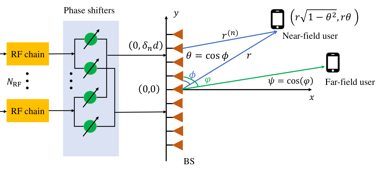
2) Near-field channel model: For the NU, we consider the more accurate spherical-wave propagation model, which applies as well when the user locates in the far-field region. As such, the BS$\to$NU channel can be modeled as

where $h_{\rm near}=\frac{\sqrt{\beta}}{r}e^{-\frac{\jmath 2\pi r}{\lambda}}$ is the complex-valued channel gain³³ 3 In this paper, we consider the Fresnel region with the BS-NU distance $r$ larger than $1.2D$, for which the amplitude variations over XL-array antennas are negligible [9], while the case with non-negligible amplitude variations will be left for future work. with $\beta$ and $r$ denoting the reference channel gain at a distance of $1$ m and the distance between the BS center and the NU, respectively. $\mathbf{b}^{H}(\theta,r)$ denotes the near-field steering vector, which is given by [10]

where $\theta=2d\cos(\phi)/\lambda$ denotes the spatial angle of the NU with $\phi$ denoting the physical AoD from the BS center to the NU; $r^{(n)}=\sqrt{r^{2}+\delta_{n}^{2}d^{2}-2r\theta\delta_{n}d}$ represents the distance between the $n$-th antenna at the BS (i.e., ($0,\delta_{n}d$)) and NU.

The BS is equipped with $N_{\rm RF}\geq K$ radio frequency (RF) chains to enable multiuser communications (i.e., $K$ users). Without loss of generality, we assume $N_{\rm RF}=2$ for the two-user case. Moreover, to facilitate the interference analysis in the sequel, we assume the analog-only beamforming for each user, while the analysis can be extended when digital beamforming is applied to further reduce the interference. Let $x_{k}$, $k=\{1,2\}$ denote the transmitted symbol by the BS to user $k$ with power $P_{k}$, and $\mathbf{v}_{\rm near}$ and $\mathbf{v}_{\rm far}$ represent the transmit beamformers for the NU and FU, respectively. Then, the received signal at the NU is given by

where $z_{0}$ is the received additive white Gaussian noise (AWGN) at the NU with power $\sigma^{2}$.

As such, the receive signal-to-interference-plus-noise ratio (SINR) at the NU is given by

First, with the definitions of $\mathbf{a}(\psi)$ in (2) and $\mathbf{b}^{H}\left(\theta,r\right)$ in (4), the normalized interference power $f(N,\psi,\theta,r)$ can be explicitly expressed as

where $(a_{1})$ follows from the taylor expansion and Fresnel approximation with $r^{(n)}=\sqrt{r^{2}+\delta_{n}^{2}d^{2}-2r\theta\delta_{n}d}\approx r-\delta_{n}d\theta+\frac{\delta_{n}^{2}d^{2}(1-\theta^{2})}{2r}$, and $(a_{2})$ is obtained by replacing $\delta_{n}$ with $n$, i.e., $\delta_{n}=\frac{2n-N+1}{2}$. Note that $(a_{1})$ is accurate when the BS-NU/scatter distance is larger than $0.5\sqrt{D^{3}/\lambda}$, which is much smaller than the Rayleigh distance $2D^{2}/\lambda$.

However, the normalized interference power in (III-A) is still in a complicated form, thus making it hard to characterize the properties of normalized interference power. To tackle this issue, similar to [11], we approximate the normalized interference power in a more tractable form by using Fresnel functions.

Then, the summation in $F(A_{1},A_{2})$ can be approximated as an integral,

where $(b_{1})$ is accurate when $N\to\infty$ according to the Riemann integral, and $(b_{2})$ is obtained by letting $A_{1}n-A_{2}=\frac{\sqrt{2}}{2}t$.

Next, based on the Fresnel integrals, we have

where $\beta_{1}=(\theta-\psi)\sqrt{\frac{r}{d(1-\theta^{2})}}$ and $\beta_{2}=\frac{N}{2}\sqrt{\frac{d(1-\theta^{2})}{r}}$.

By defining $G(\beta_{1},\beta_{2})=\left|F(A_{1},A_{2})\right|$ and combining the above leads to the desired result in (9). $\Box$

To characterize the rate loss due to the FU interference, we first provide the ideal achievable rate of the NU with no interference, which is given by

Then, we define $\Delta_{R}=R^{*}_{\rm near}-R_{\rm near}$ as the rate loss caused by the FU interference, which is upper-bounded as follows.

Lemma 1 is intuitively expected since a higher normalized interference power leads to a larger rate loss $\Delta_{R}$. Combined with the results for the analysis of the interference power, it can be concluded that there is a larger rate loss when the NU and FU angles are very close. However, the analysis for the effects of number of BS antennas and NU distance are not straightforward. For example, when $N$ decreases, it can be shown that $g_{\rm near}$ monotonically decreases, while $f^{2}$ generally increases, leading to a larger $\frac{P_{\rm far}f^{2}}{P_{\rm far}f^{2}+P_{\rm near}}$. Thus, we further provide numerical results in the next to examine these effects.

Last, we show the effects of the four key parameters on the achievable rate of the NU in Figs. 6(a)–6(d) with the simulation parameters shown in Table I. To begin with, we plot in Figs. 6(a) and 6(b) the results based on the used Fresnel approximation in (9) and its actual value in (III-A) versus $N$ and $\psi$. It is observed that the used approximation is highly accurate with the actual value under different $N$ and $\psi$. Second, it is observed from Fig. 6(a) that the rate loss is monotonically decreasing with $N$, which agrees with the result in Lemma 1. An interesting observation is that there still exists a large rate loss when the number of antennas becomes very large (i.e., very low interference power). This is because, with an increasing $N$, the interference power generally decreases, while the beamforming gain (i.e., $g_{\rm near}$ in (14)) increases, thus leading to the performance gap between the achievable and ideal rates of NU. On the other hand, the rate loss fluctuates when the FU angle is in the neighborhood of the NU angle, and drastically decreases when the angle is larger than a threshold (see Figs. 6(b) and 6(c)). Next, in Fig. 6(d), we observe that the rate loss first slightly fluctuates when $r$ is small, and sharply decreases when $r$ increases. Last, it is observed from Figs. 6(b)–6(d) that the achievable rate of NU will eventually approach to the ideal rate when the rate loss is sufficiently small.

References

- [1] M. Cui, Z. Wu, Y. Lu, X. Wei, and L. Dai, “Near-field communications for 6G: Fundamentals, challenges, potentials, and future directions,” IEEE Commun. Mag., early access, 2022.
- [2] Q. Wu, S. Zhang, B. Zheng, C. You, and R. Zhang, “Intelligent reflecting surface-aided wireless communications: A tutorial,” IEEE Trans. Commun., vol. 69, no. 5, pp. 3313–3351, 2021.
- [3] H. Lu and Y. Zeng, “Near-field modeling and performance analysis for multi-user extremely large-scale MIMO communication,” IEEE Commu. Lett., vol. 26, no. 2, pp. 277–281, 2022.
- [4] Y. Zhang, X. Wu, and C. You, “Fast near-field beam training for extremely large-scale array,” IEEE Wireless Commun. Lett., vol. 11, no. 12, pp. 2625–2629, 2022.
- [5] Z. Wu, M. Cui, and L. Dai, “Multiple access for near-field communications: SDMA or LDMA?” arXiv preprint arXiv:2208.06349, 2022.
- [6] C. Sun, X. Gao, S. Jin, M. Matthaiou, Z. Ding, and C. Xiao, “Beam division multiple access transmission for massive MIMO communications,” IEEE Trans. Commun., vol. 63, no. 6, pp. 2170–2184, 2015.
- [7] H. Zhang, N. Shlezinger, F. Guidi, D. Dardari, M. F. Imani, and Y. C. Eldar, “Beam focusing for near-field multiuser MIMO communications,” IEEE Trans. Wireless Commun., vol. 21, no. 9, pp. 7476–7490, 2022.
- [8] C. You, B. Zheng, and R. Zhang, “Fast beam training for IRS-assisted multiuser communications,” IEEE Wireless Commun. Lett., vol. 9, no. 11, pp. 1845–1849, 2020.
- [9] E. Björnson, Ö. T. Demir, and L. Sanguinetti, “A primer on near-field beamforming for arrays and reconfigurable intelligent surfaces,” in 2021 55th Asilomar Conference on Signals, Systems, and Computers. IEEE, 2021, pp. 105–112.
- [10] H. Luo and F. Gao, “Beam squint assisted user localization in near-field communications systems,” arXiv preprint arXiv:2205.11392, 2022.
- [11] N. Deshpande, M. R. Castellanos, S. R. Khosravirad, J. Du, H. Viswanathan, and R. W. Heath Jr, “A wideband generalization of the near-field region for extremely large phased-arrays,” arXiv preprint arXiv:2206.14323, 2022.
- [12] M. Cui and L. Dai, “Channel estimation for extremely large-scale MIMO: Far-field or near-field?” IEEE Trans. Commun., vol. 70, no. 4, pp. 2663–2677, 2022.