Derivation of the wave kinetic equation: Full range of scaling laws
Abstract.
This paper completes the program started in [14, 15] aiming at providing a full rigorous justification of the wave kinetic theory for the nonlinear Schrödinger (NLS) equation. Here, we cover the full range of scaling laws for the NLS on an arbitrary periodic rectangular box, and derive the wave kinetic equation up to small multiples of the kinetic time.
The proof is based on a diagrammatic expansion and a deep analysis of the resulting Feynman diagrams. The main novelties of this work are three-fold: (1) we present a robust way to identify arbitrarily large “bad” diagrams which obstruct the convergence of the Feynman diagram expansion, (2) we systematically uncover intricate cancellations among these large “bad” diagrams, and (3) we present a new robust algorithm to bound all remaining diagrams and prove convergence of the expansion. These ingredients are highly robust, and constitute a powerful new approach in the general mathematical study of Feynman diagrams.
1. Introduction
1.1. Setup and the main result
In this paper we derive the wave kinetic equation, from the continuum cubic nonlinear Schrödinger equation and at the kinetic time scale, for the full range of scaling laws between the large box and weak nonlinearity limits. This completes the program initiated in [13, 14], aiming at providing rigorous mathematical foundation for the wave turbulence theory.
In dimension , consider the cubic nonlinear Schrödinger equation
| (NLS) |
on the square torus of size (all results and proofs extend without change to arbitrary rectangular tori). Here is a parameter indicating the strength of the nonlinearity, and is the normalized Laplacian. We also set the space Fourier transform as
| (1.1) |
where . Note that this convention is different from (but equivalent to) the one in [14, 15]; the parameters in [14, 15] and in the current paper are related by .
Assume the initial data of (NLS) is given by
| (DAT) |
where is a given Schwartz function, and is a collection of i.i.d. random variables. For concreteness, we will assume each is a standard normalized Gaussian.
Define the kinetic (or Van Hove) time
For a fixed value , we will assume that the scaling law between and is , so we have .
1.1.1. The wave kinetic equation
The wave kinetic equation is given by:
| (WKE) |
where is as in Section 1.1, and the nonlinearity is given by
| (1.2) |
Here and below denotes the Dirac delta, and we define
where and are or vectors.
Given any Schwartz initial data , the equation (WKE) has a unique local solution on some short time interval depending on .
1.1.2. The main result
The main result is stated as follows.
Theorem 1.1.
Fix and . Fix a Schwartz function , and fix depending only on . Consider the equation (NLS) with random initial data (DAT), and assume so that .
Then, for sufficiently large (depending on ), the equation has a smooth solution up to time
with probability . Moreover we have
| (1.3) |
where is as in (1.1), and is the solution to (WKE). In (1.3) and below we understand that the expectation is taken under the assumption that (NLS) has a smooth solution on , which is an event with overwhelming probability.
A few comments about this result are in order.
- •
The nonlinear Schrödinger equation (NLS) is studied here and in [13, 14, 15], as a representative model in nonlinear wave theory. In fact, it is the universal Hamiltonian nonlinear dispersive equation, in the sense that any such equation gives (NLS) in a suitable limiting regime [46]. The methods we develop here also apply to other dispersive models modulo technical differences.
- •
Theorem 1.1 holds for the rectangular torus for any (rational or irrational) without genericity assumption. Here we only present the proof for the square torus, but the general case can be treated by the same arguments.
- •
In the same way as [14], the assumption that is Schwartz is unnecessary. In fact it suffices to assume that its first derivatives decay like . Moreover the error term defined in (1.3) enjoys the explicit decay rate , which is uniform in and , for some absolute constant . The value of we get, though, is likely non-optimal.
- •
- •
The main results in [15] (evolution of higher order moments, propagation of chaos, law evolution for non-Gaussian data, derivation of wave kinetic hierarchy) also extend to the current setting. In particular, we can replace the i.i.d. Gaussians by any centered-normalized i.i.d. random variables whose law is rotationally symmetric and has exponential tails. This is easily shown by combining the arguments in this paper and in [15] with obvious modifications.
1.2. Background and literature
The theory of wave turbulence describes the non-equilibrium statistical behavior of systems of interacting waves, in the thermodynamic limit where the number of degrees of freedom goes to infinity. It is the wave analog of the classical kinetic theory of Boltzmann for particles, and its rigorous justification corresponds to the Hilbert’s sixth problem for nonlinear waves.
The basic setup of the theory is as follows. Start with a nonlinear dispersive equation as the microscopic system of nonlinear waves. This is (NLS) in our case, but can also be replaced by other equations. Such system is studied in a large box with a weak nonlinearity , where (so the number of degrees of freedom diverges as ) and in the limit. Assume the initial data is random and well-prepared as in (DAT), i.e. the different Fourier modes are independent and satisfy a random phase (RP) condition. Then, among other things, the following kinetic description is expected at the kinetic time :
- •
Propagation of chaos: different Fourier modes should remain independent in the limit;
- •
The wave kinetic equation: the evolution of energy density should be governed by (WKE) in the limit.
In the physics literature, the very first kinetic description for waves appeared in Peierls [38] in the study of anharmonic crystals, leading to the so-called phonon Boltzmann equation. Since then, the kinetic theory has been developed for various models, and has become a systematic paradigm starting in the 1960s, with immense applications in various fields of physics and science [2, 3, 12, 29, 30, 32, 36, 43, 44, 47, 48, 49]. The name wave turbulence theory comes from the spectral energy dynamics and cascades that the wave kinetic equation predicts for nonlinear wave systems, which yields similar conclusions to Kolmogorov spectra in hydrodynamic turbulence; this connection was is a major contribution of Zakharov [50, 51].
On the other hand, the rigorous mathematical treatment of wave turbulence had to wait until much later for the appropriate conceptual and technical ingredients to be invented. While it was clear in the theoretical physics community that a Feynman diagram expansion is the right approach to the problem, the main mathematical issue here was to prove the convergence of such an expansion. Naturally, the progress started in a linear setting (e.g. electron moving through random impurities), namely with the work of Spohn [41] for short kinetic times. This was later extended to much longer times in the celebrated works of Erdös-Yau [20] and Erdös-Salmhofer-Yau [21]. Obviously, the next level of progress is to advance this understanding to the nonlinear setting, where the randomness is only coming from the initial distribution of the data as explained in [42]. The first breakthrough proving the convergence of the diagrammatic expansion in a nonlinear setting was that of Lukkarinen-Spohn [33], which considered the lattice (NLS) and studied the time correlations of the invariant Gibbs measure in the thermodynamic limit. Even though the above works only dealt with linear or equilibrium settings, they managed to draw substantial interest to this field from the mathematical community, and inspired subsequent research. In the last decade, partial results have been proved regarding the derivation of (WKE) in the nonlinear out-of-equilibrium setting, starting with works that addressed certain aspects of the problem (second-order expansions, near-equilibrium dynamics, shorter time scales etc.), see [8, 10, 11, 13, 18, 19, 24] and references therein. In particular, the authors’ earlier work [13], as well as Collot-Germain [10, 11], provides the justification of (WKE) up to the almost sharp time scale for any .
In April 2021, the authors [14] completed the first rigorous derivation of (WKE) up to time for scaling laws or close to . Subsequently, propagation of chaos and other predictions of wave turbulence theory were proved in [15]. This includes the asymptotics of higher order correlations, derivation of the wave kinetic hierarchy, limit equations for the law of when the initial distribution is not necessarily Gaussian, and propagation of Gaussianity in the case the initial distribution is Gaussian.
We should mention that, after the work [14], some other results in a similar vein were also obtained, but for equations with special time-dependent random forcing. In [45], Staffilani and Tran derived the wave kinetic equation for the Zakharov-Kuznetsov equation in the presence of a time-dependent noise that provides an additional randomization effect for angles in Fourier space. Recently they extended their result to the spatial inhomogeneous setting with a different noise, in joint work with Hannani and Rosenzweig [28]. At this time, [14, 15, 28, 45] are the only results that reach the kinetic time in the non-equilibrium setting. Some more recent results that cover shorter time scales, but do not include forcing, can be found in [1, 35].
In addition to the derivation of (WKE), there are also many works devoted to the study of the behavior of solutions to wave kinetic equations like (WKE), see for example [9, 22, 23, 26, 39, 40]. This is another very important question, but is less related to the focus of this paper, so we will not elaborate on its state of art here.
1.3. The scaling laws
Note that the kinetic description of wave turbulence theory involves the two limits and . In fact, it is very important to specify the exact manner in which these two limits are taken. The most general form of such limits would be
for some , which is called a scaling law. Note that, the endpoint case is understood as the iterated limit where first with fixed and then ; the case is the opposite. The purpose of this section is to explain the necessary conditions on the scaling laws for a kinetic theory to hold. This will justify why is the full range of scaling laws for (NLS) on the square torus.
To the best of our knowledge, the role of the scaling law in wave turbulence theory has not been adequately clarified in the physics literature, prior to the recent rigorous mathematical studies. In fact, this was one of the contribution of the authors’ recent works, and is explained clearly in the expository paper [16]. For completeness of the discussion, we elaborate on this here as well.
First of all, not all scaling laws11 1 A common knowledge in physical literature is that the limit should not be taken before the limit (see Remark 1.2), which excludes the scaling law . This may lead to some mistaken belief that the only other option is , i.e. to take first followed by . In fact, as we shall see in Section 1.3.3, the latter is also not compatible with equations on continuum domains, so in continuum setting one has to restrict to scaling laws . In the discrete setting, the scaling law is compatible. allow for the kinetic description in Section 1.2. To see this, consider the equation (NLS) with initial data (DAT), but with a general dispersion relation instead of . Then admits an expansion with the first term being , and (part of) the second term being
| (1.4) |
where , due to a calculation of Duhamel iterations. At time , and when and , this expression formally matches one of the terms in the second iteration of (WKE) (cf. the first term in (1.2)), using the fact that as .
In order for this formal approximation to be legitamite, the one and only restriction is that the values of , as range over the lattice , must be equidistributed at scale . In fact, suppose , then the convergence of (1.4) is intimately tied to the bound
| (1.5) | ||||
The bound (1.5) follows from the convergence of (1.4), if we replace the function by a cutoff function, and similarly for . This means that the probability of a lattice point in falling into the set —the level set of the function —is proportional to the volume of , which is exactly equidistribution of .
Another implication of the equidistribution property (1.5) is that
| (1.6) |
where is defined as above but with . In fact, the sets and are referred to as sets of quasi resonance and exact resonance by physicists, and the latter inequality just states that the contribution of exact resonances should be dominated by volume-counting estimates of quasi resonances in (1.5). This is certainly necessary for the kinetic formalism to hold, and is consistent with the discussions in the physical literature.
1.3.1. Admissible scaling laws
We say a scaling law is admissible, if the above equidistribution property holds for (equivalently in (1.5)). Clearly, the range of admissibility depends on the precise properties of the dispersion relation . Note that a sufficient condition is given by
which corresponds to [36, 27]: in this range, the equidistribution property holds for any reasonably behaved dispersion relation without the need for any number theoretic arguments.
However, for a given (or a class of) dispersion relation , the above sufficient condition is usually not necessary. Specifying to the Schrödinger case (NLS), one can see in multiple ways that the admissible range is in fact for arbitrary (including square) tori, and for tori satisfying a genericity assumption. For example, for the square torus one has , so cannot be equidistributed at scales . Alternatively, the cardinality of the exact resonance set can be shown to be for square tori and under genericity assumption, which leads (using (1.6)) to the same range of . In fact, we shall see that different values of or represent a range of different physical and mathematical phenomena; see Section 1.3.2 for two special cases.
For , the results of the authors’ earlier work [14] covers the range of scaling laws for arbitrary tori, where is a small dimensional constant, as well as under a genericity assumption. The goal of the current work, as stated in Theorem 1.1, is to extend the results to the full range (we discuss the endpoint in Section 1.3.3).
1.3.2. Two important scaling laws
For the Schrödinger equation (NLS), there are two scaling laws of particular mathematical and physical interest. The first one is , so that and . This is consistent with the natural parabolic scaling for (NLS), by which solutions to (NLS) on torus of size and at time scale can be rescaled to solutions on the unit torus and at time ; namely, if solves (NLS) and with , then solves the equation . This means that, the predictions of wave turbulence theory under this scaling law, can be translated into conclusions on the unit torus. In three dimensions, this is closely related to the famous Gibbs measure invariance problem for cubic NLS (i.e. invariance of the measure under the Schrödinger dynamics), which is the only Gibbs measure invariance problem that still remains open after the works [4, 5, 7, 17, 37, 52]. In addition, energy cascade behavior for NLS can also be observed at the level of (WKE) [23, 36], and proving such cascade dynamics for the NLS equation on the unit torus is a problem of great interest [6].
Another important scaling law is for which . We may call this the ballistic scaling law because it equates the kinetic timescale with the ballistic timescale needed for a wave packet at frequency to traverse the domain . In some sense, this is analogous to the Boltzmann-Grad scaling law adopted in Lanford’s theorem justifying the Boltzmann equation, in which the so-called mean-free path is also equated to the transport length scale.
It should be pointed out that such wave packet considerations are more relevant in the inhomogeneous setting of the problem, where the initial field is not homogeneous in space as in (DAT). An example of such data is when one sets (NLS) on with random data whose Wigner transform
| (1.7) |
possibly in a weak sense, where decays rapidly in and . This is achieved, for example, by setting the random data as
| (1.8) |
which can be viewed as an inhomogeneous generalization of that in (DAT). Then, the solution to (NLS) has the form
| (1.9) |
Denoting , which corresponds to the Wigner transform of , and performing a formal expansion, we find that satisfies
| (1.10) |
This gives the inhomogeneous wave kinetic equation provided one equates the transport timescale with the kinetic timescale , which is the scaling law with .
Note that, if one wants to view the homogeneous WKE as a limit of the inhomogeneous one, then one has to introduce an additional parameter to the data in (1.8), namely one measuring the scale of the inhomogeneity. This can be done by rescaling , or equivalently by replacing with in (1.8), where is the new inhomogeneity scale. This leads to the flexibility of scaling laws in the homogeneous setting; in fact all the admissible scaling laws described above arise as suitable limits with and .
1.3.3. The scaling law
Note that Theorem 1.1 covers the full range of scaling laws , except the endpoint . This endpoint does not seem to be compatible with the continuum setting; indeed, formally taking the first will lead to (NLS) on with initial data
which is a Gaussian random field with covariance operator that has uniform strength at every point of . In particular, this initial data, and any possible remainder term that may occur, belongs only to (with logarithmic growth at infinity). However, for data, there is no known solution theory to (NLS) (or even the linear Schrödinger equation) in any function space, due to infinite speed of propagation and the unboundedness of the linear propagator .
Nevertheless, in the discrete setting where is replaced by a discrete difference operator, it is completely plausible to solve (NLS) in (weighted) , so in this case is a compatible scaling law, and the corresponding justification of (WKE) for may be possible [34].
Remark 1.2.
In some early physical literature, the limiting procedure was described as “the limit should be taken before the limit, and not after”. This should not be understood as these two limits being taken independently; rather, it simply means that the rate should not be slower than that of . In other words, we must have , or in the context of scaling laws, where is a constant depending on the setting of the problem. This is clearly consistent with all the above discussions.
1.4. Ingredients of the proof
We briefly describe here the main difficulties and new ingredients in the proof of Theorem 1.1; see Section 3 for a more substantial description, as that requires the notations set up in Section 2.
While the general methodology here follows that in [14] which dealt with the scaling law , fundamentally new structures and ideas appear for scaling laws as we shall explain below. The analysis of these new structures requires introducing new ideas to isolate, analyze, and uncover novel cancellations between some of them. Moreover, it requires upgrading our previous combinatorial algorithm to a much more robust and streamlined apparatus.
The first steps of the proof of Theorem 1.1 are essentially the same as in [14]: one expands the solution to (NLS) into terms indexed by ternary trees, which allows to express the correlations of these terms using couples. These couples (which are the Feynman diagrams in this game) are pairs of trees whose leafs are completely paired to each other. The analysis of such couples goes through parallel analytical and combinatorial approaches. The leading couples, which we call regular couples, are studied and computed analytically to isolate from them the iterates of (WKE). It then suffices to show that the contribution of non-regular couples is of lower order. Here, the novel idea of molecules was introduced in [14] to study the combinatorial problems associated with non-regular couples. This molecular picture will prove to be even more indispensable in this paper.
The same algorithm used in [14] to analyze these molecules breaks down, as soon as . On a superficial technical level, this is due to the failure of a particular two-vector counting estimate (namely the case of (3.2)). However, this break down is much more fundamental and cannot be saved by simply modifying the algorithm. Indeed, when , the molecule may contain new bad structures (in fact multiple families of them) other than those already observed in [14]. Such bad structures are harmless at scaling laws , but can overtake the leading terms for . Note that this difficulty is of very different nature from that of [14], which mainly revolves around overcoming the factorial divergence caused by generic molecules. While this is still a problem here, the extra difficulty imposed by these special bad structures requires substantially new ideas beyond the proof in [14].
The strategy here is to first (i) identify all the possible bad structures—there are eight families of them that we call vines (Figure 16), then (ii) recover a good estimate for any molecule absent of these bad structures (in the form of a rigidity theorem similar to Proposition 9.10 of [14]), and finally (iii) control the contribution of these bad structures.
Parts (i)–(ii) can in fact be done together at the level of the molecule picture, by introducing a powerful new operation that is absent in the algorithm of [14], called the cutting operation (Figure 2). This seemingly simple operation allows us to isolate all the possible bad scenarios into “local” post-surgery connected components, and locate only finitely many families of connected components that are problematic. It is precisely this small addition that leads to the complete classification of bad structures in this paper, namely the vines. We believe that this is the one missing piece in the algorithm of [14] that makes it much more robust. We also notice that the combinatorial difficulty caused by vines is not specific to the (NLS) case, but is actually universal (at least in the -wave setting) independent of dispersion relation and multilinear multipliers. As such, we believe that the algorithm in [14], equipped with the cutting operation, should be directly applicable in many other settings.
Part (iii) of this plan, which is another main novelty of this work, relies on extremely delicate, and somewhat miraculous, cancellations observed between the bad structures identified in (i). Indeed, starting from these bad structures identified at the level of the molecule, one can reconstruct the various possibilities of couples that have this same molecular structure. These couples, which may have arbitrarily large size, can be grouped into pairs defined as twists of each other (Figures 6 and 18). The cancellation structure is then found by studying expressions associated with couples that are twists of each other. It is worth mentioning that this cancellation is so involved and intricate that there is little-to-no chance of uncovering it if one only looks at the couple picture, and does not turn to the molecule picture (cf. Figure 8). This strongly suggests that the molecules introduced in [14] are fundamental objects, and not mere technical tools.
To the best of our knowledge, the cancellation identified in this paper has not appeared in earlier mathematical or physical literature (such structures only become significant in higher oder terms, so it’s not surprising that they do not play a role in the formal derivation of physicists that only involve second order expansions). Therefore, we believe that the ingredients of this paper and [14]—including cancellations of vine structures and the algorithm in [14] with cutting—constitute the next major step beyond [20, 21, 33] in the study of Feynman diagrams. This development allows us to effectively estimate diagrams of much higher order than those in [20, 21, 33], which results in the proof of Theorem 1.1 in the non-equilibrium setting and without noise.
Finally, we remark that, this new Feynman diagram analysis is robust enough to be applicable in a wide range of semilinear dispersive equations. The only major difference for other dispersion relations would be the equidistribution property (1.5), which may restrict the range of scaling laws depending on the fine number theoretic properties of . However, these number theoretic ingredients are only needed when ; for , we expect that results like Theorem 1.1 should hold for arbitrary , as demonstrated in Section 1.3.1.
1.5. Future Horizons
We conclude this introduction by listing, what we believe to be some of the next major frontiers in this line of research, after the resolution (here and in [14, 15]) of the first fundamental question that is the rigorous justification of the wave kinetic theory.
(1) Longer times: the obvious question after Theorem 1.1 would be whether the same result can be extended to time for constants . This is a tremendous open problem, and its resolution is unknown not only in the wave turbulence setting, but also in the classical particle setting of Lanford’s theorem justifying Boltzmann’s equation. Note that (WKE) may have finite time blowup (which is even expected to be generic, see [22, 23]), so the best one can hope for, in terms of the approximation (1.3), would be the following conjecture:
- •
Answering this conjecture is highly challenging, and would require ideas and techniques completely different from the current and earlier works. Moreover, a positive answer would have profound implications on the study of long-time dynamics of (NLS), especially on energy cascades.
(2) Post-singularity dynamics: Suppose that the conjecture in (1) has been proved or is assumed to be true. Moreover, suppose a specific solution to (WKE) exhibits a singularity at a particular time . The analysis in [22, 23] suggests that such singularity formation is somewhat generic (formation of condensate). Then we may ask the following question: what is the asymptotic behavior of
In other words, can one prove rigorously the dynamical formation of condensate for (NLS)? More interestingly, for , can one still track the macroscopic behavior of ? Does it converge to a finite limit? If so, can it be defined as a weak solution to (WKE) in some sense? If not, then should we somehow modify (NLS) (and/or the wave kinetic equation) beyond the time , in view of the condensate formed for (WKE) at ? These questions may be even more challenging than the conjecture in (1), but their resolution would bring new insights, both physical and mathematical, to the study of (NLS) and its condensates.
(3) Properties of solutions to (WKE): turning now to the solution theory to (WKE), an important question is to describe more precisely the formation of condensate [22, 23], and perhaps justify its genericity, for sufficiently strong classes of solutions. Another venue of immense physical interest, is to rigorously study solutions that may asymptote to (or resemble in some meaningful sense) the Zakharov spectra, see for example [9] for a step in this direction. These specific solutions, when combined with possible results in (1) and (2), may lead to the discovery of very interesting behavior of solutions to (NLS).
One may also consider the inhomogeneous version of (WKE), whose derivation is expected to be similar to (WKE) with only technical differences. However, solutions to the inhomogeneous (WKE) may behave quite differently, for the transport term may prevent blowup. If these solution exhibit diffusive behavior for long times, this may lead to a nonlinear version of the quantum diffusion behavior described in Erdös-Salmhofer-Yau [21] in the linear setting.
1.6. Acknowledgements
The first author is supported in part by NSF grant DMS-1900251 and a Sloan Fellowship. The second author is supported in part by NSF grant DMS-1654692 and a Simons Collaboration Grant on Wave Turbulence. The authors would like to thank Herbert Spohn for several discussions, that explained the importance of other scaling laws (particularly ). This was a major drive to study the full range of scaling laws in this paper. The authors also thank Jani Lukkarinen for explaining the work [33] and several other illuminating discussions.
2. Preparations
2.1. Preliminary reductions
Start from the equation (NLS), let be a solution, and recall . Let be the conserved mass of (where takes the average on ), and define , then satisfies the Wick ordered equation
| (2.1) |
By switching to Fourier space, rescaling in time and reverting the linear Schrödinger flow, we define
| (2.2) |
with as in (1.1), then will satisfy the equation
| (2.3) |
with the nonlinearity
| (2.4) |
for . Here in (2.4) and below, the summation is taken over , and
| (2.5) |
and the resonance factor
| (2.6) |
Note that is always supported in the set
| (2.7) |
2.2. Parameters, notations and norms
In this subsection we list some notations and fix some parameters that will be useful below. Recall that and , and Schwartz data are fixed. Define
| (2.8) |
Fix as a small absolute constant such that , and let be any large constant depending on and . Let also be any large constant depending on and , and fix as a small constant such that . Unless otherwise stated, the implicit constants in symbols may depend on , but those in symbols depend only on . Let be large enough depending on , and define .
Let be such that for and for ; define and , where are coordinates of vectors (we use this notation throughout). By abusing notation, sometimes we may also use to denote other cutoff functions with slightly different supports. These functions, as well as the other cutoff functions, will be in Gevrey class (i.e. the -th order derivatives are bounded by ). For a multi-index , we adopt the usual notations and , etc. For an index set , we use the vector notation and , etc.
Denote for a complex number , and . In the rest of this paper, we will not use the space Fourier transform notation as in (1.1). We will use only for the time Fourier transform, which is defined as
and similarly for higher dimensional versions. If a function depends on several time variables and several vector variables , we shall define its norm by
If does not depend on any , the norms are modified accordingly; they do not depend on so we call it . Define the localized version , and associated auxiliary norm, by
If we will only use the value of in some subset (for example , see the second part of Proposition 6.1), then in the above definition we may only require in this set. Finally, define the norm for function ,
| (2.9) |
All these norms are readily extended to Banach space valued functions.
2.3. Trees, couples and decorations
Recall the notions of trees, couples and decorations, which are defined in [14].
Definition 2.1 (Trees).
A ternary tree (we will simply say a tree below) is a rooted tree where each non-leaf (or branching) node has exactly three children nodes, which we shall distinguish as the left, mid and right ones. A node is a descendant of a node , or is an ancestor of , if belongs to the subtree rooted at (we allow ). We say is trivial (and write ) if it has only the root, in which case this root is also viewed as a leaf.
We denote generic nodes by , generic leaves by , the root by , the set of leaves by and the set of branching nodes by . The order of a tree is defined by (this is called scale in [14]), so if then and .
A tree may have sign or . If its sign is fixed then we decide the signs of its nodes as follows: the root has the same sign as , and for any branching node , the signs of the three children nodes of from left to right are if has sign . Once the sign of is fixed, we will denote the sign of by . Define . We also define the conjugate of a tree to be the same tree but with opposite sign.
Definition 2.2 (Couples).
A couple is an unordered pair of two trees with signs and respectively, together with a partition of the set into pairwise disjoint two-element subsets, where is the set of leaves for , and where is the order of . This is also called the order of , denoted by . The subsets are referred to as pairs, and we require that , i.e. the signs of paired leaves must be opposite. If both are trivial, we call the trivial couple (and write ).
For a couple we denote the set of branching nodes by , and the set of leaves by ; for simplicity we will abuse notation and write . Define . We also define a paired tree to be a tree where some leaves are paired to each other, according to the same pairing rule for couples. We say a paired tree is saturated if there is only one unpaired leaf (called the lone leaf). In this case the tree forms a couple with the trivial tree . Finally, we define the conjugate of a couple as with the same pairings; for a paired tree we also define its conjugate as with the same pairings, where is as in Definition 2.1.
Definition 2.3 (Decorations).
A decoration of a tree is a set of vectors , such that for each node , and that
for each branching node , where is the sign of as in Definition 2.1, and are the three children nodes of from left to right. Clearly a decoration is uniquely determined by the values of . For , we say is a -decoration if for the root .
Given a decoration , we define the coefficient
| (2.10) |
where is as in (2.5). Note that in the support of we have that for each . We also define the resonance factor for each by
| (2.11) |
A decoration of a couple , is a set of vectors , such that is a decoration of , and moreover for each pair . We define , and define the resonance factors for as in (2.11). Note that we must have where is the root of ; again we say is a -decoration if . We also define decorations of paired trees, as well as and etc., similar to the above (except that we don’t pair all leaves).
2.4. The ansatz and main estimates
We now state the ansatz for the solution a to the system (2.3)–(2.4), as well as the main estimates.
2.4.1. The expressions and
For any tree of order , define the expression
| (2.12) |
where the sum is taken over all -decorations of , and the domain
| (2.13) |
For any couple of order , define the expression
| (2.14) |
where the sum is taken over all -decorations of , the product is taken over all leaves with sign, and the domain
| (2.15) |
2.4.2. The ansatz for
Let
| (2.16) |
where the sum is taken over all trees of order and sign , and define by
| (2.17) |
where as defined in Section 2.2. Then b satisfies an equation of form
| (2.18) |
or equivalently
| (2.19) |
where the relevant terms are defined as
| (2.20) |
and . The sums in (2.20) are taken over , each of which being either b or for some . In the sum for , exactly inputs in equals b, and in the sum we require that with . Note that , and are -linear, -bilinear and -trilinear operators respectively.
2.4.3. Correlations, and expansion of (WKE)
For any , by using Isserlis’ theorem as in Section 2.2.3 of [14], we have that
| (2.21) |
where the summation is taken over all couples such that and (the partition can be arbitrary).
2.4.4. The main estimates
The followings are the main estimates of this paper. Their proofs will occupy up to Section 11.1; once they are proved, Theorem 1.1 will then be proved in Section 11.2, similar to Section 12 of [14].
Proposition 2.4.
Let be defined in (2.14). Then for each , and we have
| (2.24) |
where the summation is taken over all couples such that .
Proposition 2.5.
Let be defined as in (2.23). Then for each , and , we have that
| (2.25) |
where the summation is taken over all couples of order . If is replaced by , then the same result holds with replaced by .
Proposition 2.6.
For any -linear operator define its kernel (which we assume is supported in and ), where , such that
| (2.26) |
Now let be defined as in (2.20). Then there exists an -linear operator , and and , such that
| (2.27) |
The kernels of , and are Weiner chaos of order , and they satisfy that
| (2.28) |
for any and and with . The same holds for and and any .
Remark 2.7.
Recall that the support of the coefficient in (2.5), which is the set in (2.7), allows for the degenerate case . However in this case we must have , and such case is always easily treated (see for example Section 9.3.1 of [14] which deals with degenerate atoms).
For simplicity of presentation, we will neglect the degenerate case for most of this paper and assume that is always supported in the set where . In Section 10.5 after the main proof, we briefly discuss how to treat degenerate cases, which only requires minor modifications.
3. Overview of the proof
3.1. Previous strategy, and the main difficulty
Let us start from the proof of Propositions 2.4 and 2.5, which requires us to analyze the quantity . The early steps in the analysis are essentially the same as in [14] (which deals with the case ). First one identifies and analyzes the leading couples, called regular couples, which are ones built by concatenating specific building blocks called mini couples (cf. Definition 4.8 and Figure 10). The analysis of those couples was done in [14] and is basically independent of the chosen scaling law. As such, the heart of the matter is showing that the contribution of non-regular couples is lower order. The analysis of non-regular couples proceeds by applying a structure theorem (Proposition 4.9) to reduce to prime couples (Section 6.3), which are couples that contain no regular sub-couples inside them. Then, one uses the almost bound for the time integral in (6.48) (see for example (8.13)) to reduce the estimates on such prime couples to a counting problem for decorations of , which has the form
| (3.1) |
in the notions of Definition 2.3.
To study the counting problem, we then introduce the notion of molecules (Definition 4.2), which is of fundamental importance in [14] and even more so in the current paper. Basically, a molecule is a directed graph formed by atoms which are -element subsets as in (3.1), and bonds which are common elements of these subsets under the given pairing structure; such a molecule coming from a couple will have all degree atoms except for exactly two degree atoms, and moreover contains no triple bond if the couple is prime. The system (3.1) is then reduced to a system for decorations this molecule (Definition 4.6), where each bond is decorated by a vector and each atom gives an equation of form (3.1) with variables corresponding to the bonds at this atom. As a central component of the proof, we need to establish a suitable rigidity theorem, which (schematically) states that
- •
Apart from some explicitly defined special structures, the counting problem provides sufficient control for , with an additional power gain22 2 This extra gain is needed to cancel the factorial divergence coming from the number of generic couples and molecules, which is the major difficulty in [14]. Exactly the same gain is needed also in the current work. proportional to the size of the molecule .
It is at this point that the arguments for and start to differ, and the new structures and ideas start to emerge.
3.1.1. The case
When (and similarly when ), the counting problem for the molecule is solved by designing a reduction algorithm (Section 9.4 of [14]), where in each step we remove one or two atoms and their bonds, and reduce to the counting problem for a smaller molecule. Each such operation is either good and favorable for counting (i.e. the desired bound for the smaller molecule implies strictly better than desired bound for the original molecule) or normal and neutral for counting (i.e. the desired bound for the smaller molecule implies precisely the desired bound for the original molecule). Note that there is no bad operations, and the proof goes by a careful analysis of the algorithm, using suitable invariants and monotonic quantities, that shows at least a fixed small portion of all operations are good, apart from two special structures called type I and II molecular chains.
As for the special structures, type I chains are formed by double bonds only; type II chains are formed by single and double bonds (the lower right corner of Figure 16), and in the current paper we will refer to them as ladders. These ladders are neutral for counting, and their presence does not help or harm anything, so we will mostly ignore them for the rest of this section. In comparison, type I chains cause a logarithmic loss when , but this is compensated by a delicate cancellation between different type I chains (which come from irregular chains in the corresponding couples), see Section 8.3 of [14]. Such cancellation was previously unknown in either mathematical or physical literature, and is another key component of the proof in [14].
3.1.2. The case: Main difficulties
We now turn to the general range . In fact, the most typical case, and in some sense the hardest case, is the ballistic scaling . For simplicity, we will assume this scaling for the rest of this section.
Recall that in [14], when , the key quality of the operations in the algorithm—namely good and normal—relies on what we may call the atomic counting estimates, which involve one or two atoms (i.e. systems similar to (3.1)), and between and bonds (i.e. unknown vectors). For example, favorable - and -vector counting estimates take the form
| (3.2) |
for and fixed; the - and -vector counting estimates involve two systems, see Lemma A.3 (3) and (4).
Now, when , we can prove the same (good and normal) bounds for the -, - and -vector counting problems just as in the case; however, the two vector counting bound, namely (3.2) with , breaks down. Indeed, in the worst case scenario , the left hand side of (3.2) is of order which loses compared to (3.2).
This, being the only difference between the and cases, seems to be a minor issue at first sight; however it turns out the have a huge effect on the analysis of molecules. First of all, this leads to the presence of bad operations in the algorithm (say when one removes one atom of degree ), where the desired bound for the smaller molecule does not imply the desired bound for the original molecule, so the approach in [14] breaks down; in fact it breaks down in a much more essential way, due to the occurrence of new bad special structures.
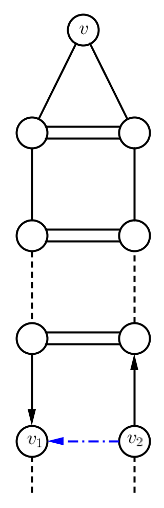
Of course, the double bond chain—called type I chain in [14]—are now quite bad in terms of counting, but as in [14] they are compensated by cancellation, albeit in a slightly more subtle manner. Nevertheless, there are families of much more complicated structures, which are favorable for counting when , but becomes bad when , for example the one shown in Figure 1. Moreover, there are also six more families of structures which are favorable for counting when , but become neutral when . These are depicted in Figure 16, including the one in Figure 1, and are collectively referred to as vines.

This means that, even in the statement of the rigidity theorem, one has to exclude, in addition to double bond chains and ladders, all the different vines as well as chains formed by them. Dealing with these new structures is the major challenge (which we discuss further in Section 3.3), but even if we assume absence of these vines, it is not at all clear why the rigidity theorem would hold. In particular, the vines occurring in Figure 16 seem sporadic and unrelated to each other, so how can we identify them from all the other structures and show they are the only bad ones?
All these considerations have led to an important modification to the algorithm, namely the addition of a new operation called cutting. This not only makes the algorithm in [14] much more robust, but also allows one to naturally see the occurrence of all the vines in Figure 16, which would otherwise seem to be coming from nowhere. We shall elaborate on on this further below.
3.2. Vines, derived from cutting
Now we discuss the main new ingredient in our modification to the algorithm in [14], namely the new operation called cutting.
Recall that the only bad operation that can ever occur in the algorithm is -vector counting, and this typically come from removing a degree atom , which has two bonds of opposite directions, such that as in (3.2) with . Suppose has degree before any operation (i.e. in the original molecule), then due to the first equation in (3.1), the other two bonds at must also satisfy . We then call such atoms a small gap, or SG atom. In comparison, assume (under a small simplification) that all other atoms with bonds must have that for any pair of opposite directions, and call them large gap or LG atoms.
Therefore, it is the SG atoms that will cause bad operations to occur, and such bad operations are hard to control once they enter the main algorithm. To isolate the difficulties, the natural idea is then to get rid of these potentially bad atoms in the first place, before entering the algorithmic phase. The precise operation we perform in this pre-processing stage is cutting. As its name suggests, at each step we choose a degree SG atom , and split it into two atoms of degree , as in Figure 2 below (see also Figure 22).

There are two cases of cutting: when this operation does not create a new connected component (which we call -cutting, see Definition 9.3), or when it creates a new connected component (which we call -cutting). It turns out that cuttings are favorable for counting in a certain sense, and leads to power gains instead of losses, so below we will focus on -cuttings.
3.2.1. Local rigidity theorems
Suppose we have done all possible cuttings (say they are all -cuttings), then the resulting graph is composed of finitely many connected components. A typical component will contain several degree atoms that result from cutting, as well as degree atoms33 3 There is only one component with two degree atoms, which enjoys much better estimates compared to other components, and will be neglected in the discussions below.; the point here is that all the degree atoms must have large gap, and so will not be involved in any bad operations. Moreover, since the number of degree atoms and the number of components satisfy , we expect that a typical component will contain exactly two degree atoms. We will fix such a component below.
Before getting to the counting problem, we shall make one more reduction to this component. For each degree atom , suppose it has two bonds , then we may remove and these two bonds, and replace them by a single bond connecting their two other endpoints. If this operation introduces a new triple bond, then we may further remove the two endpoint atoms of this triple bond and add one new bond between the two other atoms connected to these two endpoints, and keep doing so until no more new triple bonds appear. The combined effect of this sequence of operations, which we may call the (Y) sequence, is shown in Figure 3. Let the graph resulting from this sequence be . Note that this sequence essentially corresponds to removing a degree atom together with a ladder attached to it, and recall that ladders are neutral objects for counting. In fact, this sequence is also neutral for counting, in the sense that each decoration of provides also a decoration of , and the desired bound for the counting problem for implies precisely the desired bound for the counting problem for .
Now the goal is to study the counting problem associated with ; let the number of solutions to this counting problem be , and let be the characteristics of (where and are number of bonds and atoms in , and is the number of components which is for now). We would like to compare with the quantity , and thus define . Then, the main result for can be stated in the form of a “local” rigidity theorem (Proposition 9.6, see also Proposition 10.4), as follows:
- •
If does not equal to one of the finitely many explicitly defined “bad” graphs, then, apart from ladders, we have for some constant .
The proof of the local rigidity theorem, as well as the arguments leading to the bad graphs, relies on the exact algorithm described in Section 9.4 of [14]; of course this is owing to the fact that we no longer have any SG atoms in . However there is also price to pay, namely that now a typical component contains only degree atoms, as opposed having two degree atoms before doing all the cuttings. Therefore, the first step in the algorithm necessarily have to be removing a degree atom, which corresponds to a counting problem of form (3.2) but with (note this is different from the -vector counting in Lemma A.3 (2)). This is one—but the only one—bad operation in the algorithm, which loses power , in the sense that the value before the operation is only bounded by times the value after the operation.
After this first bad operation, we no longer need to consider (3.2) with , so the remaining operations are all good or normal, due to absence of SG molecules; in summary, we have one bad operation per component (as opposed to potentially many bad operations due to SG atoms, had we not done the cuttings in the first place). Moreover, it can be shown that each good operation gains power (opposite to the above, so that the value before the operation is bounded by times the value after the operation). A subsequent discussion, in the same spirit as Section 9.5 of [14], then allows us to bound the number of good operations from below. More precisely, apart from ladders, there is only one case for in which there is no good operation (so ), namely when is a quadruple bond; there is also only one case for in which there is exactly one good operation (so ), namely then is a triangle of three double bonds. These are shown in Figure 4. In all the other cases, the number of good operations is at least two, so we have . If we choose small enough, this already proves the local rigidity theorem when ; if , then we can repeat the proof in Section 9.5 of [14]—almost word by word—to get that the power gain is at least proportional to the size of the graph, which makes the loss in the only bad operation negligible. In the end, this allows us to prove the local rigidity theorem.

3.2.2. Vines
With the local rigidity theorem proved, we only need to check all the possibilities for components with exactly two degree atoms, which lead to the two bad cases—a quadruple bond and a triangle of three double bonds—after at most two (Y) sequences described above. These possibilities can be found by enumeration, and exactly correspond to the families of vines (II)–(VIII) (except vines (I) which are double bonds) in Figure 16; in fact, this is exactly how these vines are discovered. The following Figure 5 shows an example of how a specific case of vine (VI) is reduced to a triangle of three double bonds after two (Y) sequences; the other cases can be shown similarly (see the proof of Lemma 10.5).
It is now easy to get the main rigidity theorem, namely Proposition 8.6, by combining the local rigidity estimates for all components after cutting; however, we still need to analyze the vines. In fact, vines (III)–(VIII) in Figure 16 are neutral for counting, and do not cause any gain or loss in powers; nevertheless, each individual vine (I) or (II) would cause a serious power loss. These will be controlled, by some surprisingly delicate cancellations, which we discuss next.

3.3. The miraculous cancellation
As described above, we are now left with the analysis of vines (I) and (II) (called bad vines) in Figure 16. Since double bonds are essentially the same as in [14], we will focus on vines (II) in this subsection.
To exhibit the cancellation, the idea is to go back to the couple picture and enumerate all the possible (parts of) couples that correspond to a given vine (II), in the same way that chains of double bonds are shown to come from irregular chains in [14]. In fact, it will suffice to consider only a triangle (of one double and two single bonds, see the triangle at the top of Figure 1) at one end of the vine instead of the full length vine. By definition of molecule, each bond either corresponds to a branching node (parent-child or PC bonds) that belongs to two different subsets of form as in (3.1), or corresponds to a pair of leaves (leaf-pair or LP bonds, see Definition 4.2). By considering all possibilities of each pair being either PC or LP, we get five different couple structures corresponding to a given vine (II), namely vines (II-a)–(II-e) as in Proposition 5.3 (Figure 17). Among the five structures (II-a)–(II-e), it turns out that vines (II-a) can be uniquely paired with vines (II-b), and vines (II-c) with vines (II-d), to give desired cancellations (vines (II-e) entails a cancellation structure in itself). Such pairs of couple structures are called twists of each other, see Definition 5.5 (Figure 18).

In Figure 6, we show one example of vine (II-c) and its twist, which is vine (II-d), which exhibit cancellation on the couple level. Note that these two structures are not isomorphic as couples (which may be naturally defined by isomorphism of ternary trees), however, their corresponding molecules are the same. Therefore, it is reasonable to say that, compared to the notion of ternary trees and couples, which are immediately associated with the Duhamel evolution (2.3), it is really the notion of molecules that captures the essence of the hidden cancellation structure associated with the problem. This can also be compared to the simple cancellation of irregular chains in [14], shown in Figure 7, in which case the couple structure and its twist are actually isomorphic as couples.

We now explain how cancellation takes place between vines (II-c) and (II-d), as shown in Figure 6. Recall the expression defined in (2.14). By examining the decorations as shown in Figure 6, it is easy to see for the two corresponding couples that (i) the signs are the opposite, (ii) the integrands are exactly the same. The only differences are that (iii) the initial data factors are
| (3.3) |
and (iv) the (part of) domain of time integration are
| (3.4) |
Here in (iv) the time variables correspond to the atom in the molecule, which also correspond to the branching nodes decorated by (for the left couple) or (for the right couple).
We may assume the atoms and have SG (otherwise this vine would not correspond to a bad operation), which implies that , and thus up to negligible error. Therefore, we only need to treat the difference in the time integration in (2.14) caused by (3.4), which leads to the domain . Now consider the factors for the branching nodes decorated by and , and denote them by and , then from Figure 6 we see that
noticing that . We may then assume , so the expression (2.14) will involve a part that essentially has the form
where and is a well-behaved function. The sum in can be calculated similar to regular couples in [14], however the leading term vanishes precisely because , due to the time integral having zero average as a function of , see Lemma 7.1. This cancellation then provides enough decay and allows us to control the contribution of vines.
Remark 3.1.
Such cancellation for vines, as described above, seems to be new in both the mathematical and physical literature. It seems quite miraculous, and it might have some physical interpretation, or be part of a more general cancellation mechanism for Feynman diagrams. However, such interpretation is still unclear at this point.

3.4. Construction of a parametrix
Finally we turn to Proposition 2.6. Recall the equation (2.19) satisfied by b. As pointed out in [14], we do not need to bound the norm of in any function space in order to solve this equation, but only need to invert the operator . This then requires to construct a parametrix to , as stated in Proposition 2.6. In [14], this parametrix is simply defined, using Neumann series, as for large ; but such construction would run into a problem here, because it is not compatible with the vine cancellation structure.
The solution is to use the notion of flower trees and flower couples introduced in [14]; this is natural, as these structures are already used to obtain bounds for powers of in [14]. Here, instead of sticking to powers of , we construct by using these structures directly, which allows us to group the flower couples that occur, in the precise way that allows for all the needed cancellations. Apart from these, the proof of Proposition 2.6 relies on the same arguments as in the proof of Propositions 2.4 and 2.5, with only minor modifications. See Section 11.1 for details.
3.5. Plan of this paper
In Section 4 we define and study the structure of molecules. In Section 5 we introduce the key new objects called vines. In Section 6 we study expressions associated with regular couples and regular trees, and prove estimates which are the same as in [14] but with more precise error bounds and a new cancellation structure. In Section 7 we study similar expressions associated wth vines, and prove two key estimates exploiting the cancellation between vines.
With these preparations, we present the proof of Propositions 2.4 and 2.5 in Sections 8–10: in Section 8 (stage 1) we reduce them to Proposition 8.4 and then 8.6, in Section 9 (stage 2) we further reduce them to Proposition 9.6, and in Section 10 we prove Proposition 9.6. Finally, in Section 11.1 we prove Proposition 2.6, and in Section 11.2 we prove Theorem 1.1. The various auxiliary results used in this paper are listed and proved in Appendix A.
4. Couples and molecules
4.1. Definition of molecules
We start by defining molecules and related notions as in [14].
Definition 4.1 (Molecules).
A molecule is a directed graph, formed by vertices (called atoms) and edges (called bonds), where multiple bonds are allowed44 4 We do not allow self-connecting bonds here; see Remark 4.7 and Section 10.5., and each atom has out-degree at most and in-degree at most . We write and for atoms and bonds of , and write if is an endpoint of . We further require that does not have any connected component with only degree atoms (we call such components saturated), where connectivity is always understood in terms of undirected graphs. For distinction, if a directed graph is otherwise like molecules but may contain saturated components, we will call it a pseudomolecule.
An atomic group in a molecule is a subset of atoms, together with all bonds between these atoms. Some particular atomic groups, or families of atomic groups, will play important roles in our proof (such as the vines (I)–(VIII) defined in Section 5.1). Given any molecule , we define to be the number of atoms, the number of bonds, and the number of connected components. Define the characteristics .
Definition 4.2 (Molecule of couples).
Let be a nontrivial couple, we will define a directed graph associated with as follows. The atoms are all the branching nodes of . For any two atoms and , we connect them by a bond if either (i) one of them is the parent of the other, or (ii) a child of is paired to a child of as leaves. In case (i) we label this bond by PC, and place a label P at the parent atom, and place a label C at the child atom in case (ii) we label this bond by LP. Note that one atom may have multiple P and C labels coming from different bonds .
We fix the direction of each bond as follows. Any LP bond should go from the atom whose paired child has sign to the one whose paired child has sign. Any PC bond should go from the P atom to the C atom if the C atom has sign as a branching node in , and should go from the C atom to the P atom if the C atom has sign.
For any atom , let be the corresponding branching node in . For any bond , define also such that (i) if is PC with labeled C, then ; (ii) if is PC with labeled P, then is the branching node corresponding to the other endpoint of (which is a child of ); (iii) if is LP then is the leaf in the leaf pair defining that is a child of .
Remark 4.3.
The molecule is actually a labeled molecule because of the labels LP and PC on bonds (and P and C on atoms). This feature is specific to molecules coming from a couple. Below we will not be too strict in distinguishing a molecule (which is just a direct graph) with a labeled molecule, but this difference does sometimes occur (see e.g. Remark 5.7 (a)).
Proposition 4.4.
For any nontrivial couple with order , the directed graph defined in Definition 4.2 is a molecule. It has atoms and bonds, in particular it is connected and has either two atoms of degree or one atom of degree , with the remaining atoms all having degree .
For any atom , let , then the values of where form a subset of where are children of . When has degree the equality holds, and when has degree or , some of the nodes in will not correspond to a bond .
Proof.
For connectivity see Proposition 9.4 of [14]. The rest follows directly from definitions. ∎
Proposition 4.5.
Given a molecule with atoms as in Definition 4.1, the number of couples (if any) such that is at most .
Proof.
See Proposition 9.6 of [14]. ∎
Definition 4.6 (Decoration of molecules).
Given a molecule or pseudomolecule (Definition 4.2), suppose we also fix the vectors for each such that when has degree , then we can define a -decoration (or just a decoration) of to be a set of vectors for all bonds , such that and
| (4.1) |
for each atom . Here the sum is taken over all bonds , and equals if is outgoing from , and equals otherwise. For each such decoration and each atom , define also that
| (4.2) |
Suppose comes from a nontrivial couple , and for , we define a -decoration of to be a -decoration where is given by
| (4.3) |
Given any -decoration of in the sense of Definition 2.3, define a -decoration of such that for an endpoint of . It is easy to verify that this is well-defined (i.e. does not depend on the choice of ), and it gives a one-to-one correspondence between -decorations of and -decoration of . Moreover for such decorations we have
| (4.4) |
Finally, given for each and for each , we define a decoration to be restricted by and/or , if we have for each and/or for each .
Remark 4.7.
As stated in Remark 2.7, for simplification, we will assume there is no degenerate case (i.e. in any -decoration of any couple we are considering. In particular, we may assume that no two siblings are paired as leaves in , and more generally there are no two sibling nodes such that the leaves of the subtrees rooted at them are completely paired. In particular, there is no degree atom or self-connecting bond in the associated molecule , as well as the skeleton defined in Proposition 4.9 below (so they must have two atoms of degree with the rest atoms having degree , due to Proposition 4.4). These may be violated if there is degenerate case, but the latter is easily addressed, see Section 10.5.
4.2. Regular couples and regular trees
Recall the following definitions of regular couples and regular trees in [14].
Definition 4.8.
A -mini couple is a couple formed by two trees of order with no siblings paired. A mini tree is a saturated tree of order , again with no siblings paired; see Figure 9. Note that if is a -mini couple or a couple formed by a mini tree with the trivial tree (called a -mini couple in [14]), then is exactly one triple bond.
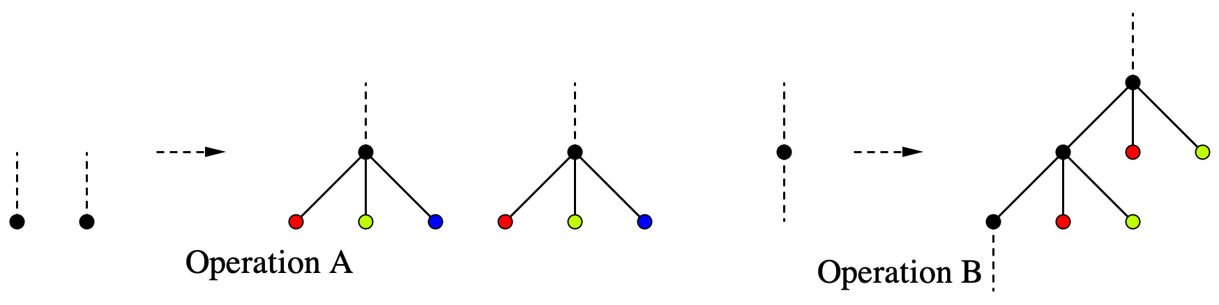
For any couple we can define two operations: operation where a leaf pair is replaced by a -mini couple, and operation where a node is replaced by a mini tree, see Figure 10. Then, we define a couple to be regular if it can be formed, starting from the trivial couple , by operations and . We also define a saturated paired tree to be a regular tree, if forms a regular couple with the trivial tree . Clearly the order of any regular couple and regular tree must be even.

Proposition 4.9.
For any couple there is a unique couple , which is prime in the sense that it does not contain any -mini couple or mini tree, such that is constructed from in a unique way, by replacing each leaf pair with a regular couple, and each branching node with a regular tree. This is called the skeleton of ; see Figure 11 for an illustration. The molecule does not contain a triple bond, and is regular if and only if is trivial. Moreover, the number of couples with order and fixed skeleton is at most .
More generally, let be any couple (not necessarily prime), one may form a couple by replacing each leaf pair with a regular couple and each branching node with a regular tree . We shall denote the the collection of all these and by , and write . Define to be the total order of regular couples and regular trees ; we may use etc. to denote suitable sub-collections if , and etc. are defined similarly.

Proof.
See Proposition 4.14 and Remark 4.15 of [14]. The molecule does not have triple bond, because is a prime couple. ∎
4.3. Blocks
We next define the notion of blocks (and hyper-blocks), which is an important class of atomic groups that occur in our proof.
Definition 4.10 (Blocks).
Given a molecule , an atomic group is called a block, if all atoms in have degree within , except for exactly two atoms and (called joints of the block), each of which having out-degree and in-degree (hence total degree ) within , see Figure 12. Define as the number of bonds between and . Note that , and if and only if is a double bond. Moreover, we define a hyper-block to be the atomic group formed by adding one bond between the two joints and of a block (we shall call this the adjoint of ), and define .
If two blocks share one common joint and no other common atom, then their union (or concatenation) is either a block or a hyper-block (depending on whether the two other joints of the two blocks are connected by a bond), see Figure 13. Note that a hyper-block cannot be concatenated with another block or hyper-block in this way. In general any finitely many (at least two) blocks can be concatenated to form a new block , or a new hyper-block , in which case we must have and .


Lemma 4.11.
Let be a molecule. Suppose , each of them is a block or a hyper-block, and , and .
Let and be the joints of , and and be the joints of . Suppose further that (i) is connected, and (ii) for any , the subset is either connected, or has two connected components containing and respectively, and (iii) the same holds for .
Then and are both blocks, and exactly one of the three following scenarios happens: (a) and share two common joints and no other common atom, and , (b) and share one common joint and no other common atom, and can be concatenated like in Definition 4.10; (c) is formed by concatenating two blocks and , and is formed by concatenating with another block (where ).
Proof.
(1) Suppose and share two common joints, say and . If a third atom , since , there must exist another atom . Since is connected by assumption (i), we can find a path from to that remains in but does not include either or . However we have and , so any path from to must include either or , contradiction. This tells us that . In this case there must be one (and exactly one) bond between and , so and we are in scenario (a). In fact, if , then has two bonds connecting to atoms in and two other bonds connecting to atoms in , and same for . Therefore every atom in will have degree (including and ), which contradicts the definition of molecule. The other cases are treated similarly.
(2) Suppose and share no common joint. Choose and , the same argument in (1) implies that either or must be an interior (i.e. non-joint) atom of . Similarly, either or must be an interior atom of . However, these four atoms cannot be all interior atoms because otherwise every atom in will again have degree . By symmetry, we may assume that is an interior atom of , is an interior atom of , and .
Now consider the atomic group , which is the disjoint union of and . If two atoms and from these two subsets are connected by a path in , then we again have a contradiction because this path cannot include either or . Using also assumption (ii), we know that and are two connected components of , and . It is now easy to see that and are two blocks that are concatenated at the common joint to form . Now by switching and and arguing similarly, we can see that is also a block, and is concatenated with at the common joint to form . Therefore, we are in scenario (c).
(3) Finally, suppose and share only one common joint, say . If , then clearly we are in scenario (b). If not, then there is a second atom . By repeating the arguments in (1) and (2), we know that is an interior atom of and is an interior atom of . Then all atoms in except will have degree , thus can only have degree (in-degree and out-degree , as total in-degree must equal total out-degree), which means that has two bonds connecting to atoms in . Now we can apply the same argument in (2) and conclude that and are two connected components of , and . But we already know is an interior atom of , which is impossible. This contradiction completes the proof. ∎
4.3.1. Blocks in a couple
We now discuss the relative position of a block in a couple .
Proposition 4.12.
Let be a couple and be a block with two joints and , and let .
- (1)
Then (up to symmetry) exactly one of the following two scenarios happens.
- •
(CL) or “cancellation” blocks: There is a child of and two children of , such that (i) has the same sign as , has sign and has sign , (ii) is a descendant but not of , and (iii) all the leaves in the set are completely paired, where denotes all nodes that are descendants of but not of or (in particular and ). See Figure 14.
- •
(CN) or “connectivity” blocks: There is a child of and of , such that (i) has the same sign as and has the same sign as , (ii) is either a descendant of or not a descendant of (similar for ), and (iii) all the leaves in the set are completely paired, where denotes all the nodes that are descendants of but not of , and all the nodes that are descendants of but not of (in particular and ). See Figure 15.
- •
- (2)
For (CL) blocks we can define a new couple by removing all nodes , and turning and into the three new children of with corresponding subtrees attached; here the position of as a child of remains the same as in , and the positions of and as children of are determined by their signs. Then, the molecule is formed from by merging all the atoms in (including two joints) into one single atom. We call this operation going from to splicing.
- (3)
For (CN) blocks, if we remove from any set of disjoint (CN) blocks in , where by removing a block we mean removing all bonds , then the resulting molecule is still connected (though it no longer comes from a couple). This remains true if we remove also a (CL) block, provided that both joints of this (CL) block have degree . Note that there is at most one such block due to Proposition 4.4; for simplicity we will call it a root block.

, and all the leaves in the red circle are completely paired.

Proof.
For any , there is a unique bond such that ; let be the other endpoint of , then is just the parent of in . Consider the path , then it either stays in or reaches the joints or at some point, due to the structure of . However, if it stays in then eventually it will reach one of the roots of , which is impossible because the roots have degree as atoms. Therefore it must reach or , which means that for any atom , must be a descendant of either or .
Now consider , there are two possibilities: (a) there is an atom such that is the parent of (as explained above), or (b) there is no such atom . For there are similarly these two possibilities. If case (a) holds for then by the same proof above, we know that is a descendant of ; since and cannot be a descendant of each other, by symmetry we have only two cases: either (a) holds for and (b) holds for , or (b) holds for both and . Below we define and as the two bonds connecting to atoms in , and similarly define and corresponding to .
(1) Suppose (a) holds for and (b) holds for . In particular is a descendant of , and are two children of ; let be the other child of . Similarly, are and one child of , let and be the two other children of . Clearly must have the same sign as and must have opposite sign with , because and have opposite directions, and the same for and . We will assume has sign and has sign .
Now we claim that if and only if . In fact, if then first is a descendant of as shown above; second, consider the path , then the node immediately before must be for some and thus cannot be by definition, hence is not a descendant of ; third, if the above path contains , then the node immediately before must be for some and thus cannot be or by definition, hence is not a descendant of or either.
Conversely, if is a descendant of but not of or , then the path must end at , and the node immediately before must not be . Thus this node must be for some , and the atoms involved in this path must all be in unless this path contains . But if belongs to this path, then the node immediately before it must not be or , so it must also be for some , and again all the atoms involved in this path must be in . In any case we have , so our claim is true.
Now with the above claim, it is easy to see that all the leaves in must be completely paired, and these leaf pairs exactly correspond to all LP bonds in . It is also clear that, merging to a single atom corresponds to removing all nodes , and the resulting molecule is exactly for the resulting couple .
(2) Suppose (b) holds for both and . In particular are two children of , let the other child of be . Similarly define , then must have the same sign as and has the same sign as , again due to the directions of the bonds . Moreover, if is a descendant of , then in the path , the second node does not belong to , and neither does any subsequent terms; thus the node immediately before cannot be for any , so it must be , which means that is a descendant of (actually also cannot equal because otherwise we would have an extra bond between and , turning into a hyper-block). Now, by arguing similarly as in (1) we can show that if and only if . This easily implies that all the leaves in are completely paired.
Next we prove the preservation of connectivity after removing any set of disjoint type (CN) blocks. In fact, we may define the molecule for generalized couples formed by two arbitrary trees which are not necessarily ternary trees (plus that we only keep the pairing structure but ignore the signs of nodes and directions of bonds), similar to Definition 4.2.
In this regard, removing a type (CN) block amounts to removing all nodes . What remains is a generalized couple formed by two trees in which is the only child of and is the only child of (the fact that and each has only one child in the new generalized couple, corresponds to the fact that and each has degree in the new molecule). This can be extended to the removal of multiple disjoint type (CN) blocks, and the resulting molecule is where is a generalized couple formed by two trees such that each branching node has either or children. However, the corresponding molecule is still connected, because each node can be connected to the root of its tree by using PC bonds, and there exists at least one LP bond between the two trees since the number of leaves in each tree is odd. This completes the proof.
Finally, let be a root (CL) block, i.e. both joints of has degree . Then, in the notation of Proposition 4.12, we must have (up to symmetry) that is the root of one tree in , and a child of (say ) is paired with the root of the other tree as leaves. Thus we have a couple rooted at and , and removing reduces to a molecule which equals plus two extra single bonds. Clearly is connected, as is the result of removing from it any number of (CN) blocks in . This completes the proof. ∎
Corollary 4.13.
Let be a couple and be a block or hyper-block that is concatenated by at least two blocks as in Definition 4.10, where . Then at most one can be a (CN) block. If is a block and all are (CL) blocks, then is a (CL) block. If is a block and there is one (CN) block , then after doing splicing at all other (CL) blocks, this becomes a single (CN) block .
Proof.
Let the joints of be and for . Recall the possibilities (a) and (b) defined in the proof of Proposition 4.12, which are stated for any joint of any block . If some is a (CN) block, then as in the proof of Proposition 4.12, (b) must happen for both joints and relative to the block . Thus (a) must happen for the joint relative to , and is a (CL) block. Moreover, (b) must happen for relative to , and hence (a) must happen for relative to , and so on. Of course we can also start with and proceed with etc., and altogether we know that all blocks other than must be (CL) blocks. If is a block, then after we splice at all the other (CL) blocks, this should remain unperturbed, as a (CN) block.
If is a block and all are (CL) blocks, then for each block , (a) must happen at one of its joints, say (if it is then the proof is the same by going in the other direction). Then (b) must happen for the joint relative to , and (a) must happen for relative to and so on. In the end (a) must happen for relative to (and hence relative to ), so is a (CL) block. ∎
5. Vines and twists
5.1. Vines
We are now ready to introduce the notion of vines which are the special kind of blocks that are of fundamental importance in our proof.
Definition 5.1 (Vines).
Vines55 5 The nomenclature comes from the shapes of the blocks drawn in Figure 16. are defined as the blocks (I)–(VIII) drawn in Figure 16. We also define the notion of ladders as drawn in Figure 16. For each ladder we also require that each pair of two parallel single bonds must have opposite directions, and define its length to be the number of double bonds in it minus one. We refer to vines (I)–(II) as bad vines, vines (III)–(VIII) as normal vines. Note that for all vines except vines (V) and vines (I) (see Definition 4.10), for which and respectively.
Define hyper-vines (or HV for short) to be the hyper-blocks that are adjoints of vines, as in Definition 4.10. We also define vine-chains (or VC), resp. hyper-vine-chains (or HVC), to be the blocks, resp. hyper-blocks, that are formed by concatenating finitely many vines as in Definition 4.10 (these vines are called ingredients). Note that a single vine is viewed as a VC, but an HV is not viewed as an HVC. It is easy to verify that assumptions (i) and (ii) in Lemma 4.11 hold for any HV, VC or HVC. For simplicity, we will refer to any HV, VC or HVC as vine-like objects.
Note that, if the molecule comes from a couple, then any vine could be a (CL) or (CN) vine depending on whether it is a (CL) or (CN) block.

Remark 5.2.
We make a few remarks about the illustrations in Figure 16:
- (1)
In each vine, the two joints are colored blue; the bonds at the joints are drawn with directions, indicating that the two bonds at each joint must have opposite directions.
- (2)
The other bonds are drawn without directions, meaning they are arbitrary, as long as requirements of a molecule are met (each non-joint atom has in-degree and out-degree ).
- (3)
In each vine, we may insert a ladder between each pair of parallel bonds that are drawn as dashed lines (distinguished by different colors).
- (4)
In the ladder, some bonds are drawn with directions, indicating that each pair of two parallel single bonds must have opposite directions.
5.1.1. Bad (CL) vines in a couple
We need to study the relative position of (CL) vines (I), and the part of (CL) vines (II) near one of its joints, in a couple.
Proposition 5.3.
Consider a (CL) vine with joints and . Let , by Proposition 4.12 we may assume is a descendant of , and also specify two children and of that have signs and respectively; let be the other child of , note that has the same sign as .
- (1)
If is vine (II), then is connected to two atoms and by single bonds, while and are connected by a double bond. Let , then (up to symmetry) exactly one of the following five scenarios happens. See Figure 17.
- (a)
Vine (II-a): is a child of , and is paired with one child of as leaves, and the other two children of are paired with the other two children of as leaves. Here neither nor is a descendant of the other, but they have a common ancestor, namely .
- (b)
Vine (II-b): is a child of , and is paired with one child of as leaves, and the other two children of are paired with the other two children of as leaves. Here neither nor is a descendant of the other, but they have a common ancestor, namely .
- (c)
Vine (II-c): is a child of and is a child of . One of the the other two children of is paired with one of the other children of as leaves, and the remaining child of is paired with as leaves. Here is a descendant of .
- (d)
Vine (II-d): and are two children of , and is paired with one child of as leaves, and the remaining child of is paired with another child of as leaves. Here is a descendant of .
- (e)
Vine (II-e): is a child of , and . The other two children of are paired with two of the children of as leaves. Here is a descendant of .
- (a)
- (2)
If is vine (I), then exactly one of the following two scenarios happens. See Figure 17.
- (a)
Vine (I-a): is the left or right child of , and is paired to the middle child of as leaves.
- (b)
Vine (I-b): is the middle of , and is paired to the left or right child of as leaves.
- (a)

For simplicity, below we will call a (CL) vine core if it is bad and not vine (II-e), and non-core if it is normal or vine (II-e).
Proof.
We examine the labels of each bond between using Definition 4.2. Note that, since is a (CL) vine, one of the bonds connecting to and must be labeled PC with labeled by C; moreover, some configurations are not possible (for example, the two bonds between and cannot both be labeled PC) due to basic properties of the couple (for example two branching nodes cannot be the parent of each other). By a simple enumeration and symmetry, we find that there is only one case for vine (I) and five cases for vine (II), as drawn in Figure 17.
For each case of labels, one can apply the definition of the label to deduce that the relation between has to be as in the corresponding figures. For example, for vine (II-a), by the PC bond between and , we know that must be a child of . By the two LP bonds between and , we know that the two other children of must be paired with two children of as leaves. By the LP bond between and , we know that the remaining child of must be paired to a child of as leaves, and this child of must be , which is drawn in blue. Clearly neither nor can be descendant of the other, but the have a common ancestor , so we arrive at the illustration of Vine (II-a) in Figure 17. The other cases are treated similarly. ∎
Remark 5.4.
We make a few remarks about the illustrations in Figure 17.
- (1)
- (2)
- (3)
The nodes represented by hollow dots instead of solid dots are called free children. These include and (except vine (II-e)), and either a child of for vines (II-c) and (II-d), or a child of for vines (I-a) and (I-b).
- (4)
- (5)
Note that the distinction between vines (I)–(VIII) only involves the structure of the molecule (as a directed graph), but the distinction between (CL) and (CN) vines, as well as families (II-a)–(II-e) etc., is intrinsic to the structure of the couple ; for instance, it does not make sense to talk about (CL) vines or vines (II-e) if does not have the form .
5.2. Twists
By exploiting the structure of bad (CL) vines in a couple, as described in Proposition 5.3, we can define the operation of twisting, which captures the cancellation between such vines.
Definition 5.5 (Twists).
Let be a given couple with the corresponding molecule .
- (1)
Given a core (CL) vine as in Proposition 5.3, let and for be as in that proposition. Then, we shall define a new couple , which we call a unit twist of , as follows.
First, in , let any possible parent-child relation, as well as any possible children pairings, between and , be exactly the same as in . Next, let the structure of excluding the subtrees rooted at and (or for vine (I)), be exactly the same as . Moreover, consider the free children in Figure 17 (as in Remark 5.4); we require that the positions of the two free children and (as children of ), as well as the positions of the two subtrees (namely and ) rooted at them, be switched66 6 They are switched because the sign of is changed (see Remark 5.7); if we locate as the child of other than that has sign (and same for ), then this remains the same for both couples. in compared to . For the other free child (if it exists), we require that its position (as a child of or ) and the subtree (namely ) rooted at it, be exactly the same in as in . Then, it is easy to see that there are exactly two options to insert , one as a child of , and the other as a child of (for vine (I), the two options are children of that has the same or opposite sign with ). One of these two choices leads to , and we define the couple given by the other choice as . Clearly is prime iff is.
- (2)
In the same way, start with a collection of (CL) vines , such that any two are either disjoint or only share one common joint and no other common atom (i.e. the union of all equals the disjoint union of some VC and HVC). Then, we call any block a twist of , if can be obtained from by performing the unit twist operation at a subset of these blocks, which only contains core vines. In particular, for any given and , the number of possible twists is a power of two, and at most .
Since the notion of twisting is of vital importance in our proof (especially in Section 8), we will make several remarks below explaining Definition 5.5 in more detail.
Remark 5.6.
We discuss an example of the (unit) twist operation in Definition 5.5. Suppose is vine (II-c) or (II-d) in Figure 17. Then we have that:
- (1)
The node is the left child of , and the middle child of is paired with the right child of as leaves.
- (2)
The left child of is a free child with subtree . The left and middle children of are the two free children and (or and ), with the subtrees rooted at and being and respectively.
- (3)
is a child of (or ), and the right child of is paired to a child of (or ) as leaves.
Now by Definition 5.5, all these properties must hold in both and ; also the structure of and , excluding the subtree rooted at , must be the same. This leaves only two possibilities: either is the middle child of and is paired to the right child of as leaves, or is the right child of and is paired to the middle child of as leaves. These are exactly vines (II-c) and (II-d) in in Proposition 5.3. Note that for vines (II-c) is the left child of and is the middle child, while for vines (II-d) is the left child and is the middle child, which is consistent with the description in Definition 5.5.
In the same way, we can see that performing one unit twist operation exactly switches vines (I-a), (II-a), (II-c) vines with vines (I-b), (II-b), (II-d) vines, respectively.
Remark 5.7.
Throughout the proof below, for any fixed (CL) vine , we always adopt the notations as in Proposition 4.12; for bad (CL) vines we also adopt the notations as in Proposition 5.3, whenever applicable. The following useful facts are easily verified from Definition 5.5. They are stated for unit twists but can be extended to general twists.
- (1)
Let and be unit twists of each other at a bad (CL) vine , then and are the same as directed graphs. They also have the same labelings of bonds, except at the atom (see Figure 17).
- (2)
Continuing (a), the only difference at is that the labels of the two bonds connecting to atoms in are switched (one label is PC with labeled C and the other label is LP).
- (3)
Moreover, if we do splicing (as defined in Proposition 4.12) for and the (CL) vine , or for and the same (CL) vine (as shown in (a) above), then the two resulting couples, defined as and , are exactly the same.
- (4)
Finally, the values of for any branching node are the same for and , while the values of are the opposite for and .

Remark 5.8.
We make another simple observation regarding decorations of couples and their twists. Let be a couple and be formed from by a unit twist (this is readily generalized to arbitrary twists). Then, the -decorations of are in one-to-one correspondence with -decorations of , where the values of for any branching node or leaf are the same in both cases, but one switches the values of and in both cases, see Figure 18.
Let be the couple formed from (or ) by doing splicing, then for any -decoration of and the corresponding -decoration of defined above, the decorations of inherited from them are the same; here inheriting means that the value of is kept the same for any , whether it is viewed as a node of or . This notion also applies to any subset of couples or molecules, or when a couple or molecule is reduced by repeated splicing (or merging) of vines, and will be used frequently below.
Definition 5.9.
Note that the unit twist operation in Definition 5.5 only changes the structure of the set defined in Proposition 4.12 (which is part of a ternary tree, obtained by taking the subtree rooted at and removing the subtrees rooted at , and ), and does not affect the rest of the couple , so we can view it as a unit twist for .
We may define another operation on which we call flipping, where we flip the signs of (and ), and switch the two subtrees rooted at the two other children nodes of , together with leaf pairings, see Figure 19. Note that unit twisting is an operation on , defined only for core (CL) vines (Proposition 5.3), that can be canonically extended to the couple. Flipping, however, is an operation on , defined for all (CL) vines , that in general cannot be canonically extended to the couple. However, if is concatenated with another (CL) vine above it, then flipping at can be extended to a couple operation, which is unit twisting at the vine .

Now, given a (CL) vine , there are possible structures for , where is the number of branching nodes in . We define two of them to be equivalent, if one can be formed from the other by flipping, and (if is a core (CL) vine) unit twisting. We call each equivalence class a code, denoted by . Note that for a core (CL) vine , each code contains exactly four elements, as shown in Figure 19; they are uniquely determined by the signs and . For other (CL) vines , each code contains exactly two elements; they are uniquely determined by , and the value of is determined by the code.
Let be a couple with a core (CL) vine , then by Definition 5.5 and the above discussions, we know that is in one-to-one correspondence with the quadruple , where and are as above, and is the branching node in that corresponds to the node of in (note that is determined by and ). We shall write this as , and note that making a unit twist for corresponds to changing the value of only. If is non-core then is still uniquely determined by the above quadruple, except that is now determined by .
5.3. Full twists
Finally, we extend the notion of twists to general couples by adding back the regular couples and regular trees in Proposition 4.9.
Definition 5.10 (Full twists).
Let be a couple, be its skeleton, and write as in Proposition 4.9.
- (1)
Fix one core (CL) vine . Now consider another couple , such that either equals , or is a unit twist of it as in Definition 5.5. In the unit twist case, consider the branching node (in the notation of Proposition 5.3), which occurs in both and . Consider also the leaf pair involving the non-free child of , which again occurs in both and , see Figure 17. Apart from these, any other branching node and leaf pair is exactly the same in the two couples and .
Now, if is a unit twist of , we say is a full unit twist of , if (i) for any branching node (or any leaf pair ), the regular trees and (or the regular couples and ) are the same, and (ii) the regular trees and , and the regular couples and , satisfy that . If , the definition is modified in the obvious way.
- (2)
In general, for any set of (CL) vines as in Definition 5.5, such that any two are either disjoint or only share one common joint and no other common atom, we define to be a full twist of , if can be constructed from by performing some full unit twist at each that is core.
Remark 5.11.
Let be a couple and be a collection of regular couples and regular trees as in Proposition 4.9. Suppose is a (CL) vine, let be the result of splicing at , then we have , with notations as in Definition 5.9. Therefore, we also have the one-to-one correspondence , where is the sub-collection of that involves and at nodes , and is the corresponding collection for , which is the same as the sub-collection that involves and at nodes .
If is a couple with skeleton , the we have by Proposition 4.9, and is also in one-to-one correspondence with the sextuple as above. If runs over all full unit twists of a given couple at a core (CL) vine , then only and in this sextuple may vary; in fact takes values in , while runs over the collections of and for , such that and are fixed when and , and that takes a fixed value.
6. estimates for regular couples and regular trees
6.1. Asymptotics and cancellations for
In this subsection we study expressions associated with regular couples (as well as similar expressions for regular trees). The main results are stated as follows.
Proposition 6.1.
Let be a regular couple of order , and be defined as in (2.14). Then, extends as a smooth function in and admits the decomposition , where the remainder satisfies the bound
| (6.1) |
where is defined as in (2.8). The main term equals the sum of at most terms of form
| (6.2) |
where each of these terms satisfies the estimate
| (6.3) |
In particular we also have
| (6.4) |
Now let be a regular tree of order . For , define in the same way as (2.14) but with a few differences: the -decoration is replaced by , the product is only taken over leaves of sign different from the lone leaf, and the domain is replaced by
| (6.5) |
where is the parent node of the lone leaf . Then we have the decomposition , and the main term equals the sum of at most terms of form
| (6.6) |
The bounds satisfied by , , and are the same as in (6.1), (6.3) and (6.4) above, except that the norm is replaced by , and the factor on the right hand side of (6.3) is replaced by . Finally, we have the simple identities (also for the variants)
| (6.7) |
Proposition 6.2.
6.2. Proof of Propositions 6.1 and 6.3
In this subsection we will prove Propositions 6.1 and 6.3. Note that Proposition 6.2 follows from the exact same calculations in Subsection 7.4 of [14], so we don’t repeat it here.
6.2.1. Proof of Proposition 6.1
First, (6.7) is obvious by definition in (2.14). The proof of other results goes along the same lines as the parallel results in [14] (Propositions 6.7, 7.4–7.7). In fact, the only difference between the results here and in [14] is an improved bound for the remainder in (6.1), as well as the bound for an improved norm in (6.3) compared to the estimate on the norm in [14] (the results for are similar). We shall explain below how these estimates follow by combining the analysis in [14] with new estimates improving Section 6 of [14]. We remark that the analysis in Sections 5 and 7 of [14] is independent of the chosen scaling law, and as such carries over to the current setting. The analysis in Section 6 of [14] is dependent on the scaling law, and we will provide the corresponding alternative bounds here, which carries over to the full range of scaling laws and provides the improved estimate on the remainder.
As such, we only need to prove (6.1) and the first part of (6.3). The latter follows from the fact that is zero unless is a dominant couple (cf. Proposition 7.4 of [14]), and in which case is an explicit homogeneous polynomial in the variables and . The desired bound then follows. We now focus on the remainder estimate in (6.1).
We start by recalling some notation for regular couples: From equation (2.14), we may write
where
| (6.10) |
Here, is defined in (2.15). Given a regular couple , a natural pairing exists between the branching nodes in (cf. Proposition 4.3 and 4.8 in [14]). We shall fix a choice of (here for “choice”), which contains exactly one branching node in each pair. As such, for any decoration of , we must have for any pair of branching nodes. This allows us to define by
| (6.11) |
assuming that is defined such that for each pair .
Now Proposition 5.1 of [14] shows that, if is a regular couple of order , then the function is the sum of at most terms. For each term there exists a subset , such that this term has form
| (6.12) |
for , where is as in Section 2.2. In (6.12) the function satisfies the estimate
| (6.13) |
for any multi-index , as well as
| (6.14) |
We will denote the integral in (6.12) by , so we have
| (6.15) |
We should remark here that the powers on the weights and are stated differently in Proposition 5.1 of [14], but a careful inspection of the proof in Section 5 of [14] shows that the bounds in (6.13) and (6.14) actually hold as well. In fact, this relies on the fact that the corresponding integrals appearing in the proof of Proposition 5.1 of [14] have a form like
which are bounded for all ; here and is one of the denominators ( or in the first expression, and or or in the second).
As a consequence, we can write
| (6.16) |
The remainder appears upon approximating the sum in with an integral. This approximation, along with the estimates on the remainder , is done in Section 6 of [14] (See Propositions 6.1 and 6.7). It is here that the argument becomes dependent on the chosen scaling law. Indeed, we will provide below the alternative propositions that will allow to prove the claimed bound for in (6.1).
Proposition 6.4.
Consider the following expression
| (6.17) |
where . Assume there is a (strict) partial ordering on , and that the followings hold for the functions and :
(1) The function satisfies the bound (here denotes the Fourier transform in )
| (6.18) |
(2) This is supported in the set
| (6.19) |
where are constants, and are constant vectors. Each is a linear function that equals either , or or for some , similarly each equals either , or or for some .
(3) For some set , the function has the expression
| (6.20) |
where is as in Section 2.2, and for any we have
| (6.21) |
Assume . Then we have
| (6.22) |
Moreover, defining
| (6.23) |
where the singularities are treated using the Cauchy principal value, we have
| (6.24) |
We shall prove this proposition by relying on a series of Lemmas formulated and proved below. In what follows, we assume that and use the notation . The first lemma replaces Lemma 6.2 of [14].
Lemma 6.5.
Suppose is a function satisfying the bounds
| (6.25) |
for all multi-indices . Then we have:
(1) The following bound
| (6.26) |
holds uniformly in .
(2) Suppose, in addition, that is supported on the set . Then, there holds
| (6.27) |
uniformly in . In particular, we have
| (6.28) |
uniformly in .
Proof.
With no loss of generality we assume . Part (1) follows easily by translating in and , and then applying the stationary phase lemma to estimate the integral by . To prove part (2), we define , and split the left-hand side of (6.27) into two parts and defined as follows:
Part A: where or . For this part, we will fix the variables and integrate by parts in as follows: Defining , , , and , then up to a unimodular constant independent of the variables, we can write the integral in as
Integrating by parts many times, using the last oscillatory factor and the fact that that either or , we obtain that the contribution of Part A is better than acceptable.
Part B: where and . Recall that since and , we have that , and hence for fixed the number of choices of in the sum in this part B is . We further split this part into two: Part B1 in which the integral is over and part B2 for which . For B2, we simply use stationary phase again in the integral to estimate it by , so the contribution of this part is bounded by
Moving back to , we notice that in this case , which implies that, for each fixed , there is at most one element in the whole sum over . Now we split the integral into dyadic pieces, and rewrite the contribution of B1 as
Let . For the part of the dyadic sum with , notice that since and , we must have that . Therefore, if we just use stationary phase again in the integral, we can estimate the sum over by
as needed. This leaves us with the sum over . Assume with no loss of generality that . Since , we have that where denotes the fractional part. Since we also have that belongs to an interval of size , it follows that belongs to a set of measure . Hence, belongs to a set of measure . As a result, recall that for fixed the the sum over has at most one element and the integral in is by stationary phase, we can estimate
which sums in to give,
This finishes the proof. ∎
The following lemma replaces Lemma 6.4 of [14].
Lemma 6.6.
Suppose that is a function satisfying (6.25).
(1) If is supported on , then the following bound holds uniformly in :
| (6.29) |
(2) If is supported on the set , then the following improved estimate holds uniformly in : for ,
| (6.30) |
Proof.
Part (1) is implied by Lemma 6.4 of [14] (which even extends to supported on . So we focus on part (2); if then (6.30) is trivial due to the factor , so we will assume . Recall that, where . We make the change of variables
The sum in then becomes the linear combination of four sums, which are taken over , or , or , or . We will only consider the first sum, and it will be obvious from the proof that the other sums are estimated similarly. Define
which has all derivatives in up to order uniformly bounded, and is supported in the set , where are determined by .
Now, by possibly redefining , we need to show that the function
satisfies the bounds in (6.30) when is supported on , noting that in the above sum we must have and . Now, recall the Gauss sums and defined by
| (6.31) |
where is the floor function, and notice that since , we can write
where etc., and is obtained from by taking one derivative in each of the variables (and hence has the same support properties). By rescaling in , we obtain that
where is a set in of volume . We will be done then once we show that, uniformly in , there holds
First note that using the trivial bound , and by our choice of , it is enough to show that
which is implied by proving that, uniformly in satisfying , there holds
| (6.32) |
For this, let be the interval of integration above, and let us assume that for some dyadic integer . We will rely on the Gauss lemma for Gauss sums in (6.31) which gives that if for some with , then
Here we recall that can be approximated by such rational number in the above fashion by Dirichlet’s Approximation Theorem. Let us assume that for some dyadic integer with and that with (with the obvious modification for ), so that
First note that if , then on , which gives a bound that is much better than (6.32). Otherwise, we have on . Also, note that since on , we must have that for any with , as well as . As a result, we obtain that
which gives the result since . ∎
Lemma 6.7.
Suppose satisfyies (6.25) without . Let and .
(1) Suppose is a function such that , then
| (6.33) |
uniformly in . The same holds if is replaced by where satisfies for all multi-indices .
(2) Suppose further that , then
| (6.34) | ||||
uniformly in .
Proof.
The proof is the same as that of Lemma 6.5 of [14] (with the weight in (2) replaced by which does not affect the proof). We omit the details. ∎
Proof of Proposition 6.4.
With Proposition 6.4 in hand, we can apply it to the sum in (6.16) exactly as is done in the proof of Proposition 6.7 of [14]: First, for any we define and , so we have by (2.6). As explained in [14], the linear mapping
is volume preserving and preserves the lattice , where are the decorations of some leaf pairs (out of the pairs in total) in the -decoration . We can then rewrite the sum in (6.16) as
| (6.35) |
where (which depends only on ) and , with each and equaling plus some linear combination of .
The first thing to notice from (6.35) is that is clearly smooth in , as any derivative in falls on the function. This allows to write (6.35), as well as its derivatives in up to order , in the form (6.17) as explained in details in the proof of Proposition 6.7 of [14], which allows us to apply Proposition 6.4. Consequently, we obtain that if be a regular couple of order where , then we have , where
| (6.36) |
Here the error term satisfies (6.1) for each , by examining the gain of power in each error term occurring in Lemmas 6.5, 6.6, and 6.7, and noticing that . The exact expression , which is provided in Proposition 6.7 of [14], is not needed here, but we shall need some of its properties which are recalled below. We refer the reader to [14] for the complete details, which are the same in our case here. This finishes the proof of Proposition 6.1 (for couples, but the results for regular trees are proved similarly using the fact that a regular tree forms a regular couple with the trivial tree, see Proposition 6.10 of [14]).
6.2.2. Proof of Proposition 6.3
We start by recalling some facts concerning the structure of regular and dominant couples from Section 4 of [14]. A regular chain is a saturated paired tree, obtained by repeatedly applying operation (attaching one of the mini trees in Figure 20 at either a branching node or the lone leaf, as described in Definition 4.8), starting from the trivial tree . A regular double chain is a couple consisting of two regular chains (where, of course, the lone leaves of the two regular chains are paired). It can also be obtained by repeatedly applying operation at either a branching node or a lone leaf, starting from the trivial couple . The order of a regular chain is always an even number . The branching nodes are naturally ordered by parent-child relation; denote them by from top to bottom. A dominant chain is a special case of regular chain in which the application of operation is only done at the lone leaves. In this case, we can group the branching nodes from top to bottom as pairs , , which are exactly the branching nodes of the mini tree attached in the -th application of operation . Note that the signs of the nodes are all the same.
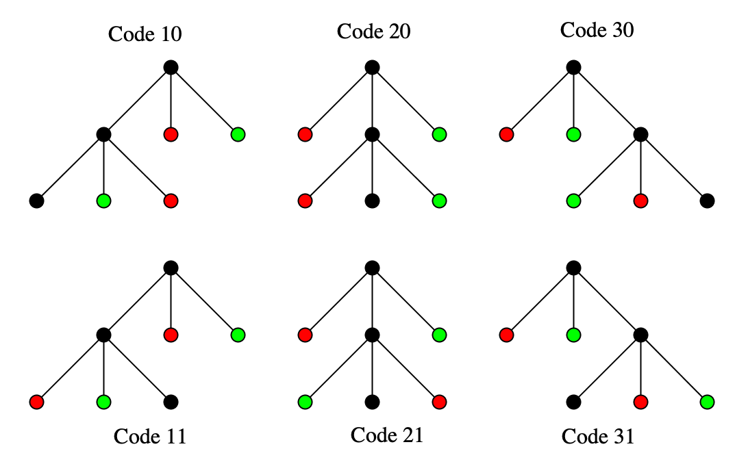
The structure theorem of regular couples states that, for any nontrivial regular couple , there exists a regular couple which is either a -mini couple or a regular double chain, such that is formed by replacing each leaf pair in with a regular couple (cf. Proposition 4.8 of [14]). In the first case, we call the couple type 1 and in the second we call it type 2. For type 2 regular couples , if we we require that the couple replacing the lone leaf pair of is trivial or has type 1, then this is unique (cf. Proposition 4.10 of [14]).
Dominant couples are a special class of regular couples defined inductively as follows. First the trivial couple is dominant. Suppose , let be uniquely determined as explained above, and let be the regular couples in replacing leaf pairs in . Then we define to be dominant, if (i) is either a -mini couple or a regular double chain formed by two dominant chains, and (ii) each regular couple is dominant. For a dominant couple of type 2, we enumerate the couples replacing leaf pairs as follows: is formed of two dominant chains and ; each of is formed by attaching mini trees (from root to lone-leaf) at the nodes (). Look at the -th mini tree in , we define the dominant couple replacing the pair of red leaves in Figure 20 by , and define the regular couple in replacing the pair of green leaves in Figure 20 by . Then, for the dominant couple , we have
| (6.37) |
and we define
| (6.38) |
Here in (6.37) and (6.38), the couples , where and , are the ones described above, and (and ) are defined correspondingly; similarly for , and . The notation for a dominant couple of type 1 is much simpler as we denote by the three couples replacing the three leaf pairs (from left to right) of a -mini couple. Here, we set where is the root with sign.
Motivated by (6.16) and still recalling [14], we define below the notion of special subsets of for a dominant couple . The pair will be called an enhanced dominant couple, on which which we also define an equivalence relation between two enhanced dominant couples and , as follows. First is a special subset and the enhanced trivial couple is only equivalent to itself.
Next, if is a dominant couple of type 1, then is special if and only if (i.e. is not in ) where is special. If we denote by the three enhanced dominant couples defining , and similarly for , we say if and only if for .
Now let and be as before, but suppose and have type . Let be associated with as explained above, and similarly for (same for the other objects appearing below). Suppose the two regular chains of have order and respectively, and let the branching nodes in be . In the construction of , at each node () one of the six mini trees (Figure 20) is attached, and is the other branching node of this mini tree. We define a set to be special if and only if
| (6.39) |
for some special subsets and , and some subsets . Similar representations are defined for . For and each , consider the tuple . Here if and otherwise, is the first digit of the code of the mini tree attached at the node . Moreover is the equivalence class of the enhanced dominant couple for , and let be the equivalence class of the enhanced dominant couple .
We now define , if and only if (i) , and (ii) the tuples coming from (there are total of them) form a permutation of the corresponding tuples coming from (there are total of them), and (iii) . Finally, note that if and are equivalent then and . When with , we also say that .
Similarly, we can define the notions of dominant trees , special subsets , enhanced dominant trees , and equivalence relations among them, similar to type 2 dominant couples above, except that there there is only one dominant chain, and so there is no lone pair couple . In particular, if we denote by the dominant chain of order such that is obtained by replacing leaf pairs of by dominant couples, then the equivalence class of the enhanced dominant tree is determined by specifying tuples exactly as defined above.
With this notation in hand, we can recount the main results in Section 7 of [14], which carry over verbatum to our setting here:
- •
- •
Let be a dominant couple. Then where the sum is over special subsets as defined above and is defined in (6.36). The function is independent of and may be denoted . Moreover, these functions satisfy some explicit recurrence relation, described as follows. First for the trivial couple (Proposition 7.5 of [14]). If has type , then it is formed from the -mini couple by replacing its three leaf pairs by dominant couples . In this case, we have
(6.40) In particular is a function of for type dominant couples . Finally, if has type , then is formed from a regular double chain , which consists of two dominant chains, by replacing each leaf pair in with a dominant couple. Using the notations described above for the structure of and in this case, we have
(6.41) Here we understand that and .
- •
- •
Similarly, for a dominant tree , and with the notation described above, we have
(6.42) and is real-valued and depends only on the equivalence class of the enhanced dominant tree .
We are now finally ready to give the proof of (6.9). In fact, we shall split this sum into subsets and show that the sum of each subset is real. To define these subsets, we first notice that
| (6.43) |
where the sum is now over enhanced dominant couples of order and enhanced dominant trees of order . Recall that each belongs to an equivalence class that is completely determined by specifying tuples () and an equivalence class for the enhanced dominant couple . Note that is of type 1 if and only if , in which case is the equivalence class of the enhanced dominant couple . Similarly, belongs to an equivalence class of enhanced dominant trees that is completely determined by specifying tuples .
Suppose we fix the value , fix a collection of tuples , and fix an equivalence class , and then sum in (6.43) only for that belong to equivalence classes formed from this collection. We will show that this sum is real valued, which then completes the proof. Denote by all possible (enhanced dominant) couple-tree pairs that belong to equivalence classes formed from this given collection. Note that for any , the total order , the sum of the cardinalities of the special subsets for and for , and the product are all the same. Moreover, the product is also the same for all enhanced dominant since it is a product of factors determined by the tuples and the equivalence class (see Proposition 7.9 of [14]). Hence, for some real-valued function we have
| (6.44) |
We will show that this quantity is real, by showing that the sum vanishes unless is empty, in which case reality follows from that the evident reality of and . To see this, let us assume that for (recall that this value is the same for all ), and consider the sum on the right hand side of (6.44). We first note that from Proposition 7.8 of [14], if is an equivalence class of enhanced dominant couples , with , then
| (6.45) |
As a result, by (6.40)–(6.42), the sum in (6.44) is a linear combination of factors of the form (possibly with different arguments/variables), hence it vanishes unless all the equivalence classes , and have empty special subsets (recall that is constant on an equivalence class). Moreover, since is constant over , we may replace the factors in (6.44) by and prove the vanishing of the resulting expression
| (6.46) |
If , then we have a decomposition where are the orders of three dominant chains associated to the dominant couple and dominant tree , as well as a division of the tuples into three groups: one with elements denoted by (), one with elements (, and one with elements (). Moreover, since are just the first digits of the codes of the mini trees appearing in the structure of and , the corresponding second digits can be arbitrary (and and do not depend on this second digit) which results in a factor. Putting together, if we sum over all possible —which means summing over all possible decompositions of and permutations of the tuples, and then summing over all possible and —we would get
| (6.47) | ||||
Here in (6.47) the sum is taken over all permutations of the tuples . Moreover and represent the first (“”) component of and , the function equals where represents the last two (“”) components of , and and are defined similarly. Arranging all the time variables in decreasing order, and renaming them as , we can write
where the first sum is over all permutations of the tuples , and the second sum is over all partitions of the set into three subsets , and is the first (“”) component of . Now, notice that
if , then at least one of the , so the above product vanishes and hence also vanishes. This finishes the proof.
6.3. Reduction to prime couples
Using Proposition 6.1, we can reduce the expression for any couple , defined in (2.14), to a similar expression associated with the skeleton of , in the same way as in Section 8.1 of [14].
Recall from (2.14) that
| (6.48) |
where is the order of , is the domain defined in (2.15), is a -decoration and other objects are defined as before, all associated to the couple . By repeating the arguments in Subsection 8.1 of [14], using also the notation in Proposition 4.9, we get
| (6.49) |
where is the order of , is the domain defined in (2.15) but with , and is a -decoration, the other objects are as before but associated to the couple . Here in (6.49), the first product is taken over all leaf pairs where has sign , the second product is taken over all branching nodes , and represents the parent of (if is the root of a tree then should be replaced by ).
7. estimates for vines
7.1. Two general estimates for sum-integrals
Before getting to the needed estimates for vines, we first state two general results about expressions that are sums of time-oscillatory integrals.
Lemma 7.1.
Fix . For , consider the output variables and , and parameters . Assume each of is restricted to a fixed unit ball, and and . Let the input variables be and ; denote .
Suppose there exist alternative variables and , where we write and , such that: (i) we have and for some matrices and some constant vectors depending only on , such that all coefficients of are integers ; (ii) for each there exists such that is an integer linear combination of and with absolute value sum , such that ; (iii) any component of the vector x (such as or ) is the sum or difference of two variables, each which is a component of the vector k or or . Now define
| (7.1) |
Here in (7.1), is the domain of defined by the following conditions: (i) for any , and ; (ii) any fixed collection of inequalities of form , , or . For each , we allow and to depend on the parameters and assume
| (7.2) |
Moreover for , and if , then should be replaced by one of . Finally, assume one of the followings:
- (1)
The conditions in the definition of includes either or ,
- (2)
The summand-integrand in contains an extra factor of , in addition to (7.1),
- (3)
The summand-integrand in contains an extra factor of .
- (4)
For at least one of the , one of the two bounds in (7.2) is replaced by
Then, uniformly in and in the choice of the unit balls containing described above, and with the norm taken in , we have that
| (7.3) |
Proof.
Step 1: Preparations. Using the decay of , we can localize into sets of the form , where and sum the obtained estimate in at the end. Once this set of is fixed, we notice that there is choices for the integer part of the coordinates of . Similarly, once we fix all those integer parts, there are choices for the integer part of the coordinates of , and so on. As a result, at the expense of a multiplicative factor of , we may fix points so that . Consequently, since each is the difference of some and , we may assume that for some fixed we have and (where and may depend on the unit balls containing ). Finally, if is fixed, we may express one of the (for example ) as an affine linear combination of the others. This allows us to define the change of variables which is affine and volume preserving, and preserves the lattice (at most up to an absolute constant).
Now set , which is a function that satisfies the same conditions (6.18) and (6.19) (with and ) of Proposition 6.4 in the variables . In fact, (6.18) holds if is regarded as a function of , and thus it also holds for due to the properties of the affine linear transform. As such, by expanding in terms of its Fourier transform, we can replace this function by , with one extra weight or if needed. We thus reduce to
| (7.4) | ||||
for some set depending on . Below we first study , which we will bound uniformly in all variables and parameters .
Step 2: Continuous approximation. We shall neglect all the exponential factors in outside the sums in in (7.4) and take absolute value outside this sum. This allows to enlarge the domain (but still keeping the restriction in (a) if applicable) and factorize the whole expression into a product of terms for . We will focus on the factor, as others are similar and easier. This factor then reads
where with the extra restriction or in (a) if applicable. We may change the variables where and split the integral into two regions: where and where . Denote the contributions of those two regions by and respectively.
As for , we do Poisson summation in the variables and obtain that , where
Here is a function satisfying (6.25) uniformly in . Note that is bounded using Lemma 6.5 by
where we integrate in trivially. Moreover, due to the proof of Lemma 6.5, the bound can be improved to , unless . In the latter case, since , we must have . Therefore we can gain the power using the or as above.
Now we are left with . By stationary phase, the integral in is bounded by , so trivially if without extra restrictions (this applies for example to for ). For we have one of the assumptions (a)–(c) available, which will lead to further power gains. In fact, since , case (b) already implies the gain which suffices for (7.3); for (c), the extra factor can be transformed to a gain of since is still integrable in . Finally, in case (a), we have that or , which means that . Thus, integrating in with fixed gives an extra factor of in estimating , which also gives the gain .
Summing up, in all cases we have proved that and for , which then implies uniformly in and .
Step 3: Going from to . Recall that is defined as in (7.4) and is function valued in a Banach space with . Now it suffices to prove that . Note that, if we insert suitable time cutoff functions to the definition of in (7.4), then a simple integration by parts with (7.4) gives
| (7.5) |
which immediately implies (7.3) if we restrict to .
Now if instead , then we may replace the norm by the norm, and then sum over (which has choices due to the support assumption). Then we are dealing with the expression (or ) with the values of fixed, so the value of is also fixed. Integrating by parts in in (7.5) again, we get
| (7.6) |
where . By (7.4), this is defined similar to , but without the and factors and with one of the or variables fixed. Going back to the argument in Step 2, we can then estimate at most one trivially (say ) while the other are still bounded as above, and gain a power from (7.6), which completes the proof. ∎
Lemma 7.2.
Fix and , consider the same setting as in Lemma 7.1, but with the following differences. First, there are three more vector variables which we call in addition to ; accordingly, there are three more time variables in addition to and three more parameters in addition to . There are also three more alternative variables in additional to and in addition to . Let the definitions of x, k and include these extra variables, then they satisfy the same assumptions as in Lemma 7.1.
Then is defined as in (7.1), but we also sum over the new variables and integrate over the new variables. The domain defined in the same way as in Lemma 7.1 (except we include the new variables). The summand-integrand in is the same as in (7.1), and the bounds in (7.2) are also the same, except that (i) we also include the new and variables and the corresponding and functions that also satisfy (7.2), and (ii) we also include the extra factors
where , and with . Finally, we do not require one of the scenarios (a)–(c) to happen as in Lemma 7.1.
Then, uniformly in and in the choice of the unit balls containing described above, and with the norm taken in , we have that
| (7.7) |
Proof.
We perform the same reduction procedure as in the proof of Lemma 7.1. By restricting each and to a unit ball, expanding (which is the product of all the and factors) using Fourier integral, writing as an integral of in , and enlarging the time integration domain, we can reduce to expressions, which we denote by and . In fact, the expressions are exactly the same as in the proof of Lemma 7.1, and satisfy the same bounds ; therefore it suffices to study , which has the expression
| (7.8) |
with fixed vectors . By integrating trivially in , defining for with fixed , and applying Poisson summation as in the proof of Lemma 7.1 above, we can reduce to
| (7.9) |
where . To control this last expression, note that due to the assumption . For fixed , the phase function
satisfies for some fixed (which may depend on ), therefore for all but values of , the integral in can be controlled trivially by integrating by parts. For these values of , a simple stationary phase argument yields that the integral in integral is bounded by , which is integrable in for . This implies that , and combining with the bounds for other implies that
Then, repeating the last part of the proof in Lemma 7.1 and noticing that we are allowed to lose here, we can easily deduce (7.7). ∎
Corollary 7.3.
Fix . Consider the following setting, which is basically a “concatenation” of Lemma 7.2: the output variables are denoted , with each in a unit fixed ball. The input variables are and where and (but excluding ), with . The parameters are as above. The alternative variables are and , and (including ) satisfy the same properties as in Lemma 7.2 and Lemma 7.1), with in assumption (ii) of Lemma 7.1. The expression is defined as in (7.1) with summation and integration in all input variables (vector and time, see above). The domain is defined in the same way but involves all the time variables, and the summand-integrand in includes the following factors:
- •
Functions and for that each satisfies (7.2);
- •
- •
Extra factors of for , where equals plus or minus a vector in , and is an arbitrary linear combination of the variables and .
Then, uniformly in parameters and in the choice of the unit balls containing described above, and with the norm taken in , we have that
| (7.10) |
Proof.
The proof is almost the same as Lemma 7.2. We write as an integral of in , and use the same arguments as in the proof of Lemma 7.1 and 7.2 to reduce the norm of to the norm of with loss. Then, in estimating we may make the same reductions, sum in variables an integrate in variables trivially, and then reduce to the same and quantities as occurred in the proof of Lemma 7.2. These quantities are then estimated in the same way, noticing that the linear phases do not affect any part of the proof. Putting together, and noticing that the summation in each variables leads to a factor of , this proves (7.10). ∎
7.2. Application to vines
Using Lemmas 7.1–7.2, Definition 5.10 and Remark 5.11, we can prove the estimates regarding the part of the expression in (6.49) where we only sum and integrate over the variables corresponding to a bad or normal vine in .
7.2.1. Estimates for vines
Given a couple (not necessarily prime) and a collection of regular trees and regular couples as in Proposition 4.9, let . Fix also a (CL) vine , then we can write by Remark 5.11. we shall fix and let and vary as in Remark 5.11; in particular is fixed as in the notion of Definition 5.9.
Define to be the number of branching nodes in , and . Consider the formula (6.49) but with replaced by (and associated notations changed accordingly, like replaced by etc.). For later purposes, we also fix a set containing , and a Banach space valued function . Define the expression similar to in (6.49), but that:
- (1)
We replace the power (where is the order of ) by ;
- (2)
We replace the factor by the product of where runs over all branching nodes in ;
- (3)
In the summation , we only sum over the variables for (including branching nodes and leaves), and treat the other variables as fixed. We also replace by the product of factors on the right hand side of (2.10), but only for . In particular, we have that .
- (4)
In the integral , we only integrate over the variables for all branching nodes , and treat the other variables as parameters.
- (5)
In the first product , we only include those factors where ; in the products and , we only include those factors where .
- (6)
We include the function as a factor in the summand-integrand, where in the place of we plug in if , and plug in otherwise.
Note that depends on and , and depends on only via . Its output variables are and time variables . Since , we may write this function as
| (7.11) |
where is replaced by if , and by otherwise.
Remark 7.4.
Suppose the function does not depend on . If we fix and flip (which corresponds to flipping ), then the function , written exactly as in (7.11), does not change. In fact, consider the decorations of and its flipping, see Figure 19, where the values of and are switched. If we write down the whole expression , which is (6.49) modified by (a)–(f) above, in these two cases, we can verify that they match exactly term by term, hence the results are the same.
Proposition 7.5.
Suppose is a bad (CL) vine. In the above setting, let and be fixed, then for we have
| (7.12) |
Here , and the summation in (7.12) is taken over all choices of as in Remark 5.11. More precisely, if is vine (II-e) then and are fixed; if is not vine (II-e) then and is such that and are fixed when and , and the value of is also fixed.
Proof.
The proof is elaborate due to the many cases and arguments involved, so we divide it into several steps. We assume throughout that .
Step 1: Reductions. By definition, for each fixed , the summand on the left hand side of (7.12) takes the form (we omit dependence on for convenience, same below)
| (7.13) |
Here, we define as the product of where runs over all branching nodes in ; similarly define and as in the definition of above (In particular ). Let and be the two children of other than , note that
since each factor with appears twice in the sum with opposite signs except for and . Thus, we can rewrite (7.13) as
| (7.14) |
Step 2: Parametrization for vines (II). We start by reparametrizing the expression of in (7.14). For this, we will need the information contained in Figures 14 and Figure 21 (A) for vine (II). From the latter figure, we denote by the atoms forming the vine with joints at , such that is connected by a double bond to . We denote by the corresponding branching nodes in the couple, which are the branching nodes of . Given a decoration for , we get a decoration of the bonds of the vine as explained in Definition 4.6. Note that there is a total of branching nodes in , and as a result a total of leaf pairs (recall that ). We will denote the decoration of leaf pairs by , and that of the branching nodes by . Those two sets decorate the bonds in vine as is shown in Figure 21 (A), where we denote by the decoration of double bonds between and , by that between and , and by that between and for (with and decorating the two bonds connecting and respectively, and similarly for and decorating the bonds connected to from and ). Finally, we also define if bond decorated by is outgoing from for or from for , and otherwise. Note that specifying completely specifies the directions of all the bonds in except for the horizontal double bonds in Figure 21 (A).

From this decoration of the bonds and using Definition 4.6, we have that
and we call this common value . Note that is fixed and is nonzero due to Section 7.2.1 (c). Moreover, we have from (4.4) that
| (7.15) |
As a result of this, we can define new variables () such that (a) we have which is specified as in part (f) of Section 7.2.1, (b) each of is the difference of two vectors among for , (c) for we have
where for some with , and (d) for we have that
where for some and with .
As a result of all this, we get a set of variables to replace the variables for (of which there are corresponding to leaf pairs , and another corresponding to branching nodes ). If we write , and , then we have that: (i) and for some matrices and some constant vectors depending only on , such that all coefficients of are integers ; (ii) for each component () of , there exists , where is a descendent of , such that is an integer linear combination of and with absolute value sum , such that ; (iii) any component of is the sum or difference of two variables, each of which is a component of either or . Here the proof of (i) and (iii) and obvious, and (ii) follows from Lemma 6.6 of [14].
With the above reparametrization, (7.14) can also be written as
| (7.16) | ||||
This expression will not be used in Step 3, but will be used in Step 4 below. Moreover, once we confirm , we will replace factor by , since corresponds to the case where some or equals or some other fixed constant, which means we can sum over them trivially, gain a power using , and treat the rest of the variables using the same arguments below.
Step 3: A counting argument. We now treat the case where is vine (II), and or . In this case we do not need the cancellation structure, and as such we shall estimate each by itself, and use that there or elements in the sum over .
Start with the expression of in (7.14). At this point, suppose we restrict each of to a unit ball as in the in (7.12). We may repeat the arguments in the proof of Lemma 7.1, using (i)–(iii) above, to also restrict and each , as well as for all nodes , to a unit ball; all these unit balls will be fixed throughout the rest of the proof. As such we may assume , and henceforth expand it as a Fourier integral, so that the function in (7.12) is replaced by the product
| (7.17) |
where is a bounded function. Note that by doing this we can also exploit the weights of form whenever needed. In the same way, we can expand all the and functions as time Fourier integrals to obtain a linear combination of functions
for different choices of , with the coefficient being a weighted integrable function with a suitable weight, and where is a bounded function of all the variables. Below we may fix one choice of ; by doing so we may also exploit the weight whenever needed. As a result of, we can write in (7.14) as a linear combination of
| (7.18) |
where for , and
where is a shift of by elements of , and we also allow a shift of by . Also, is a bounded function that is localized in a fixed unit size box for each of its variables. Fixing the integer parts of as (each of which having at most possibilities), by summing over all these integer parts, we can bound the Fourier transform of (7.18) by
| (7.19) |
where the sum satisfies the additional localization that for each . The result (7.12) will follow from the following two estimates:
| (7.20) | ||||
| (7.21) |
Those two estimates are enough to give (7.12), since shifts of , and can be absorbed by the weights and .
To prove (7.20), we note that for some function by changing time variables, and by Lemma A.6 (1) we can bound by
where is obtained from by an invertible (actually lower triangular) linear transformation with integer coefficients, and is the sum of at most two variables. Since each has at most choices, we can easily sum over all , equivalently all , and apply Lemma A.6 (2) to transform from to , and get (7.20).
To prove (7.21), we upper bound by 1 which reduces the sum into a counting problem for satisfying all the decoration and localization assumptions as before, and in addition the condition that for each belongs to an interval of length . By the reparametrization in Step 2 above, this is a equivalent to counting the number of choices for the variables , each restricted to a fixed unit ball, such that each of ) is restricted to an interval of length .
Now if , we can bound the number of choices of by using Lemma A.3 (1), and the number of choices for each by using Lemma A.2 (2). This implies (7.21), noticing that for vines (II). If and , then we can bound the number of choices of by using Lemma A.3 (1), and the number of choices for each by using Lemma A.2 (2), which again implies (7.21).
Step 4: The cancellation argument. We now treat the case where is vine (II), and . In this case we need to rely on the cancellation happening in the sum over of the terms defined in (7.16). For this cancellation to manifest itself, we need to utilize the couple structure near , which is depicted in Figure 17.
We start with the easiest case, which is that of vine (II-e). In this case, we will estimate each element of the sum over separately and use that there are elements in this sum. At this point we can repeat the arguments in Step 3 to localize each of the and variables to a fixed unit ball, and consequently expand into (7.17) and each and as time Fourier integrals, to reduce (7.16) to at most expressions of form
Here is a fixed vector, is a linear combination of and the Fourier variables occurring in the expansions of and as above, and is an expression in the form (7.1), which can be obtained after defining the new time variables , for , and . The domain of integration after the change of variables is the same as described in Lemma 7.1, with replaced by . Moreover, due to the structure of the couple in vine (II-e) (see Figure 17), namely the fact that is a parent of and child of , we have the additional condition (a) in Lemma 7.1. As a result, by (7.3), we have that
After summing over , applying Lemma A.6 (2), and including the factors and etc., this implies (7.12). Note that the shifts is again absorbed by the weights.
Now we turn to vines (II-a)–(II-d). We will consider the case of a pair of couples with vines (II-a) and (II-b) that are twists of each other; the case of vines (II-c) and (II-d) are similar. If is fixed and we sum over , then starting from (7.16), and recalling Figure 17 (assuming without loss of generality that has positive sign), we get the expression
| (7.22) | ||||
Here, we denote by the for the couple with vine (II-a), which is the negative of the (II-b) couple, and by the domain of integration derived from by removing the condition in case (II-a) and in case (II-b). Moreover equals in case (II-a) and equals in case (II-b), and is defined to be the other element. We also denoted by the positive leaf in the leaf pair (using the notation in Figure 17), and introduced
where we denoted by and (resp. ) the couples and (resp. and ). Recall also that which holds for both cases (II-a) and (II-b). This puts us in the position to apply Lemma 7.1 to conclude. In fact, the difference leads to a sum involving one of the following assumptions or terms:
- (1)
The assumption or .
- (2)
- (3)
Factors
which equals multiplies a weighted Fourier function; this comes from expanding and as in (6.2).
- (4)
Factors and , for some and , with the time variables being the same in both functions, which is bounded by using that .
- (5)
The leading factor of the form
Note that the contribution of the last term (5) vanishes after summing over , due to Lemma 6.3; therefore we are left with terms (1)–(4). For each term, we may argue as in the case of vine (II-e) above, where we insert them back into (7.22), then localize each vector to a fixed unit ball, expand into (7.17), and expand all the and (and and if present) as time Fourier integrals using Proposition 6.1, to reduce to at most expressions of form
| (7.23) |
Here is a fixed vector, is a linear combination of and the Fourier variables occurring in the expansions of and as above, and is an expression in the form (7.1), which can be obtained after defining the new time variables , for , and . The domain of integration after the change of variables is the same as described in Lemma 7.1, with replaced by . Clearly, for each of the terms (1)–(4), one of the conditions (a)–(d) in Lemma 7.1 will be satisfied, so we can apply (7.3) to get that
After summing over , applying Lemma A.6 (2), and including the factors and etc., this implies (7.12); note that the shifts is again absorbed by the weights.
Step 5: The vine (I) case. We now treat the case where is a (CL) vine (I), i.e. one double bond. Here we will apply the cancellation structure in Step 4, combined with the counting arguments in Step 3, but both will be in this extremely simple setting of one double bond. In fact, in this case we have , so there is only one variable which we sum in. Moreover, an easy examination of Figure 17 similar to Step 4 implies that, instead of the factor in (7.22), we have the factor
assuming has sign in Figure 17. Upon summing in and applying Lemma 6.3, this factor is bounded in by since .
Then, we reduce to the counting problem as in Step 3. Note that the result corresponding to (7.20) is proved in the same way; as for the one corresponding to (7.21), we are reduced to a counting problem with only one variable involved, which is restricted to a unit ball and satisfies that belongs to a fixed interval of length . By Lemma A.3 (1) and using the extra factor exhibited above, we get the total contribution factor
which suffices for the proof of (7.12) just as in Step 3.
The proof of Proposition 7.5 is now finished. ∎
Proposition 7.6.
Suppose is a normal (CL) vine. Let and be fixed as in Section 7.2.1 and Proposition 7.5, and let also be fixed. Then, for any choice of and in the same notations as in Proposition 7.5, we have
| (7.24) |
Moreover, if is replaced by a normal (CL) vine chain , define as in Proposition 4.12 for the block and let be the couple obtained by splicing the whole vine chain . Fix and for each ingredient vine in the chain, and define the expression in the same way as in Section 7.2.1. Then, for we have
| (7.25) |
where is the total number of branching nodes in plus the sum of all the , as defined in Section 7.2.1.
Proof.
The proof of this proposition goes along the same lines as that of Proposition 7.5, so we will just sketch the similar arguments and only elaborate on the differences, which are mainly in the reparametrization in Step 1 below. We start with the case of a single normal (CL) vine. We replace by and assume throughout .
Step 1: Reparametrization. Define the notations , and etc. as in the proof of Proposition 7.5. We first perform the reparametrization. By examining the form of the normal vine in Figure 16, we see that it contains atoms (excluding the joint atom ) for some , which is equal to the cardinality of . These atoms are split into three groups: (a) the joint , (b) the pairs of atoms connected by double bounds that belong to the ladders represented colored dashed lines in Figure 16 (for Vine (VII) we also include here the pair of atoms where all three ladders intersect), and (c) the three remaining atoms . At the level of the couple, has leaf pairs , as well as branching nodes . We will replace the variables and (where and ) occurring in the decoration by a new set of variables as follows.
By the same argument and notation as in Step 2 of the proof of Proposition 7.5, we have that where is fixed and nonzero, and for some with , equals if has sign and otherwise, and . Next, for each pair of atoms connected by a double bond in a ladder, the same argument as in Step 3 of the proof of Proposition 7.5 shows that if and are the branching nodes of corresponding to those two atoms, then
Here is the difference of two vectors corresponding to two of the four single bonds at these pair of atoms, and is the the same for all pairs of atoms in the same ladder and is equal to for the ladders attached to the joints and zero otherwise. In Figure 16 the ladders whose value is 0 are colored in light blue, and we call such ladders zero-gap ladders (note that for the pair of atoms where all three ladders intersect in vine (VII), the argument needs to be slightly adjusted but the result remains the same, with in this case). As such, we can define such that , so that , and can be written as for and . It now remains to define the variables . Here we only discuss vine (III) in detail below, as arguments in other cases are similar.
(1) For vine (III), using the notation in Figure 21 (B), we may denote where is the node in corresponding to the atom . In Figure 21 (B) and Figure 16, note that , and is determined by and some of the variables. Now, if the bonds decorated by and have opposite directions (say goes from to , and goes from to ), we may define . If the bonds decorated by and have the same direction (which has to go from to ), then we may define . Then we have , and equals or in the first and second case. Moreover we have where with . In any case, the variables determines and allows one to proceed with parametrizing the next ladder starting from by the rest of variables. The argument for Vine (IV) is similar, see Figure 21 (C).
(2) For Vines (V)–(VIII), the argument is again similar, and in fact much easier. In Figure 21 (D) and Figure 16, note that the two bonds going in and out the triangle are both decorated by (which is determined by the variables), which means that the vector for vine (III) above is replaced by . In particular we have where . Then we argue as above, with if bonds decorated by and have the same direction, and if they have opposite directions, then the same results will hold.
As a result, in all cases we can define so that the full decoration of the vine and hence that of is completely determined by . The factors and for are given by and where with and , and if and otherwise. The remaining three branching nodes in have their resonance factors given by and , and where with and . In particular, the change of variables from into satisfies the conditions stated in Lemma 7.2.
Now, with the reparametrization, we can argue in the same way as in Step 2 of the proof of Proposition 7.5 to restrict each of the and variables to a fixed unit ball, and consequently expand into (7.17). Moreover, once we confirm , we can get rid of the factor in the same way as in Step 2 of the proof of Proposition 7.5. Next, by using the variables, we can reduce (7.24) to estimating the expression
| (7.26) |
Step 2: Case : counting argument. The argument here is very similar to Step 3 of the proof of Proposition 7.5, but with one additional ingredient. After expanding all the and as time Fourier integrals, and localizing each to a unit ball as in Step 3 of the proof of Proposition 7.5, we can reduce the estimate of (7.26) to that of (7.19). Recall here that where is the length of the zero-gap ladder in , and is the total length of other ladders. Now it suffices to prove the following two estimates (in fact they will allow us to gain a small power of in (7.24)):
| (7.27) |
| (7.28) |
These two estimates are clearly enough to give (7.24) since the shifts can be absorbed by the weights as in the proof of Proposition 7.5. Moreover, (7.27) follows by combining the arguments in Step 3 of the proof of Proposition 7.5 with the ladder estimate proved in Proposition 10.1 of [14] (but only to the zero-gap ladder, so the number of atoms not in this ladder is ); we remark that while Proposition 10.1 of [14] is proved for rather than , but it extends directly to the space by simply relying on Lemma A.6 instead of Lemma 10.2 in [14].
To prove (7.28), we reduce it to a counting problem as in the proof of Proposition 7.5. Here we are counting the number of choices for the variables , each of which is in a fixed unit ball, such that each of where , and each of where , belongs to a fixed interval of length . Since , we know that the number of choices for is by Lemma A.3 (1), that the number of choices for each is by Lemma A.2 (1), the number of choices for each is by Lemma A.2 (1), and the number of choices for is by Lemma A.2 (3). Putting together, this proves (7.28).
Step 3: Case : Lemma 7.2. Here, the argument is basically the same as in Step 4 of the proof of Proposition 7.5, except that we rely on Lemma 7.2 instead of 7.1. We expand and as time Fourier integrals to obtain an expression of the form
| (7.29) |
Here is a fixed vector, is a linear combination of and the Fourier variables occurring in the expansions of and as above, and is an expression in the form (7.1) but modified as in Lemma 7.2, which can be obtained after defining the new time variables , for , , and . The domain of integration after the change of variables is the same as described in Lemma 7.2, with replaced by . As a result, by (7.7), we have that
After summing over , applying Lemma A.6 (2), and including the factors and etc., this implies (7.24); note that the shifts is again absorbed by the weights.
Step 4: The Vine Chain case. The proof for the vine chain runs exactly as above, except that we apply Corollary 7.3 instead of Lemma 7.2 in Step 3. Indeed, by reparametrizing the whole vine chain by going from bottom to top and using the same reparametrization in Step 1 for each ingredient vine, we can define the variables where and is the number of ingredient vines in . We then get an expression for generalizing that in (7.26). We treat the case when by reducing to a counting estimate as in Step 2 above, and treat the case using Corollary 7.3 as in Step 3 above. This then completes the proof. ∎
Remark 7.7.
In the setting of Propositions 7.5 and 7.6 (described in Section 7.2.1) we have assumed that is a function of . In fact, we may allow to depend on other variables (say denoted by and ) provided that they do not appear in the rest of the expression for ; in this case, if we consider the norm in all variables including and , then (7.12), (7.24) and (7.25) still hold with the same implicit constants.
This is because, in the process of the proof of Propositions 7.5 and 7.6, we have restricted each of the variables to a fixed unit ball. If depends on , then we may also restrict each variable in to a unit ball, which reduces the bound to the bound. Then we simply view as a function with value in the Banach space , and apply Propositions 7.5 and 7.6 to handle these extra variables. As for the extra time variables , note that is linear in and thus commutes with taking time Fourier transforms in . Let the Fourier dual of be , then
| (7.30) |
for any , where the represents variables other than and , and the norm on the left hand side of (7.30) is the norm in all variables, while the norms on the right hand side are in the variables only. Therefore, we can apply Propositions 7.5 and 7.6 for each fixed , and then integrate in these variables, to get the same results as in (7.12), (7.24) and (7.25).
8. Reduction to counting estimates
8.1. Preliminary setup
Recall the notions of vines and vine-chains (VC), hyper-vines (HV) and hyper-vine-chains (HVC), and ladders in Definition 5.1.
Lemma 8.1.
Define a double-vine (V), or DV for short, to be the union of two vines (V), see Figure 16, that share two common joints and no other common atoms77 7 This is not a vine-like object; see Definition 5.1.. Then, for any molecule , there is a unique collection of disjoint atomic groups, such that each atomic group in is an HV, VC, HVC or DV, and any vine-like object in is a subset of some atomic group in .
Proof.
Consider all the maximal vine-like objects in , where maximal is in the sense that it is not a subset of any other vine-like object; let this collection be . We know that Lemma 4.11 applies to any two of these objects. If and , then we are in one of scenarios (a)–(c) of Lemma 4.11. However scenarios (b) and (c) are impossible, because (in case (b)) or (in case (c)) would be a larger vine-like object that contains and . We are then left with case (a), where . This means that each of and must be one vine (V), and they share two common joints and no other common atoms, so their union is a DV. Moreover, in this case, neither nor can intersect with any other maximal vine-like object (otherwise (for example) would form another DV with , which leads to a -regular component). Therefore, let be obtained from by replacing the two intersecting vines (V) with one DV, then it satisfies the requirement and clearly is unique. ∎
Definition 8.2.
Let be a couple with skeleton , and let be defined for the molecule by Lemma 8.1. Define a collection of (CL) vines as follows: for each VC in whose joints do not both have degree , we include into all its vine ingredients that are (CL) vines. For each HVC in and each VC in whose joints both have degree , we include into all but one of its vine ingredients, such that (a) if there is a (CN) vine then we only exclude this one, and (b) if all vines are (CL) vines then we only exclude the “top” vine whose node is the ancestor of all other nodes (as branching nodes of ). We do not include anything in from any HV or DV.
Since satisfies the assumptions in Definition 5.10, we shall define any couple to be congruent to , if is a full twist of with respect to . Clearly, performing a full twist does not affect the molecule nor the choice of vines in , and congruence is an equivalence relation and preserves the order of each tree in a couple.
Definition 8.3.
Given any molecule and block , let the four bonds in at the two joints be at one joint, and at the other. Then for any decoration we have . We call this vector the gap of relative to this decoration. Note that once the parameters of a decoration are fixed as in Definition 4.6, then this can be expressed as a function of the vectors , where runs over all bonds connecting a given joint of to atoms not in . If is concatenated by blocks , then all must have the same gap as . For the hyper-block which is adjoint of , we define its gap to be the gap of . Note that the gap of a block can never be due to Remark 2.7.
More generally, if is an atom and are two bonds with opposite directions, then we define the gap of the triple relative to a given decoration as . In particular the gap of any block or hyper-block equals a suitable gap at either of its joints. Next, for any ladder of length (see Definition 5.1 and Figure 16), the difference for any pair of parallel single bonds must be equal (up to a sign change), which we also define to be the gap of the ladder. In particular, if is a vine (or VC) with gap , then for any ladder contained in that is inserted between parallel dashed bonds of the same color in Figure 16, the gap of this ladder is either or . Finally, for all the gaps defined above, we say it is small gap (or SG for short) if (including ), and large gap (or LG) if .
Proposition 8.4.
We can define a value associated to a non-regular couple , which is an integer and (where is the order of ), such that (i) it takes the same value for in the same congruence class, (ii) the number of couples of order such that is at most , and (iii) for any couple of order , we have
| (8.1) |
where runs over all couples congruent to .
Proof of Propositions 2.4–2.5 assuming Proposition 8.4.
Consider the sum on the left hand side of (2.24) and (2.25). The sum over all regular couples is taken care of by Propositions 6.1 and 6.2 (in particular by the bound (6.4) and the equality (6.8)), so we only need to consider the sum over non-regular couples .
Note that by Definition 5.10, if and are two congruent couples, then . Therefore both sums on the left hand side of (2.24) and (2.25), over non-regular couples , can be written as a sum of subset sums, such that each subset sum has the form of the left hand side of (8.1). We then classify these subset sums according to the value , and apply Proposition 8.4 to get that
| (8.2) |
Here in (8.2) the value is fixed, and the sum is either taken over all non-regular couples of order , or taken over all non-regular couples with . In either case, since , we have
so the -sum on the right hand side of (8.2) is easly bounded by , which then proves both (2.24) and (2.25). ∎
8.2. Stage 1 reduction: Small gap (CL) vines
We start the proof of Proposition 8.4. First, using (6.49), we can rewrite the left hand side of (8.1) as
| (8.3) |
Here the runs over all twists of a given prime couple, runs over collections of regular trees and regular couples that satisfy a certain set of assumptions (see Definition 5.10), and runs over all -decorations of (note that, different choices of are twists of each other, so their decorations are in one-to-one correspondence as in Remark 5.8). In particular, if is defined by Lemma 8.1 for , then for each vine-like object in , we can specify whether it has SG or LG under the decoration (each such specification imposes a set of restrictions on the decoration). This reduces the left hand side of (8.1) to a superposition of at most terms, such that each vine-like object is specified to be either SG or LG in each term. Let be the collection of (CL) vines in (as Definition 8.2) that are SG. Note that runs over a congruence class, which is defined by full twists at all vines in ; if we strengthen the equivalence relation by allowing only full twists at all vines in , then the sum in can again be written as a superposition of at most terms, each of which is a sum over the new equivalence class. As such, we only need to consider one of these new terms, which we shall refer to as for below.
We define a new ordered collection from , whose elements are bad (CL) vines and normal (CL) vine chains, as follows. First organize vines in into disjoint VC, then order these VC arbitrarily; for each VC, we divide it into units and order them from bottom to top, where each unit is either a bad (CL) vine or a (longest) sub-VC formed by consecutive normal (CL) vines.
Now let and as in (8.3), then . Denote , with elements ordered as above, by , and denote the nodes for by etc. Define to be the result of splicing at (so is the result of merging the in into a single atom), and let be the collection corresponding to , and . As runs over all full twists of a given couple at vines in (or ), we know that runs over all twists of a given couple at vines in . Moreover, runs over all collections of regular couples and regular trees, such that the value of is fixed for all such that is a core vine, and all other regular couples and regular trees are uniquely fixed.
By Remark 5.11, for each we have , with etc. corresponding to in (these matter only when is a bad vine rather than a normal VC). By losing at most we may fix the codes for each . Moreover, the branching node for each is also uniquely fixed because it corresponds to the atom formed by merging in , and the molecule (as a directed graph) does not vary when is twisted (note however that may change if we twist at ). As such, we know that uniquely corresponds to the quadruple . Let be the set of all nodes in that do not belong to any for . Now we prove, by induction in , the following result:
Proposition 8.5.
For each , we have
| (8.4) |
Here is the order of , , and all symbols with subscript or superscript are associated with the couple . The summation in is taken as above: runs over all twists of a given couple at vines in . Moreover, runs over all collections of regular couples and regular trees, such that the value of is fixed for all such that is a core vine, and all other regular couples and regular trees are uniquely fixed.
In (8.4), the factor is defined as in (2.10) but with the product containing only , where is a subset of ; the function where and are two subsets of (when there is no and ), and in the summation one replaces by if , and by otherwise. The objects etc. do not depend on the choice of or , and the function satisfies , where and equals or depending on whether is a bad vine or a normal vine chain. Finally, in the support of , the values of variables must be inherited from a -decoration of that satisfies all the SG and LG assumptions specified above, as well as the non-degeneracy condition .
Proof.
For , recall that we have fixed the term by specifying whether each vine-like object in has LG or SG; this is done by attaching factors to the expression in (8.3) which are indicator functions of differences of various in the decoration. Let the product of these functions be , then it only depends on the variables for (see Definition 8.3), and does not depend on any time variables . Let , then (8.4) is true for .
Suppose (8.4) is true for , we will prove it for . Start with the expression as in (8.4), note that the summation
as described above (recall that has been fixed). We now fix , and consider the part of the sum and integral in (8.4) that involves only and the and variables for . Note also that ; by inserting finitely many smooth time cutoff functions, we may formally write
for some where and .
Then, this part of summation and integration is exactly of the form
| (8.5) |
defined as in (7.12) in Section 7.2.1, where the set , the function
with and viewed as parameters, and the sum over is exactly as in Propositions 7.5 and 7.6. Here again we plug in if , and otherwise.
Now define (where we identify branching nodes in with the corresponding ones in ), and
| (8.6) | ||||
as in (7.12), where , and equals the number of branching nodes in plus . Then, the expression in (8.4) can be reduced to the same expression (8.4) with replaced by (note that , and similarly equals the number of branching nodes in ), with the new quantities and .
It remains to prove that the new expression verifies our assumptions. In addition to and , the function also depends on the new variables ; therefore we may define and . Note that with such recursive definition of and , it is easy to verify that, if is concatenated with , then ; this is because and , so these nodes belong to , and are thus not involved in any vine merged before .
Now, if any of these new variables coincides with or for any and (where is associated with as in Proposition 4.12)–or otherwise the assumptions for is already verified–then and must share a common joint in , so and it is concatenated with as above. Consequently the function , as well as defined above, does not depend on the variables and . By applying Remark 7.4 to (8.6), we see that depends only on the vector variables and (which is if and is otherwise), and that it does not depend on the choice of when regarded as a function. The variables are similar, as in this case , so is also allowed to depend on and , as desired.
Define the couple to be the result of doing splicing at all vines in (equivalently, all ingredient vines of all vine-like objects in ) from , so the molecule is obtained by merging all the vines in from . This whole splicing process will be called stage 1 reduction. Using Proposition 8.5, we can reduce Proposition 8.4 to the following counting estimate:
Proposition 8.6.
Suppose we fix and for each bond of , and for each atom of . Consider all the maximal ladders in ; assume they are with length , and fix a dyadic number for each . Define as the number of atoms not in any of these maximal ladders, and .
Now consider all the -decorations of , with the following additional requirements:
- (1)
This -decoration is inherited from a -decoration of (and ) that satisfies all the SG and LG assumptions specified in the proof above, as well as the non-degeneracy condition .
- (2)
The decoration is restricted by and , i.e. and (see Definition 4.6), and the gap of each ladder satisfies that (or if ).
Let be the order of , is the end value in Proposition 8.5, and define (so ). Then, the number of such restricted -decorations is bounded by
| (8.8) |
Proof of Proposition 8.4 assuming Proposition 8.6.
We start by defining where and are defined as above. Clearly its value does not depend on the congruence class of (as does not), and for non-regular couples , the couple is nontrivial, and so is . This means that (the latter inequality is trivial as does not exceed ).
Next, once is fixed, the number of choices for is clearly because this molecule must equal at most ladders of total length , plus at most extra atoms. Then, going back from to again involves inserting finitely many VC with total number of atoms , which again has choices, as a VC of given length has possibilities, thus the number of choices for is also . By Propositions 4.5 and 4.9, we know that the same bound holds for and , and certainly also for congruence classed of .
It suffices to prove (8.1). We only need to control a single term as defined above, and using Proposition 8.5, we can start with the expression in (8.4) with replaced by (which is the final result of all the splicing described above), and all subscripts replaced by . There is now no summation in , as the is reduced to empty set in the end, and the choice of and are fixed. For simplicity we will denote by .
Due to the decay for each leaf , we may also restrict for each leaf to a unit ball in , say . By Lemma A.4, we can decompose the full expression into terms, such that in each term, the variable belongs to a fixed unit ball not only for leaves , but also for all nodes . With this localization, we may use the , and bounds for the factors , and , see Propositions 6.1 and 8.5, to reduce the product
in (8.4) to a linear combination of functions
for different choices of , with the coefficient being an integrable function of , where is a bounded function of all the variables. Below we may fix one choice of (in which our estimates will be uniform). To match Proposition 8.6, we also identify the maximal ladders in and fix a dyadic number such that the gap of the -th ladder is (or if ). This causes a loss of by summing over all choices of , which will be ignored in view of the gain expected in (8.8).
Now consider such a term (we call it ), rewrite it as
| (8.9) |
where in (8.9), the sum is taken over all -decorations of restricted by some fixed , is the order of and where is the order of and and are as in (8.3) and (8.4). The function is uniformly bounded, and is supported on the -decorations of that satisfy the above gap assumptions for ladders, and are inherited from -decorations of that satisfy all the SG, LG and non-degeneracy assumptions specified above, due to Proposition 8.5. Finally, the expression is defined as
| (8.10) |
and . From (8.9), by first fixing the values of (where each belongs to a fixed set of elements) and summing over all choices of , we can bound
| (8.11) |
where the first summation in (8.11) is taken over all , and the second summation is taken over all -decorations that satisfies all the above assumptions, as well as for each node .
Now, with fixed , consider the -decoration in the second summation in (8.11), and the corresponding -decoration of defined by Definition 4.6, then the latter decoration will have to satisfy all the requirements made in the statement of Proposition 8.6 (for some choice of and ). Thus, by (8.8), the second summation in (8.11) is bounded by
| (8.12) |
Then, if we can prove that the first summation is bounded by
| (8.13) |
then putting together (8.11), (8.12) and (8.13) (noticing also equalities like etc.). we can get
which then proves Proposition 8.4.
Finally let us prove (8.13); of course we only need to prove it under the restriction on that, there exists some -decoration satisfying all the previously specified assumptions, such that the corresponding quantities satisfies . Then, this is basically a consequence of Proposition 10.1 of [14], but with some additional twists. Consider all the ladders such that , so ; assume these correspond to for some . For each ladder and each pair of atoms connected by a double bond, we consider them together, as well as the corresponding branching nodes in . If the gap of this ladder is , then it is easy to see that for some choice of , we have that for some fixed nodes and depending on and .
By Lemma A.4, we can decompose the set of all -decorations into at most subsets such that whenever a -decoration belongs to a fixed subset, and whenever , the value of must belong to an fixed interval of length , which does not depend on the choice of or the decoration. This implies that belongs to a fixed interval of length , and thus it has at most choices. This means that, after losing a factor
we can assume the value of is fixed for each pair as above. Note that we may replace the above power of by , as and , so the loss here can be covered by the gain in (8.8).
Notice that the ladders are the same as type II chains defined in [14], we can now run the same arguments in the proof of Proposition 10.1 in [14], to get that
| (8.14) |
where is the number of atoms not in the ladders , so in particular ; namely each ladder causes a loss of and each remaining atom causes a loss of , see for example (10.10) in Section 10.2 of [14]. It is easily seen that (8.14) is stronger than (8.13), using the fact that . This completes the proof. ∎
9. Reduction to large gap molecules
9.1. Preliminary setup
We now start the proof of Proposition 8.6. The idea is to perform operations to further reduce the molecule to simpler molecules (this reduction will be called stage 2, compared to stage 1 reduction in Section 8.2). In this process we will keep track of the corresponding counting estimate, as well as certain parameters of the molecule, especially the characteristics , where , and are the number of bonds, atoms, and components (Definition 4.1).
Before introducing the stage 2 reduction operations, we first need to setup the properties of the molecule , compared to the original molecule before stage 1 reduction, as well as the corresponding decorations. These are summarized in Proposition 9.1 below.
Proposition 9.1.
Suppose the molecule is reduced to via stage 1 reduction, as described in Section 8.2. Let be defined for as in Lemma 8.1. Consider -decoration of that is inherited from a -decoration of (and ), as in Proposition 8.6. Then we have the following properties:
- (1)
Each SGHVC in is reduced to an SGHV, and each SGHV remains unchanged. Each SGVC in is reduced to an SG vine that is also a (CN) vine, or an SG vine that is also a root (CL) vine (see Proposition 4.12), or a single atom. Each DV in remains unchanged, and still contains two vines (V).
- (2)
The molecule is connected, there are only two atoms of degree , and all other atoms have degree . We define an atom in to be a hinge atom, if it is the atom that results from merging a SGVC in . These include the single atoms defined in (a), as well as some of the joints of the SGHV and SG vines defined in (a).
- (3)
Any degenerate atom (where there are two bonds at of opposite directions and in the decoration) must be a hinge atom, and any triple bond must have an endpoint that is a hinge atom.
- (4)
For any hinge atom , we can find two bonds at , so that in the original molecule they are the two bonds at one joint of an SGVC in that do not belong to this VC (this VC is merged in Stage 1). Also the triple has SG and . Moreover, if has degree , then the other two bonds at satisfy the same properties as above.
- (5)
Any SG vine-like object that is not a subset of an object in (a), which also does not contain a hinge atom, must be a subset of a LG vine-like object in . Note that it must be in one of the cases defined in Proposition A.5.
- (6)
Any SG vine-like object (say ) that is not a subset of an object in (a), which also contains a hinge atom, must contain a hinge atom , such that either is an interior atom of , or is a joint of and exactly one bond in belongs to , where is defined as in (d).
Proof.
First, (a) directly follows from the definition of and in Section 8.2 and the definition of splicing operation in Proposition 4.12, using also Corollary 4.13. Also (b) follows from Proposition 4.4 and Remark 4.7 (note that degree atoms cannot be generated by splicing due to our treatment for root (CL) vines), and (c) follows from the fact that there is no degenerate atoms nor triple bonds in . As for (d), if is a hinge atom, since has degree or , we must have in an SGVC (say ) with one of its joints, say , having degree . Let the two bonds at belong to and the other two bonds at not belong to , then the triple in is just the triple in and must have SG as has SG. If , then the other joint of also has degree and we can repeat the above argument to show that satisfy the same properties as .
Now let an SG vine-like object, say , be in which is not a subset of an object in (a). If does not contain a hinge atom, then the same must exist in the original molecule as a vine-like object, and is not changed in the process. By Lemma 8.1, must be the subset of an object in , and this object must be an LG vine-like object, since otherwise it will be involved in the splicing process and then would be a subset of an object in (a)–(b). This proves (e).
Next, suppose contains a hinge atom. If (f) does not hold, then must contain one hinge atom as a joint, such that the bonds defined in (d) both belong to (if not, then replace by defined in (d)). The other joint of may also be a hinge atom; if so then again the bonds defined in (d) (corresponding to ) both belong to . Then the same must exist in the original molecule as an SGVC, and is not changed in the process. Suppose is formed by merging an SGVC called , and (if applicable) is formed by merging an SGVC called . Then in one can concatenate with (and if applicable) to form a larger SG vine-like object, which must be a subset of an SG vine-like object in . This implies that must be a subset of an object in (a), which is a contradiction and proves (f). ∎
Remark 9.2.
Consider any -decoration of , restricted by and , that is inherited from a -decoration of (and ), as in Proposition 8.6. Then, the following conditions hold for this decoration:
- (i)
Those imposed by Proposition 9.1,
- (ii)
The gaps for each maximal ladder , where are fixed as in Proposition 8.6.
- (iii)
By losing at most , we may assume that each atom that is not an interior atom of an SG vine-like object in (a) and (e) of Proposition 9.1 is fixed to be either SG or LG. For any SG atom we fix the corresponding bonds according to the following rules: for any hinge atom we must fix the bonds as in (d) of Proposition 9.1, for any joint of any SG vine-like object defined in (a) and (e) of Proposition 9.1 we must fix the bonds to belong to the corresponding vine-like object (if both vines (V) in one DV are SG, then is chosen from only one them), and for any endpoint of any triple bond in (c) we must fix the bonds using the endpoint that is a hinge atom. For all other SG atoms we may fix the bonds arbitrarily.
- (iv)
Finally, for each SG atom , we fix its gap as , where is a dyadic number. Note that this condition leads to a loss of , where is the number of SG atoms, which we will also treat in the proof below.
9.2. The cutting operation
Now we define the basic operation in the stage 2 reduction, namely the cutting operation, which involves dividing an atom of degree or into an atom of degree and another atom of degree or .
Definition 9.3.
Given a molecule and an atom of degree or . Suppose has two bonds and of opposite directions, then we may cut the atom along the bonds and , by replacing with two atoms and , such that the endpoint for the bonds and is moved to , and the endpoint for the other bond(s) is moved to , see Figure 22. We also call this cut an - (resp. -) cut, if it does not (resp. does) generate a new connected component, and accordingly we call the resulting atoms - or - atoms. If we are also given a decoration, then we may define the gap of this cut to be .
The stage 2 reduction, which will be applied to involves cutting various atoms as in Definition 9.3, and possibly removing some connected components created in this process, until reaching a final molecule . At each step, let the molecule before and after the operation be and , then a decoration of naturally leads to a decoration of .
For any molecule (which could be or ), consider the possible -decorations of , also restricted by and ; we also assume that this decoration is inherited from a -decoration of that satisfies all assumptions in Remark 9.2. Then we consider the number of such restricted decorations, take supremum over the parameters , and define it to be . In view of the right hand side of (8.8) and the logarithmic loss in Remark 9.2, we also define
| (9.1) |
where is the characteristic of , is the number of remaining SG atoms in , and the other notations are under the setting of Proposition 8.6 but adapted to instead of , for example are the maximal ladders in . Define also to be the number of atoms not in the maximal ladders, and as in Proposition 8.6 before, and denote the product in (9.1) as . The notations and will apply to all the molecules appearing in the rest of this paper, with possible subscripts matching those of (so is defined for the molecule etc.; sometimes for emphasis we may also write or instead of and ).
We will prove, for each operation, an inequality of form
| (9.2) |
for some quantity , which we define to be the deviation of this operation. Clearly, if we know the deviation in each operation step, and an upper bound for the counting problem associated with the final molecule , then we can deduce from this information an upper bound for the counting problem associated with using (9.1) and (9.2).
9.3. Stage 2 reduction: Cutting degree and atoms
Start with the molecule and a restricted decoration satisfying the assumptions in Remark 9.2. Recall the notion of and as in Definition 4.1; define also and to be the number of - and -atoms, and use to denote increments.
Step 1: removing SG vine-like objects. In Step 1, we collect all the SG vine-like objects defined in (a) and (e) of Proposition 9.1, including also the triple bonds in (c). Note that if both vines (V) in one DV in (a) are SG then we only collect one of them. For each of these objects , we cut the molecule at each joint, along the two bonds fixed as in Remark 9.2 (i.e. along the two bonds that belong to ). This disconnects a VC, say (which is or minus a bond in case of HV or HVC), from the rest of the molecule, and then we remove . The two joints then become degree or atoms, and we define them as -atoms; we also label each of them by the dyadic number such that for the gap of (note that we must have ).
Step 2: removing triangles. In Step 2, we consider the possible triangles in the molecule, such that there are bonds connecting and (where and etc.), and is an SG triple as fixed in Remark 9.2 for . Let for with . If , then we cut the molecule at each along the bonds , which disconnects the triangle formed by and from the rest of the molecule, and remove the triangle. This leaves atoms of degree or . We call a -atom, and call an - (resp. -) atom if it belongs to the same (resp. different) component with , except when and are in the same component different from , in which case we call an -atom and a -atom. For any -atom we label it by the corresponding .
Step 3: remaining SG cuts. In Step 3, we select each of the remaining SG atoms of degree , and cut them along the designated bonds in Remark 9.2, in arbitrary order. Note that each cut may be - or -cut; we call the resulting atoms - or -atoms, and label any -atom by the dyadic number , as in Definition 9.3 (again due to our choice of ).
Step 4: remaining -cuts. After Step 3, there is now no more SG atoms left in the molecule. In Step 4, we look for all the possible degree or atoms where a -cut is possible, and perform the corresponding -cut, until this can no longer be done.
After all the cutting operations, the resulting graph will contain some -atoms. For each -atom and a given decoration we define an auxiliary number , such that if a cutting operation happened before the cutting at the atom , such that the gaps of these cuttings satisfy ; if no such cutting operation exists then define . Note that the number of choices for all is at most , which can be absorbed into the last factor on the right hand side of (9.1). Therefore we may assume a choice of is fixed in the proof below.
Proposition 9.4.
After each operation in Steps 1–4, we have that
| (9.3) |
for any , where the product is taken over all the newly created -atoms , and denotes the label of . The parameter equals if , and equals if .
Proof.
First assume for all -atoms . We start with the simplest case (in Steps 3–4) where we cut at a single atom . Note that, if this is an - (resp. -) cut then we have (resp. ). In the case of -cut at along , the value of is uniquely fixed (by summing the equation (4.1) over all atoms that belongs to one component after making the cut). Similarly, using (4.2), we know that the number of choices of , up to distance , is . This means that , hence using (9.1) and (9.2), and noticing that the cut only changes the length of at most one maximal ladder by , using also . Therefore (9.3) is true in this case. As for -cuts, let the corresponding gap be fixed, then the number of choices for is ; once is fixed (and ), the number of choices of , up to distance , is because belongs to a fixed ball of radius . This implies that
where the factor is similar to above, and the last inequality can be verified using and . Since both new -atoms are labeled by , this proves (9.3).
Next consider Step 2, for which we know , , and ; moreover , where is the number of choices for . If , then similar to above, for each we know that
| (9.4) |
By Lemma A.3 (1) (where we also use that ), we have
using that , which proves (9.3). If , then (9.4) still holds for some . Moreover, once is fixed, the number of choices for is at most where is the label of the unique -atom. This implies that
using that and , so (9.3) is again true. Now if , then simply by using the gap assumptions we have , hence
again using that and , which proves (9.3).
Now consider Step 1. By Proposition A.5, we know that is either a single vine, or is formed by two double bonds. First assume it is a single vine. For the operation we have by combining Proposition 4.12, Proposition 9.1 (a) (e), and Proposition A.5 (and an easy verification for DV). If contains atoms (including the joints) then it is easy to verify that ; let the the number of choices for for all bonds be , then
| (9.5) |
where the product is taken over all such that the maximal ladder (see Proposition 8.6) is a subset of (so there are at most three such , see Figure 16), and is the length of .
To calculate , first fix and , where and are the two bonds at one joint of that belong to . These have choices since the gap of is . Then, we invoke the reparametrization introduced in the proof of Propositions 7.5–7.6, and define the new variables if is bad vine, or and if is normal vine, where for bad vine and for normal vine. In either case, since each belongs to a fixed interval of length , we know that each satisfies a system of form (A.3), and satisfies a system of form (A.4) with or (so or ) and . Therefore, by applying Lemma A.2, we get in either case that
and hence , so (9.3) is true. Finally, if is formed by two double bonds, then . We again first fix , and then apply Lemma A.3 (1) to get
using that and .
In the case where for some -atom , it is clear that the corresponding gap must belong to a fixed ball of radius where , and the number of possible choices of such balls is bounded by . As such, the factor in the above proof, which indicates the number of choices for this gap , is replaced by , and the other factors remain the same, therefore (9.3) is true with the improved . ∎
9.4. The molecule
Let the result of stage 2 reduction be . If it is not connected, let be any of its components. Consider also a decoration of inherited from a decoration of as in Remark 9.2. Then they have the following properties:
Proposition 9.5.
There is only one component, which we call the odd component, that contain two atoms of degree and . All the other atoms have degree and . The atoms of degree and are classified as -, or -atoms. Each -atom is labeled by a dyadic number , such that if has two bonds then in the decoration; recall also and introduced in Section 9.3 and Proposition 9.4. Atoms that are neither - nor -atoms are called -atoms; any -atom in must be in the decoration. Moreover contains no triple bond.
Any even (i.e. non-odd) component has at least one -atom. If an even component is a cycle, then it is either a double bond (which is also vine (I)), or a cycle of length at least , or a triangle with at most one -atom. If is not a cycle, then all its - and -atoms form several disjoint chains, such that each chain has two distinct -atom at both ends. Finally, if any component is a vine (with two joints having degree ), then it must be LG in the decoration.
Proof.
The total number of odd degree atoms is not changed under the cutting operation and removing of isolated components (which only contain even degree atoms). This value is initially (Proposition 9.1), so it will remain . The two odd degree atoms have to be in the same component as any component must have an even number of odd degree atoms. The degree and atoms are classified as -, or -atoms, and for -atoms are defined as before. contains no triple bond because any triple bond is destroyed in Step 1.
Now consider an even component with only degree and atoms. Such a component can only be formed after a -cut, so it will contain at least one -atom. If it is a cycle, then it is either a double bond, or a triangle, or has at least length . If it is a triangle, then it cannot have at least two -atoms, since any -atom must have SG in the original molecule , and any triangle with at least two SG atoms will be removed in Step 2. If is not a cycle, then it has at least one degree (i.e. -) atom. For any degree atom, consider the longest chain of degree atoms containing it, which ends at two degree atoms and in both directions; they cannot coincide, otherwise we can perform a -cut at this common atom according to Step 4 above.
Finally, each -atom must have LG by definition, and for any -atom of degree labeled by . If any component is an SG vine , then this vine must exist in the original molecule , and is not changed in the process. But the SG vine cannot be any vine occurring in (a) or (e) of Proposition 9.1 (or any triple bond in (c)), because then it would be removed in Step 1. Therefore, has to be a vine occurring in (f) of Proposition 9.1. However, since our reduction involves cutting the molecule at the hinge atom along the two bonds , by (f) of Proposition 9.1, the vine cannot remain intact after this cutting operation. This completes the proof. ∎
With all the above preparations, we can now reduce Proposition 8.6 to the following
Proposition 9.6.
For each component of the final molecule , define and as in Section 9.2 and (9.1), but associated with (here should be replaced by in (9.1) as there is no more SG atoms in ). Let also each -atom be labeled by the dyadic number , then we have
| (9.6) |
where the product is taken over all -atoms , and is the number of -atoms in ; moreover is or depending on whether is odd or even component.
Proof of Proposition 8.6 assuming Proposition 9.6.
Since (9.6) holds for each component , clearly it also holds for the union , if all the expressions and quantities on the right hand side are replaced by the ones corresponding to (and replaced by where is the number of components of ). Using (9.6) and the deviation bound (9.3) for each operation, we get that
| (9.7) |
where and are defined as before, and is the total number of operations that are done in Steps 1–4. It is easy to see that for the value in Proposition 8.6. This is because each SGVC described in Proposition 9.1 (a) leads to a hinge atom as in Proposition 9.1 (b) at which we perform a cut, so the number of these SGVC is at most , while by the definition of in Proposition 8.5 the contribution of each such SGVC to is at most (or negative). Therefore, the term in (9.7) takes care of the term in (8.8).
Comparing (9.7) with (8.8), using also the definition (9.1) and noticing the logarithmic loss in Remark 9.2, it now suffices to prove that for the quantity defined in Proposition 8.6. However, the value of becomes after all the operations, and each operation changes the value of by at most because each vine contains at most maximal ladders and at most atoms apart from these maximal ladders (which is clear from Figure 16), so it is clear that , as desired. ∎
10. Counting problem for large gap molecules
10.1. Preliminary setup
We now start the proof of Proposition 9.6. We will first get rid of the expression on the right hand side of (9.6), and reduce Proposition 9.6 to the following Propositions 10.1–10.4. In these propositions, we always consider a connected molecule or pseudomolecule (cf. Definition 4.1), and a -decoration of which is also restricted by and ; however, in Propositions 10.1–10.4 only, we will relax the definition of decorations by not requiring for degree atoms as in Definition 4.6. For each atom we also assume the decoration is LG at (i.e. for any bonds of opposite directions at we have ).
Let etc. be associated with , and let and be defined for as before. Note that, for a given ladder, the differences for different pairs of parallel single bonds may not be the same as in Definition 8.3, due to the relaxation of the assumption for degree atoms . Therefore a ladder of length will have different gaps ; consequently we define the quantity as in (9.1) but with replaced by and the factor in replaced by where for the -th gap of the ladder with the notations of Proposition 8.6. Note that we may drop any factor below, since they can be absorbed into the definition of .
Proposition 10.1.
If is a molecule as above, then we always have .
Proposition 10.2.
If is a molecule that contains no triple bond and , then ; if contains no triple bond and , then . Furthermore, if the number of atoms in not of degree is , and we also allow at most atoms to be SG in the decoration, then we have .
Proposition 10.3.
If is a molecule that contains only single bonds, and has two degree atoms with all other atoms having degree , then .
Proposition 10.4.
(1) If is molecule that has at most one triple bond and , and one cannot make a -cut in such that one of the new components has all atoms of degree except the newly formed -atom which has degree , and is not formed by removing the two joints (with their bonds) of a vine (II) and adding one new bond between the two atoms connected to one of the joints, then .
(2) Suppose is -regular pseudomolecule that contains at most two triple bonds, and is not formed by removing the two joints of a vine and adding one new bond between the pair of atoms connected to each joint. Fix any bond in , then either for , or for the molecule after removing (note that the exact case may depend on assumptions we impose on the decoration, which will be made clear in the proof).
We start with Proposition 10.1 as it is the simplest, and some ingredients in its proof will be reused later.
Proof of Proposition 10.1.
We will reduce the molecule to the empty set by the following operations: Operation (a) which consists of removing one atom (and all the bonds), and Operation (b) which consists of removing two atoms of degree 3, and of degree 3 or 4, that are connected by a double bond, and all the bonds attached to them. Note that is a molecule which does not have components of only degree atoms, so we can always assume that the removed atom has degree in any operation (a); assume also that in the whole process, we perform operation (a) only when (b) is not possible.
For each operation we will consider the deviation, i.e. the quantity such as as in (9.2), where the meaning of the quantities should be obvious. Note that each operation (a) does not affect any ladder of length at least one (since the removed atom cannot belong to such a ladder, or otherwise we should perform operation (b)), and hence does not affect the factor . Moreover, if the removed atom has degree , then and . By Lemma A.3 (1)–(2), we see that
if (so ), and that
if (so ), and if (so ). Here we have also used the fact that in Lemma A.3 (1) due to LG assumption; moreover if then one of the values for bonds at will be uniquely fixed (if then all will be uniquely fixed).
Now consider operation (b). Here, we have two cases. Either the operation does not affect any ladder of length at least one, or it can reduce the length of one such ladder by one. Now, in the former case we clearly has as the operation (b) can be split into two operations (a). In the latter case, the operation removes a factor from the product , where for the two single bonds at the two removed atoms. If both atoms have degree 3, then we have , and by Lemma A.3 (3) we have
| (10.1) |
If has degree 4, then either and we have the same bound as in (10.1), or and a better bound holds using Lemma A.3 (4). Therefore, in all cases we will have . By choosing the constant in (9.1) large enough we can assume ; this implies that we must have in the beginning, since it trivially holds in the end when has no bonds. This completes the proof. ∎
Proof of Proposition 9.6 assuming Propositions 10.2–10.4.
Let be a component of as in Proposition 9.6. If is a double bond, then it must be LG and both atoms must be -atoms, due to Proposition 9.5. In this case we have using Lemma A.3 (1) and the LG condition, so (9.6) is true. If is a triangle, then there are at least two -atoms due to Proposition 9.5. Moreover by Lemma A.3 (1) we see that
if there is no -atom, and that
if there is one -atom labeled by . In either case (9.6) is true. If is a cycle of length , then there is at least one -atom. If there is no -atom the proof is same as the triangle case; if there is at least one -atom labeled by , then
which proves (9.6) since and when . This completes case when is a cycle.
Now assume has at least one -atom. Thanks to Proposition 10.2 we always have
| (10.2) |
Then we need to prove some other estimates to interpolate with (10.2). To achieve this we need to perform some operations on ; these operations include Operation (a) and Operation (b) defined in the proof of Proposition 10.1 above, as well as the new ones defined below.
Operation (c): Remove a chain of - and -atoms (as in Proposition 9.5), which has two distinct -atoms at both its ends, and all bonds. By Lemma A.3 (1) we have
| (10.3) |
for both - and -atoms, where is such that for all the gaps at the - and -atoms in this chain.
Operation (d): Remove a chain of - and -atoms, which has two distinct -atoms and at both its ends, and all bonds, and then add a new bond between and in the same direction as the chain. This operation does not change , and we will show that .
To see this, fix a decoration of the molecule before operation. Let the two bonds in the chain at the two -atoms be and respectively, and the new bond added be . Then and are fixed (the latter up to distance ) in the decoration. For any integer , the value is also fixed of up to distance , thus we obtain a decoration for the molecule after operation, by setting . The LG condition for the new decoration is still satisfied, if we choose a suitable , and weaken LG condition to (if not, then by pigeonhole principle we must have , and thus the LG condition for implies the weakened LG condition for ). This implies that and hence , because this operation affects at most nodes in ladders, and modifies by at most a factor.
Operation (e): Suppose after operation (d), a triple bond forms between and . If these two atoms have at most one external bond then we remove them and all bonds; otherwise, if they are connected to two -atoms by two single bonds, then we remove and all bonds, then add a new bond between and , matching the directions of the removed single bonds.
By using the same arguments above (assigning a suitable to the new bond , where and are the two single bonds connecting to and to and ) and also using Lemma A.3 (3) we can show that as a result of applying Operations (d) and (e) consecutively,
| (10.4) |
provided that for all the gaps at the - and -atoms in this chain. Note that, after operations (d) and (e), we no longer require for degree atoms as in Definition 4.6.
We treat the remaining cases of Proposition 9.6. For even component, note that because the last cut that separate from the other components must be -cut; moreover if then we must have , since otherwise the only -atom will have gap which is not possible.
(1) If is the odd component, then we perform the same operations (a) and (b) as in the proof of Proposition 10.1 above, but we only remove -atoms (even if they may become degree or in the process). Note that the value of becomes after removing all -atoms (because the remaining - and -atoms can only form finitely many chains for which ), and for each step in the same way as in the proof of Proposition 10.1, we conclude that . Moreover, let and be the number of - and -atoms respectively; if then and by Proposition 10.2, and if then and the right hand side of (9.6) is at least (note also that for the odd component). In either case (9.6) follows from an interpolation with (10.2).
(2) From now on we assume is an even component. If , then we first choose any chain of - and -atoms and perform operation (c). After this, the molecule will no longer have any component such that all -atoms have degree , so we can perform operations (a) and (b) as in (1) above, to prove that using also (10.3). As the right hand side of (9.6) is at least
(3) If and , or if and , then we choose any chain containing at least one -atom and perform operation (c), and proceed as in (2) above. Let the label of the -atom in this chain be , then by (10.3) we have . Interpolating with (10.2) we get
| (10.5) |
which is better than (9.6) and is easily verified when and or and .
(4) If and , then choose all the chains of -atoms and perform operation (d) to them. The resulting molecule is -regular and has at most two triple bonds. Therefore, by Proposition 10.4 (2), we know that either or is formed by removing the two joints of a vine and adding one new bond between the pair of atoms connected to each joint. (note that, the number of choices for vector for a newly added bond is bounded by due to definition of operation (d) and Lemma A.3 (1), so if for the molecule we also have ). In the former case interpolating with (10.2) yields which implies (9.6).
In the latter case, an enumeration shows that must be a vine and is thus LG due to Proposition 9.5, so we may now perform operation (c) to the chains of -atoms in . For the resulting molecule we have by Proposition 10.1, and using also (10.3) and the LG assumption we get that , so (9.6) again follows by interpolation.
(5) If , then we choose the chain containing the -atom and perform operation (c), and choose any other possible chain and perform operation (d), to get a molecule with only -atoms. Note that has at most one triple bond, satisfies the -cut assumption in Proposition 10.4 (1) (which follows because one cannot make any -cuts in ) as well as , so by Proposition 10.4 (1) we know either , or is formed by removing the two joints of a vine (II) and adding one new bond between the two atoms connected to one of the joints. But the latter case is impossible, because then has to be a vine (II) and thus has LG due to Proposition 9.5, which is impossible as one of its joints is an -atom.
Let the -atom be labeled by , then using (10.3) we get , and interpolating with (10.2) we get
which is easily proved using . This proves (9.6).
(6) Finally suppose and . Here we will use the and parameters defined in Section 9.3. First, let the labels of the two -atoms be , we choose the chain containing and perform operation (c), then choose the other chains and perform operation (d), to reduce to . By (10.3) and interpolation, we know that (9.6) is true as long as the inequality
| (10.6) |
holds. Note that and , an easy calculation shows that (10.6) is true if , or if has no triple bond (so Proposition 10.2 implies that ), or if .
Now if , has a triple bond, and . Note that an algebraic sum of the three gaps at the three - and -atoms equal to , and none of the three gaps is itself, so by the definition of , we must have for the gap at the -atom. Then we may perform operation (e) instead of (d) in the last step at one of the chains not containing , and reduce to a molecule . Clearly , and using (10.4) and interpolation gives that
and this extra gain (with loss) is more than enough to imply (9.6) as above. This finishes the proof of Proposition 9.6. ∎
10.2. Proof of Proposition 10.2
In this subsection we prove Proposition 10.2. Under the large gap assumption, this proof relies on the steps and the algorithm that are almost identical to those defined in the proof of Proposition 9.10 in [14] (see [14], Sections 9.3–9.4). For completeness, we have included the definitions and properties of these steps and algorithm, with suitable modifications adapted to the current scaling law, in Appendix B.
With these preparations we can prove Proposition 10.2, by adopting the same arguments as in Section 9.5 of [14], which we present below. We start with the case when (so is a molecule), and has no triple bond, and apply the algorithm described in Section B.3. The algorithm contains operations, where is the size of the molecule, and in some cases we are making binary choices depending on properties of the decoration, leading to at most possibilities. Such factors are always negligible by choosing the constant in (9.1); Below we will fix one such possibility (and hence an operation sequence). Let be the total number of fine operations, and be the total number of good operations. Note that the change of any of the quantities we will study below, caused by any single operation we defined above, is at most .
10.2.1. Increments of and
First, note that operations (TB-1N) and (TB-2N) only occur once after (3S3-3G) or (3D3-3G) which are good operations, the number of those is at most . Let the number of (BR-N) where (see Proposition B.2) be , the number of other (BR-N) be . Let the number of (3S3-1N) be , the number of (3R-1N) be , the numbers of (2R-2F)–(2R-4F) be , and , and the number of (2R-1F) be . By Propositions B.2–B.8, we can examine the increment of in the whole process and get
| (10.7) |
where is the initial value of , and in the end . In the same way, by examining the increment of we get
| (10.8) |
where is the initial value of and in the end . Subtracting these two inequalities yields . In particular we have , and if then . Note also that because (2R-1F) and (2R-4F) are fine.
10.2.2. The other operations
Next we will prove that . By (10.8) we have , so we only need to prove . Let be the number of degree 2 atoms with two single bonds. It is clear that for (3D3-1N), (3R-1N) and (2R-4F), and for (2R-1F), and for (BR-N) assuming . Moreover, equality holds for (BR-N) if and only if the bridge removed is special. Therefore, with at most exceptions, all the bridges removed in (BR-N) are special.
Consider the increment of the number of special bonds, denoted by . Clearly for (2R-1F) and (2R-4F); for (BR-N) which removes a special bridge, we can check that this operation cannot make any existing non-special bond special, so . Moreover, by our algorithm, whenever we perform (3R-1N), it is always assumed that the component contains no special bond after this step, so . Similarly, whenever we perform (3D3-1N) we are always in (3-b) or (3-c-iii) (or in (3-c-i) but then the next operation will be good). For (3-c-iii), and are the only two degree 3 atom in the component after performing (3D3-1N), and they are not connected by a special bond (otherwise we are in (3-c-i)), so this step also does not create any special bond, hence .
Now let us consider operations (3D3-1N) occurring in (3-b). By our algorithm, if we also include the possible (3D3-2G), then such steps occur in the form of sequences which follow the type II chains in the molecule. For any operation in this sequence except the last one, we must have (because in this case, after (3D3-1N), neither nor is connected to a degree 3 atom by a single bond). Moreover, if for the last one in the sequence we do have , then immediately after this sequence we must have a good operation (because in this case, after we finish the sequence and move to (3-c), either or will have degree 3 instead of 4, so we must be in (3-c-ii)). Since the number of good operations is at most , we know that the number of operations for which is at most . Thus, considering the increment of , we see that .
10.2.3. Ladders
Now we see that the number of steps different from (3D3-1N) is at most . In particular steps (3D3-1N) occurring in (3-c-i) and (3-c-iii) is also at most because each of them must be followed by an operation different from (3D3-1N). As for the sequences of (3D3-1N) or (3D3-2G) occurring in (3-b), each sequence corresponds to a ladder, and each chain can be as long as , but the number of chains must be at most for the same reason. Note that some of the bonds in the ladders may not exist in the original base molecule, but the number of those bonds is again at most because (3S3-3G) and (3D3-3G) are both good steps. Upon further dividing, we can find these (at most ) ladders in the original molecule , such that the number of atoms not belonging to one of these ladders is at most . By the definition of (see Proposition 8.6), we know that .
10.2.4. Conslusion
Now we can prove Proposition 10.2. First, if , then as shown in Section 10.2.1 we must have , hence by definition of good operations; here note that, for operation (3D3-1N), which is the only operation whose number is not controlled by , we do not have any logarithmic loss due to Proposition B.4, so th possible logarithmic losses can be easily accommodated. In the same way, if , then the total number of operations is as shown above, and this total number must be positive if , so we know and hence (again considering possible log losses).
Finally, suppose has at most atoms not of degree and is allowed to have at most SG atoms. Then we may first remove each of the SG atoms, where for each operation we trivially have . The resulting molecule still has at most atoms not of degree , which allows us to apply the algorithm described in Section B.3. All the arguments in Sections 10.2.1–10.2.3 still apply, if one allows remainders of size (for example the values of and in (10.7) and (10.8) will both be , etc.). In the end, using the definition of good and fine operations, we get that
which clearly implies , as desired.
10.3. Proof of Proposition 10.3
In this subsection we prove Proposition 10.3. The proof involves a different procedure with the following operations, which also occur in other sections, but for simplicity we shall give them specific names that are used only in this subsection. These include: (R), where we remove a degree or atom, (B), where we remove a bridge (in the sense of Section B.2.2), and (), where we perform a -cut at a degree atom such that none of its bonds is a bridge. Note that removing a bridge does not affect whether or not any other bond is a bridge, and also does not create any new possibility of -cut as in ().
Start with the molecule described in Proposition 10.3; note in particular that has no ladders. We use to indicate that there has two degree atoms and the other atoms have degree (similarly means that has one degree atom and the other atoms have degree and , etc.). If has a bridge, then we remove it by (B) to get two components and . It is easy to check that either or for each (since the sum of degrees is always even), but if then removing the degree atom by (R) also yields a molecule . If admits a -cut as specified above, then we perform operation (), then one of the resulting components will be , and the other satisfies by Proposition 10.1. As all the above operations satisfy due to the LG assumption, we may always reduce to the case where has no bridge and admits no -cuts as above (so in particular removing any atom in does not create any new component).
Now we remove one degree atom in by (R), and denote the bonds by . Consider the following possibilities after this operation:
- (1)
If there is a degree atom with bonds such that only is a bridge, then by Lemma 9.14 of [14], for some we must have equals constant and equals constant up to distance for some choice of , where is the size of . Then we remove and all bonds; since this results in (recall is the number of components) and , using Lemma A.3 (4), we see that this composition operation has . The same result holds if there is a degree atom with two bonds that are not bridge.
- (2)
If there is a degree atom with no bridge at which a -cut is possible, say along the bonds and . Then by Lemma 9.14 of [14], for some choice of and we have equals constant and equals constant up to distance . Then we remove and all bonds; since , by using Lemma A.3 (4) for and Lemma A.3 (1) plus LG assumption for , we see that this composition operation has .
- (3)
If there is a degree atom with bonds such that exactly two bonds (say and ) are bridges (we may assume and are in opposite directions or the proof will be much easier using the better bounds in Lemma A.3 (1)), then there are three components after removing (and all bonds) and , denote them by with . Then, since and are not bridges before removing , and one cannot make a -cut before removing , we see that the three other endpoint for must be in respectively. By Lemma 9.14 of [14], this implies that equals constant and equals constant up to distance , for some choice of . Then we remove and all bonds; since , by using Lemma A.3 (4) we see that this composition operation has .
- (4)
If none of (1)–(3) holds, then we remove and all bonds, and then remove all the subsequent bridges. In each resulting component, there will be no degree atom (which would correspond to one of (1)–(3)) nor degree atom (which would correspond to bridges), so each (nontrivial) component will be , and there is no bridge nor cut possibilities. We then remove another degree atom and repeat the above procedure, until one of (1)–(3) happens or the molecule becomes trivial (i.e. with no bonds). But the latter case is impossible, since removing one degree atom has , removing one bridge has , and for any molecule with only single bonds we have .
By the above argument, we have shown that we will be able to perform at least one good operation in (1)–(3) such that either and , or and . In the latter case we are already done since all other operations in the sequence trivially have ; in the former case, we further remove all bridges after the good operation. If the resulting molecule is nontrivial, then either repeating the above argument or exploiting a degree atom using Lemma A.3 (1) and LG assumption will gain another power which allows us to close. Finally, if the resulting molecule is trivial, then we have after the good operation which has . Since the molecule before the good operation has only single bonds, and and , the only possibility for is (i.e. a complete graph of atoms with only single bonds). But in this last case, we can work directly with and apply Lemma A.3 (5) to get for the molecule . This completes the proof of Proposition 10.3.
10.4. Proof of Proposition 10.4
In this subsection we prove Proposition 10.4. For this purpose we need to introduce one more operation (and operation sequence), which we denote by (Y), as follows. Suppose contains a triple bond between two atoms . If these two atoms have at most one extra bond, or if they have two extra single bonds connecting to the same third atom, then we remove them and all the bonds, and call this (Y1); otherwise there are two extra single bonds connecting to and to (with ), then we remove and all the bonds, and add one new bond between and matching the directions of the removed single bonds, and call this (Y2). If after (Y2) a new triple bond forms between and , we then apply another operation (Y) to them, and so on, until there is no more triple bonds, and call this (Y) sequence. Note that (Y) sequence may involve a ladder, as illustrated in Figure 23.

We need two lemmas concerning (Y) sequences before proving Proposition 10.4.
Lemma 10.5.
Suppose is -regular with at most two triple bonds and is formed from by (Y) sequences. If is either a quadruple bond or a triangle formed by double bonds, then is formed by removing the two joints of a vine and adding one new bond between the pair of atoms connected to each joint.
Proof.
The proof is an enumeration of all possibilities. Clearly going from to involves at most two (Y) sequences with last operation (Y2). To invert one such sequence, one simply selects a non-triple bond from (see e.g. the blue one in Figure 23), remove it, then insert the new structure shown in case (Y2) of Figure 23; we call this (Z). If is a quadruple bond, then by applying (Z) once, we get a pseudomolecule formed from vine (II) (by removing the two joints of a vine and adding one new bond between the pair of atoms connected to each joint; same below). This already has two triple bonds, so one cannot further apply (Z) at any other bond (or one would produce a third triple bond), and hence is formed by vine (II).
Now suppose is a triangle formed by double bonds. We may choose any bond and apply (Z) to get an intermediate pseudomolecule , which can be formed from vines (III), (IV), (V), (VII) or (VIII), and contains only one triple bond. Then we may choose one non-triple bond in and apply (Z) again to get . The structure of depends on which bond we choose:
- •
If is the other bond in the double bond containing , then is formed from vine (IV);
- •
If is from another double bond in the triangle , then is formed from vine (III);
- •
If is a double bond inserted in the first (Z) operation, then is formed from vine (VII);
- •
If is a single bond inserted in the first (Z) operation, then is formed from (VI).
In any case, this proves Lemma 10.5. ∎
Lemma 10.6.
Suppose is formed from by one (Y) sequence. Fix a bond , and if the last operation is (Y2), let the newly added bond be . Then we have . Moreover, if the last operation is (Y2), and is removed in the (Y) sequence, then .
Proof.
We use the notation of the different cases in Figure 23. First note that, in any case, the (Y) sequence removes a ladder of length as in Figure 23. If the last operation is (Y1) in case 1 or case 2, then we have ; once a decoration of is fixed, we may examine the remaining part of decoration, going from bottom to top, using Lemma A.3 (3) for each step and Lemma A.3 (2) for the last step, to bound for this (Y) sequence. Note that for all but operations in this (Y) sequence we have the sharp bound , in the same way as (10.1), in view of the factor in Lemma A.3 (3) and the definition of the product. Next, if the last operation is (Y1) in case 3, then we have ; once a decoration of is fixed, we again go from bottom to top in exactly the same way as above, the only difference being that we consider the two bonds at in the first step, using Lemma A.3 (1) and the LG assumption at , to get .
Now suppose the last operation is (Y2) with . Given a decoration of , let the two bonds connecting and to and (see Figure 23) be and , and let the new bond be , then is fixed and is fixed up to distance due to Lemma 9.14 of [14]. We then define a decoration of , as in operation (d) and (e) in the proof of Proposition 8.6 in Section 10.1, by assigning for some . This will keep the LG assumption for (which is weakened by a constant multiple, but this does not matter since we will only ever perform (Y) sequence times). Once a decoration of is fixed, then and are also fixed, and we can go from bottom to top just as above to show that for this (Y) sequence.
Finally, assume the last operation is (Y2) and is a bond removed in this sequence, then is formed from by removing all atoms up to and all bonds other than , an operation with . Once a decoration of is fixed, we simply start from the atom containing and apply Lemma A.3 (2), then apply Lemma 9.14 of [14] to fix the values of for bonds at the atom connected to by a double or triple bond. Next, we simply go from both upwards and downwards, using Lemma A.3 (2) and (3) exactly as above, to show that for this sequence of operation. This completes the proof. ∎
Proof of Proposition 10.4.
Start with (1). Since has at most one triple bond, we can apply (Y) sequence once to get which has no triple bond. The last operation cannot be (Y1) case 3 due to the -cut assumption for , and cannot be (Y1) case 1 because then would be formed from vine (II) by removing the two joints of a vine (II) and adding one new bond between the two atoms connected to one of the joints. Now, if the last operation is either (Y1) case 2 or (Y2), then we have for , so by Proposition 10.2 and Lemma 10.6 we get
Now consider (2). Since has at most two triple bonds and is not formed from a vine, using Lemma 10.5, we can apply at most two (Y) sequences to reduce it to , which does not contain triple or quadruple bond, and is not a triangle formed by double bonds. By Lemma 10.6 it suffices to prove the same result (with slightly better powers) for (say with a fixed bond ).
If the last operation is (Y1), which must be case 3 (since is 4-regular), then we have for , so the result for follows from Proposition 10.2; now we assume the last operation is (Y2), so is -regular (hence cannot contain any bridge, because otherwise we get a component with odd total degree after removing the bridge). If either admits a -cut or has a bridge, then by preforming this cut or removing this bridge we can divide or into two molecules with and no triple bonds, so the result for or follows from Proposition 10.2 (note also that ). Finally, if has only single bonds, then the result for follows from Proposition 10.3.
From now on, assume that does not admit any -cut, has at least one double bond but no triple bond, and has no bridge. Consider the following cases, where in each case we also assume that no earlier cases happen:
(I) Suppose a double bond, say between two atoms and , shares a common atom with the fixed bond , then we choose to prove . In fact since does not admit any bridge or -cut, we see that removing the two atoms and all the bonds from has either or . In the former case we have by Lemma A.3 (4), and the resulting molecule has without triple bond, so by Proposition 10.2 we have , and hence . In the latter case we have by Lemma A.3 (3), and the resulting molecule has two components each satisfying and having no triple bond. By Proposition 10.2 we have , which again implies .
(II) Suppose two bonds form a bi-bridge, such that becomes disconnected after removing both bonds; by assumption we know . By Lemma 9.14 of [14] we know that is fixed and is fixed up to distance , where is the size of . If , then we choose to prove , and remove the bonds to get a new molecule . By Lemma A.3 (1) we have for this operation, and has two components with and no triple bonds, so Proposition 10.2 implies that
Now if , then we choose to prove . We remove the bonds from , but add one new bond between the two endpoints of and that belong to the component containing , matching the directions of . This generates a new molecule , and any decoration of leads to a decoration of by defining , so the operation going from to has . By our choice, has two components with and at most one triple bond. Moreover the component with (possibly) one triple bond cannot be the exceptional case described in part (1) above, because then it would have a double bond between the only two degree atoms, which is impossible because has no triple bond and the two endpoints of cannot be connected by a double bond in . Therefore, by using Propositions 10.2 and part (1) just proved, first considering the component of containing and then the one not containing , we get
(III) Suppose has a double bond between two atoms and , and each has two extra bonds , such that for some and . We then choose to prove , and remove and all the bonds. This does not disconnect (otherwise would admit a -cut or bi-bridge), so . The number of choices for is bounded by first fixing and applying Lemma A.3 (3), which results in
so for this operation, and the new molecule satisfies by Proposition 10.1, which then implies .
(IV) Finally, suppose has a double bond as in (III), but no inequality holds (and ). Then we merge the two atoms into one atom which has bonds , to get a new pseudomolecule . A decoration of naturally leads to a decoration of , which is also LG by our assumptions; the operation going from to has and by Lemma A.3 (1) and the LG assumption at . Therefore the bound for (or ) follows from the same bound for (or ). Note that has no quadruple bond (otherwise would be a triangle of double bonds) and no triple bond (otherwise would contain a triangle with one single bond and two double bonds, and the two outgoing bonds of this triangle would form a bi-bridge), so if is not a triangle of double bonds, we can repeat the same arguments above for until it either becomes a triangle of double bonds or runs out of double bonds (in this latter case we prove the bound for using Proposition 10.3). If is a triangle of double bonds, then must be a quadrilateral of double bonds, in which case we can prove the bounds for by first using Lemma A.3 (4) and then using Lemma A.3 (1) plus the LG assumption. This completes the proof of Proposition 10.4. ∎
10.5. Addressing degenerate cases
In this subsection we discuss the possibility of degenerated cases, defined by (and hence ) in (2.7), see Remark 2.7. Such degeneracies may occur at various stages in the main proof above, but due to the strong restriction , they enjoy much better summation and counting estimates etc. than non-degenerate cases , and are easily addressed. We briefly demonstrate this below.
(1) Regular couples, trees and vines: Consider the regular couples and regular trees during the reduction process from to in Section 6.3, or in the vine-like objects during the stage 1 reduction from to in Section 8.2. As is clear from the proofs of Proposition 6.1 and Lemmas 7.1–7.2, any degeneracies occurring in these expressions only produce lower order remainder terms (for example, they correspond to for some in Lemma 7.1), so they do not affect the proof.
(2) Molecule structure: As shown in Remark 4.7, the molecule may have a degree atom instead of two degree atoms if degeneracy is allowed. However in this case the degree atom must be degenerate, and the values for its two bonds must be fixed, so we simply remove this atom (and more atoms connected to it if needed) to reduce to the case of two degree atoms. This operation will have a huge gain , which is enough to cover all possible losses that may occur later, so we just proceed normally thereafter. As for self connecting bonds, they are left for now and will be treated in later steps.
(3) The cutting process: Consider the cutting operations during stage 2 reduction in Section 9.2. Note that in selecting the collection of SG vines in Section 8.2 we shall exclude those vines of zero gap (i.e. with degenerate joints), so all the hinge atoms (see Proposition 9.1) produced in stage 1 reduction will not be degenerate once they are cut according to the rules in Section 9.2. Moreover, we shall not make any cut at non-hinge degenerate atoms, so there will be no degenerate atoms involved in the cutting process, and any - or - atom will not be degenerate; however, we also allow degenerate -atoms in the resulting molecule .
(4) The final molecule: Suppose there is a degenerate -atom in a component of the final molecule . Assume has bonds , as other cases are similar and easier, then . We shall remove this atom ; if then this operation has a big gain which is enough to cover all possible losses and we just proceed normally (using Proposition 10.1) thereafter. If , then one of must be a bridge, so in the specific counting problem for , the value of will be uniquely fixed due to Lemma 9.14 of [14]; in this case the exact value of is not important, so we may replace them by some arbitrary non-degenerate configurations and proceed normally as in Sections 10.1–10.4 above.
11. Linearization and the end of the proof
11.1. Proof of Proposition 2.6
In this subsection we prove Proposition 2.6. The proof is a slight modification of the proofs of Propositions 2.4 and 2.5, following the same arguments in Section 11 of [14], but with a few differences specific to this paper.
11.1.1. Construction of
Recall the notion of flower trees and flower couples defined in Definition 11.1 of [14]: a flower tree is a ternary tree with one leaf specified (called flower), and a flower couple is formed two flower trees with their leaves paired, such that the two flowers are paired to each other. The stem of a flower tree is the unique path from its root to flower.
For any flower tree and flower couple , define the quantities
| (11.1) |
| (11.2) |
which are slight modifications of (2.12) and (2.14) in the same way as (11.2) and (11.3) of [14]. Here in (11.1), is a -decoration of , is defined as in (2.13), and the other objects are associated with the tree . In (11.2), is a -decoration of , the other objects are associated with the couple , and the set is defined as in (2.15) but with replaced by ; the second product is taken over the two flower leafs and in the last product we assume has sign and is not one of the two flowers of the flower couple .
We now define the -linear operators and in Proposition 2.6 such that its kernel
| (11.3) |
where the sum is taken over all flower trees such that has order , and the root and flower of has signs and . Then, by multiplying out the definition (11.1), similar to the proof of Proposition 11.2 of [14], it is easy to see that the operators and defined in Proposition 2.6 have the same expression as in (11.3), but with the sum taken over different sets of . Namely, in both cases we still require has order and and , but in we additionally require that (Y-1) the value , (Y-2) the subtree rooted at each child node of has order . In we additionally require that (W-1) the value , (W-2) the subtree rooted at each of the two sibling nodes of has order , and (W-3) the flower tree obtained by replacing the parent of with a new flower has also order , see Figure 24 for illustration. Note that the above requirement imposes that for both and .

By definitions (11.1) and (11.2), similar to the proof of Proposition 11.2 of [14], it is easy to show
| (11.4) |
where the sum is taken over all flower couples such that both trees have order , and the flower of tree has sign . The expressions for and are the same, except that both trees in also have to satisfy the assumptions (Y-1)–(Y-2), or (W-1)–(W-3) above.
We now need to prove that the right hand side of (11.4) satisfies (2.28). Since the definition of is almost the same as in (2.14), the proof of (2.28) can also be done in almost the same way as in the proof of (2.24) in Proposition 2.4, with slight modifications due to the few differences between and that lead to a loss of at most . In fact, this modification follows the same arguments in Section 11 of [14], with only two differences which we will discuss below.
The first difference concerns the vine cancellation (Proposition 7.5), which requires to group together couples that are full twists of each other (Definition 5.10). Let [X], [Y] and [W] be the set of conditions posed on the flower tree by , and respectively, as described above (see Figure 24). We only need to prove that, if is a full twist of , then both trees of satisfy [X] (or [Y] or [W]) if and only if both trees of satisfy the same set of conditions. Note that each set of conditions only depend on the values of and as in Figure 24, we just need to show that each full twist (in fact each full unit twist at vine ) does not change any of these values or . But this is obviously true, provided that the vine in does not contain any of the following “special” nodes: the root , and child of , the flower (or a leaf in such that the regular couple in attached at it contains ), or the parent of . In fact, in this case, suppose (for example) the vine is like in Figure 6, then the flower must belong to one of parts (A)–(D) in Figure 6, so changing to its full unit twist obviously does not change the values of and ; similarly it does not change the values of and . Finally, as for the vines containing any of the special nodes, clearly the number of such vines does not exceed the number of special nodes which is less than . Since each vine without exploiting cancellation only leads to loss of at most , all these exceptional vines will lead to at most loss which is acceptable in view of (2.28).
11.1.2. An extra argument with ladders
The second difference between the current proof and Section 11 of [14] is as follows. Note that the factor is absent from (11.2) and replaced by , so one does not have a decay factor in , instead this is equal to a fixed vector . In fact, for any node on the stem, we do not have a decay factor in , but instead a decay factor in (or equivalently ). Note that the shift is fixed but may be arbitrarily large; fortunately most of the proof in the previous sections is translation invariant. In fact, the only part that is not translation invariant is the proof of the bound (8.13) in Section 8.2. Here, in that proof we are using the fact that to control the number of possibilities for , where is the gap of a given ladder, is a pair of branching nodes corresponding to two atoms in the ladder connected by a double bond, and . Now if and each belongs to a unit ball centered at , then we always have ; however, if belongs to a unit ball centered at , then with also allowed to vary, we can no longer restrict to a fixed interval of length , but only have with , which may cause problems in counting the number of possibilities for .
This issue is resolved by examining the proof of (8.13) in Section 8.2, which follows the same arguments as in Sections 10.1–10.2 of [14]. By going through the combinatorial arguments in Section 10.1 of [14], we can show that, apart from at most counterexamples which are negligible (where is defined in Proposition 8.6), for each double bond connecting two atoms in a given ladder, either (1) both bonds are LP bonds (see Definition 4.2), or (2) one bond is LP, the other bond is PC, and each of the two pairs of parallel single bonds at these two atoms is also one LP and one PC. Moreover, we may assume the gap , otherwise the power gain from (A.5) easily covers the log loss. Then, in case 2, for each of the four single bonds , the decoration is not shifted by ; indeed, this is true for the LP bond since for some leaf which may not belong to the stem apart from at most one counterexample, and is also true for the parallel PC bond due to the assumption . Then, we would have again, so the proof in Section 8.2 still goes through.
It remains to consider case 1 of an LP-LP double bond. In this case we will assume , where is a quantity that depends only on the gap of the ladder. By repeating the arguments in the proof of (8.13) before, we may reduce to the case with at most loss, where is now a fixed integer. We next classify the possibilities of ; recall that in the setting of Section 10 of [14], each (and hence ) variable belongs to a fixed set which is the union of at most unit intervals, so has choices. For each fixed , the arguments in Section 10.2, case 1 of [14] implies that the left hand side of (8.13) is bounded by the same expression but without the variables, multiplied by a factor of
| (11.5) |
Once is fixed, the whole ladder can be treated in the same way as in [14] without further loss; finally we sum in different choices of , and summing up the factor in (11.5) yields a factor , which is acceptable. This completes the proof of Proposition 2.6.
11.2. Proof of Theorem 1.1
In this subsection we prove Theorem 1.1. Note that with Proposition 2.4 is proved, by (2.24) and (2.21) we have that
for any . This plays the role of Proposition 2.5 in [14], while Propositions 2.6 and 2.5 play the roles of Propositions 2.6 and 2.7 in [14].
Therefore, we may repeat the arguments in Section 12 of [14] to control the remainder term b. Note that, strictly speaking, we are actually applying the version of this argument in Section 4 of [15], because here we have as in [15], but the proof can be easily adapted. Another difference here concerns the invertibility of , which follows from Proposition 2.6. In fact, the same proof as in Section 12 of [14] (but with and with a corollary in the form of Corollary 11.3 of [14], which follows from the same proof) yields that
with probability , which plays the role of Proposition 12.2 of [14]. This then implies that
But and , so the invertibility of both and by Von Neumann series, implies that has both left and right inverse, hence it is invertible. In particular
The rest of the proof in Section 12 of [14] then carries along, which allows one to control the remainder term b, and complete the proof of Theorem 1.1.
Appendix A Auxiliary results
A.1. Counting estimates
Lemma A.1.
(1) Let be the intersection of an annulus with radius and width , and a disc of radius . Then we have
| (A.1) |
(2) Fix two dyadic numbers and , let be two balls of radius and , then we have
| (A.2) |
Proof.
(1) The first upper bound follows from ignoring the disc or radius and using the error term bound of Huxley [31] for counting the number of lattice points inside a disc (or ellipse). Now let us consider the second upper bound.
Clearly is contained in an annulus section of radius , width and angle . We may divide it into at most annulus sections of angle where . Note that it is easily calculated by elementary geometry, that the area of the convex hull of each smaller annulus section is , so it may not contain any three lattices points that are not collinear. On the other hand, the length of any line segment contained in the whole annulus is clearly , thus
which implies (A.1).
(2) Assume where are the coordinates of . If then we get the trivial upper bound ; suppose now . In the set of defined in (A.2), we may fix the last coordinates, by pigeonhole principle and translation, up to a constant factor, we will have
Note that for any there exists at most one satisfying the above inequality, by pigeonhole principle again we see that there exist such that and . In the same way, if we first fix the coordinates of , we also get that for some with .
Now let etc., then the number of choices for is at most . When they are fixed, we must have etc., so the number of choices for is at most . Finally when and are fixed, the number of choices for is at most , so the number of choices for is at most
noticing that each dyadic variable has at most choices in the summation. This completes the proof. ∎
Lemma A.2.
Fix and , such that with (with if ). Let each of belong to intersecting a fixed unit ball, assume and , and define as in Proposition 8.6. Consider the counting problems
| (A.3) |
| (A.4) |
(1) We have
| (A.5) |
(2) If and , then we have .
(3) We have
| (A.6) |
Proof.
(1) First we have using only the first inequality , due to the classical counting estimates for proved in [14] (see Proposition 6.1 and Lemma A.9 (2) in [14], where the upper bound also holds for square torus. This already implies (A.3) if , so below we will assume ; moreover by subdividing the conditions in (A.3) and (A.4) we can also (same for (2) and (3) below).
Next we prove that when , and when . In fact, assume either and (with if , same below) or and , then the number of choices for is but with replaced by if , and the number of choices for with fixed is but with replaced by if . In either case
| (A.7) |
by summing over , we get the desired bound both when and when .
We now need to prove that when . Recall from the choice of that . If or then the desired bound already follows from (A.7), so we will assume and . If , then the number of choices for is ; when is fixed, the number of choices for , using a rescaled version of (A.1), is bounded by
for some value (with ); an easy calculation implies that the above quantity is always for any and any , which gives the desired result.
Assume now that . In the arguments leading to (A.7), we can choose a dyadic variable and assume that is such that the number of choices for is . We may assume , or the desired bound again follows from the improved version of (A.7); then, by a rescaled version of (A.2) with , we can bound the number of choices for by . This, combined with the number of choices for above, again yields the desired bound.
(2) The proof is similar to the last parts of (1). If , then the number of choices for is . For fixed , the number of choices for is bounded, using (A.1), by
where the factor is bounded by by a simple calculation, hence the desired bound (recall ).
Now if , then we may choose a dyadic variable and assume that is such that the number of choices for is . If , by the second equation in (A.3) and (A.2), we can bound the number of choices for by , and hence
which suffices when . If we use only the first bound above which suffices, and if then necessarily and the estimate is easily proved.
(3) If , then we first fix which has choices, and then count . If the number of choices is easily seen to be which suffices. If , then the same argument as in the proof of (1), using (A.1), shows that the number of choices for is at most , which suffices due to the choice of so that .
Now suppose , and let , then with fixed, the number of choices for is ; moreover a simple variation of Proposition 6.1 and Lemma A.9 (2) of [14] allows to control the number of choices for by , hence we get
| (A.8) |
This is already enough if . If we need to gain extra , which is provided by (A.8), unless (and similarly also ). In the latter case, we choose two dyadic variables and assume for that with this fixed , the number of choices for is and the number of choices for is . By (A.2), the number of choices for is at most , and putting together we get . ∎
Now let be vector variables such that and for some fixed values . For any tuple with and , we associate with it a system
| (A.9) |
where and are fixed (we label different tuples differently, and do not require when ). If some in the tuple does not come with an , we understand that the sign of in (A.9) can be arbitrary, but subject to the restrictions stated below. Each counting problem is represented by a set of tuples (such as or ); we require that no tuple contains elements of same sign, each appears in at most two tuples, and the signs of in the two tuples must be opposite. Denote the corresponding number of solutions by .
Lemma A.3.
We have the following bounds for the number of solutions to counting problems.
- (1)
For we have .
For , let (with when ), then we have .
- (2)
For we have .
- (3)
For or we have .
- (4)
For or , satisfies the same bounds as in (A.6).
- (5)
For we have .
Proof.
In all proofs we may assume . The first half of (1) follows by assuming is fixed and , then the number of choices for is at most . The second half of (1) follow similarly, by first choosing the first coordinates of (assuming the -th coordinate of is ) and then considering the last coordinate. Next, (2) follows from Proposition 6.1 and Lemma A.9 (2) in [14]. For the first part of (3), if the signs associated with and are the same then it follows from applying (1) twice (first for and then for ); otherwise, we can assume , then once is fixed, the number of choices for is , while the number of choices for is now , which gives which proves the first part of (3). Moreover, the second part of (3) follows from Lemma A.2 (1) and (2), and (4) follows from Lemma A.2 (3), after a suitable reparametrization using the factorization when (and the case follows as a consequence).
Now let us prove (5). We may assume (say) the signs corresponding to and in the triple are the same, and the signs corresponding to and in the triple are the opposite. We will first fix , which has choices assuming , due to a variation of Proposition 6.1 and Lemma A.9 (2) of [14]; then and are fixed, and and are fixed up to distance . We may assume (otherwise the bound is trivial), and let , then belongs to a fixed unit ball, and both and are fixed up to distance . We then fix the first coordinates of (which has choices) and reduce to counting the number of such that
where are fixed and . Assuming also , we can reduce this lattice point counting estimate to a area counting estimate by considering the neighborhood of these lattice points, so that and . By doing a rotation to calculate the area, we can easily prove that
which is enough provided . Finally, if then the single condition suffices, using (A.1), to show that the number of choices for is , which implies the desired result. ∎
A.2. Miscellaneous
We collect some miscellaneous results.
Lemma A.4.
Given a tree of order , consider the collection of all decorations , such that for each leaf node , where are fixed vectors for each leaf . Then:
- (1)
This collections of decorations can be divided into at most sub-collections, such that for any decoration in a given sub-collection, each belongs to a fixed unit ball that depends only on , and the sub-collection but not itself.
- (2)
This collections of decorations can be divided into at most
sub-collections, such that for any decoration in a given sub-collection, and any vector with , the value belongs to a fixed unit interval that depends only on , and the sub-collection but not itself and not on .
Proof.
(1) The key tool is Lemma 6.6 of [14]. It implies that: for any branching node , there exists which is a child of , and a ball which only depends on and , such that
with being the radius of , and for any decoration satisfying for each leaf , we must have that . This implies that is an integer vector in a fixed ball of radius , where denotes the point whose coordinates are the integer parts of coordinates of . Since the values of for all branching nodes and the values for all leaves uniquely determine for all nodes , we know that the collection has at most possible choices, hence the result.
(2) By running a similar (inductive) proof as in Lemma 6.6 of [14], we can choose a child of each branching node as in (1), and the corresponding ball , but we require that be centered at the origin, and the radii satisfy that and
This implies that for any , we have , hence is an integer of absolute value . Also for each leaf we have that is an integer of absolute value , so in the same way as in (1), the collection has at most choices as and the decoration vary. This completes the proof. ∎
Proposition A.5.
Suppose a vine-like object , is contained in another vine-like object , and they do not have any vine as a common ingredient. Then is either one double bond, or the adjoint of vine (V) (which is an HV), or the adjoint of two double bonds (which is an HVC). In any case, still remains connected after removing or the VC which is the adjoint of.
Proof.
If and do not have any vine as a common ingredient, then has to be contained in a single ingredient of , which is a single vine (I)–(VIII) as shown in Figure 16. The result is then self-evident by examining the structures of these vines, and we omit the proof. ∎
Lemma A.6.
(1) Let be a ternary tree, and denote by the set of branching nodes. Consider
| (A.10) |
where the domain .
For every choice of , we define for inductively as follows: Set if is a leaf, and otherwise define where are the three children of . The following estimate holds:
| (A.11) |
(2) Suppose is in for some , then for any , there holds that .
Proof.
The proof of (1) is contained in Proposition 2.3 of [13]. Note that the result can be extended to the case of multiple trees, which will be used in the proof of Propositions 7.5 and 7.6. For (2), we expand the Fourier transform of as
Splitting the integral into and and integrating by parts once in , we get
where the remainder term Rem can be easily seen (possibly by one more additional integration by parts) to be in . Using the Schwartz decay of , and the fact that
gives the result. ∎
Appendix B The algorithm for large gap molecules
B.1. The setup
In this appendix we define and analyze the operations and algorithm that occur in the proof of Proposition 10.2, which are almost the same as those in Sections 9.3–9.4 of [14], except for some minor differences (for example we are omitting the degenerate atoms, etc.).
For each operation we will consider the corresponding value. There will be three cases, which we denote by normal (N), fine (F) and good (G) operations, where we have (or ), and respectively. Recall that for any decoration under consideration, each atom is assumed to be LG, apart from at most atoms; all the arguments below are based on this LG assumption, and the exceptional atoms will be discussed separately in the proof of Proposition 10.2 (see Section 10.2). Note also that we do not require for degree atoms as in Definition 4.6, but this plays no role in the proof. In consistence with Sections 9.3–9.4 of [14], in the end of the operations we will reduce to a molecule of isolated atoms only (and no bonds).
For each operation and each decoration of the molecule before the operation, we will define a corresponding decoration of the molecule after the operation (either obviously, or in a precise way we will describe below). In some cases the exact operation we perform will depend on some specific assumptions for the decoration (of form or , corresponding to the extra conditions described in Section 9.3 of [14]). Finally, define as in [14] that , where is the number of degree atoms.
B.2. The operations
We now define all the different operations.
B.2.1. Triple bonds
Recall that the molecule does not contain any degenerate atom (i.e. in the decoration for any two bonds of opposite direction at one atom , see Remark 2.7), and does not contain any self-connecting bonds.
In this operation, assume there is a triple bond between two atoms and in , such that and are not both . In (TB-1N) we assume , so the triple bond is separated from the rest of the molecule; in (TB-2N) we assume and , so has an extra single bond.
- •
Operations (TB-1N)–(TB-2N): we remove atoms , and all the bonds.
Proposition B.1.
We have for operations (TB-1N)–(TB-2N).
Proof.
This follows from Lemma A.3 (2), noticing that ; the factor is due to the possible change it may cause to the factor in (same below). ∎
B.2.2. Bridge removal
In all subsequent operations, we assume has no triple bonds. In this operation, we assume contains a bridge , which is a single bond connecting atoms and , such that removing this bond will create a new component.
- •
Operation (BR-N): we remove the bond .
Proposition B.2.
We have for operation (BR-N). We also have and , with equality holding only when .
Proof.
The bound follows from Lemma 9.14 of [14]. The effect of (BR-N) reduces the degrees of two atoms each by , and adds one new component. by definition of we have , because the contribution to of each of the two atoms connected by increased by after the removal of . The other statements are obvious. ∎
B.2.3. Degree 3 atoms connected by a single bond
In all subsequent operations, we assume there is no bridge in . In this operation, we assume that there are two degree 3 atoms and , connected by a single bond . Then must contain one of the atomic groups shown in Figures 25–26.
In operations (3S3-1N)–(3S3-4G) we assume that and each has two more single bonds and , connecting to four different atoms and , see Figure 25; in operation (3S3-5G) we assume this does not hold, see Figure 26. In (3S3-1N)–(3S3-3G) we assume that (i) after removing and all the bonds, is in one new component, and is in the other new component, and that (ii) the bonds and have opposite directions (viewing from ), and the bonds and also have opposite directions. In (3S3-4G) we assume either (i) or (ii) is false. Moreover, in (3S3-1N) we assume that , and in (3S3-3G) we assume that and are not both 4.


- •
Operation (3S3-1N): assuming that , and if have opposite directions viewing from , we remove the atoms and all the bonds.
- •
Operation (3S3-2G): assuming the negation of the conditions in (3S3-1N), we remove and all the bonds.
- •
Operation (3S3-3G): assuming the conditions in (3S3-1N), we remove and all the bonds, but add a new bond between and (not drawn in Figure 25), which goes from to if goes from to and vice versa.
- •
Operations (3S3-4G)–(3S3-5G): we remove and all the bonds.
Proposition B.3.
We have for operation (3S3-1N), and for operations (3S3-2G)–(3S3-5G). For (3S3-1N) we also have and .
Proof.
First consider the four operations other than (3S3-3G). In each scenario in Figures 25–26. If then we have using Lemma A.3 (4) (the possible due to the factor is also absorbed; same below). If , then Lemma 9.14 of [14] implies that the values of and must be fixed. In this case Lemma A.3 (3) implies . Moreover, this bound can be improved to if the bonds and do not both have opposite directions viewing from , or if (if the latter happens the we have in Lemma A.3 (3)). The same improvement works if and have opposite directions, because in this case belongs to a fixed ball of radius , so a simple variation of Lemma A.3 (2) gives that the number of choices for is at most
These observations are sufficient to prove the bounds for the four operations other than (3S3-3G) (the fact about and for (3S3-1N) is also clear), noticing also the LG assumption for in Scenarios 1–2 in Figure 26, and that we must have in Scenarios 3–6 in Figure 26.
Now consider (3S3-3G), where . To get a decoration of from that of , we simply define for the newly added bond . Note that if the decoration for is LG at each atom, the the gap at each atom for the resulting decoration for is still at least since . Therefore, even after at most iterations (where is the size of the molecule ) this gap is still which does not affect any estimate later. Moreover, we have by first looking at the decoration for in the component of containing , then looking at the two vectors , and then looking at the decoration for in the component of not containing . Here note that, once is fixed, the number of choices for is at most
due to Lemma A.3 (1), where we have in Lemma A.3 (1) when applicable. Taking into account of the possible changes to the factor, we get that , as desired. ∎
B.2.4. Degree 3 atoms connected by a double bond
In this operation, we assume there are two degree atoms and , connected by a double bond , which are also connected to two other atoms and by two single bonds and , see Figures 27 and 28. In (3D3-1N)–(3D3-3G) and (3D3-6G) we assume and and are in opposite directions (viewing from ); in (3D3-1N) we assume , and in (3D3-3G) we assume that not all atoms in the current component other than have degree 4. In (3D3-4G) we assume and and are in the same direction, and in (3D3-5G) we assume . Finally, in (3D3-6G) we assume that is connected to via a single bond , and and are each connected to different atoms and via double bonds and , see Figure 28.


- •
Operation (3D3-1N): assuming that , and if have opposite directions, we remove the atoms and all bonds.
- •
Step (3D3-2G): assuming the negation of the conditions in (3D3-1N), we remove and all the bonds.
- •
Step (3D3-3G): assuming the conditions in (3D3-1N), we remove and all the bonds, but add a new bond between and (not drawn in Figure 27), which goes from to if goes from to and vice versa.
- •
Steps (3D3-4G)–(3D3-5G): we remove the atoms and all the bonds.
- •
Step (3D3-6G): we remove the atoms and all the bonds.
Proposition B.4.
For operation (3D3-1N) we have and . For operations (3D3-2G)–(3D3-6G) we have . Note the absence of loss for (3D3-1N).
Proof.
First consider the four operations other than (3D3-1N) and (3D3-3G). In each scenario in Figures 27–28, except for (3D3-6G), we always have , so Lemma A.3 (3) implies if the bonds have the same direction viewing from , or if , or if and have opposite directions, in the same way as in the proof of Proposition B.3 above. These observations are sufficient to prove for (3D3-2G), (3D3-4G) and (3D3-5G), using also the LG assumption for in (3D3-5G). As for (3D3-6G) we have ; if the result follows from applying Lemma A.3 (3) for and then applying Lemma A.3 (4) for . If , then by Lemma 9.14 of [14] we know that is fixed and is fixed up to distance , with a suitable choice of (note also that ). We then apply Lemma A.3 (3) for using also the LG assumption for , and then apply Lemma A.3 (1) for and to get .
Next consider (3D3-1N). The fact is clear. Moreover this operation may not affect any ladder of length , or it may reduce the length of one such ladder by one; in the latter case it removes a factor from the product , where . In either case, since , by Lemma A.3 (3) we have in the same way as (10.1).
Finally consider (3D3-3G), where . To get a decoration of from that of , we simply define for the newly added bond . This does not affect the LG assumptions, in the same way as in the proof of Proposition B.3 above. Moreover, we have and consequently , also in the same way as in the proof of Proposition B.3, using the assumption if have the same direction. ∎
B.2.5. Degree 3 and 4 atoms connected by a double bond
In this operation, we assume there is an atom of degree 3, and another atom of degree 4, that are connected by a double bond . Then must contain one of the atomic groups shown in Figure 29.

- •
Operation (3D4-G): we remove the atoms and all the bonds.
Proposition B.5.
We have for operation (3D4-G).
B.2.6. Degree 3 and 2 atoms connected
In this operation, we assume there is an atom of degree 3, and another atom of degree 2, that are connected. Note that they must be connected by a single bond , otherwise there would be a bridge. Then, must contain one of the atomic groups shown in Figure 30.

- •
Step (3S2-G): we remove the atoms and all the bonds.
Proposition B.6.
We have for operation (3S2-G).
Proof.
In each case we have , so the result follows from Lemma A.3 (3), noting also that if and have opposite directions, due to the LG assumption. ∎
B.2.7. Degree 3 atom removal
In this operation, we assume there is an atom of degree 3, which is connected to three atoms of degree 4, by three single bonds . In step (3R-2G) we further assume that, there is a special bond (i.e. a single bond connecting two degree atoms, such that they have two double bonds connecting to two different atoms) in the molecule (or component) after removing the atom and the bonds . In this case, suppose connects atoms and , is connected to by a double bond , and is connected to by a double bond , see Figure 31.

- •
Operation (3R-1N): we remove the atom and all the bonds.
- •
Operation (3R-2G): we we remove the atoms and all the bonds.
Proposition B.7.
We have for operation (3R-1N), and also . For operation (3R-2G) we have .
Proof.
For (3R-1N) we have , so the result follows from Lemma A.3 (2) and simple calculations. As for (3R-2G), we have . If , then the result follows from applying Lemma A.3 (2) for and then applying Lemma A.3 (4) for .
If , this means that becomes a bridge after removing , see Figure 31. Since is not a bridge in , we know must have at least one bond connecting to each of the two components after removing and . Without loss of generality, assume has only one bond, say , connecting to an atom in (the component containing ), then by Lemma 9.14 of [14] we know that is fixed and is fixed up to distance , with a suitable choice of (note also that ). Therefore, we can apply Lemma A.3 (4) for and then apply Lemma A.3 (1) for (using also the LG assumption) to get . ∎
B.2.8. Degree 2 atom removal
In this operation, we assume there is an atom of degree 2, connected to one or two atom(s) of degree 2 or 4.
- •
Operation (2R-1F): assuming is connected to a degree 4 atom by a double bond, we remove the atom and all the bonds.
- •
Operation (2R-2F): assuming is connected to a degree 4 atom by a single bond, and also connected to another atom of degree 2 or 4 by a single bond, we remove the atom and all the bonds.
- •
Operation (2R-3F): assuming is connected to two degree 2 atoms and by two single bonds, such that neither nor is connected to a degree 3 atom, we remove the atoms and all the bonds.
- •
Operation (2R-4F): assuming is connected to a degree 2 atom by a double bond, we remove the atoms and tall bonds.
Proposition B.8.
We have for operations (2R-1F)–(2R-4F). For (2R-1F) and (2R-4F) we have , for (2R-2F) we have and , and for (2R-3F) we have and .
Proof.
In each case we have , so the bond for follows from Lemma A.3 (1) using also the LG asumption. The other statements follow from simple calculations. ∎
B.3. The algorithm
The algorithm is described as a big loop. Once we enter the loop, we shall follow a set of rules to choose the next operation depending on the current molecule and possible assumptions made on the decoration. In some cases we may also choose a sequence of successive operations, again following a specific set of rules, until we are done with this execution of the loop and return to the start of the loop. The loop ends when contains only isolated atoms.
B.3.1. Description of the loop
The loop is described as follows. Start with a molecule .
- (1)
If contains a bridge, then remove it using (BR-N). Go to (1).
- (2)
Otherwise, if contains two degree 3 atoms and connected by a single bond , then:
- (a)
If contains one atomic group in Figure 26, then preform (3S3-5G). Go to (1).
- (b)
- (c)
If it satisfies (i) and (ii) in Section B.2.3, but (say) and are not both 4, then we perform (3S3-3G) or (3S3-2G), depending on whether the conditions in (3S3-1N) are met. If after (3S3-3G) a triple bond forms between and , immediately remove it by (TB-1N)–(TB-2N). Go to (1).
- (d)
If either (i) or (ii) in Section B.2.3 is violated, then we perform (3S3-4G). Go to (1).
- (a)
- (3)
Otherwise, if contains two degree 3 atoms and connected by a double bond , then:
- (a)
If contains the atomic group in Figure 27 corresponding to (3D3-4G) or (3D3-5G), then we perform the corresponding step. Go to (1).
- (b)
Otherwise, contains the atomic group in Figure 27 corresponding to (3D3-1N)–(3D3-3G). This can be seen as the start of a ladder. Now, if and while this ladder continues (i.e. and are connected by a double bond, and they are connected to two different atoms and by two single bonds of opposite directions viewing form ), we perform (3D3-1N) or (3D3-2G), depending on whether the conditions in (3D3-1N) are met. Proceed with (c) below.
- (c)
Now assume the ladder does not continue. Then:
- (i)
- (ii)
Otherwise, if not all atoms in the current component other than have degree 4, we perform (3D3-3G) or (3D3-2G), depending on whether the conditions in (3D3-1N) are met. If after (3D3-3G) a triple bond forms between and , immediately remove it by (TB-1N)–(TB-2N). Go to (1).
- (iii)
Otherwise, we preform (3D3-1N). Go to (1) but scan within this component.
- (a)
- (4)
Otherwise, if contains a degree 3 atom connected to a degree 4 atom by a double bond , then we have one atomic group in Figure 29. We perform (3D4G). Go to (1).
- (5)
Otherwise, if contains a degree 3 atom connected to a degree 2 atom , then we have one atomic group in Figure 30. We perform (3S2G). Go to (1).
- (6)
Otherwise, if contains a degree 3 atom , then must be connected to three degree 4 atoms by three single bonds . Then:
- (a)
If the component after removing and contains a special bond (see Section B.2.7), then we perform (3R-2G). Go to (1).
- (b)
Otherwise, we perform (3R-1N). Go to (1).
- (a)
- (7)
Otherwise, only contains atoms of degree (0 and) 2 and 4. Then, we find an atom of degree , which must be in one of the cases corresponding to operations (2R-1F)–(2R-4F); perform the corresponding operation. Go to (1).
We make a few remarks about the algorithm, which is useful in the proof of Proposition 10.2.
- (1)
There is no triple bond when we perform any operation other than (TB-1N)–(TB-2N). This is because only operations (3S3-3G) and (3D3-3G) may create triple bonds, but they are immediately removed using (TB-1N)–(TB-2N), as in (2-c) and (3-c-i). Similarly there is no bridge when we perform any operation other than (TB-1N)–(TB-2N) or (BR-N), because operation (BR-N) has the top priority; moreover, if we are in (3-b), i.e. the ladder continues, then the operations (3D3-1N) and (3D3-2G) cause the same change on , and this change does not create any bridge.
- (2)
In (3-c-ii), after (3D3-3G), it cannot happen that and are connected by a triple bond, and . In fact, in this case the two extra single bonds and from and must have opposite directions, so either the ladder continues, or the bonds and shares a common atom. This means we are in either (3-b) or (3-c-i) before performing (3D3-3G), which is impossible.
- (3)
When executing a “Go to” sentence, we may proceed to scan the whole molecule for the relevant structures, except in (3-c-iii), where we only scan the current component. Note that after performing (3D3-1N) in (3-c-iii), and will have degree 3, and all other atoms in the current component will have degree 4. Therefore the next operation(s) we perform in this component, following our algorithm, may be (BR-N), (3S3-1N)–(3S3-5G), (3D3-4G)–(3D3-5G), (3D4G), (3R-1N)–(3R-2G), possibly accompanied by (TB-1N)–(TB-2N), but cannot be (3D3-1N)–(3D3-3G) because the ladder does not continue.
- (4)
In the whole process we never have a saturated component (which can be verified for (3S3-3G) and (3D3-3G) by our algorithm, and is obvious for the other operations), thus in (7) there must be at least one degree 2 atom (unless there are only isolated atoms, in which case the loop ends; note that we are also not considering degree 1 atoms, as those imply the existence of bridges).
References
- [1] I. Ampatzoglou, C. Collot, P. Germain. Derivation of the kinetic wave equation for quadratic dispersive problems in the inhomogeneous setting. arXiv:2107.11819.
- [2] B. J. Benney, P. Saffman, Nonlinear interaction of random waves in a dispersive medium. Proc. R. Soc. A 289, 301–320 (1966).
- [3] B. J. Benney, A. C. Newell, Random wave closures. Studies. Appl. Math. 48(1), 29 (1969).
- [4] J. Bourgain. Periodic nonlinear Schrödinger equation and invariant measures. Comm. Math. Phys. 166 (1994), no. 1, 1–26.
- [5] J. Bourgain. Invariant measures for the 2D-defocusing nonlinear Schrödinger equation. Comm. Math. Phys. 176 (1996), no. 2, 421–445.
- [6] J. Bourgain. Problems in Hamiltonian PDE’s. Geom. Funct. Anal. 2000, Special Volume, Part I, 32–56.
- [7] B. Bringmann, Y. Deng, A. Nahmod and H. Yue. Invariant Gibbs measures for the three dimensional cubic nonlinear wave equation. arXiv:2205.03893,
- [8] T. Buckmaster, P. Germain, Z. Hani, and J. Shatah. Onset of the wave turbulence description of the long- time behavior of the nonlinear Schrödinger equation. Invent. Math. 225 (2021), no. 3, 787–855.
- [9] C. Collot, H. Dietert and P. Germain. Stability and cascade of the kolmogorov-Zakharov spectrum of wave turbulence. arXiv:2208.00947.
- [10] C. Collot and P. Germain. On the derivation of the homogeneous kinetic wave equation. arXiv:1912.10368.
- [11] C. Collot and P. Germain. Derivation of the homogeneous kinetic wave equation: longer time scales. arXiv:2007.03508.
- [12] R. Davidson, Methods in Nonlinear Plasma Theory, First Edition, Academic Press, 1972.
- [13] Y. Deng and Z. Hani. On the derivation of the wave kinetic equation for NLS. Forum of Math. Pi. 9 (2021), e6.
- [14] Y. Deng and Z. Hani. Full derivation of the wave kinetic equation. arXiv:2104.11204.
- [15] Y. Deng and Z. Hani. Propagation of chaos and higher order statistics in wave kinetic theory. arXiv:2110.04565.
- [16] Y. Deng and Z. Hani. Rigorous justification of wave kinetic theory. arXiv:2207.08358.
- [17] Y. Deng, A. R. Nahmod, and H. Yue. Invariant Gibbs measures and global strong solutions for nonlinear Schrödinger equations in dimension two. arXiv:1910.08492.
- [18] A. Dymov and S. Kuksin. Formal expansions in stochastic model for wave turbulence 1: kinetic limit. Comm. Math. Phys. 382 (2021), 951–1014.
- [19] A. Dymov and S. Kuksin. Formal expansions in stochastic model for wave turbulence 2: method of diagram decomposition. J. Stat. Phys. 190 (2023), article 3.
- [20] L. Erdös and H-T. Yau. Linear Boltzmann equation as the weak coupling limit of a random Schrödinger equation. Comm. Pure Appl. Math., 53 (2000), 667–735.
- [21] L. Erdös, M. Salmhofer and H-T. Yau. Quantum diffusion of the random Schrödinger evolution in the scaling limit. Acta Math. 200 (2008), no. 2, 211–277.
- [22] M. Escobedo and J. Velázquez. Finite time blow-up and condensation for the bosonic Nordheim equation. Invent. Math. 200 (2015), 761–847.
- [23] M. Escobedo and J. Velázquez. On the theory of Weak Turbulence for the Nonlinear Schrödinger Equation. Mem. Amer. Math. Soc. 238 (2015), number 1124.
- [24] E. Faou. Linearized wave turbulence convergence results for three-wave systems. Comm. Pure Appl. Math., 378 (2020), 807–849.
- [25] A. A. Galeev, R. Z. Sagdeev, Review of plasma physics. In: Leontovich, M.A. (ed.) vol. 7, p. 307. Consultants Bureau, New York (1979).
- [26] P. Germain, A. Ionescu, M-B. Tran, Optimal local well-posedness theory for the kinetic wave equation. J. Funct. Anal. 279 (2020), no. 4, 108570.
- [27] J. Guioth, F. Bouchet, G. L. Eyink. Path large deviations for the kinetic theory of weak turbulence. Preprint arXiv:2203.11737, 2022.
- [28] A. Hannani, M. Rosenzweig, G. Staffilani and M.-B. Tran. On the wave turbulence theory for a stochastic KdV type equation - generalization for the inhomogeneous kinetic limit. arXiv:2210.17445.
- [29] K. Hasselmann, On the nonlinear energy transfer in a gravity wave spectrum part 1. J. Fluid Mech. 12, 481–500 (1962).
- [30] K. Hasselmann, On the nonlinear energy transfer in a gravity wave spectrum. Part 2. J. Fluid Mech. 15, 273–281 (1963).
- [31] M. Huxley. Exponential sums and lattice points II. Proc. Lon. Math. Soc 66 (1993), 279–301.
- [32] P. A. Janssen, Progress in ocean wave forecasting. Journal of Computational Physics, 227(7), 3572–3594, 2008.
- [33] J. Lukkarinen and H. Spohn. Weakly nonlinear Schrödinger equation with random initial data. Invent. Math. 183 (2011), pp. 79–188.
- [34] J. Lukkarinen and A. Vuoksenmaa. Private communication.
- [35] X. Ma. Almost sharp wave kinetic theory of multidimensional KdV type equations with . arXiv:2204.06148.
- [36] S. Nazarenko. Wave turbulence, volume 825 of Lecture Notes in Physics. Springer, Heidelberg, 2011.
- [37] T. Oh and L. Thomann. Invariant Gibbs measures for the 2-d defocusing nonlinear wave equations. Ann. Fac. Sci. Toulouse Math. (6), 29 (2020), no. 1, 1–26.
- [38] R.E. Peierls, Zur kinetischen Theorie der Wärmeleitung in Kristallen, Annalen Physik 3, 1055–1101 (1929).
- [39] B. Rumpf, A. Soffer and M.-B. Tran. On the wave turbulence theory: ergodicity for the elastic beam wave equation. arXiv:2108.13223.
- [40] A. Soffer and M.-B. Tran. On the Energy Cascade of 3-Wave Kinetic Equations: Beyond Kolmogorov-Zakharov Solutions. Comm. Math. Phys. 376 (2020), 2229–2276.
- [41] Spohn, H. Derivation of the transport equation for electrons moving through random impurities. J. Stat. Phys. 17, 385–412 (1977).
- [42] H. Spohn, Quantum Kinetic Equations, in On Three Levels: Micro-Meso and Macro Approaches in Physics, M. Fannes, C. Maes, A. Verbeure eds, Nato ASI Series B: Physics, V. 324: 1–10 (1994).
- [43] H. Spohn. The phonon Boltzmann equation, properties and link to weakly anharmonic lattice dynamics, J. Stat. Phys. 124, 1041–1104 (2006).
- [44] H. Spohn. On the Boltzmann equation for weakly nonlinear wave equations, in Boltzmann’s Legacy, ESI Lectures in Mathematics and Physics, ISBN print 978-3-03719-057-9, pp. 145–159 (2008).
- [45] G. Staffilani and M.-B. Tran. On the wave turbulence theory for the stochastic and random multidimensional KdV type equations. arXiv:2106.09819.
- [46] C. Sulem and P.-L. Sulem. The nonlinear Schrödinger equation: Self-Focusing and Wave Collapse. Springer Applied Sciences Series. Volume 139. ISBN-13: 978-0387986111.
- [47] A. A. Vedenov, Theory of weakly turbulent plasma. In: Leontovich, M.A. (ed.) Reviews of Plasma Physics, vol. 3, p. 229. Consultants Bureau, New York (1967).
- [48] Guide to Wave Analysis and Forecasting, Secretariat of the World Meteorological Organization, Geneva, Switzerland 1998.
- [49] G. M. Zaslavskii, R. Z. Sagdeev, Sov. Phys. JETP 25, 718 (1967).
- [50] V. E. Zakharov, Weak turbulence in media with decay spectrum. Zh. Priklad. Tech. Fiz. 4, 5–39 (1965) [J. Appl. Mech. Tech. Phys.4, 22–24 (1965)].
- [51] V.E. Zakharov, V.S. L’vov, and G. Falkovich, Kolmogorov Spectra of Turbulence: I Wave Turbulence. Springer, Berlin, 1992.
- [52] P. E. Zhidkov. An invariant measure for a nonlinear wave equation. Nonlinear Anal. 22 (1994), no. 3, 319–325.