跳到论文正文
W Papers独立论文阅读器 arXiv:2301.06942 论文正文 计算阅读时间 · 0%
引用这篇论文根据当前论文元数据生成,正式投稿前建议核对。


License: CC BY 4.0
arXiv:2301.06942v2 [hep-ph] 10 Jun 2023

Tri-bimaximal-Cabibbo Mixing: Flavour violations in the charged lepton sectorPreprint: APS/123-QED

Mathew Thomas Arun Email: thomas.mathewarun@gmail.com Affiliation: School of Physics, Indian Institute of Science Education and Research Thiruvananthapuram, Vithura, Kerala, 695551, India    Anirudhan A. Madathil Email: anirudhanam777@gmail.com Affiliation: School of Physics, Indian Institute of Science Education and Research Thiruvananthapuram, Vithura, Kerala, 695551, India
August 11, 2026
Abstract

The well understood structure of Up​m​n​sU_{pmns} matrix mandates a Cabibbo mixing matrix in the first two generations of the charged lepton sector if we assume Tri-bimaximal mixing in the neutrino sector. This ansatz, called Tri-bimaximal-Cabibbo mixing, is ruled out immediately by the experiments searching for charged lepton flavour violating currents. In this article, we aim to show that the resurrection of the theoretically well motivated Tri-bimaximal mixing scenario comes naturally within Minimal Flavour Violation hypothesis in the lepton sector. We analyse the flavour violating currents μ→e​e​e\mu\rightarrow eee, μ​T​i→e​T​i\mu Ti\to eTi, μ→e​γ\mu\rightarrow e\gamma, π0→e+​μ−\pi^{0}\rightarrow e^{+}\mu^{-} and KL→μ+​e−K_{L}\rightarrow\mu^{+}e^{-} in this scenario and show that the New Physics that generates mixing among the charged lepton could lie within the reach of hadron colliders. In the minimal field content scenario, though the most stringent constrain on New Physics is ≳𝒪⁡(10CLOSE\gtrsim\mathcal{O}(10 TeV) for maximal coupling, considering more natural couplings relaxes it to ≳𝒪⁡(4CLOSE\gtrsim\mathcal{O}(4 TeV). On the other hand, New Physics with the extended field content is even more strongly constrained to ≳𝒪⁡(75CLOSE\gtrsim\mathcal{O}(75 TeV) for maximal coupling, while it gets relaxed to ≳𝒪⁡(31CLOSE\gtrsim\mathcal{O}(31 TeV) for natural scenario.

I Introduction

The discovery of neutrino oscillation Fukuda et al. 1998; *Super-Kamiokande:2001ljr; *SNO:2001kpb; *SNO:2002tuh has been of fundamental importance in understanding the flavour mixing in the neutral lepton sector. One such mixing matrix, motivated from discrete family symmetry like the A4A_{4}, is the Tri-bimaximal mixing (UT​BU_{TB}) Harrison et al. 2002. But a non-zero measurement of the reactor angle by RENO Ahn et al. 2012 and Daya Bay An et al. 2012 experiments rule out this hypothesis. Nevertheless, since it is theoretically well motivated and the rest of the angles predicted match the experimental results well enough, various variants based on the Tri-bimaximal mixing have been postulated King 2012; *King:2013eh; *King:2013xba; *Antusch:2012fb; *Antusch:2013ti; *deMedeirosVarzielas:2012cet; *Zhou:2012zj; *Jourjine:2012yu; *Ishimori:2012gv; *Ishimori:2012gv; *Bazzocchi:2012st; *Zhao:2014yaa; *Hu:2012eb.

Tri-bimaximal-Cabibbo King 2012 (TBC) mixing is one such ansatz that emerged from a Tri-bimaximal hypothesis by including the non-zero reactor angle in the mixing of charged lepton sector. But, mixing in the charged lepton sector will contribute to the lepton flavour violating processes like π0→e+​μ−,KL→μ+​e−,μ​N→e​N,μ→e​e​e,μ→e​γ\pi^{0}\rightarrow e^{+}\mu^{-},K_{L}\rightarrow\mu^{+}e^{-},\mu N\rightarrow eN,\mu\rightarrow eee,\mu\rightarrow e\gamma etc. Such decays are searched for at high-intensity experiments giving rise to stringent bounds of BR(π0→e+​μ−)<3.2×10⁻¹⁰(\pi^{0}\rightarrow e^{+}\mu^{-})<3.2\times 10^{-10} Cortina Gil et al. 2021 (NA62 CERN), BR(KL→μ+​e−)<4.7×10⁻¹²(K_{L}\rightarrow\mu^{+}e^{-})<4.7\times 10^{-12} Ambrose et al. 1998 (BNL), BR(μ​T​i→e​T​i)<6.1×10⁻¹³(\mu Ti\rightarrow eTi)<6.1\times 10^{-13} Kaulard et al. 1998 (SINDRUM II), BR(μ→e​e​e)<1×10⁻¹²(\mu\rightarrow eee)<1\times 10^{-12} Bellgardt et al. 1988 (SINDRUM), BR(μ→e​γ)<4.2×10⁻¹³(\mu\rightarrow e\gamma)<4.2\times 10^{-13} (MEG) Baldini et al. 2016. In this article, we discuss a model-independent approach of lepton flavour violation (LFV) induced by TBC mixing ansatz. Using the most general set of operators, TBC mixing without any flavour symmetry in the lepton sector is then ruled out by the current limits on LFV decays π0→e+​μ−,KL→μ+​e−\pi^{0}\rightarrow e^{+}\mu^{-},K_{L}\rightarrow\mu^{+}e^{-} and μ→e​γ\mu\rightarrow e\gamma.

On the other hand, we show that the Minimal Flavour Violation (MFV) hypothesis D’Ambrosio et al. 2002; Cirigliano et al. 2005, with a choice of basis including the Cabibbo mixing among the charged leptons, can protect TBC mixing ansatz from these strong bounds. Under this hypothesis, all the operators in the lepton sector are assumed to transform under the flavour symmetry S​U​(3)L×S​U​(3)eSU(3)_{L}\times SU(3)_{e}. We compute the limit on the lepton flavour violating New Physics (NP) scale, using dim-6 operators, for observables like μ→e​e​e\mu\rightarrow eee, μ​T​i→e​T​i\mu Ti\to eTi, μ→e​γ\mu\rightarrow e\gamma, π0→e+​μ−\pi^{0}\rightarrow e^{+}\mu^{-} and KL→μ+​e−K_{L}\rightarrow\mu^{+}e^{-}. We then extend the analysis to include right-handed neutrinos. Assuming modest values of couplings, we show that the NP, leading to the flavour violation in the former case, could lie within the LHC regime ∼𝒪⁡(4​TeV)\sim\mathcal{O}(4\penalty\ \text{TeV}). Whereas, in the extended field setup, the New Physics is strongly constrained to be much heavier ∼𝒪⁡(31​TeV)\sim\mathcal{O}(31\penalty\ \text{TeV}).

The article is organised as follows. In section:II we give a brief review of TBC mixing ansatz and compute the flavour violating leptonic decays of KLK_{L}, π0\pi^{0} and μ→e​γ\mu\rightarrow e\gamma show that the current experimental bounds are violated, ruling out vanila scenario. We then discuss the TBC ansatz in MFV with minimal and extended field content in section:III. The basis choice with the ansatz is then analysed in the decays of μ→e​e​e\mu\to eee, π→e​μ\pi\to e\mu, μ→e​γ,KL→μ​e\mu\rightarrow e\gamma,K_{L}\to\mu e and μ​N→e​N\mu N\to eN. In section:IV we give our remarks and results.

II TBC mixing induced LFV

In general the mixing in the lepton sector (Up​m​n​sU_{pmns}) can be written as, Up​m​n​s=UeL†​UνLU_{pmns}={U^{L}_{e}}^{\dagger}U^{L}_{\nu}. Where UeLU^{L}_{e} is the mixing in the charged lepton sector and UνLU^{L}_{\nu} is the mixing in the neutrino sector. If we assume the TBC ansatz then,

UeL†=(c12es12e​e−i​δ12e0−s12e​ei​δ12ec12e0001);UνL=UT​B=(23130−16131216−1312),{U^{L}_{e}}^{\dagger}=\begin{pmatrix}c^{e}_{12}&s^{e}_{12}e^{-i\delta^{e}_{12}}&0\\ -s^{e}_{12}e^{i\delta^{e}_{12}}&c^{e}_{12}&0\\ 0&0&1\\ \end{pmatrix};\penalty\ \penalty\ U^{L}_{\nu}=U_{TB}=\begin{pmatrix}\sqrt{\frac{2}{3}}&\frac{1}{\sqrt{3}}&0\\ -\frac{1}{\sqrt{6}}&\frac{1}{\sqrt{3}}&\frac{1}{\sqrt{2}}\\ \frac{1}{\sqrt{6}}&-\frac{1}{\sqrt{3}}&\frac{1}{\sqrt{2}}\end{pmatrix}, (1)

where c12e=cos⁡θ12ec^{e}_{12}=\cos{\theta^{e}_{12}} and s12e=sin⁡θ12es^{e}_{12}=\sin{\theta^{e}_{12}}. Mixing in the first two generations of charged leptons gives a non-zero reactor angle in Up​m​n​sU_{pmns}, which satisfies the relation sin⁡θ13=sin⁡θ12e/2\sin{\theta_{13}}=\sin{\theta^{e}_{12}}/\sqrt{2}. The approximate relation θ13≈θc/2\theta_{13}\approx\theta_{c}/\sqrt{2} is obtained if we take θ12e≈θc≈130\theta^{e}_{12}\approx\theta_{c}\approx 13^{0}. The atmospheric and solar angles, sin⁡θ12=1/3\sin{\theta_{12}}=1/\sqrt{3} and sin⁡θ23=1/2\sin{\theta_{23}}=1/\sqrt{2} are in agreement with the TBC ansatz. Since TBC ansatz satisfies the experimentally observed angles, it motivates the study of mixing in the charged lepton sector.

The mixing in the first two generations of charged leptons are, in general, strongly constrained from charge flavour violation decays of mesons and muon. To illustrate this, consider a scalar operator in the mass basis, given by,

𝒪m​n​i​jS=1Λ2​Jm​nQ​Ji​jL,\mathcal{O}^{S}_{mnij}=\frac{1}{\Lambda^{2}}J^{Q}_{mn}J^{L}_{ij}, (2)

where,

Jm​nQ\displaystyle J^{Q}_{mn} =𝒞m​nQ​q¯m​PR​qn\displaystyle=\mathcal{C}^{Q}_{mn}\bar{q}_{m}P_{R}q_{n}
Ji​jL\displaystyle J^{L}_{ij} =𝒞i​jL​ℓ¯i​PR​ℓj\displaystyle=\mathcal{C}^{L}_{ij}\bar{\ell}_{i}P_{R}\ell_{j} (3)

Here, Λ\Lambda is the energy scale of the NP. In the above currents, ℓ\ell represents a leptonic field and qq represents a quark field. CQC^{Q} and CLC^{L} are 3×33\times 3 matrix, with m,nm,n representing quark generation and i,ji,j representing lepton generation. Rotating to the flavour basis,

ℓiL′→(Ue/νL)i​kℓLk;qiL′→(UqL)i​kqLk,\displaystyle{\ell{{}^{\prime}}_{L}}_{i}\rightarrow{(U^{L}_{e/\nu})}_{ik}{\ell_{L}}_{k};\penalty\ \penalty\ \penalty\ {q{{}^{\prime}}_{L}}_{i}\rightarrow{(U^{L}_{q})}_{ik}{q_{L}}_{k}\ , (4)

where ℓ′\ell{{}^{\prime}} and q′q{{}^{\prime}} represent the fermionic field in the flavour basis, the quark and lepton bilinears becomes,

Jm​nQ\displaystyle J^{Q}_{mn} =𝒞′Qm​nq¯′mPRq′n\displaystyle=\mathcal{C^{\prime}}^{Q}_{mn}\bar{q}{{}^{\prime}}_{m}P_{R}q{{}^{\prime}}_{n}
Ji​jL\displaystyle J^{L}_{ij} =𝒞′Li​jℓ¯′iPRℓj′\displaystyle=\mathcal{C^{\prime}}^{L}_{ij}\bar{\ell}{{}^{\prime}}_{i}P_{R}\ell_{j}{{}^{\prime}} (5)

In this article, since we aim to study the effects of mixing among charged leptons, we now focus only on the lepton sector. Using Eq. (4) the Wilson Coefficient in the flavour basis 𝒞′L\mathcal{C^{\prime}}^{L} is related to the mass basis 𝒞L\mathcal{C}^{L} by,

𝒞i​jL=∑k𝒞′k​jL​(Ue/νL)i​k†.\mathcal{C}^{L}_{ij}=\sum_{k}\mathcal{C^{\prime}}^{L}_{kj}({U^{L}_{e/\nu}})^{\dagger}_{ik}\ . (6)

Scalar and dipole operators where the effects of this mixing are prominent are given in Table 1.

Scalar Dipole
𝒪ℓ​ℓ​q​qS​R​R=(ℓ¯L​ℓR)​(q¯L​qR)\mathcal{O}^{SRR}_{\ell\ell qq}=(\bar{\ell}_{L}\penalty\ \ell_{R})(\bar{q}_{L}\penalty\ q_{R}) 𝒪ℓ​ℓT​L​R=(ℓ¯L​σμ​ν​ℓR)​Fμ​ν\mathcal{O}^{TLR}_{\ell\ell}=(\bar{\ell}_{L}\sigma^{\mu\nu}\ell_{R})F_{\mu\nu}
𝒪ℓ​ℓ​q​qS​R​L=(ℓ¯L​ℓR)​(q¯R​qL)\mathcal{O}^{SRL}_{\ell\ell qq}=(\bar{\ell}_{L}\penalty\ \ell_{R})(\bar{q}_{R}\penalty\ q_{L}) 𝒪ν​ℓT​L​R=(ν¯L​σμ​ν​ℓR)​Fμ​ν\mathcal{O}^{TLR}_{\nu\ell}=(\bar{\nu}_{L}\sigma^{\mu\nu}\ell_{R})F_{\mu\nu}
𝒪ν​ℓ​q​qS​R​R=(ν¯L​ℓR)​(q¯L​qR)\mathcal{O}^{SRR}_{\nu\ell qq}=(\bar{\nu}_{L}\penalty\ \ell_{R})(\bar{q}_{L}\penalty\ q_{R})
𝒪ν​ℓ​q​qS​R​L=(ν¯L​ℓR)​(q¯R​qL)\mathcal{O}^{SRL}_{\nu\ell qq}=(\bar{\nu}_{L}\penalty\ \ell_{R})(\bar{q}_{R}\penalty\ q_{L})
Table 1: Scalar and dipole operators in which we can realize the TBC mixing, where ℓ={e,μ},ν={νe,νμ,ντ}\ell=\{e,\mu\},\nu=\{\nu_{e},\nu_{\mu},\nu_{\tau}\} and q={u,c,t}/{d,s,b}q=\{u,c,t\}/\{d,s,b\}

The relation between Wilson coefficients in mass basis and flavour basis is,

𝒞i​j​q​qS​R​R\displaystyle\mathcal{C}^{SRR}_{ijqq} =∑k𝒞′k​j​q​qS​R​R​(Ue/νL)i​k†\displaystyle=\sum_{k}\mathcal{C^{\prime}}^{SRR}_{kjqq}({U^{L}_{e/\nu}})^{\dagger}_{ik}
𝒞i​j​q​qS​R​L\displaystyle\mathcal{C}^{SRL}_{ijqq} =∑k𝒞′k​j​q​qS​R​L​(Ue/νL)i​k†\displaystyle=\sum_{k}\mathcal{C^{\prime}}^{SRL}_{kjqq}({U^{L}_{e/\nu}})^{\dagger}_{ik}
𝒞i​jT​L​R\displaystyle\mathcal{C}^{TLR}_{ij} =∑k𝒞′k​jT​L​R​(Ue/νL)i​k†\displaystyle=\sum_{k}\mathcal{C^{\prime}}^{TLR}_{kj}({U^{L}_{e/\nu}})^{\dagger}_{ik} (7)

Operators 𝒪ℓ​ℓ​q​qS​R​R,𝒪ℓ​ℓ​q​qS​R​L\mathcal{O}^{SRR}_{\ell\ell qq},\mathcal{O}^{SRL}_{\ell\ell qq} and 𝒪ℓ​ℓT​L​R\mathcal{O}^{TLR}_{\ell\ell} are sensitive to UeLU^{L}_{e}, where as operator 𝒪ν​ℓ​q​qS​R​R,𝒪ν​ℓ​q​qS​R​L\mathcal{O}^{SRR}_{\nu\ell qq},\mathcal{O}^{SRL}_{\nu\ell qq} and 𝒪ν​ℓT​R​R\mathcal{O}^{TRR}_{\nu\ell} are sensitive to UνLU^{L}_{\nu}. Hence, the constraints on the operators 𝒪ℓ​ℓ​q​qS​R​R\mathcal{O}^{SRR}_{\ell\ell qq}, 𝒪ℓ​ℓ​q​qS​R​L\mathcal{O}^{SRL}_{\ell\ell qq} and 𝒪ℓ​ℓT​L​R\mathcal{O}^{TLR}_{\ell\ell} are best studied using flavour violating decays like π0→e+​μ−,KL→μ+​e−,μ→e​γ\pi^{0}\rightarrow e^{+}\mu^{-},K_{L}\rightarrow\mu^{+}e^{-},\mu\rightarrow e\gamma and muon conversion (μ​N→e​N\mu N\rightarrow eN). In fact, if we assume that UeL{U^{L}_{e}} is the source of LFV, current experimental bounds from KL→μ+​e−K_{L}\rightarrow\mu^{+}e^{-}, π0→e+​μ−\pi^{0}\rightarrow e^{+}\mu^{-} and μ→e​γ\mu\rightarrow e\gamma rules out the TBC mixing.

We consider only scalar and dipole operator here as they are more constraining than the vector and tensor operator. The reason is that, in lepton flavour violating decays of mesons, the Chiral PT matching of vector operators brings in momentum dependence (∝pμπ0​F0\propto p^{\pi^{0}}_{\mu}F_{0}), while the scalar operators are proportional to B0​F0B_{0}F_{0}, where pμπ0p^{\pi^{0}}_{\mu}, F0F_{0} and B0B_{0} are the pion momentum, pion decay constant and low energy constant given by B0=mπ02mu+md=2.667​G​e​VB_{0}=\frac{m_{\pi^{0}}^{2}}{m_{u}+m_{d}}=2.667GeV respectively. A detailed discussion can be found in Thomas et al. 2022 where the authors show how relaxed the limits on vector operator are in comparison to the scalar operators for π0→μ+​e−\pi^{0}\to\mu^{+}e^{-} decay.

II.1 KL→μ+​e−K_{L}\rightarrow\mu^{+}e^{-}

The Low Energy Effective Field theory operators in Table 1 need to be matched with operators in chiral perturbation theory to get meson decays. We use the matching and decay rate expressions used in Ref.Gasser and Leutwyler 1984; Gasser and Leutwyler 1985; Thomas et al. 2022. Operators that can contribute to KL→μ+​μ−K_{L}\rightarrow\mu^{+}\mu^{-} at tree-level are,

KL→μ+​μ−:\displaystyle K_{L}\rightarrow\mu^{+}\mu^{-}:\penalty\ \penalty\ \penalty\ 𝒞μ​μ​d​sS​R​R​𝒪μ​μ​d​sS​R​R,𝒞μ​μ​s​dS​R​R​𝒪μ​μ​s​dS​R​R,𝒞μ​μ​d​sS​R​L​𝒪μ​μ​d​sS​R​L,𝒞μ​μ​s​dS​R​L​𝒪μ​μ​s​dS​R​L\displaystyle\mathcal{C}^{SRR}_{\mu\mu ds}\mathcal{O}^{SRR}_{\mu\mu ds},\ \mathcal{C}^{SRR}_{\mu\mu sd}\mathcal{O}^{SRR}_{\mu\mu sd},\ \mathcal{C}^{SRL}_{\mu\mu ds}\mathcal{O}^{SRL}_{\mu\mu ds},\ \mathcal{C}^{SRL}_{\mu\mu sd}\mathcal{O}^{SRL}_{\mu\mu sd} (8)

The decay width of KL→μ+​μ−K_{L}\rightarrow\mu^{+}\mu^{-} in terms of the Wilson coefficient is then given by,

Γ⁡(KL→μ+​μ−)\displaystyle\Gamma(K_{L}\rightarrow\mu^{+}\mu^{-}) =|pμ|KL​μ​μ8​π​mKL2​B02​F024​Λ4​|(𝒞μ​μ​d​sS​R​Rα−𝒞μ​μ​s​dS​R​Rβ−𝒞μ​μ​d​sS​R​Lα+𝒞μ​μ​s​dS​R​Lβ)|2​(mKL2−(mμ+mμ)2)\displaystyle=\frac{{|p_{\mu}|}_{K_{L}\mu\mu}}{8\pi m_{K_{L}}^{2}}\frac{B_{0}^{2}F_{0}^{2}}{4\Lambda^{4}}\left|\left(\frac{\mathcal{C}^{SRR}_{\mu\mu ds}}{\alpha}-\frac{\mathcal{C}^{SRR}_{\mu\mu sd}}{\beta}-\frac{\mathcal{C}^{SRL}_{\mu\mu ds}}{\alpha}+\frac{\mathcal{C}^{SRL}_{\mu\mu sd}}{\beta}\right)\right|^{2}(m_{K_{L}}^{2}-(m_{\mu}+m_{\mu})^{2}) (9)

Here, α=1+ϵ1+|ϵ|2\alpha=\frac{1+\epsilon}{\sqrt{1+|\epsilon|^{2}}} and β=1−ϵ1+|ϵ|2\beta=\frac{1-\epsilon}{\sqrt{1+|\epsilon|^{2}}} where, ϵ\epsilon is the CP violation parameter in the kaon oscillation with the value |ϵ|=2.228×10⁻³|\epsilon|=2.228\times 10^{-3} Workman 2022. Values of other constants which are used is given in Table 2. In Eq. (9) pμp_{\mu} is given by,

|pμ|x​y​z=12​mx​(mx4+my4+mz4−2​mx2​my2−2​mx2​mz2−2​my2​mz2)1/2|p_{\mu}|_{xyz}=\frac{1}{2m_{x}}(m_{x}^{4}+m_{y}^{4}+m_{z}^{4}-2m_{x}^{2}m_{y}^{2}-2m_{x}^{2}m_{z}^{2}-2m_{y}^{2}m_{z}^{2})^{1/2} (10)
in GeV in GeV
F0F_{0} 92.1×10−392.1\times 10^{-3} B0B_{0} 2.6672.667
mKLm_{K_{L}} (497.611±0.013)×10−3(497.611\pm 0.013)\times 10^{-3} mπ0m_{\pi^{0}} (134.9768±0.0005)×10−3(134.9768\pm 0.0005)\times 10^{-3}
mem_{e} 0.511×10−30.511\times 10^{-3} mμm_{\mu} 105.65×10−3105.65\times 10^{-3}
Table 2: Various input values in GeV.

By introducing LFV using UeLU^{L}_{e}, the Wilson coefficients due to mixing in charged lepton sector become,

𝒞e​μ​q​qS​R​R\displaystyle\mathcal{C}^{SRR}_{e\mu qq} =𝒞′μ​μ​q​qS​R​R​(UeL)e​μ†\displaystyle=\mathcal{C^{\prime}}^{SRR}_{\mu\mu qq}({U^{L}_{e}})^{\dagger}_{e\mu}
𝒞e​μ​q​qS​R​L\displaystyle\mathcal{C}^{SRL}_{e\mu qq} =𝒞′μ​μ​q​qS​R​L​(UeL)e​μ†\displaystyle=\mathcal{C^{\prime}}^{SRL}_{\mu\mu qq}({U^{L}_{e}})^{\dagger}_{e\mu} (11)

Thus the lepton flavour violating decay of KL→μ+​e−K_{L}\rightarrow\mu^{+}e^{-}, generated by the off-diagonal component of the charged lepton mixing matrix, (UeL)e​μ({U^{L}_{e}})_{e\mu}, is given by,

Γ⁡(KL→μ+​e−)\displaystyle\Gamma(K_{L}\rightarrow\mu^{+}e^{-}) =|pμ|KL​μ​e8​π​mKL2​B02​F024​Λ4​|(𝒞e​μ​d​sS​R​Rα−𝒞e​μ​s​dS​R​Rβ−𝒞e​μ​d​sS​R​Lα+𝒞e​μ​s​dS​R​Lβ)|2​(mKL2−(mμ+me)2)\displaystyle=\frac{{|p_{\mu}|}_{K_{L}\mu e}}{8\pi m_{K_{L}}^{2}}\frac{B_{0}^{2}F_{0}^{2}}{4\Lambda^{4}}\left|\left(\frac{\mathcal{C}^{SRR}_{e\mu ds}}{\alpha}-\frac{\mathcal{C}^{SRR}_{e\mu sd}}{\beta}-\frac{\mathcal{C}^{SRL}_{e\mu ds}}{\alpha}+\frac{\mathcal{C}^{SRL}_{e\mu sd}}{\beta}\right)\right|^{2}(m_{K_{L}}^{2}-(m_{\mu}+m_{e})^{2})
=|pμ|KL​μ​e8​π​mKL2​B02​F024​Λ4​|(UeL)e​μ|2​|(𝒞μ​μ​d​sS​R​Rα−𝒞μ​μ​s​dS​R​Rβ−𝒞μ​μ​d​sS​R​Lα+𝒞μ​μ​s​dS​R​Lβ)|2​(mKL2−(mμ+me)2)\displaystyle=\frac{{|p_{\mu}|}_{K_{L}\mu e}}{8\pi m_{K_{L}}^{2}}\frac{B_{0}^{2}F_{0}^{2}}{4\Lambda^{4}}|({U^{L}_{e}})_{e\mu}|^{2}\left|\left(\frac{\mathcal{C}^{SRR}_{\mu\mu ds}}{\alpha}-\frac{\mathcal{C}^{SRR}_{\mu\mu sd}}{\beta}-\frac{\mathcal{C}^{SRL}_{\mu\mu ds}}{\alpha}+\frac{\mathcal{C}^{SRL}_{\mu\mu sd}}{\beta}\right)\right|^{2}(m_{K_{L}}^{2}-(m_{\mu}+m_{e})^{2}) (12)

We take the ratio of flavour conserving Γ⁡(KL→μ+​μ−)\Gamma(K_{L}\rightarrow\mu^{+}\mu^{-}) and the flavour violating decays Γ⁡(KL→μ+​e−)\Gamma(K_{L}\rightarrow\mu^{+}e^{-}) to cancel out the hadronic factors and is given as,

Γ⁡(KL→μ+​e−)Γ⁡(KL→μ+​μ−)\displaystyle\frac{\Gamma(K_{L}\rightarrow\mu^{+}e^{-})}{\Gamma(K_{L}\rightarrow\mu^{+}\mu^{-})} =|(UeL)e​μ|2​|pμ|KL​μ​e​(mKL2−(mμ+me)2)|pμ|KL​μ​μ​(mKL2−(mμ+mμ)2)\displaystyle={|({U^{L}_{e}})_{e\mu}|^{2}}\frac{{|p_{\mu}|}_{K_{L}\mu e}(m_{K_{L}}^{2}-(m_{\mu}+m_{e})^{2})}{{|p_{\mu}|}_{K_{L}\mu\mu}(m_{K_{L}}^{2}-(m_{\mu}+m_{\mu})^{2})}
=6.14×10⁻²\displaystyle=6.14\times 10^{-2} (13)

In the above equation |(UeL)e​μ|2≈0.05|({U^{L}_{e}})_{e\mu}|^{2}\approx 0.05. Using the experimental bounds on BR(KL→μ+​μ−)e​x​p=(6.84±0.11)×10−9(K_{L}\rightarrow\mu^{+}\mu^{-})_{exp}=(6.84\pm 0.11)\times 10^{-9} Workman 2022 and BR(KL→μ+​e−)e​x​p<4.7×10⁻¹²(K_{L}\rightarrow\mu^{+}e^{-})_{exp}<4.7\times 10^{-12} Ambrose et al. 1998 we get,

Γ​(KL→μ+​e−)e​x​pΓ​(KL→μ+​μ−)e​x​p<(0.687±0.011)×10−3\displaystyle\frac{\Gamma(K_{L}\rightarrow\mu^{+}e^{-})_{exp}}{\Gamma(K_{L}\rightarrow\mu^{+}\mu^{-})_{exp}}<(0.687\pm 0.011)\times 10^{-3} (14)

This experimental result is in contradiction with the TBC mixing induced ratio given in Eq. (13), thus ruling out the TBC ansatz for operators containing down sector quarks. For completeness, we will also discuss the flavour violating pion decay.

II.2 π0→e+​μ−\pi^{0}\rightarrow e^{+}\mu^{-}

The operators that contributes to the flavour diagonal pion decay π0→e+​e−\pi^{0}\rightarrow e^{+}e^{-} are,

π0→e+​e−:\displaystyle\pi^{0}\rightarrow e^{+}e^{-}:\penalty\ \penalty\ \penalty\ 𝒞e​e​u​uS​R​R​𝒪e​e​u​uS​R​R,𝒞e​e​d​dS​R​R​𝒪e​e​d​dS​R​R,𝒞e​e​u​uS​R​L​𝒪e​e​u​uS​R​L,𝒞e​e​d​dS​R​L​𝒪e​e​d​dS​R​L\displaystyle\mathcal{C}^{SRR}_{eeuu}\mathcal{O}^{SRR}_{eeuu},\ \mathcal{C}^{SRR}_{eedd}\mathcal{O}^{SRR}_{eedd},\ \mathcal{C}^{SRL}_{eeuu}\mathcal{O}^{SRL}_{eeuu},\ \mathcal{C}^{SRL}_{eedd}\mathcal{O}^{SRL}_{eedd} (15)

With these operators, the decay rate of π0→e+​e−\pi^{0}\rightarrow e^{+}e^{-} can be derived as,

Γ⁡(π0→e+​e−)\displaystyle\Gamma(\pi^{0}\rightarrow e^{+}e^{-}) =|pμ|π0​e​e8​π​mπ2​B02​F024​Λ4​|(𝒞e​e​u​uS​R​R−𝒞e​e​d​dS​R​R−𝒞e​e​u​uS​R​L+𝒞e​e​d​dS​R​L)|2​(mπ2−(me+me)2)\displaystyle=\frac{{|p_{\mu}|}_{\pi^{0}ee}}{8\pi m_{\pi}^{2}}\frac{B_{0}^{2}F_{0}^{2}}{4\Lambda^{4}}|(\mathcal{C}^{SRR}_{eeuu}-\mathcal{C}^{SRR}_{eedd}-\mathcal{C}^{SRL}_{eeuu}+\mathcal{C}^{SRL}_{eedd})|^{2}(m_{\pi}^{2}-(m_{e}+m_{e})^{2}) (16)

Introducing LFV through UeLU^{L}_{e}, like in the case with kaons, here, the flavour off-diagonal Wilson coefficients become,

𝒞μ​e​q​qS​R​R\displaystyle\mathcal{C}^{SRR}_{\mu eqq} =𝒞e​e​q​qS​R​R​(UeL)μ​e†\displaystyle=\mathcal{C}^{SRR}_{eeqq}({U^{L}_{e}})^{\dagger}_{\mu e}
𝒞μ​e​q​qS​R​L\displaystyle\mathcal{C}^{SRL}_{\mu eqq} =𝒞e​e​q​qS​R​L​(UeL)μ​e†\displaystyle=\mathcal{C}^{SRL}_{eeqq}({U^{L}_{e}})^{\dagger}_{\mu e} (17)

Using this relation, the flavour violating decay rate of π0→e+​μ−\pi^{0}\rightarrow e^{+}\mu^{-} can be computed from Eq.(16) as,

Γ⁡(π0→e+​μ−)\displaystyle\Gamma(\pi^{0}\rightarrow e^{+}\mu^{-}) =|pμ|π0​μ​e8​π​mπ2​B02​F024​Λ4​|(𝒞μ​e​u​uS​R​R−𝒞μ​e​d​dS​R​R−𝒞μ​e​u​uS​R​L+𝒞μ​e​d​dS​R​L)|2​(mπ2−(mμ+me)2)\displaystyle=\frac{{|p_{\mu}|}_{\pi^{0}\mu e}}{8\pi m_{\pi}^{2}}\frac{B_{0}^{2}F_{0}^{2}}{4\Lambda^{4}}|(\mathcal{C}^{SRR}_{\mu euu}-\mathcal{C}^{SRR}_{\mu edd}-\mathcal{C}^{SRL}_{\mu euu}+\mathcal{C}^{SRL}_{\mu edd})|^{2}(m_{\pi}^{2}-(m_{\mu}+m_{e})^{2})
=|pμ|π0​μ​e8​π​mπ2​B02​F024​Λ4​|(UeL)μ​e|2​|(𝒞e​e​u​uS​R​R−𝒞e​e​d​dS​R​R−𝒞e​e​u​uS​R​L+𝒞e​e​d​dS​R​L)|2​(mπ2−(mμ+me)2)\displaystyle=\frac{{|p_{\mu}|}_{\pi^{0}\mu e}}{8\pi m_{\pi}^{2}}\frac{B_{0}^{2}F_{0}^{2}}{4\Lambda^{4}}|({U^{L}_{e}})_{\mu e}|^{2}|(\mathcal{C}^{SRR}_{eeuu}-\mathcal{C}^{SRR}_{eedd}-\mathcal{C}^{SRL}_{eeuu}+\mathcal{C}^{SRL}_{eedd})|^{2}(m_{\pi}^{2}-(m_{\mu}+m_{e})^{2}) (18)

Taking |(UeL)μ​e|2≈0.05|({U^{L}_{e}})_{\mu e}|^{2}\approx 0.05, the ratio of Γ⁡(π0→e+​e−)\Gamma(\pi^{0}\rightarrow e^{+}e^{-}) with respect to (UeL)e​μ({U^{L}_{e}})_{e\mu} induced Γ⁡(π0→e+​μ−)\Gamma(\pi^{0}\rightarrow e^{+}\mu^{-}) becomes,

Γ⁡(π0→e+​μ−)Γ⁡(π0→e+​e−)\displaystyle\frac{\Gamma(\pi^{0}\rightarrow e^{+}\mu^{-})}{\Gamma(\pi^{0}\rightarrow e^{+}e^{-})} =|(UeL)μ​e|2​|pμ|π0​e​μ​(mπ2−(mμ+me)2)|pμ|π0​e​e​(mπ2−(me+me)2)\displaystyle=|({U^{L}_{e}})_{\mu e}|^{2}\frac{{|p_{\mu}|}_{\pi^{0}e\mu}(m_{\pi}^{2}-(m_{\mu}+m_{e})^{2})}{{|p_{\mu}|}_{\pi^{0}ee}(m_{\pi}^{2}-(m_{e}+m_{e})^{2})}
=0.738×10⁻²\displaystyle=0.738\times 10^{-2} (19)

On the other hand, experimentally observed values for BR(π0→e+​e−)e​x​p=(6.46±0.33)×10−8(\pi^{0}\rightarrow e^{+}e^{-})_{exp}=(6.46\pm 0.33)\times 10^{-8} Workman 2022 and BR(π0→e+​μ−)e​x​p<3.2×10⁻¹⁰(\pi^{0}\rightarrow e^{+}\mu^{-})_{exp}<3.2\times 10^{-10} Cortina Gil et al. 2021 give,

Γ​(π0→e+​μ−)e​x​pΓ​(π0→e+​e−)e​x​p<(0.49±0.025)×10−2.\frac{\Gamma(\pi^{0}\rightarrow e^{+}\mu^{-})_{exp}}{\Gamma(\pi^{0}\rightarrow e^{+}e^{-})_{exp}}<(0.49\pm 0.025)\times 10^{-2}\ . (20)

Though this is only slightly below the ratio predicted by TBC ansatz, future experiments with higher sensitivities will probe it better.

II.3 μ→e​γ\mu\rightarrow e\gamma

Before computing the μ→e​γ\mu\to e\gamma, lets first look at the magnetic and electric dipole moments of muon. The relevant Lagrangian term with MDM aℓa_{\ell} and EDM dℓd_{\ell} is given by,

ℒ=e​aℓ4​mℓ​ℓ¯​σμ​ν​ℓ​Fμ​ν−12​i​dℓ​ℓ¯​σμ​ν​γ5​ℓ​Fμ​ν.\mathcal{L}=e\frac{a_{\ell}}{4m_{\ell}}\bar{\ell}\sigma^{\mu\nu}\ell F_{\mu\nu}-\frac{1}{2}id_{\ell}\bar{\ell}\sigma^{\mu\nu}\gamma^{5}\ell F_{\mu\nu}\ . (21)

Comparing this with the tensor operator given in Table 1, we get aℓ=2​mℓ​Re​(𝒞ℓ​ℓT​L​R)a_{\ell}=2m_{\ell}\text{Re}(\mathcal{C}^{TLR}_{\ell\ell}) and dℓ=Im​(𝒞ℓ​ℓT​L​R)​ed_{\ell}=\text{Im}\left(\mathcal{C}^{TLR}_{\ell\ell}\right)e. Now, using the experimental results for magnetic and electric dipole moments of muon, Δ​aμ=aℓ−aS​M=(25.1±5.9)×10−10\Delta a_{\mu}=a_{\ell}-a_{SM}=(25.1\pm 5.9)\times 10^{-10} Abi et al. 2021 and dμ<1.9×10⁻¹⁹​e​c​md_{\mu}<1.9\times 10^{-19}e\penalty\ cm Bennett et al. 2009, these Wilson coefficients gets constrained as, Re​(𝒞μ​μT​L​R)=1.19×10⁻⁷​GeV−1\text{Re}(\mathcal{C}^{TLR}_{\mu\mu})=1.19\times 10^{-7}\text{GeV}^{-1} and Im​(𝒞μ​μT​L​R)<0.96×10⁻⁵​GeV−1\text{Im}\left(\mathcal{C}^{TLR}_{\mu\mu}\right)<0.96\times 10^{-5}\text{GeV}^{-1}.

Introducing the mixing matrix UeLU^{L}_{e}, the flavour violating Wilson coefficient becomes 𝒞e​μT​L​R=𝒞μ​μT​L​R​(UeL)e​μ†\mathcal{C}^{TLR}_{e\mu}=\mathcal{C}^{TLR}_{\mu\mu}({U^{L}_{e}})^{\dagger}_{e\mu}. Thus the contribution to μ→e​γ\mu\rightarrow e\gamma, is given by,

Br​(μ→e​γ)\displaystyle\text{Br}(\mu\rightarrow e\gamma) =\displaystyle= τμ​α​mμ34​(|𝒞e​μT​L​R|2+|𝒞e​μT​R​L|2),\displaystyle\displaystyle\frac{\tau_{\mu}\alpha m^{3}_{\mu}}{4}\left(|\mathcal{C}^{TLR}_{e\mu}|^{2}+|\mathcal{C}^{TRL}_{e\mu}|^{2}\right)\ , (22)
=\displaystyle= 2​τμ​α​mμ34​|Ue​μL|2​|𝒞μ​μT​L​R|2,\displaystyle\displaystyle\frac{2\tau_{\mu}\alpha m^{3}_{\mu}}{4}|U^{L}_{e\mu}|^{2}|\mathcal{C}^{TLR}_{\mu\mu}|^{2}\ ,

where τμ=2.19×10⁻⁶​s\tau_{\mu}=2.19\times 10^{-6}s is the mean life time of muon. Computing the μ→e​γ\mu\to e\gamma using the Wilson Coefficient previously obtained, we get

Br​(μ→e​γ)\displaystyle\text{Br}(\mu\rightarrow e\gamma) =68.6\displaystyle=68.6 (23)

The above value is much higher than the current upper bound BR​(μ→e​γ)<4.2×10⁻¹³\text{BR}(\mu\rightarrow e\gamma)<4.2\times 10^{-13} Baldini et al. 2016.

Thus, the mixing matrix UeLU^{L}_{e}, as given in Eq. (1), being the only source of charged lepton flavour violation is strongly disfavoured by the decays KL→μ+​e−K_{L}\rightarrow\mu^{+}e^{-}, π0→e+​μ−\pi^{0}\rightarrow e^{+}\mu^{-} and μ→e​γ\mu\rightarrow e\gamma and rules out the Tri-bimaximal-Cabibbo mixing scenario in its original form. Whereas, we here show that Minimal Flavour Violation hypothesis become a natural framework in which they can exist.

III Minimal Flavour Violation with TBC mixing

The Minimal Flavour Violation (MFV) hypothesis assumes that the Standard Model (SM) Yukawa couplings are the only source of flavour symmetry breaking D’Ambrosio et al. 2002; Cirigliano et al. 2005. This means all the higher dimensional operators should be constructed out of the SM Yukawa couplings, satisfying the flavour symmetry 𝒢F:S​U​(3)Q×S​U​(3)u×S​U​(3)d×S​U​(3)L×S​U​(3)e\mathcal{G}_{F}:SU(3)_{Q}\times SU(3)_{u}\times SU(3)_{d}\times SU(3)_{L}\times SU(3)_{e}. The Yukawa couplings are considered as non-dynamical fields (spurions) which transform under the flavour symmetry 𝒢F:𝒢Q​F×𝒢L​F\mathcal{G}_{F}:\mathcal{G}_{QF}\times\mathcal{G}_{LF} (𝒢Q​F:S​U​(3)Q×S​U​(3)u×S​U​(3)d,𝒢L​F:S​U​(3)L×S​U​(3)e\mathcal{G}_{QF}:SU(3)_{Q}\times SU(3)_{u}\times SU(3)_{d},\penalty\ \mathcal{G}_{LF}:SU(3)_{L}\times SU(3)_{e}) as,

Yu∼(3,3¯,1),Yd∼(3,1,3¯),Ye∼(3¯,3).Y_{u}\sim(3,\bar{3},1),\penalty\ \penalty\ \penalty\ \penalty\ Y_{d}\sim(3,1,\bar{3}),\penalty\ \penalty\ \penalty\ \penalty\ Y_{e}\sim(\bar{3},3).

Higher dimensional operators are constructed using these Yukawa couplings satisfying the flavour symmetry 𝒢F\mathcal{G}_{F}. For the purpose of this article, we will assume MFV in the lepton sector and not in the quark sector.

There are two different field contents possible for MFV hypothesis. First, with only SM fields called the minimal field content scenario and including the right-handed neutrinos called extended field content scenario Cirigliano et al. 2005; Dinh et al. 2017.

III.1 Minimal Field Content

In the case of minimal field content, mass terms in the lepton sector are,

ℒ=−v​Yei​j​e¯Ri​eLj−v22​ΛL​N​gνi​j​νc​i¯L​νLj+h.c\mathcal{L}=-vY^{ij}_{e}\bar{e}^{i}_{R}e^{j}_{L}-\frac{v^{2}}{2\Lambda_{LN}}g^{ij}_{\nu}\overline{\nu^{ci}}_{L}\nu^{j}_{L}+h.c (24)

where, ΛL​N\Lambda_{LN} is the scale of the lepton number violation and v=174v=174 GeV is the vacuum expectation value of the Higgs field. The leptonic field transform under 𝒢L​F\mathcal{G}_{LF} as:

LL→VL​LL,eR→VR​eRL_{L}\rightarrow V_{L}L_{L},\penalty\ \penalty\ \penalty\ \penalty\ e_{R}\rightarrow V_{R}e_{R} (25)

In the above expression LLL_{L} and eRe_{R} represent S​U​(2)SU(2) doublet and singlet leptonic field. In order to keep the Lagrangian invariant under 𝒢L​F\mathcal{G}_{LF}, YeY_{e} and gνg_{\nu} transform as:

Ye→VR​Ye​VL†,gν→VL∗​gν​VL†Y_{e}\rightarrow V_{R}Y_{e}V^{\dagger}_{L},\penalty\ \penalty\ \penalty\ \penalty\ g_{\nu}\rightarrow V^{*}_{L}g_{\nu}V^{\dagger}_{L} (26)

Assuming TBC mixing ansatz, the basis for MFV could be chosen as,

Ye=DeULe†,gν=ΛL​Nv2UL∗νmνUL†νY_{e}=D_{e}{U^{L}_{e}}^{\dagger},\penalty\ \penalty\ \penalty\ \penalty\ g_{\nu}=\frac{\Lambda_{LN}}{v^{2}}U^{L*}_{\nu}m_{\nu}U^{L\dagger}_{\nu} (27)

where De=1v​d​i​a​g​(me,mμ,mτ)D_{e}=\frac{1}{v}diag(m_{e},m_{\mu},m_{\tau}) and mν=d​i​a​g​(mν1,mν2,mν3)m_{\nu}=diag(m_{\nu_{1}},m_{\nu_{2}},m_{\nu_{3}}). Since this is different from the usual MFV where there is no mixing in the charged lepton sector, we call this scenario as Modified Minimal Flavour Violation (MMFV). A spurion that transforms as (8,1)(8,1) under the group 𝒢L​F\mathcal{G}_{LF} can be constructed as Δ=gν†​gν=ΛL​N2v4​UνL​mν2​UνL†\Delta=g^{\dagger}_{\nu}g_{\nu}=\frac{\Lambda^{2}_{LN}}{v^{4}}U^{L}_{\nu}m^{2}_{\nu}{U^{L}_{\nu}}^{\dagger}.

III.2 Extended Field Content

On the other hand, introducing right-handed neutrino appends flavour symmetry in the lepton sector (𝒢L​F\mathcal{G}_{LF}) to 𝒢L​F′:𝒢L​F×SU(3)νR\mathcal{G}^{{}^{\prime}}_{LF}:\mathcal{G}_{LF}\times SU(3)_{\nu_{R}}. Now, the mass term in the lepton sector for extended field content scenario becomes,

ℒ=−v​Yei​j​e¯Ri​eLj−v​Yνi​j​ν¯Ri​νLj−12​Mνi​j​ν¯Rc​i​νRj+h.c\mathcal{L}=-vY^{ij}_{e}\bar{e}^{i}_{R}e^{j}_{L}-vY^{ij}_{\nu}\bar{\nu}^{i}_{R}\nu^{j}_{L}-\frac{1}{2}M^{ij}_{\nu}\bar{\nu}^{ci}_{R}\nu^{j}_{R}+h.c (28)

The right-handed neutrino mass term breaks S​U​(3)νRSU(3)_{\nu_{R}} symmetry to O​(3)νRO(3)_{\nu_{R}} and they are assumed to be in their mass basis, that is Mνi​j=Mν​δi​jM^{ij}_{\nu}=M_{\nu}\delta^{ij}. The Lagrangian remains invariant under the flavour symmetry 𝒢L​F×O​(3)νR\mathcal{G}_{LF}\times O(3)_{\nu_{R}} if the field and spurions transform as,

LL→\displaystyle L_{L}\rightarrow VL​LL,eR→VR​eR,νR→OR​νR\displaystyle V_{L}L_{L},\penalty\ \penalty\ \penalty\ \penalty\ e_{R}\rightarrow V_{R}e_{R},\penalty\ \penalty\ \penalty\ \penalty\ \penalty\ \nu_{R}\rightarrow O_{R}\nu_{R}
Ye→VR​Ye​VL†,Yν→OR​Yν​VL†.\displaystyle Y_{e}\rightarrow V_{R}Y_{e}V^{\dagger}_{L},\penalty\ \penalty\ \penalty\ \penalty\ \penalty\ \penalty\ Y_{\nu}\rightarrow O_{R}Y_{\nu}V^{\dagger}_{L}. (29)

Generating an effective left-handed Majorana mass matrix by integrating out the right-handed neutrinos, we get,

v2ΛL​F​V​gν=v2Mν​YνT​Yν\frac{v^{2}}{\Lambda_{LFV}}g_{\nu}=\frac{v^{2}}{M_{\nu}}Y^{T}_{\nu}Y_{\nu} (30)

If we take Mν=ΛL​NM_{\nu}=\Lambda_{LN} then, gν=YνT​Yνg_{\nu}=Y^{T}_{\nu}Y_{\nu}. Using 𝒢L​F×O​(3)νR\mathcal{G}_{LF}\times O(3)_{\nu_{R}} symmetry, we rotate the fields such that there is mixing in the charged lepton sector. In this basis,

Ye=DeULe†,YTνYν=ΛL​Nv2ULνmνUL†νY_{e}=D_{e}{U^{L}_{e}}^{\dagger},\penalty\ \penalty\ \penalty\ \penalty\ Y^{T}_{\nu}Y_{\nu}=\frac{\Lambda_{LN}}{v^{2}}U^{L}_{\nu}m_{\nu}U^{L\dagger}_{\nu} (31)

and one can construct Δ=Yν†​Yν\Delta=Y^{\dagger}_{\nu}Y_{\nu} such that it will transform as (8,1) under 𝒢L​F\mathcal{G}_{LF}. Since UνL=UT​BU^{L}_{\nu}=U_{TB} is real, the CP violation in Up​m​n​sU_{pmns} arises from the Cabibbo mixing matrix. As a result Yν†​YνY^{\dagger}_{\nu}Y_{\nu} and YνT​YνY^{T}_{\nu}Y_{\nu} can be diagonalized by same unitary matrices. Then Δ=Yν†​Yν=ΛL​Nv2​UνL​mν​UνL†\Delta=Y^{\dagger}_{\nu}Y_{\nu}=\frac{\Lambda_{LN}}{v^{2}}U^{L}_{\nu}m_{\nu}{U^{L}_{\nu}}^{\dagger}. Note that Δ\Delta is only proportional to mνm_{\nu} whereas in minimal field content it is proportional to mν2m^{2}_{\nu}.

III.3 Analysis

The operators that we consider are listed in Table 3. Here we have kept only the dominant operators which are proportional to Δ\Delta and Ye​ΔY_{e}\Delta, and have neglected the operators that go as Ye​Ye†Y_{e}Y^{\dagger}_{e} or higher orders of YeY_{e}.

Scalar Dipole Vector
𝒪S​1=(L¯L​Δ†​Ye†​eR)​(d¯R​λS​1​QL)\mathcal{O}^{S1}=(\bar{L}_{L}\Delta^{\dagger}Y_{e}^{\dagger}e_{R})(\bar{d}_{R}\lambda^{S1}Q_{L}) 𝒪T​1=H⁡(L¯L​σμ​ν​Δ†​Ye†​eR)​Fμ​ν\mathcal{O}^{T1}=H(\bar{L}_{L}\sigma^{\mu\nu}\Delta^{\dagger}Y_{e}^{\dagger}e_{R})F_{\mu\nu} 𝒪V​1=(L¯L​γμ​Δ​LL)​(Q¯L​λV​1​γμ​QL)\mathcal{O}^{V1}=(\bar{L}_{L}\gamma^{\mu}\Delta L_{L})(\bar{Q}_{L}\lambda^{V1}\gamma_{\mu}Q_{L})
𝒪S​2=−(L¯L​Δ†​Ye†​eR)​(Q¯L​λS​2​i​τ2​uR)\mathcal{O}^{S2}=-(\bar{L}_{L}\Delta^{\dagger}Y_{e}^{\dagger}e_{R})(\bar{Q}_{L}\lambda^{S2}i\tau^{2}u_{R}) 𝒪V​2=(L¯L​γμ​Δ​LL)​(L¯L​λV​2​γμ​LL)\mathcal{O}^{V2}=(\bar{L}_{L}\gamma^{\mu}\Delta L_{L})(\bar{L}_{L}\lambda^{V2}\gamma_{\mu}L_{L})
𝒪S​3=(L¯L​Δ†​Ye†​eR)​(e¯R​λS​3​LL)\mathcal{O}^{S3}=(\bar{L}_{L}\Delta^{\dagger}Y_{e}^{\dagger}e_{R})(\bar{e}_{R}\lambda^{S3}L_{L}) 𝒪V​1=(L¯L​γμ​Δ​LL)​(u¯R​λV​3​γμ​uR)\mathcal{O}^{V1}=(\bar{L}_{L}\gamma^{\mu}\Delta L_{L})(\bar{u}_{R}\lambda^{V3}\gamma_{\mu}u_{R})
𝒪V​4=(L¯L​γμ​Δ​LL)​(d¯R​λV​4​γμ​dR)\mathcal{O}^{V4}=(\bar{L}_{L}\gamma^{\mu}\Delta L_{L})(\bar{d}_{R}\lambda^{V4}\gamma_{\mu}d_{R})
Table 3: Operators satisfying flavour symmetry Cirigliano et al. 2005. QLQ_{L} and LLL_{L} represents S​U​(2)SU(2) doublet quark and lepton. uR,dRu_{R},d_{R} and eRe_{R} represent S​U​(2)SU(2) singlet up quark, down quark and charged lepton respectively. HH is the SM Higgs field.

These operators in minimal field content scenario and extended field content scenario with fermions in their mass basis are shown in Table 4 and 5. Since we are interested in the protection offered by MFV hypothesis for charged lepton flavour violating currents induced by TBC mixing, we consider MFV only in the lepton sector and not in the quark sector11 1 As the operators in Table 4 and 5 shows, if we assume Minimal Flavour Violation flavour symmetry, our results do not depend directly on Ue,νLU^{L}_{e,\nu}. Instead, they depend on Up​m​n​sU_{pmns}. On the other hand, lepton number violating processes can be shown to be proportional to (UeL)T​UνL(U^{L}_{e})^{T}U^{L}_{\nu}. Since this is beyond the scope of this work we have not discussed it further in our work. Thus, new physics leading to mixing in the charged lepton sector finds a natural protection within MFV anzats. In addition to the lepton flavour violating currents discussed in Cirigliano et al. 2005, we also include μ→e​e​e\mu\to eee, K0→μ​eK^{0}\to\mu e and π0→μ​e\pi^{0}\to\mu e. Note that, on matching with new physics, the dipole operator is generated at 1-loop, while the scalar operator (in Table 3) generating μ→e​e​e\mu\to eee is at tree-level. Thus, on translating the result to dynamical new physics parameters, μ→e​e​e\mu\to eee will become important..

MMFV operators in minimal field content scenario
𝒪S​1\mathcal{O}^{S1} ΛL​N2v4\frac{\Lambda^{2}_{LN}}{v^{4}} {(ν¯L​mν2​Up​m​n​s†​De​eR)​(d¯R​λS​1​uL)+(e¯L​Up​m​n​s​mν2​Up​m​n​s†​De​eR)​(d¯R​λS​1​dL)}\{(\bar{\nu}_{L}m^{2}_{\nu}U^{\dagger}_{pmns}D_{e}e_{R})(\bar{d}_{R}\lambda^{S1}u_{L})+(\bar{e}_{L}U_{pmns}m^{2}_{\nu}U^{\dagger}_{pmns}D_{e}e_{R})(\bar{d}_{R}\lambda^{S1}d_{L})\}
𝒪T​1\mathcal{O}^{T1} ΛL​N2v4\frac{\Lambda^{2}_{LN}}{v^{4}} (e¯L​σμ​ν​v​Up​m​n​s​mν2​Up​m​n​s†​De​eR)​Fμ​ν(\bar{e}_{L}\sigma^{\mu\nu}vU_{pmns}m^{2}_{\nu}U^{\dagger}_{pmns}D_{e}e_{R})F_{\mu\nu}
𝒪S​2\mathcal{O}^{S2} ΛL​N2v4\frac{\Lambda^{2}_{LN}}{v^{4}} {(ν¯L​mν2​Up​m​n​s†​De​eR)​(d¯L​λS​2​uR)−(e¯L​Up​m​n​s​mν2​Up​m​n​s†​De​eR)​(u¯L​λS​2​uR)}\{(\bar{\nu}_{L}m^{2}_{\nu}U^{\dagger}_{pmns}D_{e}e_{R})(\bar{d}_{L}\lambda^{S2}u_{R})-(\bar{e}_{L}U_{pmns}m^{2}_{\nu}U^{\dagger}_{pmns}D_{e}e_{R})(\bar{u}_{L}\lambda^{S2}u_{R})\}
𝒪S​3\mathcal{O}^{S3} ΛL​N2v4\frac{\Lambda^{2}_{LN}}{v^{4}} {(ν¯L​mν2​Up​m​n​s†​De​eR)​(e¯R​λS​3​νL)+(e¯L​Up​m​n​s​mν2​Up​m​n​s†​De​eR)​(e¯R​λS​3​eL)}\{(\bar{\nu}_{L}m^{2}_{\nu}U^{\dagger}_{pmns}D_{e}e_{R})(\bar{e}_{R}\lambda^{S3}\nu_{L})+(\bar{e}_{L}U_{pmns}m^{2}_{\nu}U^{\dagger}_{pmns}D_{e}e_{R})(\bar{e}_{R}\lambda^{S3}e_{L})\}
𝒪V​1\mathcal{O}^{V1} ΛL​N2v4\frac{\Lambda^{2}_{LN}}{v^{4}} (ν¯L​γμ​mν2​νL+e¯L​γμ​Up​m​n​s​mν2​Up​m​n​s†​eL)​(u¯L​λV​1​γμ​uL+d¯L​γμ​λV​1​dL)(\bar{\nu}_{L}\gamma^{\mu}m^{2}_{\nu}\nu_{L}+\bar{e}_{L}\gamma^{\mu}U_{pmns}m^{2}_{\nu}U^{\dagger}_{pmns}e_{L})(\bar{u}_{L}\lambda^{V1}\gamma_{\mu}u_{L}+\bar{d}_{L}\gamma_{\mu}\lambda^{V1}d_{L})
𝒪V​2\mathcal{O}^{V2} ΛL​N2v4\frac{\Lambda^{2}_{LN}}{v^{4}} (ν¯L​γμ​mν2​νL+e¯L​γμ​Up​m​n​s​mν2​Up​m​n​s†​eL)​(ν¯L​λV​2​γμ​νL+e¯L​λV​2​γμ​eL)(\bar{\nu}_{L}\gamma^{\mu}m^{2}_{\nu}\nu_{L}+\bar{e}_{L}\gamma^{\mu}U_{pmns}m^{2}_{\nu}U^{\dagger}_{pmns}e_{L})(\bar{\nu}_{L}\lambda^{V2}\gamma_{\mu}\nu_{L}+\bar{e}_{L}\lambda^{V2}\gamma_{\mu}e_{L})
𝒪V​3\mathcal{O}^{V3} ΛL​N2v4\frac{\Lambda^{2}_{LN}}{v^{4}} (ν¯L​γμ​mν2​νL+e¯L​γμ​Up​m​n​s​mν2​Up​m​n​s†​eL)​(u¯R​λV​3​γμ​uR)(\bar{\nu}_{L}\gamma^{\mu}m^{2}_{\nu}\nu_{L}+\bar{e}_{L}\gamma^{\mu}U_{pmns}m^{2}_{\nu}U^{\dagger}_{pmns}e_{L})(\bar{u}_{R}\lambda^{V3}\gamma_{\mu}u_{R})
𝒪V​4\mathcal{O}^{V4} ΛL​N2v4\frac{\Lambda^{2}_{LN}}{v^{4}} (ν¯L​γμ​mν2​νL+e¯L​γμ​Up​m​n​s​mν2​Up​m​n​s†​eL)​(d¯R​λV​4​γμ​dR)(\bar{\nu}_{L}\gamma^{\mu}m^{2}_{\nu}\nu_{L}+\bar{e}_{L}\gamma^{\mu}U_{pmns}m^{2}_{\nu}U^{\dagger}_{pmns}e_{L})(\bar{d}_{R}\lambda^{V4}\gamma_{\mu}d_{R})
Table 4: MMFV operators in minimal field content scenario.
MMFV operators in extended field content scenario.
𝒪S​1\mathcal{O}^{S1} ΛL​Nv2\frac{\Lambda_{LN}}{v^{2}} {(ν¯L​mν​Up​m​n​s†​De​eR)​(d¯R​λS​1​uL)+(e¯L​Up​m​n​s​mν​Up​m​n​s†​De​eR)​(d¯R​λS​1​dL)}\{(\bar{\nu}_{L}m_{\nu}U^{\dagger}_{pmns}D_{e}e_{R})(\bar{d}_{R}\lambda^{S1}u_{L})+(\bar{e}_{L}U_{pmns}m_{\nu}U^{\dagger}_{pmns}D_{e}e_{R})(\bar{d}_{R}\lambda^{S1}d_{L})\}
𝒪T​1\mathcal{O}^{T1} ΛL​Nv2\frac{\Lambda_{LN}}{v^{2}} (e¯L​σμ​ν​v​Up​m​n​s​mν​Up​m​n​s†​De​eR)​Fμ​ν(\bar{e}_{L}\sigma^{\mu\nu}vU_{pmns}m_{\nu}U^{\dagger}_{pmns}D_{e}e_{R})F_{\mu\nu}
𝒪S​2\mathcal{O}^{S2} ΛL​Nv2\frac{\Lambda_{LN}}{v^{2}} {(ν¯L​mν​Up​m​n​s†​De​eR)​(d¯L​λS​2​uR)−(e¯L​Up​m​n​s​mν​Up​m​n​s†​De​eR)​(u¯L​λS​2​uR)}\{(\bar{\nu}_{L}m_{\nu}U^{\dagger}_{pmns}D_{e}e_{R})(\bar{d}_{L}\lambda^{S2}u_{R})-(\bar{e}_{L}U_{pmns}m_{\nu}U^{\dagger}_{pmns}D_{e}e_{R})(\bar{u}_{L}\lambda^{S2}u_{R})\}
𝒪S​3\mathcal{O}^{S3} ΛL​Nv2\frac{\Lambda_{LN}}{v^{2}} {(ν¯LmνUp​m​n​s†DeeR)(e¯RλS​3νL)+(e¯LUp​m​n​smνUp​m​n​s†DeeR)(e¯RλS​3eL)\{(\bar{\nu}_{L}m_{\nu}U^{\dagger}_{pmns}D_{e}e_{R})(\bar{e}_{R}\lambda^{S3}\nu_{L})+(\bar{e}_{L}U_{pmns}m_{\nu}U^{\dagger}_{pmns}D_{e}e_{R})(\bar{e}_{R}\lambda^{S3}e_{L})}
𝒪V​1\mathcal{O}^{V1} ΛL​Nv2\frac{\Lambda_{LN}}{v^{2}} (ν¯L​γμ​mν​νL+e¯L​γμ​Up​m​n​s​mν​Up​m​n​s†​eL)​(u¯L​λV​1​γμ​uL+d¯L​γμ​λV​1​dL)(\bar{\nu}_{L}\gamma^{\mu}m_{\nu}\nu_{L}+\bar{e}_{L}\gamma^{\mu}U_{pmns}m_{\nu}U^{\dagger}_{pmns}e_{L})(\bar{u}_{L}\lambda^{V1}\gamma_{\mu}u_{L}+\bar{d}_{L}\gamma_{\mu}\lambda^{V1}d_{L})
𝒪V​2\mathcal{O}^{V2} ΛL​Nv2\frac{\Lambda_{LN}}{v^{2}} (ν¯L​γμ​mν​νL+e¯L​γμ​Up​m​n​s​mν​Up​m​n​s†​eL)​(ν¯L​λV​2​γμ​νL+e¯L​λV​2​γμ​eL)(\bar{\nu}_{L}\gamma^{\mu}m_{\nu}\nu_{L}+\bar{e}_{L}\gamma^{\mu}U_{pmns}m_{\nu}U^{\dagger}_{pmns}e_{L})(\bar{\nu}_{L}\lambda^{V2}\gamma_{\mu}\nu_{L}+\bar{e}_{L}\lambda^{V2}\gamma_{\mu}e_{L})
𝒪V​3\mathcal{O}^{V3} ΛL​Nv2\frac{\Lambda_{LN}}{v^{2}} (ν¯L​γμ​mν​νL+e¯L​γμ​Up​m​n​s​mν​Up​m​n​s†​eL)​(u¯R​λV​3​γμ​uR)(\bar{\nu}_{L}\gamma^{\mu}m_{\nu}\nu_{L}+\bar{e}_{L}\gamma^{\mu}U_{pmns}m_{\nu}U^{\dagger}_{pmns}e_{L})(\bar{u}_{R}\lambda^{V3}\gamma_{\mu}u_{R})
𝒪V​4\mathcal{O}^{V4} ΛL​Nv2\frac{\Lambda_{LN}}{v^{2}} (ν¯L​γμ​mν​νL+e¯L​γμ​Up​m​n​s​mν​Up​m​n​s†​eL)​(d¯R​λV​4​γμ​dR)(\bar{\nu}_{L}\gamma^{\mu}m_{\nu}\nu_{L}+\bar{e}_{L}\gamma^{\mu}U_{pmns}m_{\nu}U^{\dagger}_{pmns}e_{L})(\bar{d}_{R}\lambda^{V4}\gamma_{\mu}d_{R})
Table 5: MMFV operators in extended field content scenario..

The effective Lagrangian that we consider in our analysis is of the form,

ℒ=1ΛL​F​V2​𝒞​𝒪,\mathcal{L}=\frac{1}{\Lambda^{2}_{LFV}}\mathcal{C}\mathcal{O}\ , (32)

where ΛL​F​V\Lambda_{LFV} is the scale of NP that generates LFV. In our analysis, we take the lepton number breaking scale as ΛL​N=1013\Lambda_{LN}=10^{13} GeV 22 2 This is the upper limit value on ΛL​N\Lambda_{LN} from perturbativity of gνg_{\nu} and upper mass limit on light neutrino mass Cirigliano et al. 2005. and mν=d​i​a​g​(0,Δ​m122,Δ​m122+Δ​m232)m_{\nu}=diag\left(0,\sqrt{\Delta m^{2}_{12}},\sqrt{\Delta m^{2}_{12}+\Delta m^{2}_{23}}\right) for simplicity, with Δ​m122=7.53×10⁻⁵​eV2\Delta m^{2}_{12}=7.53\times 10^{-5}\text{eV}^{2} and Δ​m232=2.43×10⁻³​eV2\Delta m^{2}_{23}=2.43\times 10^{-3}\text{eV}^{2} Workman 2022. The mass of neutrinos is considered to be in normal hierarchy. There is no significant difference in the results if we consider inverted hierarchy. Below we discuss the limits on ΛL​F​V\Lambda_{LFV} from various lepton flavour violating decays in both minimal field content scenario and extended field content scenario keeping the quark sector coupling (λ\lambda’s) arbitrary.

μ−→e−​e+​e−:\mu^{-}\rightarrow e^{-}e^{+}e^{-}:
The operators that contribute to μ−→e−​e+​e−\mu^{-}\rightarrow e^{-}e^{+}e^{-} are:

𝒞e​μ​e​eS​3​𝒪e​μ​e​eS​3=\displaystyle\mathcal{C}^{S3}_{e\mu ee}\mathcal{O}^{S3}_{e\mu ee}= (e¯L​{Δ†​Ye†}12​μR)​(e¯R​λ11S​3​eL)\displaystyle\Big(\bar{e}_{L}\penalty\ \{\Delta^{\dagger}Y^{\dagger}_{e}\}_{12}\penalty\ \mu_{R}\Big)(\bar{e}_{R}\penalty\ \lambda^{S3}_{11}\penalty\ e_{L})
𝒞e​μ​e​eV​2​𝒪e​μ​e​eV​2=\displaystyle\mathcal{C}^{V2}_{e\mu ee}\mathcal{O}^{V2}_{e\mu ee}= (e¯L​γμ​Δ12​μL)​(e¯L​γμ​λ11V​2​eL)\displaystyle\Big(\bar{e}_{L}\penalty\ \gamma^{\mu}\Delta_{12}\penalty\ \mu_{L}\Big)(\bar{e}_{L}\penalty\ \gamma_{\mu}\lambda^{V2}_{11}\penalty\ e_{L}) (33)

The BR(μ−→e−​e+​e−)(\mu^{-}\rightarrow e^{-}e^{+}e^{-}) measured by SINDRUM collaboration gives an upper limit of <1×10⁻¹²<1\times 10^{-12} Bellgardt et al. 1988. Branching ratio of μ−→e−​e+​e−\mu^{-}\rightarrow e^{-}e^{+}e^{-} in case of a scalar operator Abada et al. 2014 becomes,

BR​(μ−→e−​e+​e−)=112​mμ5​τμ512​π3​|𝒞e​μ​e​eS​3|2ΛL​F​V4,\displaystyle\text{BR}(\mu^{-}\rightarrow e^{-}e^{+}e^{-})=\frac{1}{12}\frac{m_{\mu}^{5}\tau_{\mu}}{512\pi^{3}}\frac{|\mathcal{C}^{S3}_{e\mu ee}|^{2}}{\Lambda^{4}_{LFV}}\ ,
|𝒞e​μ​e​eS​3|2ΛL​F​V4<4.5×10⁻²¹​GeV−4.\displaystyle\frac{|\mathcal{C}^{S3}_{e\mu ee}|^{2}}{\Lambda^{4}_{LFV}}<4.5\times 10^{-21}\text{GeV}^{-4}\ . (34)

Branching ratio in case of vector operator Abada et al. 2014 is given by,

BR​(μ−→e−​e+​e−)=23​mμ5​τμ512​π3​|𝒞e​μ​e​eV​2|2ΛL​F​V4,\displaystyle\text{BR}(\mu^{-}\rightarrow e^{-}e^{+}e^{-})=\frac{2}{3}\frac{m_{\mu}^{5}\tau_{\mu}}{512\pi^{3}}\frac{|\mathcal{C}^{V2}_{e\mu ee}|^{2}}{\Lambda^{4}_{LFV}}\ ,
|𝒞e​μ​e​eV​2|2ΛL​F​V4<5.6×10⁻²²​GeV−4.\displaystyle\frac{|\mathcal{C}^{V2}_{e\mu ee}|^{2}}{\Lambda^{4}_{LFV}}<5.6\times 10^{-22}\text{GeV}^{-4}\ . (35)

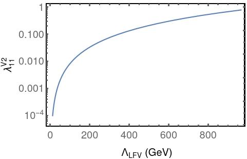
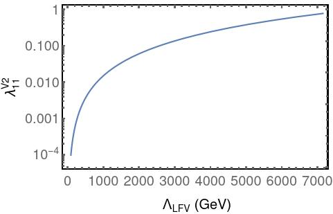
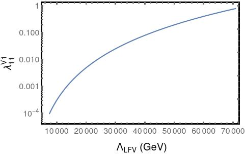
In the case of scalar operators, the constrain on the lepton flavour violation scale (ΛL​F​V\Lambda_{LFV}) is very weak due to an additional electron Yukawa coupling as given in Table. 3. Whereas, vector operators are not suppressed and Fig. 1 shows the limits on ΛL​F​V\Lambda_{LFV} from BR(μ−→e−​e+​e−)e​x​p(\mu^{-}\rightarrow e^{-}e^{+}e^{-})_{exp} for different values of λ11V​2\lambda^{V2}_{11} in both minimal and extended field content scenarios. ΛL​F​V\Lambda_{LFV} is more constrained in the case of extended field content scenario since Δ\Delta is proportional to the mass of the neutrino mνm_{\nu} whereas, in minimal field scenario, it is proportional to the square of neutrino mass (mν2m^{2}_{\nu}).

Refer to caption
(a) (a) Minimal field content scenario
Refer to caption
(b) (b) Extended field content scenario
Figure 1: The plots show limits on ΛL​F​V\Lambda_{LFV} from BR(μ−→e−​e+​e−)e​x​p(\mu^{-}\rightarrow e^{-}e^{+}e^{-})_{exp} for different values of λ11V​2\lambda^{V2}_{11} in both minimal and extended field content scenario. The region below the curve is allowed by the experiments

π0→e+​μ−:\pi^{0}\rightarrow e^{+}\mu^{-}:
The operators that contribute to π0→e+​μ−\pi^{0}\rightarrow e^{+}\mu^{-} are:

𝒞μ​e​d​dS​1​𝒪μ​e​d​dS​1=\displaystyle\mathcal{C}^{S1}_{\mu edd}\mathcal{O}^{S1}_{\mu edd}= (μ¯L​{Δ†​Ye†}21​eR)​(d¯R​λ11S​1​dL)\displaystyle\Big(\bar{\mu}_{L}\penalty\ \{\Delta^{\dagger}Y^{\dagger}_{e}\}_{21}\penalty\ e_{R}\Big)(\bar{d}_{R}\penalty\ \lambda^{S1}_{11}\penalty\ d_{L})
𝒞μ​e​u​uS​2​𝒪μ​e​u​uS​2=\displaystyle\mathcal{C}^{S2}_{\mu euu}\mathcal{O}^{S2}_{\mu euu}= (μ¯L​{Δ†​Ye†}21​eR)​(u¯R​λ11S​2​uL)\displaystyle\Big(\bar{\mu}_{L}\penalty\ \{\Delta^{\dagger}Y^{\dagger}_{e}\}_{21}\penalty\ e_{R}\Big)(\bar{u}_{R}\penalty\ \lambda^{S2}_{11}\penalty\ u_{L})
𝒞μ​e​q​qV​1​𝒪μ​e​q​qV​1=\displaystyle\mathcal{C}^{V1}_{\mu eqq}\mathcal{O}^{V1}_{\mu eqq}= (μ¯L​γμ​Δ21​eL)​(u¯L​γμ​λ11V​1​uL+d¯L​γμ​λ11V​1​dL)\displaystyle\Big(\bar{\mu}_{L}\penalty\ \gamma^{\mu}\Delta_{21}\penalty\ e_{L}\Big)(\bar{u}_{L}\penalty\ \gamma_{\mu}\lambda^{V1}_{11}\penalty\ u_{L}+\bar{d}_{L}\penalty\ \gamma_{\mu}\lambda^{V1}_{11}\penalty\ d_{L})
𝒞μ​e​u​uV​3​𝒪μ​e​u​uV​3=\displaystyle\mathcal{C}^{V3}_{\mu euu}\mathcal{O}^{V3}_{\mu euu}= (μ¯L​γμ​Δ21​eL)​(u¯R​γμ​λ11V​3​uR)\displaystyle\Big(\bar{\mu}_{L}\penalty\ \gamma^{\mu}\Delta_{21}\penalty\ e_{L}\Big)(\bar{u}_{R}\penalty\ \gamma_{\mu}\lambda^{V3}_{11}\penalty\ u_{R})
𝒞μ​e​d​dV​4​𝒪μ​e​d​dV​4=\displaystyle\mathcal{C}^{V4}_{\mu edd}\mathcal{O}^{V4}_{\mu edd}= (μ¯L​γμ​Δ21​eL)​(d¯R​γμ​λ11V​4​dR)\displaystyle\Big(\bar{\mu}_{L}\penalty\ \gamma^{\mu}\Delta_{21}\penalty\ e_{L}\Big)(\bar{d}_{R}\penalty\ \gamma_{\mu}\lambda^{V4}_{11}\penalty\ d_{R}) (36)

The branching ratio of π0→e+​μ−\pi^{0}\rightarrow e^{+}\mu^{-} in case of scalar operator, given in Eq.(II.2), becomes,

BR​(π0→e+​μ−)=|pμ|π0​μ​e8​π​mπ2​τπ0​B02​F024​|𝒞μ​e​d​dS​1+𝒞μ​e​u​uS​2|2ΛL​F​V4​(mπ2−(me+mμ)2),\displaystyle\text{BR}(\pi^{0}\rightarrow e^{+}\mu^{-})=\frac{{|p_{\mu}|}_{\pi^{0}\mu e}}{8\pi m_{\pi}^{2}}\frac{\tau_{\pi^{0}}B_{0}^{2}F_{0}^{2}}{4}\frac{|\mathcal{C}^{S1}_{\mu edd}+\mathcal{C}^{S2}_{\mu euu}|^{2}}{\Lambda^{4}_{LFV}}(m_{\pi}^{2}-(m_{e}+m_{\mu})^{2})\ ,
|𝒞μ​e​d​dS​1+𝒞μ​e​u​uS​2|2ΛL​F​V4<4.1×10⁻¹³​GeV−4,\displaystyle\frac{|\mathcal{C}^{S1}_{\mu edd}+\mathcal{C}^{S2}_{\mu euu}|^{2}}{\Lambda^{4}_{LFV}}<4.1\times 10^{-13}\text{GeV}^{-4}\ , (37)

where τπ0=8.43×10⁻¹⁷​s\tau_{\pi^{0}}=8.43\times 10^{-17}s is the mean life time of pion. The branching ratio in terms of the Wilson coefficients of vector operator Thomas et al. 2022 is given by,

BR​(π0→e+​μ−)=|pμ|π0​μ​e8​π​mπ2​τπ0​F024​|𝒞μ​e​u​uV​3−𝒞μ​e​d​dV​4+𝒞μ​e​d​dV​1−𝒞μ​e​u​uV​1|2ΛL​F​V4​(mπ2​(mμ2+me2)−(mμ2−me2)2),\displaystyle\text{BR}(\pi^{0}\rightarrow e^{+}\mu^{-})=\frac{{|p_{\mu}|}_{\pi^{0}\mu e}}{8\pi m_{\pi}^{2}}\frac{\tau_{\pi^{0}}F_{0}^{2}}{4}\frac{|\mathcal{C}^{V3}_{\mu euu}-\mathcal{C}^{V4}_{\mu edd}+\mathcal{C}^{V1}_{\mu edd}-\mathcal{C}^{V1}_{\mu euu}|^{2}}{\Lambda^{4}_{LFV}}(m_{\pi}^{2}(m_{\mu}^{2}+m_{e}^{2})-(m_{\mu}^{2}-m_{e}^{2})^{2})\ ,
|𝒞μ​e​u​uV​3−𝒞μ​e​d​dV​4+𝒞μ​e​d​dV​1−𝒞μ​e​u​uV​1|2ΛL​F​V4<2.67×10⁻¹⁰​GeV−4.\displaystyle\frac{|\mathcal{C}^{V3}_{\mu euu}-\mathcal{C}^{V4}_{\mu edd}+\mathcal{C}^{V1}_{\mu edd}-\mathcal{C}^{V1}_{\mu euu}|^{2}}{\Lambda^{4}_{LFV}}<2.67\times 10^{-10}\text{GeV}^{-4}\ . (38)

We find that ΛL​F​V\Lambda_{LFV} is weakly constrained by BR(π0→e+​μ−)e​x​p(\pi^{0}\rightarrow e^{+}\mu^{-})_{exp} for both scalar operator and vector operator in minimal and extended field content scenarios.

KL→μ+​e−:K_{L}\rightarrow\mu^{+}e^{-}:
The operators that contribute to KL→μ+​e−K_{L}\rightarrow\mu^{+}e^{-} are:

𝒞e​μ​d​sS​1​𝒪e​μ​d​sS​1=\displaystyle\mathcal{C}^{S1}_{e\mu ds}\mathcal{O}^{S1}_{e\mu ds}= (e¯L​{Δ†​Ye†}12​μR)​(d¯R​λ12S​1​sL)\displaystyle\Big(\bar{e}_{L}\penalty\ \{\Delta^{\dagger}Y^{\dagger}_{e}\}_{12}\penalty\ \mu_{R}\Big)(\bar{d}_{R}\penalty\ \lambda^{S1}_{12}\penalty\ s_{L})
𝒞e​μ​s​dS​1​𝒪e​μ​s​dS​1=\displaystyle\mathcal{C}^{S1}_{e\mu sd}\mathcal{O}^{S1}_{e\mu sd}= (e¯L​{Δ†​Ye†}12​μR)​(s¯R​λ21S​1​dL)\displaystyle\Big(\bar{e}_{L}\penalty\ \{\Delta^{\dagger}Y^{\dagger}_{e}\}_{12}\penalty\ \mu_{R}\Big)(\bar{s}_{R}\penalty\ \lambda^{S1}_{21}\penalty\ d_{L})
𝒞e​μ​q​qV​1​𝒪e​μ​q​qV​1=\displaystyle\mathcal{C}^{V1}_{e\mu qq}\mathcal{O}^{V1}_{e\mu qq}= (e¯L​γμ​Δ12​μL)​(d¯L​γμ​λ12V​1​sL+s¯L​γμ​λ21V​1​dL)\displaystyle\Big(\bar{e}_{L}\penalty\ \gamma^{\mu}\Delta_{12}\penalty\ \mu_{L}\Big)(\bar{d}_{L}\penalty\ \gamma_{\mu}\lambda^{V1}_{12}\penalty\ s_{L}+\bar{s}_{L}\penalty\ \gamma_{\mu}\lambda^{V1}_{21}\penalty\ d_{L})
𝒞e​μ​q​qV​4​𝒪e​μ​q​qV​1=\displaystyle\mathcal{C}^{V4}_{e\mu qq}\mathcal{O}^{V1}_{e\mu qq}= (e¯L​γμ​Δ12​μL)​(d¯L​γμ​λ12V​4​sL+s¯L​γμ​λ21V​4​dL)\displaystyle\Big(\bar{e}_{L}\penalty\ \gamma^{\mu}\Delta_{12}\penalty\ \mu_{L}\Big)(\bar{d}_{L}\penalty\ \gamma_{\mu}\lambda^{V4}_{12}\penalty\ s_{L}+\bar{s}_{L}\penalty\ \gamma_{\mu}\lambda^{V4}_{21}\penalty\ d_{L}) (39)

We assume that λ12S​1=λ21S​1,λ12V​1=λ21V​1\lambda^{S1}_{12}=\lambda^{S1}_{21},\lambda^{V1}_{12}=\lambda^{V1}_{21} and λ12V​4=λ21V​4\lambda^{V4}_{12}=\lambda^{V4}_{21}. The branching ratio in case of scalar operator, given in Eq.(II.1), now becomes,

BR​(KL→μ+​e−)=|pμ|KL​μ​e8​π​mKL02​τKL​B02​F024​|(𝒞e​μ​d​sS​1ΛL​F​V2​α−𝒞e​μ​s​dS​1ΛL​F​V2​β)|2​(mKL02−(mμ+me)2),\displaystyle\text{BR}(K_{L}\rightarrow\mu^{+}e^{-})=\frac{{|p_{\mu}|}_{K_{L}\mu e}}{8\pi m_{K^{0}_{L}}^{2}}\frac{\tau_{K_{L}}B_{0}^{2}F_{0}^{2}}{4}\left|\left(\frac{\mathcal{C}^{S1}_{e\mu ds}}{\Lambda^{2}_{LFV}\alpha}-\frac{\mathcal{C}^{S1}_{e\mu sd}}{\Lambda^{2}_{LFV}\beta}\right)\right|^{2}(m_{K^{0}_{L}}^{2}-(m_{\mu}+m_{e})^{2})\ ,
|𝒞e​μ​d​sS​1|2ΛL​F​V4<2.2×10⁻²⁰​GeV−4,\displaystyle\frac{|\mathcal{C}^{S1}_{e\mu ds}|^{2}}{\Lambda^{4}_{LFV}}<2.2\times 10^{-20}\text{GeV}^{-4}\ , (40)

where τKL=5.116×10⁻⁸​s\tau_{K_{L}}=5.116\times 10^{-8}s is the mean life time of KLK_{L}. And, the branching ratio in case of vector operator Thomas et al. 2022 becomes,

BR​(KL→e+​μ−)=|pμ|KL​μ​e8​π​mKL02​τKL​F024​|(−𝒞e​μ​d​sV​1ΛL​F​V2​α+𝒞e​μ​s​dV​1ΛL​F​V2​β+𝒞e​μ​d​sV​4ΛL​F​V2​α−𝒞e​μ​s​dV​4ΛL​F​V2​β)|2​(mKL02​(mμ2+me2)−(mμ2−me2)2),\displaystyle\text{BR}(K_{L}\rightarrow e^{+}\mu^{-})=\frac{{|p_{\mu}|}_{K_{L}\mu e}}{8\pi m_{K^{0}_{L}}^{2}}\frac{\tau_{K_{L}}F_{0}^{2}}{4}\left|\left(-\frac{\mathcal{C}^{V1}_{e\mu ds}}{\Lambda^{2}_{LFV}\alpha}+\frac{\mathcal{C}^{V1}_{e\mu sd}}{\Lambda^{2}_{LFV}\beta}+\frac{\mathcal{C}^{V4}_{e\mu ds}}{\Lambda^{2}_{LFV}\alpha}-\frac{\mathcal{C}^{V4}_{e\mu sd}}{\Lambda^{2}_{LFV}\beta}\right)\right|^{2}(m_{K^{0}_{L}}^{2}(m_{\mu}^{2}+m_{e}^{2})-(m_{\mu}^{2}-m_{e}^{2})^{2})\ ,
|(−𝒞e​μ​d​sV​1ΛL​F​V2​α+𝒞e​μ​s​dV​1ΛL​F​V2​β+𝒞e​μ​d​sV​4ΛL​F​V2​α−𝒞e​μ​s​dV​4ΛL​F​V2​β)|2<2.81×10⁻²²​GeV−4.\displaystyle\left|\left(-\frac{\mathcal{C}^{V1}_{e\mu ds}}{\Lambda^{2}_{LFV}\alpha}+\frac{\mathcal{C}^{V1}_{e\mu sd}}{\Lambda^{2}_{LFV}\beta}+\frac{\mathcal{C}^{V4}_{e\mu ds}}{\Lambda^{2}_{LFV}\alpha}-\frac{\mathcal{C}^{V4}_{e\mu sd}}{\Lambda^{2}_{LFV}\beta}\right)\right|^{2}<2.81\times 10^{-22}\text{GeV}^{-4}\ . (41)
Refer to caption
(a) (a) Vector operator minimal field content scenario
Refer to caption
(b) (b) Vector operator extended field content scenario
Refer to caption
(c) (c) Vector operator minimal field content scenario
Refer to caption
(d) (d) Vector operator extended field content scenario
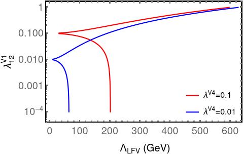
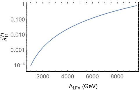
Figure 2: The plots (a) & (b) show limits on ΛL​F​V\Lambda_{LFV} from KL→μ+​e−K_{L}\rightarrow\mu^{+}e^{-} treating λ12V​1\lambda^{V1}_{12} as a variable while keeping λ12V​4\lambda^{V4}_{12} fixed. While the plots (c) & (d) shows the limit on ΛL​F​V\Lambda_{LFV} keeping the combination λ12V​1−λ12V​4\lambda^{V1}_{12}-\lambda^{V4}_{12} as the variable. In the plots (a) & (b), the red line corresponds to limits for benchmark value of λ12V​4=0.1\lambda^{V4}_{12}=0.1 and blue line corresponds to λ12V​4=0.01\lambda^{V4}_{12}=0.01. Note that there is a complete cancellation of Wilson coefficients, given in Eq. (III.3), for λ12V​1=λ12V​4\lambda^{V1}_{12}=\lambda^{V4}_{12}, which leads to a beak like structure of the function. Moreover, Eq. (III.3) behaves differently for λ12V​1\lambda^{V1}_{12} values above and below this point. While above this point 𝒞V​1\mathcal{C}^{V1} is dominant and ΛL​F​V\Lambda_{LFV} increases with λ12V​1\lambda^{V1}_{12}, below this point, 𝒞V​4\mathcal{C}^{V4} becomes dominant.

The limit on ΛL​F​V\Lambda_{LFV} from BR(KL→μ+​e−)e​x​p(K_{L}\rightarrow\mu^{+}e^{-})_{exp} in vector operator scenario for different values of λ\lambda is shown in Fig.2. In the case of scalar operator ΛL​F​V\Lambda_{LFV} is weakly constrained by the BR(KL→μ+​e−)e​x​p(K_{L}\rightarrow\mu^{+}e^{-})_{exp}.

μ​N→e​N:\mu N\rightarrow eN:
The operators that contribute to μ​N→e​N\mu N\rightarrow eN are:

𝒞e​μ​d​dS​1​𝒪e​μ​d​dS​1=\displaystyle\mathcal{C}^{S1}_{e\mu dd}\mathcal{O}^{S1}_{e\mu dd}= (e¯L​{Δ†​Ye†}12​μR)​(d¯R​λ11S​1​dL)\displaystyle\Big(\bar{e}_{L}\penalty\ \{\Delta^{\dagger}Y^{\dagger}_{e}\}_{12}\penalty\ \mu_{R}\Big)(\bar{d}_{R}\penalty\ \lambda^{S1}_{11}\penalty\ d_{L})
𝒞e​μ​u​uS​2​𝒪e​μ​u​uS​2=\displaystyle\mathcal{C}^{S2}_{e\mu uu}\mathcal{O}^{S2}_{e\mu uu}= (e¯L​{Δ†​Ye†}12​μR)​(u¯R​λ11S​2​uL)\displaystyle\Big(\bar{e}_{L}\penalty\ \{\Delta^{\dagger}Y^{\dagger}_{e}\}_{12}\penalty\ \mu_{R}\Big)(\bar{u}_{R}\penalty\ \lambda^{S2}_{11}\penalty\ u_{L})
𝒞e​μ​q​qV​1​𝒪e​μ​q​qV​1=\displaystyle\mathcal{C}^{V1}_{e\mu qq}\mathcal{O}^{V1}_{e\mu qq}= (e¯L​γμ​Δ12​μL)​(u¯L​γμ​λ11V​1​uL+d¯L​γμ​λ11V​1​dL)\displaystyle\Big(\bar{e}_{L}\penalty\ \gamma^{\mu}\Delta_{12}\penalty\ \mu_{L}\Big)(\bar{u}_{L}\penalty\ \gamma_{\mu}\lambda^{V1}_{11}\penalty\ u_{L}+\bar{d}_{L}\penalty\ \gamma_{\mu}\lambda^{V1}_{11}\penalty\ d_{L})
𝒞e​μ​u​uV​3​𝒪e​μ​u​uV​3=\displaystyle\mathcal{C}^{V3}_{e\mu uu}\mathcal{O}^{V3}_{e\mu uu}= (e¯L​γμ​Δ12​μL)​(u¯R​γμ​λ11V​3​uR)\displaystyle\Big(\bar{e}_{L}\penalty\ \gamma^{\mu}\Delta_{12}\penalty\ \mu_{L}\Big)(\bar{u}_{R}\penalty\ \gamma_{\mu}\lambda^{V3}_{11}\penalty\ u_{R})
𝒞e​μ​d​dV​4​𝒪e​μ​d​dV​4=\displaystyle\mathcal{C}^{V4}_{e\mu dd}\mathcal{O}^{V4}_{e\mu dd}= (e¯L​γμ​Δ12​μL)​(d¯R​γμ​λ11V​4​dR)\displaystyle\Big(\bar{e}_{L}\penalty\ \gamma^{\mu}\Delta_{12}\penalty\ \mu_{L}\Big)(\bar{d}_{R}\penalty\ \gamma_{\mu}\lambda^{V4}_{11}\penalty\ d_{R})

The best limit on μ→e\mu\rightarrow e conversion comes from the SINDRUM II collaboration, which puts a limit on BR(μ​T​i→e​T​i)e​x​p<6.1×10⁻¹³(\mu Ti\rightarrow eTi)_{exp}<6.1\times 10^{-13} Kaulard et al. 1998. The branching ratio of μ​N→e​N\mu N\rightarrow eN conversion in the notation of Ref. Kitano et al. 2002,

BR​(μ​N→e​N)\displaystyle\text{BR}(\mu N\rightarrow eN) =\displaystyle= 2​GF2wc​a​p​t​(|g~L​S(p)​S(p)+g~L​S(n)​S(n)+g~L​V(p)​V(p)+g~L​V(n)​V(n)|2CLOSE\displaystyle\displaystyle\frac{2G^{2}_{F}}{w_{capt}}\Bigg(|\tilde{g}^{(p)}_{LS}S^{(p)}+\tilde{g}^{(n)}_{LS}S^{(n)}+\tilde{g}^{(p)}_{LV}V^{(p)}+\tilde{g}^{(n)}_{LV}V^{(n)}|^{2} (43)
+\displaystyle+ OPEN|g~R​S(p)​S(p)+g~R​S(n)​S(n)+g~R​V(p)​V(p)+g~R​V(n)​V(n)|2)\displaystyle\displaystyle|\tilde{g}^{(p)}_{RS}S^{(p)}+\tilde{g}^{(n)}_{RS}S^{(n)}+\tilde{g}^{(p)}_{RV}V^{(p)}+\tilde{g}^{(n)}_{RV}V^{(n)}|^{2}\Bigg)

where,

g~L​S,R​S(p)\displaystyle\tilde{g}_{LS,RS}^{(p)} =\displaystyle= ∑qGS(q,p)​gL​S,R​S​(q),\displaystyle\sum_{q}G_{S}^{(q,p)}\ g_{LS,RS(q)}\ ,
g~L​S,R​S(n)\displaystyle\tilde{g}_{LS,RS}^{(n)} =\displaystyle= ∑qGS(q,n)​gL​S,R​S​(q),\displaystyle\sum_{q}G_{S}^{(q,n)}\ g_{LS,RS(q)}\ ,
g~L​V,R​V(p)\displaystyle\tilde{g}_{LV,RV}^{(p)} =\displaystyle= 2​gL​V,R​V​(u)+gL​V,R​V​(d),\displaystyle 2g_{LV,RV(u)}+g_{LV,RV(d)}\ ,
g~L​V,R​V(n)\displaystyle\tilde{g}_{LV,RV}^{(n)} =\displaystyle= gL​V,R​V​(u)+2​gL​V,R⁡(d).\displaystyle g_{LV,RV(u)}+2g_{LV,R(d)}\ . (44)
Refer to caption
(a) (a) Scalar operator minimal field content scenario
Refer to caption
(b) (b) Vector operator minimal field content scenario
Refer to caption
(c) (c) Scalar operator extended field content scenario
Refer to caption
(d) (d) Vector operator extended field content scenario
Figure 3: The plots show limits on ΛL​F​V\Lambda_{LFV} from BR(μ​T​i→e​T​i)(\mu Ti\rightarrow eTi) for different values of λ11S​2/λ11V​1\lambda^{S2}_{11}/\lambda^{V1}_{11} in scalar and vector operators in minimal and extended field content scenarios. The region below the curve is allowed by the experiments

For scalar operator we consider a scenario when λS​1=0\lambda^{S1}=0 and λS​2≠0\lambda^{S2}\neq 0, in this case 𝒞e​μ​d​dS​2=GF2​2​gL​S​(d)\mathcal{C}^{S2}_{e\mu dd}=\frac{G_{F}}{2\sqrt{2}}g_{LS(d)},

BR​(μ​T​i→e​T​i)=16wc​a​p​t​(GS(d,p)​S(p)+GS(d,n)​S(n))2​|𝒞e​μ​d​dS​2|2ΛL​F​V4\displaystyle\text{BR}(\mu Ti\rightarrow eTi)=\frac{16}{w_{capt}}(G^{(d,p)}_{S}S^{(p)}+G^{(d,n)}_{S}S^{(n)})^{2}\frac{|\mathcal{C}^{S2}_{e\mu dd}|^{2}}{\Lambda^{4}_{LFV}}
|𝒞e​μ​d​dS​2|2ΛL​F​V4<1.37×10⁻²⁵​GeV−4\displaystyle\frac{|\mathcal{C}^{S2}_{e\mu dd}|^{2}}{\Lambda^{4}_{LFV}}<1.37\times 10^{-25}\text{GeV}^{-4} (45)

In the case of a vector operator GF2​gL​V​(d)=(𝒞e​μ​d​dV​1+𝒞e​μ​d​dV​4),GF2​gL​V​(u)=(𝒞e​μ​u​uV​1+𝒞e​μ​u​uV​3)\frac{G_{F}}{\sqrt{2}}g_{LV(d)}=(\mathcal{C}^{V1}_{e\mu dd}+\mathcal{C}^{V4}_{e\mu dd}),\frac{G_{F}}{\sqrt{2}}g_{LV(u)}=(\mathcal{C}^{V1}_{e\mu uu}+\mathcal{C}^{V3}_{e\mu uu}),

BR​(μ​T​i→e​T​i)=36wc​a​p​t​(V(p)+V(n))2​|𝒞e​μ​d​dV​1|2ΛL​F​V4\displaystyle\text{BR}(\mu Ti\rightarrow eTi)=\frac{36}{w_{capt}}(V^{(p)}+V^{(n)})^{2}\frac{|\mathcal{C}^{V1}_{e\mu dd}|^{2}}{\Lambda^{4}_{LFV}}
|𝒞e​μ​d​dV​1|2ΛL​F​V4<2.94×10⁻²⁵​GeV−4\displaystyle\frac{|\mathcal{C}^{V1}_{e\mu dd}|^{2}}{\Lambda^{4}_{LFV}}<2.94\times 10^{-25}\text{GeV}^{-4} (46)

Here we have assumed λ11V​1=λ11V​4=λ11V​3\lambda^{V1}_{11}=\lambda^{V4}_{11}=\lambda^{V3}_{11} for simplicity. The constants that have used to compute the above expressions are listed in Table. 6.

wc​a​pw_{cap} 1.7047×10181.7047\times 10^{18} GeV S(n)S^{(n)} 0.0435​mμ5/20.0435\penalty\ m^{5/2}_{\mu}
GS(d,p)G^{(d,p)}_{S} 4.34.3 V(p)V^{(p)} 0.0396​mμ5/20.0396\penalty\ m^{5/2}_{\mu}
GS(d,n)G^{(d,n)}_{S} 5.15.1 V(n)V^{(n)} 0.0468​mμ5/20.0468\penalty\ m^{5/2}_{\mu}
S(p)S^{(p)} 0.0368​mμ5/20.0368\penalty\ m^{5/2}_{\mu}
Table 6: Various constants used in Eq. (III.3) and (III.3) Kitano et al. 2002.

Fig. 3 shows the limit on ΛL​F​V\Lambda_{LFV} from BR(μ​T​i→e​T​i)(\mu Ti\rightarrow eTi) for different values of λ11S​2/λ11V​1\lambda^{S2}_{11}/\lambda^{V1}_{11} in scalar and vector operator scenarios. We see that among all the lepton flavour violating decays considered, the best limit on ΛL​F​V\Lambda_{LFV} arise from the vector operator. This is expected since vector operators are 𝒪⁡(mν2)\mathcal{O}(m_{\nu}^{2}), were as the scalar operators are 𝒪⁡(mν2​me)\mathcal{O}(m_{\nu}^{2}m_{e}).

IV Conclusion

Tri-bimaximal-Cabibbo mixing ansatz is a possible venue for new physics that can contribute towards charged lepton flavour violation. Importantly, this ansatz brings back the thought to be dead, but theoretically well-motivated, Tri-bimaximal mixing in the neutrino sector. In this paper, we investigate the LFV in charged lepton sector induced by TBC mixing in the context of various lepton flavour violating decays like μ→e​e​e\mu\to eee, μ→e​γ\mu\rightarrow e\gamma, π0→μ​e\pi^{0}\to\mu e, KL→μ​eK_{L}\to\mu e and μ​N→e​N\mu N\to eN. A model-independent analysis using the effective field theory operators revealed that if we assume TBC mixing to be the only source of LFV in charged lepton sector then it can be ruled out by current limits on lepton flavour violating decays KL→μ+​e−K_{L}\rightarrow\mu^{+}e^{-}, π0→e+​μ−\pi^{0}\rightarrow e^{+}\mu^{-} and μ→e​γ\mu\rightarrow e\gamma.

Whereas, the MFV hypothesis protects the TBC mixing ansatz from these lepton flavour violating decays, naturally, making the NP available at LHC. We introduce MFV only in lepton sector and show that this suppresses the large flavour violations induced by the Cabibbo mixing in the first two generations of the charged leptons. In the MFV hypothesis, we have considered two scenarios. One with the minimal field content and the other including right-handed neutrinos namely, the extended field content. In the extended field content scenario, instead of introducing spurions, we have assumed the right-handed Majorana mass terms to be diagonal. With this, we have derived the limits on ΛL​F​V\Lambda_{LFV} for both minimal and extended scenarios. In Table 7 and 8 we summarise the limit on ΛL​F​V\Lambda_{LFV}. The strongest constrain on ΛL​F​V\Lambda_{LFV} arises from BR(μ​T​i→e​T​i)(\mu Ti\rightarrow eTi) and μ→e​γ\mu\to e\gamma. Assuming 𝒪⁡(1)\mathcal{O}(1) couplings in the quark sector, this process bounds the cut-off scale to be ΛL​F​V≳10\Lambda_{LFV}\gtrsim 10 TeV in the minimal content scenario. Instead, if we assume a slightly lower coupling of NP in the quark sector, this limit could be relaxed to ΛL​F​V≳4\Lambda_{LFV}\gtrsim 4 TeV. On the other hand, we find that the constraints in extended field content scenario are much stronger than the minimal field content scenario. The limit on ΛL​F​V\Lambda_{LFV} is now >75>75 TeV for 𝒪⁡(1)\mathcal{O}(1) coupling in the quark sector, while it relaxes to 3131 TeV on assuming more natural values of the couplings. This is expected since Δ\Delta, given in Table. 3, is proportional to mνm_{\nu} in extended field scenarios whereas in minimal field scenario it is proportional to mν2m^{2}_{\nu}. We also note that scalar operators are further suppressed compared to vector operators due to the presence of an additional charged lepton Yukawa coupling.

Though the dipole operator is highly constraining, note that this operator arises at 1-loop in Beyond Standard Model (BSM). On the other hand, μ→e​e​e\mu\to eee is a pure leptonic tree-level BSM process and hence, it is important that we compute them. With this consideration, we have found that in minimal field content scenario, μ→e​e​e\mu\to eee constrains the new physics to ΛL​F​V≳1\Lambda_{LFV}\gtrsim 1 TeV, while in extended field scenario, they become ΛL​F​V≳8\Lambda_{LFV}\gtrsim 8 TeV.

Thus, assuming MFV, the lepton flavour violating new physics is not only closer to the scale of experiments, but also the Tri-bimaximal neutrino mixing matrix is safe from the reactor angle measurement.

Observables Scenario Limit on ΛL​F​V\Lambda_{LFV} (TeV) Scenario Limit on ΛL​F​V\Lambda_{LFV} (TeV)
BR(π0→e+​μ−)(\pi^{0}\rightarrow e^{+}\mu^{-}) λ11S​1=1λ11S​2=0.1\lambda^{S1}_{11}=1\penalty\ \penalty\ \lambda^{S2}_{11}=0.1 1×10−51\times 10^{-5} λ11S​1=mdvλ11S​2=muv\lambda^{S1}_{11}=\frac{m_{d}}{v}\penalty\ \penalty\ \lambda^{S2}_{11}=\frac{m_{u}}{v} 4.2×10−84.2\times 10^{-8}
λ11V​3=1λ11V​4=0.1\lambda^{V3}_{11}=1\penalty\ \penalty\ \lambda^{V4}_{11}=0.1 1.2×10−31.2\times 10^{-3} λ11V​3=muvλ11V​4=mdv\lambda^{V3}_{11}=\frac{m_{u}}{v}\penalty\ \penalty\ \lambda^{V4}_{11}=\frac{m_{d}}{v} 4.9×10−64.9\times 10^{-6}
BR(μ−→e−​e+​e−)(\mu^{-}\rightarrow e^{-}e^{+}e^{-}) λ11S​3=1\lambda^{S3}_{11}=1 1.58×10−21.58\times 10^{-2} λ11S​3=c12e\lambda^{S3}_{11}=c^{e}_{12} 1.56×10−21.56\times 10^{-2}
λ11V​2=1\lambda^{V2}_{11}=1 1.083 λ11V​2=c12e\lambda^{V2}_{11}=c^{e}_{12} 1.069
BR (KL→μ+​e−)(K_{L}\rightarrow\mu^{+}e^{-}) λ12S​1=1\lambda^{S1}_{12}=1 0.01 λ12S​1=msv\lambda^{S1}_{12}=\frac{m_{s}}{v} 0.24×10−30.24\times 10^{-3}
λ12V​1=1λ12V​4=0.1\lambda^{V1}_{12}=1\penalty\ \penalty\ \lambda^{V4}_{12}=0.1 0.274 λ12V​1=msvλ12V​4=msv\lambda^{V1}_{12}=\frac{m_{s}}{v}\penalty\ \penalty\ \lambda^{V4}_{12}=\frac{m_{s}}{v} 8.6×10−28.6\times 10^{-2}
BR(μ​T​i→e​T​i)(\mu Ti\rightarrow eTi) λ11S​2=1\lambda^{S2}_{11}=1 0.301 λ11S​2=mdv\lambda^{S2}_{11}=\frac{m_{d}}{v} 1.6×10−31.6\times 10^{-3}
λ11V​1=1\lambda^{V1}_{11}=1 10.126 λ11V​1=mdv\lambda^{V1}_{11}=\frac{m_{d}}{v} 0.728
BR(μ→e​γ)(\mu\rightarrow e\gamma) - 4.17 - 4.17
Table 7: Limit on ΛL​F​V\Lambda_{LFV} from different lepton flavour violating decays in minimal field content scenario.
Observables Scenario Limit on ΛL​F​V\Lambda_{LFV} (TeV) Scenario Limit on ΛL​F​V\Lambda_{LFV} (TeV)
BR(π0→e+​μ−)(\pi^{0}\rightarrow e^{+}\mu^{-}) λ11S​1=1λ11S​2=0.1\lambda^{S1}_{11}=1\penalty\ \penalty\ \lambda^{S2}_{11}=0.1 7.8×10−57.8\times 10^{-5} λ11S​1=mdvλ11S​2=muv\lambda^{S1}_{11}=\frac{m_{d}}{v}\penalty\ \penalty\ \lambda^{S2}_{11}=\frac{m_{u}}{v} 3.1×10−73.1\times 10^{-7}
λ11S​1=1λ11S​2=0.1\lambda^{S1}_{11}=1\penalty\ \penalty\ \lambda^{S2}_{11}=0.1 9.21×10−39.21\times 10^{-3} λ11V​3=muvλ11V​4​mdv\lambda^{V3}_{11}=\frac{m_{u}}{v}\penalty\ \penalty\ \lambda^{V4}_{11}\frac{m_{d}}{v} 3.6×10−53.6\times 10^{-5}
BR(μ−→e−​e+​e−)(\mu^{-}\rightarrow e^{-}e^{+}e^{-}) λ11S​3=1\lambda^{S3}_{11}=1 0.117 λ11S​3=c12e\lambda^{S3}_{11}=c^{e}_{12} 0.115
λ11V​2=1\lambda^{V2}_{11}=1 8.019 λ11V​2=c12e\lambda^{V2}_{11}=c^{e}_{12} 7.915
BR (KL→μ+​e−)(K_{L}\rightarrow\mu^{+}e^{-}) λ12S​1=1\lambda^{S1}_{12}=1 0.078 λ12S​1=msv\lambda^{S1}_{12}=\frac{m_{s}}{v} 1.8×10−31.8\times 10^{-3}
λ12V​1=1λ12V​4=0.1\lambda^{V1}_{12}=1\penalty\ \penalty\ \lambda^{V4}_{12}=0.1 2 λ12V​1=msvλ12V​4=msv\lambda^{V1}_{12}=\frac{m_{s}}{v}\penalty\ \penalty\ \lambda^{V4}_{12}=\frac{m_{s}}{v} 0.636
BR(μ​T​i→e​T​i)(\mu Ti\rightarrow eTi) λ11S​2=1\lambda^{S2}_{11}=1 1.577 λ11S​2=mdv\lambda^{S2}_{11}=\frac{m_{d}}{v} 8.1×10−38.1\times 10^{-3}
λ11V​1=1\lambda^{V1}_{11}=1 74.97 λ11V​1=mdv\lambda^{V1}_{11}=\frac{m_{d}}{v} 5.397
BR(μ→e​γ)(\mu\rightarrow e\gamma) - 30.94 - 30.94
Table 8: Limit on ΛL​F​V\Lambda_{LFV} from different lepton flavour violating decays in extended field content scenario.
Acknowledgements.
M.T.A. acknowledges the financial support of DST through INSPIRE Faculty grant DST/INSPIRE/04/2019/002507.

References