Wobble control of a pendulum actuated spherical robot

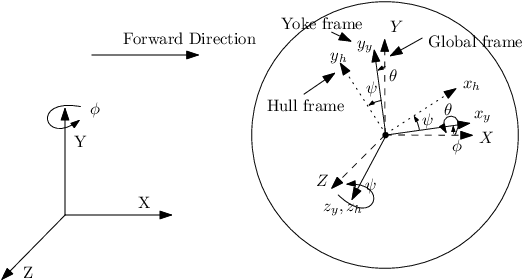
This work is based on four reference frames as shown in figure 2: a global inertial frame fixed to the ground ($\mathbf{G}$), and the three frames attached to the yoke ($\mathbf{Y}$), pendulum ($\mathbf{P}$) and the hull ($\mathbf{H}$) respectively with their origins at the geometric center of the hull. The yoke frame $\mathbf{Y}$ is defined to meet the following constraints: (1) The $z$-axis of the yoke is always aligned with the $z$-axis of the hull, and (2) The $x$-axis of the yoke frame lies in the global $XZ$-plane, i.e., it always remains parallel to the ground.

The orientation of the hull at any given instant is characterized by three $YXZ$ Euler angles $\phi$, $\theta$, and $\psi$. The orientation of the pendulum requires another angle $\beta$ due to an additional degree of freedom. The transformation between frames happens as follows :

• •

  Intermediate Frame ($\mathbf{I}$): $\mathbf{G}$ is rotated along its $Y$-axis by angle $\phi$ to obtain $\mathbf{I}$ as shown in Figure 3(a).

• •

  Yoke frame ($\mathbf{Y}$): $\mathbf{I}$ is rotated along its local $x$-axis $x_{i}$ by angle $\theta$ to obtain $\mathbf{Y}$ as shown in Figure 3(b).

• •

  Pendulum frame ($\mathbf{P}$): $\mathbf{Y}$ is rotated along its local $x$-axis $x_{y}$ by angle $\beta$ to obtain $\mathbf{P}$ as shown in Figure 3(c). Note that the angle made by the pendulum with the vertical axis $Y$ is ($\beta+\theta$).

• •

  Hull frame ($\mathbf{H}$): $\mathbf{Y}$ is rotated along its $z$-axis $z_{y}$ by angle $\psi$ to obtain $\mathbf{H}$ as shown in Figure 3(d).

Rotation matrices mapping vectors from frames $\mathbf{Y}$, $\mathbf{P}$ and $\mathbf{H}$ to $\mathbf{G}$ are given by, ${{{}^{\mathbf{G}}}{\mathbf{R}}_{\mathbf{Y}}}={R_{y}(\phi)}{R_{x}(\theta)}$, ${{{}^{\mathbf{G}}}{\mathbf{R}}_{\mathbf{P}}}={R_{y}(\phi)}{R_{x}(\theta)}{R_{x}(\beta)}$ and ${{{}^{\mathbf{G}}}{\mathbf{R}}_{\mathbf{H}}}={R_{y}(\phi)}{R_{x}(\theta)}{R_{z}(\psi)}$.

The angular velocities of different frames are obtained to be:

The position vector corresponding to the center of mass of the yoke (${\mathbf{Y}}_{c}$) and the hull (${\mathbf{H}}_{c}$) as well as origin of pendulum frame (${\mathbf{P}}_{o}$) are

where $X$ and $Z$ are the coordinates of the hull center along the global frame ${\mathbf{G}}(OXYZ)$ and $r_{h}$ is the radius of the sphere. Note that the origins of frames $\mathbf{Y,P,H}$ coincide at the center of the robot. The position vector corresponding to the Pendulum’s center of mass is given by:

where ${\mathbf{P}}_{c}$ stands for pendulum’s centre of mass, and $r_{p}$ is the distance between ${\mathbf{P}}_{c}$ and ${\mathbf{P}}_{o}$.

Differentiating the position vectors, the linear velocities of the center of mass of the hull (${\mathbf{H}}_{c}$), yoke (${\mathbf{Y}}_{c}$) and the pendulum (${\mathbf{P}}_{c}$) are obtained as:

The Kinetic Energy of the system can then be written as:

where $m_{j}$ denoted the mass of body ${\mathbf{J}}$ and ${{}^{\mathbf{J}}}I_{\mathbf{J}}$ denotes the mass moment of inertia matrix of body ${\mathbf{J}}$ calculated in its own frame of reference. Here, ${{}^{\mathbf{H}}}I_{\mathbf{H}}=diag(I_{h},I_{h},I_{h})$, ${{}^{\mathbf{Y}}}I_{\mathbf{Y}}=diag(I_{y},2I_{y},I_{y})$ and ${{}^{\mathbf{P}}}I_{\mathbf{P}}=diag(I_{y},0,I_{y})$ , where $I_{h}={\frac{2}{3}}m_{h}r_{h}^{2}$, $I_{y}={\frac{1}{4}}m_{y}r_{h}^{2}$, $I_{p}={\frac{1}{3}}m_{p}r_{p}^{2}$.

The Potential Energy of the system is given by

where the datum point for potential energy is chosen as the geometric centre of the sphere.

The constraint of rolling without slipping is non-holonomic and is given by

Here $\vec{{{}^{\mathbf{G}}}r_{\mathbf{H}}}=\begin{bmatrix}0&r_{h}&0\end{bmatrix}^{\intercal}$ denotes the vector (written in the global frame) between the stationary point on the hull, which is in contact with the ground and the sphere center. Equation (11) is simplified further as

These constraint equations are written in the form

Next, the Lagrangian model is formulated utilising the deduced constraints.

The Lagrange D’Alembert equations for non-holonomic systems are given by

where the generalized forces $Q$ = $[0\text{ }0\text{ }0\text{ }0\text{ }T_{s}\text{ }T_{p}]^{\intercal}$. $T_{s}$ is the torque applied for forward motion, and $T_{p}$ is the torque applied on the pendulum. $\lambda_{1}$ and $\lambda_{2}$ are Lagrange multipliers and $a_{1}$ and $a_{2}$ are obtained by simplifying equation (14).

Equations (12), (13) and (15) render the dynamic model of the robot and are simplified to represent the system in control affine form as $\dot{\mathbf{x}}=\mathbf{f}(\mathbf{x})+\mathbf{G}(\mathbf{x})\mathbf{u}$. Here, ${\mathbf{x}}$ is the state vector given by $\begin{bmatrix}\phi&\theta&\psi&\beta\textbf{ }\textbf{ }X&Z&\dot{\phi}&\dot{\theta}&\dot{\psi}\textbf{ }\textbf{ }\dot{\beta}&\dot{X}&\dot{Z}\end{bmatrix}^{\intercal}$, f is a smooth vector field, G is a $12\times 2$ matrix whose columns are smooth vector fields G_i,j and u is the control input vector given by $\begin{bmatrix}T_{s}&T_{p}\end{bmatrix}^{\intercal}$.

The model upon simplification is obtained as:

Note that this system is under-actuated due to just two control knobs $T_{s}$ and $T_{p}$. As a result, only a limited number of outputs can be controlled.

The dynamics of the spherical robot described in section 2.4 are simulated using the ODE15s solver built into MATLAB. We simulate the steady-state behavior of the robot’s circular motion. This configuration is attained when the pendulum’s angle and robot’s forward speed are held constant, and the remaining state variables are initialized as zero.

We conduct our system analysis for relatively smaller pendulum angles so that the robot does not lean excessively during steering motion. A steep lean angle during the steering motion would laterally tilt the camera mounted on the robot. Oscillations in this tilt would cause the camera’s feedback to be shaky. To circumvent this problem, we focus our analysis on a pendulum’s swing of about 0^∘ to 15^∘ since this is a relatively small inclination. Within this range, simulations are roughly divided into two groups: low pendulum angles of 5^∘ and high pendulum angles of 15^∘.

We further categorize operation speeds as fast or slow. The system response is depicted in Figure 4, in which the robot’s center of mass follows wobbly circular paths while moving forward at varying speeds and maintaining a pendulum angle ($\beta$) of 15^∘. According to this figure, the robot’s wobble is minimal at 10 rad/s, and the robot follows a nearly smooth circular trajectory; thus, for our simulations, we consider this a high speed. Similarly, we consider 1 rad/s to be a low speed because the effect of wobbling caused by center of mass perturbation is clearly visible in this case.

We further investigate the system response for the rate of change of heading angle $\dot{\phi}$, rate of change of lean angle $\dot{\theta}$, forward speed $\dot{\psi}$, and lean angle $\theta$ by simulating the steady state circular motion of the robot with the following four configurations of pendulum angle $\beta$ and forward rolling speed |$\dot{\psi}$|:

Configurations Low pendulum angle ($\beta$ = 5^∘) High pendulum angle ($\beta$ = 15^∘) Low Speed (|$\dot{\psi}$| = 1 rad/s) Figure 8* Figure 8 High speed (|$\dot{\psi}$| = 10 rad/s) Figure 8* Figure 8*

* Following observations can be made:

• •

  Lean angle $\theta$ is very small in magnitude (refer figure 5(d), 6(d), 7(d))

• •

  Magnitude of $\dot{\phi}$ and $\dot{\theta}$ are small compared to $\dot{\psi}$ (refer figure 8, 8, 8)

• •

  $\dot{\psi}$ remains approximately constant (refer figure 5(c), 6(c), 7(c))

The 3D mathematical model of the robot derived in section 2 is highly complex and nonlinear. The constituent equations of the model can be simplified by taking the following approximations:

• •

  Pendulum angle $\beta$ is held constant, i.e. $\dot{\beta}$ $\approx$ 0, $\ddot{\beta}$ $\approx$ 0

• •

  Centre of mass of yoke is assumed to be at the hull centre, i.e. $r_{y}=0$.

Using these approximations, equations (12), (13) and (15) reduce to the following three equations:

Equations (17), (18) and (19) constitute the mathematical model of the system at all pendulum angles and all forward speeds. These equations can be further simplified by taking the following approximations:

• •

  Pendulum angle $\beta$ is small in magnitude ($\sin\beta$ $\approx$ $\beta$ and $\cos\beta$ $\approx$ 1).

• •

  Lean angle $\theta$ is small in magnitude ($\sin\theta$ $\approx$ $\theta$ and $\cos\theta$ $\approx$ 1).

• •

  Forward speed $\dot{\psi}$ is constant.

• •

  $\dot{\psi}$ is larger than $\dot{\phi}$ and $\dot{\theta}$. Hence $\dot{\phi}\dot{\theta}$, $\dot{\phi}^{2}$, $\dot{\theta}^{2}$ can be neglected in comparison to $\dot{\psi}$.

These approximations are used to further simplify equations (17), (18), and (19) to give:

A spherical robot’s circular motion characteristics include precession rate, wobble amplitude, wobble frequency, and radius of curvature. The expressions for these quantities can now be obtained using the simplified model.

Precession rate

Using constant $\dot{\psi}$, equation (20) can be integrated to obtain $\dot{\phi}$.

$$\dot{\phi}=\frac{I_{h}}{I_{h}+2I_{y}}\dot{\psi}\theta+c$$

(23)

where $c$ is a constant of integration. We assume that the robot starts with initial $\theta$ and $\dot{\phi}=0$, which gives $c=0$.

Wobbling

From equations (21) and (23), we get

$$\bigg[I_{p}+I_{h}+I_{y}+m_{p}r_{p}^{2}+(m_{p}+m_{y}+m_{h})r_{h}^{2}-2m_{p}r_{p}r_{h}\bigg]\ddot{\theta}\\ +\bigg[\frac{I_{h}(I_{h}+(m_{p}+m_{y}+m_{h})r_{h}^{2}-m_{p}r_{p}r_{h})}{I_{h}+2I_{y}}\dot{\psi}^{2}+m_{p}r_{p}g\bigg]\theta=-m_{p}r_{p}g\beta$$

(24)

Equation (24) is a standard second-order equation, the solution of which is given by:

$$\theta=A(1-\cos(\omega t))$$

(25)

where $A$ is the amplitude of oscillations and $\omega$ is the frequency of oscillations given by:

$$A=\frac{-m_{p}r_{p}g\beta}{\frac{I_{h}(I_{h}+(m_{p}+m_{y}+m_{h})r_{h}^{2}-m_{p}r_{p}r_{h})}{I_{h}+2I_{y}}\dot{\psi}^{2}+m_{p}r_{p}g}$$

(26)

$$\omega=\sqrt{\frac{m_{p}r_{p}g+\frac{I_{h}(I_{h}+(m_{p}+m_{y}+m_{h})r_{h}^{2}-m_{p}r_{p}r_{h})}{I_{h}+2I_{y}}\dot{\psi}^{2}}{I_{p}+I_{h}+I_{y}+m_{p}r_{p}^{2}+(m_{p}+m_{y}+m_{h})r_{h}^{2}-2m_{p}r_{p}r_{h}}}$$

(27)

Radius of curvature

For a sphere moving in a circular trajectory with pure rolling, the radius of curvature $\rho$ can be approximated as

$$Time=\frac{2\pi}{\dot{\phi}_{mean}}=\frac{2\pi\rho}{\dot{\psi}r_{h}}\implies\rho=\frac{\dot{\psi}r_{h}}{\dot{\phi}_{mean}}$$

(28)

The dynamics of the circular steady-state motion can be further simplified based on forward speed: Low forward speeds and High forward speeds.

In this section, we analyze the expressions for wobble amplitude and frequency, precession rate, and radius of curvature to comprehend their nature, dependence on parameters such as $\beta$ and $\dot{\psi}$, and compare them to the system response derived from the original model.

Wobbling

The spherical robot’s wobbling or lateral oscillations are characterized by the lean angle $\theta$. Based on the expression (25), $\theta$ is sinusoidal with oscillations centered away from the origin. The mean value of $\theta$ equals the amplitude of oscillations. This suggests that the magnitude of $\theta$ oscillations around the mean position increases as the mean value of $\theta$ moves further from the origin.

The relationship between wobble frequency and forward speed at a constant pendulum angle of $5^{\circ}$ is depicted in figure 9(a). The wobble frequency is found to be nearly constant at low forward speeds, a behavior confirmed by the equation (31). From equation (34) and figure 9(a), it can be seen that at high forward speeds, the wobble frequency increases approximately linearly with forward speed. The figure also illustrates the similarity between the system response for wobble frequency generated by the original model and the simplified model equation (27) at different speeds.

The relationship between wobble frequency and pendulum angle for a range of constant forward speeds is shown graphically in figure 10(a), which is based on equation (27). It can be inferred from the figure that for any constant forward speed, the wobble frequency is independent of the pendulum angle. We can also observe that the wobble frequency is greater at higher speeds for any given pendulum angle.

The relationship between wobble amplitude and forward speed for a constant pendulum angle of $5^{\circ}$ is illustrated in figure 9(b). This figure and equation (26) demonstrate that the amplitude of oscillations in $\theta$ varies inversely with $\dot{\psi}^{2}$. Figure 9(b) also demonstrates that lateral oscillations are significantly reduced at high speeds, a behavior confirmed by the equation (33). The figure also illustrates the similarity between the system response for the amplitude of lateral oscillations generated by the original model and the simplified model equation (26) at different speeds.

The relationship between wobble amplitude and pendulum angle for a range of constant forward speeds is shown graphically in figure 10(b), which is based on equation (26). For constant forward speed, the wobble amplitude is directly proportional to pendulum angle $\beta$. We can also observe that wobble amplitude decreases with increasing speed for any given pendulum angle.

Radius of curvature

According to the equation (29), the radius of curvature depends on the angle of the pendulum and forward speed. If we control these two variables, we can indirectly affect the radius of curvature of the robot. This can facilitate the robot’s movement along a curved path.

Figure 9(c) illustrates the relationship between the radius of curvature and forward speed for a constant pendulum angle of $5^{\circ}$. At low forward speeds, the radius of curvature is observed to be nearly constant, a behavior confirmed by the equation (32). The expression (35) for the radius of curvature at high speed is comparable to the radius of curvature expressions reported in the literature [42, 43] for all speed ranges. Equation (35) demonstrates that the radius of curvature at high forward speeds is directly proportional to the square of the forward speed. Consequently, higher speeds result in a larger turning radius. Figure 9(c) also compares the radius of curvature values generated by the original model with those generated by the simplified model (refer equation (29)).

The relationship between the radius of curvature and pendulum angle for a range of constant forward speeds is shown graphically in figure 10(c), which is based on Equation (29). The radius of curvature is inversely proportional to the pendulum angle for constant forward speed. Therefore, the robot makes sharper turns as the pendulum tilts further. For any given pendulum angle, we can see that the radius of curvature increases with higher speed. We can also observe that the radius of curvature varies significantly as the pendulum’s angle changes at high speeds.

Precession rate

The robot’s precession rate indicates how quickly it completes one complete revolution as it moves in a circle. According to the equation (23), the magnitude of the precession rate is directly proportional to the lean angle. Consequently, the precession rate oscillates when the robot’s motion involves lateral oscillations. This section analyzes the precession rate’s mean value to comprehend its behavior in relation to forward velocity and pendulum angle.

The relationship between the mean precession rate and forward speed for a constant pendulum angle of $5^{\circ}$ is illustrated in figure 9(d). Figure 9(d) and equation (23) illustrate how the mean precession rate increases at low forward speeds but is inversely proportional to $\dot{\psi}$ at high forward speeds. Equation (28) represents the relationship between the precession rate, the radius of curvature, and forward speeds. As the radius of curvature remains nearly constant at low speeds (refer figure 9(c)), we observe a linear increase in the value of the mean precession rate as the speed increases. However, as the radius of curvature increases at a nonlinear rate at high speeds, the mean precession rate decreases as the speed increases linearly. Figure 9(d) also illustrates the similarity between the system response for the mean precession rate generated by the original model and the simplified model equation (23) at different speeds.

The relationship between the mean precession rate and pendulum angle for a range of constant forward speeds is shown graphically in figure 10(d), which is based on equation (23). The figure illustrates that the mean precession rate is directly proportional to the pendulum angle. Contrarily, the mean precession rate does not increase or decrease monotonically with speed for a given pendulum angle.

With only two inputs, $T_{s}$ and $T_{p}$, there are only two controllable quantities. Therefore, we can choose between the following outputs, which are related to forward motion (speed) and steering (pendulum angle/lean angle rate):

Similar to input-output feedback linearization approach, we repeatedly differentiate the potential output functions $y_{1}$, $y_{2}$ and $y_{3}$ until the input u appears to obtain:

It can be observed from equation (37) that $\ddot{\psi}$ depends only on $T_{s}$. Whereas $\ddot{\beta}$ and $\ddot{\theta}$ depend only on $T_{p}$.

As input $T_{s}$ is exclusive to a particular output $\ddot{\psi}$, we design the speed control torque ($T_{s}$) separately using a proportional controller with high gain $K_{p,\dot{\psi}}$ as shown:

To control pendulum angle and wobble, the controller input $T_{p}$ is designed as a linear combination of the required torques for $\beta$ and $\dot{\theta}$ control. Let $T_{p,\beta}$ be the pendulum control torque required to maintain a $\beta_{des}$. Let $T_{p,\dot{\theta}}$ be the wobble control torque required to maintain $\dot{\theta}_{des}=0$. Then a net torque $T_{p}$ can be found as a weighted sum of wobble control torque ($T_{p,\dot{\theta}}$) and pendulum control torque ($T_{p,\beta}$) as shown:

Wobble control torque ($T_{p,\dot{\theta}}$) design:

We implement the underlying concepts of input-output feedback linearization via static feedback to cancel nonlinear terms appearing in $\dot{y}_{3}$ and then apply a proportional controller term $v_{\theta}$.

$$T_{p,\dot{\theta}}=\Bigg[\frac{1}{G_{8,2}(\mathbf{x})}(-f_{8}(\mathbf{x})+v_{\theta})\Bigg]\text{ where }v_{\theta}=K_{p,\dot{\theta}}(\dot{\theta}_{des}-\dot{\theta})$$

(40)

Pendulum control torque ($T_{p,\beta}$) design:

We implement a combination of feedback term $v_{\beta}$ and feedforward term to counteract gravitational torque. $v_{\beta}$ consists of a proportional-derivative (PD) controller with high gains $K_{p,\beta}$ and $K_{d,\beta}$ as shown:

$$T_{p,\beta}=[m_{p}gr_{p}\sin(\beta+\theta)+v_{\beta}]\text{ where }v_{\beta}=K_{p,\beta}(\beta_{des}-\beta)+K_{d,\beta}(\dot{\beta}_{des}-\dot{\beta})$$

(41)

The proposed controller architecture is depicted in a block diagram shown in figure 11. We empirically tune the speed control gain ($K_{p,\dot{\psi}}$) and the pendulum control gains ($K_{p,\beta}$ and $K_{d,\beta}$) to very large values to emulate our robot’s actuation system, which has a lower level controller that controls the angular position of the pendulum and the speed of the motor driving the robot forward almost instantaneously. We also empirically tune the wobble control gain ($K_{p,\dot{\theta}}$). However, the wobble control gain ($K_{p,\dot{\theta}}$) has a much smaller value than the speed control gain ($K_{p,\dot{\psi}}$) and the pendulum control gains ($K_{p,\beta}$ and $K_{d,\beta}$). This is because the proportional controller term ($v_{\theta}$) in wobble control torque ($T_{p,\dot{\theta}}$) is not responsible for canceling out the nonlinear terms associated with $\theta$’s dynamics. In the case of wobble control torque ($T_{p,\dot{\theta}}$), input-output linearization cancels out the nonlinear terms, whereas this is not the case with pendulum control torque ($T_{p,\beta}$) or speed control torque ($T_{s}$).

To tune the $\gamma$ and $\delta$ values, the $T_{p}$ controller is implemented for three distinct scenarios, and the system response is analyzed. First, we examine the performance at the extremes by disabling pendulum control torque ($T_{p,\beta}$) or wobble control torque ($T_{p,\dot{\theta}}$). This is accomplished by setting ($\gamma$=0, $\delta$=1) and ($\gamma$=1, $\delta$=0) respectively. Next, we test the performance of $T_{p}$ controller with various values of ($\gamma$,$\delta$), with each value ranging from 0 to 1, to obtain various linear combinations of pendulum control torque ($T_{p,\beta}$) and wobble control torque ($T_{p,\dot{\theta}}$).

We analyze the performance of these three types of scenarios to determine which configuration of ($\gamma$,$\delta$) achieves the goal of moving the robot in a circle at a constant speed and a desired radius of curvature while simultaneously eliminating wobbling. Before implementing the proposed controller with the scenarios discussed previously, we move the robot in a wobbly circle at a steady state for the first five seconds, similar to section 3. The value of the radius of curvature for this motion can be determined using the equation (29) corresponding to the initial configuration of a pendulum angle of 15^∘ and a forward speed |$\dot{\psi}$| of 1. The control response of the three discussed scenarios is summarised below, along with figures comparing the system responses generated by each case:

Wobbly

Wobbly behavior with desired radius of curvature: ($\gamma$ = 0, $\delta$ = 1).

In this case, only the pendulum control torque ($T_{p,\beta}$) is at work to control the $\beta$. Though the robot moves in a desired radius of curvature, it wobbles along the way. Hence, the lean angle $\theta$ exhibits oscillations as expected due to wobbling as shown in figure 12(b). Figure 12(c) depicts that the pendulum angle $\beta$ remains stabilized at 15^∘ as per the command.

Wobble-free; diff. radius

Wobble-free behavior with a different radius of curvature: ($\gamma$ = 1, $\delta$ = 0).

Here, we toggle the controller to switch to the wobble control torque ($T_{p,\dot{\theta}}$), which is responsible for reducing the wobbling. This configuration successfully stabilizes the lean angle $\theta$ as depicted in figure 12(b). However, the pendulum angle $\beta$ starts exhibiting very high-frequency oscillations that can be observed in figure 12(c). Figure 12(a) shows that the robot loses track of the path it was supposed to move and starts moving on a curve with a higher radius of curvature because the mean value of pendulum angle $\beta$ decreases.

Wobble-free; sim. radius

Wobble-free behavior with a similar radius of curvature: ($\gamma$ = 0.9, $\delta$ = 0.1)

This case captures the best of both worlds by using both the components pendulum control torque ($T_{p,\beta}$) and wobble control torque ($T_{p,\dot{\theta}}$) serving different functions. The robot moves in a path with a desired curvature radius as shown in 12(a). The lean angle $\theta$ and $\beta$ stabilize with time as shown in figures 12(b) and 12(c) respectively.

We use the $T_{p}$’s linear combination ($\gamma$ = 0.9, $\delta$ = 0.1) to execute a wobble-free turning maneuver as shown in figure 13. We compare the wobble-free system response to a wobbly turning maneuver in which only the pendulum control torque ($T_{p,\beta}$) is used for pendulum angle control ¹¹ 1 The video at https://youtu.be/430yfKLEphw demonstrates the 3D multibody dynamic simulation of the pendulum-actuated spherical robot generated in Simulink using the VRML (Virtual Reality Modeling Language) functionality. We illustrate the controller design results in the video by contrasting the robot’s wobbly and wobble-free turning maneuvers modeled in this study..

Figure 13(b) demonstrates that the wobbling has decreased significantly due to a negligible change in the lean angle $\theta$ when the linear combination-based controller ($T_{p}$) is used. A non-zero stabilization of $\theta$ during the turning phase causes the robot to tilt toward the turn’s center. Then, $\theta$ stabilizes at 0^∘, indicating that the robot regains its upright position following the completion of its turning motion.

As depicted in figure 13(c), the linear combination-based controller ($T_{p}$) can also stabilize the precession rate. During the period in which the robot executes a turning motion, the figures display a non-zero stable precession rate. As soon as the robot moves in a straight line, the precession rate becomes zero.

The evolution of pendulum angle $\beta$ with time depicted in figure 13(d) is also realizable in practice. It is neither oscillatory nor increasing or decreasing monotonically. It is fascinating that $\beta$ exhibits a smoother response during the robot’s wobbly motion. However, when the robot executes a wobble-free motion due to the linear combination-based controller ($T_{p}$), the resulting $\beta$ response exhibits oscillations in its behavior during the transient phase, which eventually stabilizes as the robot reaches a steady state.

Figure 14 illustrates a comparison between wobbly and wobble-free turning maneuvers with the proposed controller for varying pendulum angle $\beta$ values at forward speed $\dot{\psi}$ of 1 rad/s. The solid line style represents motion without wobble, whereas the dash-dotted line style represents motion with wobble. During the circular arc section of the path, we can observe that the radius of curvature for these two types of response varies slightly. After the turning maneuver, both trajectories converge to move in the same direction.

The dotted line style represents the circle that the wobble-free turning maneuver is a part of while tracing the circular arc. The dashed line represents the tangent to this circle at the point where $\beta_{des}$ is toggled to 0^∘. Due to the settling time associated with this toggle command, the tangent at the toggle point is not parallel to the direction of the final straight line for both wobbly and wobble-free straight lines. This deflection is shown as a function of pendulum angle $\beta$ in figure 15(a). Observably, the deflection increases as the angle of the pendulum increases.

At a given speed of operation, the radius of curvature during a turning maneuver can be approximated using the equation (29) for various values of pendulum angle $\beta$. The error in the radius of curvature is depicted in 15(b) as the percentage difference between the observed values and the desired values predicted by equation (29). For both wobbly and wobble-free motion, the percentage error in the radius of curvature relative to the desired value decreases as the pendulum angle increases. In conclusion, when the inclination of the pendulum is altered, the heading angle deflection and error in the radius of curvature exhibit opposite behaviors. Based on heading deflection tolerance and acceptable error in the radius of curvature, figures 15(a) and 15(b) can be used to choose a pendulum angle that corresponds to the desired operational speed.

References

- [1] R. H. Armour and J. F. Vincent, "Rolling in nature and robotics: A review," J Bionic Eng. 3(4), 195-208 (2006).
- [2] Q. Zhan, T. Zhou, M. Chen and S. Cai, "Dynamic Trajectory Planning of a Spherical Mobile Robot," In: 2006 IEEE Conference on Robotics, Automation and Mechatronics (2006) pp. 1-6.
- [3] Q. Zhan, Y. Cai and Z. Liu, "Near-Optimal Trajectory Planning of a Spherical Mobile Robot for Environment Exploration," In: 2008 IEEE Conference on Robotics, Automation and Mechatronics (2008) pp. 84-89.
- [4] K. Al-Widyan, X. Q. Ma and J. Angeles, "The robust design of parallel spherical robots," Mechanism and Machine Theory. 46(3), 335-343 (2011).
- [5] A. Halme, T. Schonberg and Y. Wang, "Motion control of a spherical mobile robot," In: Proceedings of 4th IEEE International Workshop on Advanced Motion Control - AMC ’96 - MIE (1996) vol.1, pp. 259-264.
- [6] S. Mahboubi, M. M. S. Fakhrabadi and A. Ghanbari, "Design and implementation of a novel spherical mobile robot," J. Intell. Robot. Syst.. 71(1), 43–64 (2013).
- [7] F. Michaud and S. Caron, "Roball, the Rolling Robot," Autonomous robots. 12(2), 211-222 (2002).
- [8] J. -C. Yoon, S. -S. Ahn and Y. -J. Lee, "Spherical robot with new type of two-pendulum driving mechanism," In: 2011 15th IEEE International Conference on Intelligent Engineering Systems (2011) pp. 275-279.
- [9] D. V. Balandin, M. A. Komarov and G. V. Osipov, "A motion control for a spherical robot with pendulum drive," J. Comput. Syst. Sci. Int.. 52(4), 650–663 (2013).
- [10] H. Xing, L. Shi, X. Hou, Y. Liu, Y. Hu, D. Xia, Z. Li and S. Guo, "Design, modeling and control of a miniature bio-inspired amphibious spherical robot," Mechatronics. 77(1), 102574 (2021).
- [11] V. A. Crossley, “A literature review on the design of spherical rolling robots,” Preprint (Carnegie Mellon Univ., Pittsburgh, PA, 2006). pp. 1–6.
- [12] G. A. Hajos, J. A. Jones, A. Behar and M. Dodd, "An overview of wind-driven rovers for planetary exploration," In: 43rd AIAA aerospace sciences meeting and exhibit (2005) p. 244.
- [13] Y. L. Karavaev and A. A. Kilin, "The dynamics and control of a spherical robot with an internal omniwheel platform," Regul. Chaot. Dyn. 20, 134–152 (2015).
- [14] T. Ylikorpi, P. Forsman, A. Halme and J. Saarinen, "Unified representation of decoupled dynamic models for pendulum-driven ball-shaped robots," In: Proceedings of the 28th European Conference on Modelling and Simulation (2014).
- [15] R. Chase and A. Pandya,"A review of active mechanical driving principles of spherical robots," Robotics. 1(1), 3-23 (2012).
- [16] S. Bhattacharya and S.K. Agrawal, "Spherical rolling robot: A design and motion planning studies," IEEE Transactions on Robotics and Automation. 16(6), 835-839 (2000).
- [17] S. Bhattacharya and S.K. Agrawal, "Design, experiments and motion planning of a spherical rolling robot," In: Proceedings of the IEEE International Conference on Robotics and Automation (2000) vol. 2, pp. 1207-1212.
- [18] A. Rosen, "Modified lagrange method to analyze problems of sliding and rolling," J. Appl. Mech.. 67(4), 697-704 (2000).
- [19] A. M. Bloch, Nonholonomic mechanics and control (Springer, New York, USA, 2003).
- [20] N. W. Oumer, "Development of wireless control system for a spherical robot" Master’s thesis (Helsinki University of Technology, 2009).
- [21] D. Liu, H. Sun and Q. Jia, "A family of spherical mobile robot: Driving ahead motion control by feedback linearization," In: 2008 2nd International Symposium on Systems and Control in Aerospace and Astronautics (2008) pp. 1-6.
- [22] T. Ylikorpi, P. Forsman, and A. Halme, "Gyroscopic precession in motion modelling of ball-shaped robots," In: Proceedings of the 28th European conference on modelling and simulation, ECMS (2014) pp. 401–410.
- [23] E. Kayacan, Z. Y. Bayraktaroglu and W. Saeys, "Modeling and control of a spherical rolling robot: a decoupled dynamics approach," Robotica. 30(4), 671-680 (2012).
- [24] M. Nagai, “Control System for a Spherical Robot” Master’s thesis (Luleå University of Technology, 2008).
- [25] Y. Cai, Q. Zhan, X. Xi, "Path tracking control of a spherical mobile robot," Mechanism and Machine Theory. 51, 58-73 (2012).
- [26] A. Singhal, S.S Modi, A. Gupta, L. Vachhani, O. Ghag, “Pendulum Actuated Spherical Robot: Dynamic Modeling & Analysis for Wobble & Precession” In: Proceedings of 22nd IFAC International Symposium on Automatic Control in Aerospace (ACA) (2022).
- [27] V. Dwaracherla, S. Thakar, L. Vachhani, A. Gupta, A. Yadav and S. Modi, "Motion planning for point-to-point navigation of spherical robot using position feedback," IEEE/ASME Transactions on Mechatronics. 24(5), 2416-2426 (2019).
- [28] J. Froberg and M. Smolic, "A Dirigible Bowling Ball: Controlling a bowling ball to hit a strike every time," Bachelor’s Thesis (KTH Royal Institute of Technology, 2021).
- [29] G. C. Schroll, "Dynamic model of a spherical robot from first principles," Master’s Thesis (Colorado State University, 2010).
- [30] V. A. Joshi, R. N. Banavar and R. Hippalgaonkar, "Design and analysis of a spherical mobile robot," Mechanism and Machine Theory. 45(2), 130-136 (2010).
- [31] V. A. Joshi and R. N. Banavar, "Motion analysis of a spherical mobile robot," Robotica. 27(3), 343-353 (2009).
- [32] M. Roozegar, M. Ayati, and M. J. Mahjoob, “Mathematical modelling and control of a nonholonomic spherical robot on a variable-slope inclined plane using terminal sliding mode control,” Nonlinear Dyn.. 90(2), 971–981 (2017).
- [33] S. -B. Chen, A. Beigi, A. Yousefpour, F. Rajaee, H. Jahanshahi, S. Bekiros, R. A. Martinez, Y. Chu, "Recurrent Neural Network-Based Robust Nonsingular Sliding Mode Control With Input Saturation for a Non-Holonomic Spherical Robot," IEEE Access. 8, 188441-188453 (2020).
- [34] Y Cai, Q. Zhan and C. Yan, "Two-state trajectory tracking control of a spherical robot using neurodynamics," Robotica. 30(2), 195-203 (2012).
- [35] Z. Qiang, L. Zengbo and C. Yao, "A back-stepping based trajectory tracking controller for a non-chained nonholonomic spherical robot," Chinese Journal of Aeronautics. 21(5), 472-480 (2008).
- [36] F. R. Hogan, and J. R. Forbes, "Trajectory tracking, estimation, and control of a pendulum-driven spherical robot," Journal of Guidance, Control, and Dynamics. 39(5), 1119-1125 (2015).
- [37] M. Seeman, M. Broxvall, A. Saffiotti and P. Wide, "An Autonomous Spherical Robot for Security Tasks," In: 2006 IEEE International Conference on Computational Intelligence for Homeland Security and Personal Safety (2006) pp. 51-55.
- [38] J. Culebro, J. L. Aguirre and S. Munoz, "Lagrangian model, simulation and control of a spherical robot," In: 2013 10th International Conference on Electrical Engineering, Computing Science and Automatic Control (CCE) (2013) pp. 1-6.
- [39] D. Liu, H. Sun and Q, Jia, "Stabilization and Path Following of a Spherical Robot," In: 2008 IEEE Conference on Robotics, Automation and Mechatronics (2008) pp. 676-682.
- [40] D. Liu, H. Sun, Q. Jia and L. Wang, "Motion control of a spherical mobile robot by feedback linearization," In: 2008 7th World Congress on Intelligent Control and Automation (2008) pp. 965-970.
- [41] M. Kamaldar, M. J. Mahjoob, M. H. Yazdi, H. Vahid-Alizadeh and S. Ahmadizadeh, "A control synthesis for reducing lateral oscillations of a spherical robot," In: 2011 IEEE International Conference on Mechatronics (2011) pp. 546-551.
- [42] B. Belzile and D. St-Onge, "Design and Modeling of a Spherical Robot Actuated by a Cylindrical Drive," In: 2022 International Conference on Robotics and Automation (ICRA) (2022) pp. 1169-1175.
- [43] S. Asiri, F. Khademianzadeh, A. Monadjemi and P. Moallem, "The Design and Development of a Dynamic Model of a Low-Power Consumption, Two-Pendulum Spherical Robot," IEEE/ASME Transactions on Mechatronics 24(5), 2406-2415 (2019).