Linear Mean-Field Games with Discounted Cost
Abstract
In this paper, we introduce discrete-time linear mean-field games subject to an infinite-horizon discounted-cost optimality criterion. The state space of a generic agent is a compact Borel space. At every time, each agent is randomly coupled with another agent via their dynamics and one-stage cost function, where this randomization is generated via the empirical distribution of their states (i.e., the mean-field term). Therefore, the transition probability and the one-stage cost function of each agent depend linearly on the mean-field term, which is the key distinction between classical mean-field games and linear mean-field games. Under mild assumptions, we show that the policy obtained from infinite population equilibrium is -Nash when the number of agents is sufficiently large, where is an explicit function of . Then, using the linear programming formulation of MDPs and the linearity of the transition probability in mean-field term, we formulate the game in the infinite population limit as a generalized Nash equilibrium problem (GNEP) and establish an algorithm for computing equilibrium with a convergence guarantee.
??Department of Mathematics, Bilkent University, ??
Contents
1 Introduction
This paper introduces linear mean-field games, which are discrete-time stochastic dynamic games with one-stage cost and transition probability that are linear with respect to the empirical distribution of the states (i.e., mean-field term). Specifically, at each time step, a generic agent is randomly coupled with another agent, where the randomization is generated via a mean-field term. The standard method for analyzing these game models is to look at the problem’s infinite population limit to obtain an approximate Nash equilibrium. This idea was first introduced to deal with continuous-time differential games with a large number of agents interacting via a mean-field term in the works of [24] and [25]. We refer the reader to [22, 37, 21, 6, 7, 8, 16, 29] for studies on continuous-time classical mean-field games with different models and cost functions.
In this paper, our goal is to obtain approximate Nash equilibria for linear mean-field games by considering a stationary infinite population limit. In the finite-agent setting, we first show that the stationary or oblivious mean-field equilibrium (see [40, 39]), which is the equilibrium notion in the infinite population limit, is approximately Nash. In particular, we can tell how stationary mean-field equilibrium is close to the true Nash equilibrium by looking at the number of players. Then, by formulating the stationary infinite population game as a generalized Nash equilibrium problem (GNEP), we establish an algorithm to compute stationary mean-field equilibrium.
In classical stationary mean-field games, a generic agent models the collective behavior of other agents ([40]) as a time-homogeneous distribution, and therefore faces a Markov decision process (MDP) with a constraint on the stationary distribution of the state. In this model, both one-stage cost and transition probability depend, in general, nonlinearly on the infinite population limit of the mean-field term, which is the key distinction between linear mean-field games and classical mean-field games. The stationary mean-field equilibrium consists of a policy and a distribution that satisfy the Nash certainty equivalence (NCE) principle ([24]). This principle requires that the policy should be optimal under a given distribution, which is supposed to be the stationary infinite population limit of the mean-field term, and that when the generic agent applies this policy, the resulting stationary distribution of the agent’s state must be the same as this distribution. Under quite mild assumptions, the existence of stationary mean-field equilibrium can be proved via Kakutani’s fixed point theorem. Moreover, it can be established that when the number of agents is large enough, the policy in stationary mean-field equilibrium is an approximate Nash equilibrium for a finite-agent setting ([1]).
In the literature for classical mean-field games, an algorithm is established in [41] for computing oblivious equilibrium in a stationary mean-field industry dynamics model. [1] consider a stationary mean-field game model with a countable state-space under an infinite-horizon discounted-cost criterion. [23] study stationary mean-field games with binary action space, demonstrating the existence and uniqueness of the stationary mean-field equilibrium. [26] consider stationary mean-field games with a continuum of states and actions, and establishes a novel uniqueness result for stationary mean-field equilibrium. [15] study both stationary and non-stationary mean-field games with a finite state space over a finite horizon and establishes the existence and uniqueness of the mean-field equilibrium for both cases. The references [11, 28, 33, 30] consider discrete-time mean-field games with state dynamics that is linear in state, action, and mean-field term. While the state dynamics in the latter case is linear in the mean-field term, the corresponding transition probability can still be nonlinear in the mean-field term, making it distinct from the current game model being considered.
The previous studies reviewed only establish the existence and uniqueness of the mean-field equilibrium, but do not provide an algorithm with a guarantee of convergence to compute it, with the exception of the model with linear state dynamics and two other papers [41, 2]. This work investigates this problem for linear mean-field games and proposes an algorithm that formulates the game as a GNEP, proving the convergence of the algorithm to the stationary mean-field equilibrium.
1.1 Contributions
- 1.
In this paper, we introduce a novel mean-field game model that is called linear mean-field games. In this model, agents randomly interact with each other, and the probability of this random interaction is given by the mean-field term. As a result, both the one-stage cost and the transition probability depend linearly on the mean-field term. This is, in general, not true in classical mean-field games, even for models with linear state dynamics.
- 2.
In Lemma 3.1, it is shown that an equilibrium policy in the infinite population limit is Lipschitz continuous. Similarly, Lemma 3.6 demonstrates that the best-response policy to the infinite population equilibrium in the finite-agent setting is also Lipschitz continuous. To obtain this result, it is proved in Lemma 3.3 and Lemma 3.5 that the optimal value function of the agent that computes the best-response policy is Lipschitz continuous. These results do not impose any conditions on the set to which the best-response policy belongs, unlike in previous work such as [34], where the best-response policy is assumed to be a component of the set of Markov policies that use only local state information.
- 3.
Using Lemma 3.1 and Lemma 3.6, Theorem 4.5 proves that the policy in the infinite population equilibrium is -Nash when the number of agents is sufficiently large, where is an explicit function of . In the literature, there exist various results related to both continuous and discrete time, as well as static classical mean-field games, that establish a relationship between the rate at which approaches zero as increases. Some examples of papers that explore this relationship include [29, 30, 31, 32, 5]. Our result is in line with those found in the literature, but with the possibility of having more relaxed conditions. This is achievable due to the linearity of the one-stage cost and transition probability with respect to the mean-field term.
- 4.
We use the linear programming formulation of MDPs and the linearity of the transition probability in the mean-field term to express the game in the infinite population limit as a GNEP, for which there exists a large body of literature on computing equilibrium solutions. By adapting one of these methods to our problem, we develop an algorithm for computing equilibrium in the infinite population limit with a convergence guarantee.
Notation. For a metric space , we let denote the set of all bounded continuous real functions on , denote the set of all Borel probability measures on , and denote the collection of Borel sets. For any -valued random element , denotes the distribution of . A sequence of measures on is said to converge weakly to a measure if for all . The set of probability measures is endowed with the Borel -algebra induced by weak convergence. In this paper, denotes the Euclidean norm and denotes the -norm. The notation means that the random element has distribution . Unless otherwise specified, the term “measurable" will refer to Borel measurability.
2 Preliminary Definitions and Results
In this section, we provide definitions used throughout the paper and present some preliminary lemmas that are necessary to prove the main results. These lemmas are generally easy to prove, but we include their proofs for completeness.
For each , let us define the mean-field term function from to as follows, where is the compact state space of the mean-field game
We also define the following set , which is the image of under into . For any set , let denote the permutation group of this set; that is, is the set of all permutations of . For any two distributions on a metric space with metric , let denote the set of all couplings of in ; that is, if and . In view of this, Wasserstein distance of order 1 between and is defined as follows [38]
Define , where is the non-negative one-stage cost function of the mean-field game. Introduce the following function class
where is some arbitrary fixed point and . For any , we define the -covering number of as follows
Since is totally bounded in with respect to the sup-norm by Arzela–Ascoli theorem [10, Theorem 2.4.7], is finite for all . For some cases, one can obtain an upper bound on in terms of , , diameter of , and dimension of (see [18, Lemma 6] and [17, Lemma 4.2]). Indeed, by [18, Lemma 6], we have
where is -covering number of with respect to its metric . If is doubling space with doubling dimension (see [17, p. 107] for the definition of doubling spaces), we also have
This implies that
If is a subset of -dimensional Euclidean space, then doubling dimension of is [17, p. 107]. Hence, in this case we have the following upper bound for :
Note that Wasserstein distance of order 1 between any probability measures on can also be expressed by duality as follows [38]
In the definition above, without loss of generality, we can add the following additional conditions on that do not change the result: (i) and (ii) . In view of these additional conditions, we can bound the sup-norm of as follows
Hence any with satisfying conditions (i) and (ii) is an element of . Therefore, we can write
| (1) |
This definition of on probability measures is used to prove some of the important results in the paper.
We now prove a series of results about that are necessary for establishing our main theorems. Note that for any , the metric space is endowed with the following metric in the remainder of the paper.
Lemma 2.1.
for all .
Fix any . Then is a coupling of (not necessarily optimal coupling that achieves ). Hence
∎
Lemma 2.2.
If , then
By definition, we have
∎
Lemma 2.3.
for all .
Let . Hence
Note that for all , the support of must be a subset of . This implies that the last term is equal to the following:
Define the following matrix as follows: for all . Then, for any , we have
Moreover, for any , we have
Hence, is a doubly stochastic matrix. By Birkhoff–von Neumann theorem [4, Theorem 2.1.6], for some and , , we can write
where is a permutation matrix which realizes some permutation , for each . Hence, we have
Since is arbitrary and for any , this completes the proof. ∎
Lemma 2.4.
for all , where .
Lemma 2.5.
For any
By Lemma 2.3, we have
where we let . If the claim is not true, then there exists such that and () for some , and
The last bound implies that
But this is a contradiction as . ∎
We complete this preliminary section by proving two important results that are needed in the sequel.
Lemma 2.6.
Let be a transition probability. Let be given. Suppose that are i.i.d. with common distribution . Moreover, for all , let . Then, for any continuous , we have
By Jensen’s inequality, we have
| (2) |
Let . Then we have
Moreover, we also have
These two observations imply that
∎
Lemma 2.7.
Let be a transition probability. Let be given. Suppose that are i.i.d. with common distribution . Moreover, for all , let . Then, for any continuous , we have
The proof is very similar to the proof of Lemma 2.6, and so, we omit the details. ∎
3 Linear Mean-field Games
In this section, we introduce -agent linear mean-field games, which are called linear because both the transition probability and the one-stage cost function are linearly dependent on the mean-field term. This linear dependence on the mean-field term is the main difference between linear mean-field games and classical mean-field games.
In this game model, we have -agents with the following identical state dynamics
| (3) |
where and is the state-action pair of agent at time . Here we have
We assume that the random variables are independent of each other and independent over both and time . This model can be interpreted using statistical physics terminology as follows: if represents the position of the particle at time , then the mean-field term gives the interaction probability of the particle with the particle. Only one particle can interact with the particle at each time . After this random interaction, the particle takes some action and moves to the next state through state dynamics . With this interpretation, it is also possible to see that linear mean-field games can be used to model the spread and control of infectious diseases, which is a current research focus due to the COVID-19 pandemic.
If we define the transition probability as follows
then we can write
Therefore, transition probability is linear in the mean-field term . At each time step , agent pays some cost via one-stage cost function , which depends on , , and for each . Define the following function
Note that is also linear in .The linear dependence of and on the mean-field term is the primary reason for calling this game model linear mean-field games.
We have three classes of policy spaces for each agent. The first one is defined as follows
that is, agents that apply policies in can use the global state vector when designing their controls. The second class of policies can use only the local state information plus the mean-field term
Finally, in the last class of policies, agents can use only the local state information
In this paper, since the state dynamics is time-homogeneous, we assume that agents are only allowed to use stationary policies, meaning that the policies do not change over time.
For a given joint policy , the cost of agent is the following discounted cost
where is the discount factor and is the common initial distribution; that is,
Let us now give the definition of -Nash equilibrium, which is the canonical optimality notion adopted in game theory.
Definition 1 (-Nash equilibrium).
For a given , a joint policy is -Nash equilibrium if
for all , where . If , then we have Nash equilibrium.
In this paper, our goal is to obtain approximate Nash equilibrium for -agent games, where is assumed to be sufficiently large, via studying the stationary infinite population limit. More precisely, we establish that if all agents apply the equilibrium policy in the infinite population limit, which is introduced in the next section, this joint policy is proved to be -Nash equilibrium for -agent games, where there is an explicit relation between and .
3.1 Stationary Infinite Population Limit
In this section, we introduce the stationary infinite population limit of the game introduced in the preceding section. In the limiting case, for each , we pretend that the mean-field term converges (in some sense) to the deterministic probability measure as . Therefore, under this convergence assumption, given the limiting distribution , which characterizes the collective behavior of all agents in the infinite population limit, a generic agent has the following state dynamics
| (4) |
where
Here, we can view as a noise since its distribution does not depend on the state. Hence, state process becomes a Markov decision process (MDP) with the following transition probability
In this MDP, the one-stage cost function is a function of , , and at time or alternatively, one-stage cost function is a function of , , and when one views as a noise. In this model, for any policy , the discounted cost of a generic agent is the following
where we also assume that ; that is, the initial distribution is the same as the limiting mean-field term . Here, in the infinite population limit, a generic agent is only allowed to use its local state information when applying its action since the corresponding MDP is time-homogeneous. Therefore, we only consider policies in the policy space . A policy is optimal for if
In view of this, let us define the following set-valued map
Under mild regularity conditions on and , is non-empty for all .
Now we define another set-valued map for any policy . To this end, given , let us define the following transition probability for any
In view of this, let us define the following set-valued map
Again, under mild regularity conditions on , it is possible to prove that is non-empty for all or at least for all continuous under weak convergence topology.
Now it is time to introduce the equilibrium notion adapted in the infinite population limit, which is called stationary mean-field equilibrium (MFE).
Definition 2 (Stationary Mean-field equilibrium).
A pair is a stationary mean-field equilibrium if and .
Under mild regularity conditions on and , it is possible to prove that MFE exists [34, Theorem 3.3]. For instance, if and are continuous, and is compact, then there exists a MFE. This can be established via the method that is used to prove [34, Theorem 3.3]. As the conditions for the existence of MFE are weaker than the assumptions that are introduced in the next section, in the remainder of this paper, we suppose that there exists at least one MFE .
3.1.1 Assumptions
We now state the assumptions that are used throughout Section 3 and Section 4. To avoid potential compactness issues, we only consider games with compact state spaces.
- (a)
is a compact Borel space and is a convex and compact subset of some finite-dimensional Euclidean space.
- (b)
The one-stage cost function is Lipschitz continuous with Lipschitz constants ; that is, for any , we have
- (c)
The transition probability is Lipschitz continuous with Lipschitz constants ; that is, for any , we have
One can also prove that and are also Lipschitz continuous with the same Lipschitz constants as in (b) and (c), respectively. To define the next assumption, let us introduce the following continuous function
- (d)
For any Lipschitz continuous with Lipschitz constants , define
We assume that for any , is -strongly convex; that is, for any , we have
where is the gradient of with respect to . Moreover, the gradient is Lipschitz continuous in for any with Lipschitz constants ; that is
for all .
- (e)
Let . Then define . We assume that . Moreover, we also assume that , where
3.1.2 Sufficient Conditions for Assumption (d)
Assumption (d) is the most difficult assumption to verify. In this section, we provide some easy-to-check sufficient conditions in terms of and that imply assumption (d). To this end, we first assume that for any , the transition probability is absolutely continuous with respect to . Let be the density function of with respect to ; that is
for any . We also assume that for any , is -strongly convex and for any , is convex. Moreover, is Lipschitz continuous in for all with Lipschitz constants and is Lipschitz continuous in for all with Lipschitz constants . Then, assumption (d) holds with the following function
where
Indeed let be Lipschitz continuous with Lipschitz constants , and define
Obviously, for any , is -strongly convex as is -strongly convex and is convex. Moreover, for any and , we have
| ( is the constant that let us to go from Euclidean norm to sup-norm on : ) | |||
where the last bound follows from the facts that (i) is -Lipschitz continuous for all and and (ii) is -Lipschitz continuous for all and . Note that without loss of generality, we can assume that for all , and so,
This implies that
| (5) |
Note that in order to have the bound (5), we must have a Lipschitz function inside the integral in the definition of . Without Lipschitz continuity of , it is not possible to establish the same result. In the absence of Lipschitz continuity of , we must substantially strengthen the assumptions on and to obtain a similar bound. For instance, instead of Wasserstein distance of order 1, we might need to use total variation distance, which is much stronger than , in assumptions (c) and (d).
We also note that the bound in (5) is fairly general and crude. By using further properties of the transition probability and the one-stage cost function in addition to conditions above in specific examples, one can significantly improve this bound.
3.2 Lipschitz Continuity of MFE Policy
In this section, we establish that the policy in the mean-field equilibrium is Lipschitz continuous. Recall that given any mean-field term , the corresponding optimization problem in the infinite population limit can be formulated as a Markov decision processes, denoted as , with the following components
where
Note that both and are Lipschitz continuous with Lipschitz constants and , respectively, under assumptions (b) and (c). Then, by [35, Theorem 5.1], the optimal value function of , denoted as , is Lipschitz continuous with Lipschitz constant . We now prove that the optimal policy of , denoted as , is Lipschitz continuous.
Lemma 3.1.
Given any , there exits a single element in the set , which is the unique optimal policy of . Moreover, is Lipschitz continuous with Lipschitz constant .
Define
For any , is -strongly convex by assumption (d); that is, for any , we have
By strong convexity of , there exists an unique optimal policy as the following optimality equation admits unique solutions for all
To prove the Lipschitz continuity of , which is the unique minimizer of the above optimality equation for all , fix any . Then, we have
Hence
By first order optimality condition, we also have
for all . Therefore, by combining these two bounds, we can write the following
This implies that for all , which completes the proof. ∎
Lemma 3.1 implies that if is a mean-field equilibrium, then is Lipschitz continuous with Lipschitz constant .
3.3 Lipschitz Continuity of Best Response to MFE Policy
Let be a mean-field equilibrium where is -Lipschitz continuous. Suppose that all agents, except agent , apply the policy . Since agent is allowed to observe the entire state vector for all , it faces with a Markov decision process, denoted as , with the following components in response to the MFE policy used by other agents
where
Recall that we endow with the following metric
The optimality equation for is the following
where
In subsequent two sections, we prove some properties of . The first one is the symmetry property.
3.3.1 Symmetry of
In this section, we prove that is symmetric in the variables . To this end, we define
We also define the optimality operator as follows
for all . Note that is a -contraction on with an unique fixed point .
Lemma 3.2.
maps into itself.
Let . Then
Let . We apply this permutation to the above equation by noting the fact that
| (since ) | |||
Therefore, , which completes the proof. ∎
Note that given any , the sequence converges in sup-norm to by Banach fixed point theorem, where for any . Since is a closed subset of in sup-norm topology, we have ; that is, the optimal value function is symmetric in .
3.3.2 Lipschitz Continuity of
In this section, we prove that is Lipschitz continuous in some sense that will be made precise in the following lemma. Before stating the lemma, let us introduce the following constants
By assumption (e), . In addition to assumptions (a)-(e), we impose the following condition on in the remainder of the paper.
- (f)
We assume that is large enough so that and
This assumption holds for sufficiently large values since and , as .
Lemma 3.3.
The optimal value function satisfies the following Lipschitz bound
where
Let and let also satisfy the following Lipschitz bound
| (6) |
for some . Then, for any , we have
| (7) |
Let us consider the second term in (7) without and supremum. We can bound this term as follows
| (8) | ||||
| (9) |
Bounding (8):
Bounding (9):
Since for all , we have
| (by Lemma 2.4) | |||
Now, by combining the bound for (8) and (9), we obtain the following
| (10) |
Moreover, for any , we have
| (11) |
By combining the bounds (3.3.2) and (3.3.2), for any , we have
| (12) |
For any , we define
The bound (3.3.2) implies that the optimality operator maps -Lipschitz continuous function to a -Lipschitz continuous function , where Lipschitz continuity notion that is adopted here is defined in (6). Since , then should be -Lipschitz continuous where
| (13) |
Solving affine equations in (13) lead to the following Lipschitz constants for
∎
Now using symmetry and Lipschitz continuity properties of the optimal value function of , we prove the Lipschitz continuity of the best-response policy, or equivalently, the optimal policy of .
3.3.3 Lipschitz Continuity of Best-response Policy
Now it is time to prove Lipschitz continuity of best-response policy to the MFE policy . Recall that the optimal value function of has the following properties
- (P1)
is symmetric in ; that is, .
- (P2)
is -Lipschitz continuous; that is, for any , we have
Note that (P2) and Lemma 2.1 imply that for any , we have
| (14) |
Recall also the following definition for any : ; that is, is the image of into . Now, we define the following set
Note that for any policy , initial state , and , satisfies the following
that is; is the reachability set of the pair for any .
Recall the optimality equation for
It is known that the best-response policy, denoted as , is the minimizer of the above optimality equation for all . We define as follows
where
Since is symmetric in , we have
for any
as these two vectors are related via some permutation; that is, for some , we have . Hence the definition of does not depend on a particular choice of the vector . Therefore, is well-defined. In view of this definition, one can re-write the right side of the optimality equation as follows
for any ; that is, the right side of the optimality equation depends only on mean-field term and the state variable of agent . Since is the minimizer of this re-written optimality equation, we can immediately conclude that depends only on . Let us state this as a separate lemma.
Lemma 3.4.
There exists an optimal policy of that is a function of the mean-field term and the state of agent ; that is, .
To establish Lipschitz continuity of via assumption (d), we need to first prove that is Lipschitz continuous.
Lemma 3.5.
satisfies the following Lipschitz bound
where
Pick any two triples . Let
and . Then we have
| (15) |
The inequality (3.3.3) is true for any and . Hence, it is still true if we permute using any . This implies that
| (since and ) | |||
This completes the proof. ∎
Recall that is the set of all reachable points by for any under any policy . Since depends only on , it is sufficient to define only on for the -agent game problem. However, for the approximation analysis in the sequel, we need to extend the definition of to the whole . To do this, we first extend the definition of to as follows
One can prove that on and is -Lipschitz continuous on . These properties can be established easily, and so, we omit the details. Now, for any , let us define the following policy
Since on , we have on . Hence, without loss of generality, we can take as the best response policy in place of as they have the same behavior on the reachable set , and so, have the same cost function in response to MFE policy .
Now, we define
Since is -Lipschitz continuous, by assumption (d), has the following properties
- (F1)
For any , is -strongly convex in .
- (F2)
For any , is -Lipschitz continuous in .
In view of these properties, we now show that best response policy is Lipschitz continuous.
Lemma 3.6.
The best response policy is -Lipschitz continuous where
The proof is very similar to the proof of Lemma 3.1. Fix any . Then, by strong convexity property (F1), we have
Hence
By first order optimality condition we also have
for all . Therefore, we can write the following
| (by property (F2)) |
This implies that
for all , which completes the proof. ∎
Until now, we proved that MFE policy is -Lipschitz continuous and the corresponding best-response policy to MFE policy is -Lipschitz continuous for any that satisfies assumption (f). Now, using these results, we establish that the joint policy is an approximate Nash equilibrium for the -agent linear mean-field game.
4 Approximate Equilibrium in -agent Linear MFGs
In this section we prove that the joint policy is approximately Nash equilibrium for the finite agent games. To this end, we prove a series of results.
In the remainder of this section, denotes the state-action vectors under the joint policy and initial distribution for -agent linear mean-field game. Similarly, denotes the state-action pairs under the policy and initial distribution of a generic agent in the infinite population limit.
For , , and therefore, there exists, by Glivenko-Cantelli’s theorem, a function such that
| (16) |
and as . Indeed, if is a compact subset of some finite dimensional Euclidean space, then we have an explicit expression for which is due to [14, Theorem 1]: for any , there exists a constant depending on and such that
The first result is about the convergence of the mean-field term to under mean-field equilibrium policy .
Lemma 4.1.
Given any , for all , we have
where error bounds are recursively defined as follows
Therefore, for any , we have
Since , the statement is true for . Suppose that it is true for some and consider . Fix any . Then we can write
| (17) | ||||
| (18) | ||||
| (19) |
Here, (19) is true since
Now, let us bound the expectations (uniform in ) of the terms (17), (18), and (19).
Bounding (18):
We have
| (20) |
Define . Then and for any , we have . Hence, . This implies the following bound on (20)
| (21) |
Bounding (19):
We define . Note that and for any , we have
Hence,
which implies that
| (22) |
Bounding (17):
Note that for any , we can bound the expectation of (17) as follows
| (23) | ||||
| (by Lemma 2.6) |
Note that . Moreover, we also have . Therefore, we can bound the last term as follows
| (24) |
Note that the bound (24) is independent of . Let be minimal -cover of . Then we have
| (25) |
Now if we combine the bounds (25), (21), and (22) for the expectations (uniform in ) of the terms (17), (18), and (19), we obtain the following
This completes the proof. ∎
Now it is time to prove our first important result. Here, using above lemma and Lipschitz continuity properties of and , we now deduce that the cost of agent under joint policy in the -agent game, where is large, should be close to the cost of a generic agent under optimal policy in the infinite population limit.
Theorem 4.2.
Given any , we have
where
Note that since every agent applies the same policy, one can prove that for any , we have
for any permutation . Hence, for any , we have
Therefore
In view of the last identity, let us obtain a bound on the following term
| (as ) | ||||
| (26) |
Now define
Note that and moreover for any , we have and . Hence
Therefore, by Lemma 4.1, we have
This implies that
| (by assumption (e), ) | |||
This completes the proof. ∎
In the remainder of this section, denotes the state-action vectors under the joint policy and initial distribution for the -agent game. Similarly, denotes the state-action pairs under the policy and initial distribution of a generic agent in the infinite population limit. Note that in the infinite population limit, a generic agent applies the best-response policy as follows: for all .
Lemma 4.3.
Given any , for all , we have
where error bounds are recursively defined as follows
Therefore, for any , we have
Bounding (27):
Bounding (29):
Bounding (30):
Note that we can bound (30) as follows
Define
Note that and for any , we have and . Hence
This implies the following bound
| (33) |
Bounding (28):
Note that for any , we can bound the expectation of (28) as follows
| (34) | ||||
| (by Lemma 2.7) |
Recall that and . Therefore, we can bound the last term as follows
| (35) |
Note that the bound (35) is independent of . Let be minimal -cover of . Then using the same trick to establish (25), we can obtain the following bound
| (36) |
Now if we combine the bounds (31), (36), (32), and (33) for the expectations (uniform in ) of the terms (27), (28), (29), and (30), we obtain the following
This completes the proof. ∎
We now prove our second important result. Using the above lemma and the Lipschitz continuity of and , we deduce that the cost of agent 1 under the joint policy in the -agent game, where is large, should be close to the cost of a generic agent under the policy in the infinite population limit. To establish this result, in addition to assumptions (a)-(f), we impose the following condition on in the remainder of the paper
- (g)
We assume that is large enough so that , where .
Note that , where
Here
as . Hence , , and as , where and are defined in assumption (e). This implies that since is continuous, , and so, as . Therefore, assumption (g) holds for sufficiently large values in view of assumption (e).
Theorem 4.4.
Given any , we have
where
We complete the proof in two steps.
Step 1:
We first prove that for any , we have
| (37) |
where error bounds are defined recursively as follows
Therefore, for all , we can write
Since , the claim is true for . Suppose it is true for some and consider . Fix any . Then we have
| (38) | ||||
| (39) | ||||
| (40) |
Bounding (38):
Note that we can write
| (41) |
Define
Then we have
| (42) |
Note that for all , and for any , we have . Hence for all . This implies that
| (43) |
Bounding (40):
Bounding (39):
Step 2:
Secondly, we prove that for any , we have
| (46) |
where error bounds are defined as follows
Therefore, for all , we can write
Indeed, since , we have
| (where ) | |||
| (as , ) | |||
Hence the claim is true for . Now consider any . Then we have
| (47) | ||||
| (48) | ||||
| (49) |
Bounding (47):
Bounding (48):
Note that we have
| (51) |
Bounding (49):
To this end, define . Then we can bound (49) as follows
| (52) |
Now if we combine the bounds (50), (51), and (52), we obtain the following
This completes the proof of Step 2.
Now it is time to complete the proof. Note that we have
| (53) |
This completes the proof. ∎
So far we proved two important results:
- (1)
- (2)
The constants and also depend on , meaning that they increase as approaches . However, because these constants are multiplied by the terms and , respectively, the bounds and can be made arbitrarily small by first choosing a small value for and then choosing a large value for . We are now ready to prove the main result of this paper.
Theorem 4.5.
If MFE policy is applied by all agents in the -agent linear mean-field game with initial distribution , then the joint policy is -Nash equilibrium for any ; that is,
| (54) |
for all .
5 Infinite Population Game as GNEP
In this section, we express the game problem in the infinite population limit as a generalized Nash equilibrium problem (GNEP). We then use this new formulation to compute the mean-field equilibrium using existing algorithms that have been developed for GNEPs in the literature [12].
In mean-field games, the most naive approach for computing MFE is the following. Note that, given any limiting mean-field term , the optimal control problem for the mean-field game reduces to finding an optimal stationary policy for a Markov decision process (MDP). Hence, one can compute the optimal policy for using various algorithms such as value iteration, policy iteration, and -iteration. Then, given this optimal policy , one can compute the invariant distribution of the transition probability . This overall process defines an operator from to as follows . If one can prove that is a contraction, then by Banach fixed point theorem, the iterates in this recursion converges to the unique fixed point of the operator ; that is, , and so, and the corresponding optimal policy constitute a MFE. This approach was indeed adapted in [2] for classical mean-field games. However, it turns out that to make contraction, we need quite restrictive conditions on the system components of the model.
In this paper, we follow the following alternative route. Given any limiting mean-field term , we formulate the corresponding MDP as a linear program (LP) using occupation measures, which is a well-established method in stochastic control. Then, we incorporate the mean-field consistency condition to this LP formulation and obtain a generalized Nash equilibrium problem. By adapting one of the methods developed for solving GNEPs to our problem, we establish an algorithm for computing MFE.
5.1 GNEP Formulation
Note that, given any , the corresponding optimal control problem is an MDP. Therefore, in this section, we first introduce the LP formulation of this MDP using occupation measures. We refer the reader to [19] and [20, Chapter 6] for the LP formulation of MDPs with discounted cost.
For any metric space , let denote the set of finite signed measures on and denotes the set of bounded measurable real functions. Consider the vector spaces and . Let us define bilinear forms on and on as follows
| (55) | ||||
| (56) |
where , , , and . The bilinear form in (55) constitutes duality between and , and the bilinear form in (56) constitutes duality between and . For any , let denote the marginal of on , i.e.,
We define the linear map by
which depends on .
Recall that has the following components
where
It is indeed equivalent to the following equality constrained linear program [19, Lemma 3.3 and Section 4]:
| (57) |
Indeed, for any policy , define the -discount expected occupation measure as
Note that is a probability measure on as a result of the normalizing constant . One can prove that satisfies
| (58) |
Conversely, if any finite measure satisfies (58), then it is a -discount expected occupation measure of some policy [19, Lemma 3.3]. Using the -discount expected occupation measure, we can write
Therefore, since is just a constant, is equivalent to the above linear program. Using LP formulation, we first establish the following result.
Lemma 5.1.
Let be a pair with the following properties
- (a)
Given , is the optimal solution to the above LP formulation of .
- (b)
Given , satisfies the following linear equation
If we disintegrate as follows , then is MFE.
Note that since and are not assumed to be probability measures at the beginning, we need to establish this first. Since
we have . Similarly, since
we have , which implies that is a probability measure. In view of this and using the first identity, we obtain the following
that is, is also a probability measure.
Note that is the optimal occupation measure of the LP formulation of , and so, is the optimal policy. Hence, . Furthermore, since
we have
But since , the last expression implies that . Hence, satisfies the following in view of property (b)
that is, is an invariant distribution of the transition probability . Hence, . This means that is MFE. ∎
Hence, to find MFE, it is sufficient to compute a pair that satisfies the properties in Lemma 5.1. To compute such a pair, we now formulate an artificial game with two players, which turns our to be a generalized Nash equilibrium problem and whose Nash equilibrium gives such a pair. In this artificial game, first player represents the generic agent in mean-field game and the second player represents the overall population. To formulate the problem, we need to define another cost function in addition to . This new cost function will serve as the cost of the second player in the game. It is important to note that we are completely free to choose this cost function. Hence, one can think of this additional cost as a design parameter that can be used to achieve certain objectives. Let be some continuous function of . Then we define the following generalized Nash equilibrium problem
Player 1
| Given : | |||
Player 2
| Given : | |||
Note that in above game, both the cost function and the admissible strategy sets are coupled to each other. Therefore, it is indeed a generalized Nash equilibrium problem (see the survey paper [12] for an introduction to GNEPs). Hence, we can use techniques developed for such games for computing MFE.
The following result is obvious in view of Lemma 5.1.
Lemma 5.2.
If is an equilibrium solution of the above GNEP, then is MFE, where .
In general, GNEP problems are formulated via inequality constraints instead of equality constraints. Although it is possible to transform equality constraints into inequality constraints by doubling the number of constraints, we can alternatively formulate above GNEP via inequality constraints without increasing the number of constraints much as follows.
Player 1
| Given : | |||
Player 2
| Given : | |||
Here, denotes the constant function . To express the GNEP problem using inequality constraints, an additional constraint is added without the need to increase the number of constraints significantly. While the following result is similar to Lemma 5.2, its proof is not straightforward and will be provided.
Lemma 5.3.
If is an equilibrium solution of the above GNEP with inequality constraint, then is MFE, where .
Since
we have . Similarly, since
we have . Hence
| and | ||||
Therefore, and . Since , we also have and
Hence . This implies that . That is, both and are probability measures. Therefore, and are also probability measures. But it is known that if two probability measures and satisfy for any Borel set, then . Hence,
Note that given , the following optimization problems are equivalent
Problem 1
Problem 2
The second problem is a LP formulation of MDP and so is the optimal occupation measure. Hence . Using the same method as in the proof of Lemma 5.1, we can also prove that using . Hence, by , we have
that is, is an invariant distribution of the transition probability . Hence, . This implies that is MFE. ∎
5.2 Computing Equilibrium of GNEP
Note that if the action space is compact and convex subset of some finite-dimensional Euclidean space, it should be necessarily uncountably infinite. Hence, even if the state space is finite set, the action space for Player 1 in GNEP is an infinite dimensional space. In the literature, the algorithms developed for GNEPs are in general established for finite dimensional strategy spaces. Therefore, in this section, we suppose that the state space and the action space are finite sets. However, this creates a problem because our main theorem (Theorem 4.5) about approximate Nash equilibrium for linear MFGs is valid when is convex. Hence, it cannot be applied directly to the finite action spaces.
To circumvent this problem, two approaches are possible. In the first one, it is possible to prove asymptotic version of Theorem 4.5; that is, there is no explicit relation between functions and but it can be proved that functions converge to as . This can be established via the method that is used to prove [34, Theorem 4.1]. To have this asymptotic result, it is enough to have finite and . No need to put extra conditions on and . Hence, in this case, if MFE policy is applied by all the agents in the finite agent game, then it constitutes approximate Nash equilibrium if the number of agents is sufficiently high. But we can not quantify how high it should be.
In the second approach, we can equivalently reformulate the problem by pretending as our action space. In this case, we let denote our new action space, which is a convex and compact subset of -dimensional Euclidean space. Then we redefine our transition probability and one stage cost function as follows
In this case, it is possible to apply Theorem 4.5 if assumption (a)–(g) are true. However, although and are linear in (and so convex), they are not strongly convex in . Hence assumption (d) is not true for this new formulation. To handle this problem, a common approach is to add a strongly convex regularization term to the cost function (see [3]). In regularized version, the cost function is given by
where is a -strongly convex function and is some constant. A typical example for is the negative entropy . By choosing and properly, it is possible to satisfy the assumptions (a)–(g), in particular assumption (d). If and are small enough, then one can prove that equilibrium solutions of un-regularized problems (both for finite population case and infinite population case) are approximately equilibrium solutions for regularized problems. Since Theorem 4.5 can be applied to regularized problem, in view of the last observation, it can be applied to the un-regularized original setup as well with an additional error as a result of regularization term .
The previous discussions provide sufficient justification for why the action space in the model can be considered finite. Indeed, extending the below algorithm being introduced to the infinite dimensional action spaces is a future research direction. In general, solving GNEP problems with finite dimensional action spaces is already very challenging problem. There are a limited number of algorithms available in the literature that can be used for the most general formulation of GNEPs (see [9]). It may be difficult to generalize the existing algorithms or develop new ones for infinite dimensional GNEPs.
Let us now give a more explicit formulation of inequality constrained GNEP that is introduced in the previous section, when state and action spaces are finite.
Player 1
| Given : | |||
Player 2
| Given : | |||
The remainder of this section will explain an algorithm that was developed to solve GNEPs using an interior-point method in a previous work [9], and how it has been adapted for the current study. To this end, since we are free to choose , we suppose that the auxiliary cost function for player 2 is twice continuously differentiable and for any , is convex in . With these conditions, our problem satisfies assumptions A1 and A2 in [9]. For instance, if one chooses as a linear function of , then both players face with linear programs. In particular, if , then our problem becomes a zero sum game.
Let us define the functions and as follows
Then we can write above GNEP in the following form
Player 1
| Given : | |||
Player 2
| Given : | |||
Now, let us derive the joint KKT conditions for player 1 and player 2, whose solution gives a Nash equilibrium for GNEP. To this end, we need to define several functions. First we define
where and are Lagrange multipliers of player 1 and player 2, respectively. Let , where and , and let , where , , and . Note that for any , we have
and similarly, for any , we have
where . Let and . Then the joint KKT conditions for player 1 and player 2 can be written as
More explicitly, we can write joint KKT conditions as follows
| (59) | ||||
| (60) | ||||
| (61) | ||||
| (62) | ||||
| (63) | ||||
| (64) |
Here, (59) is indeed the Bellman optimality equation, where is the optimal value function. Now, we transform joint KKT conditions into a root finding problem. To this end, we introduce slack variables , where and , and define
| and | ||||
where is the vector formed by diagonal elements of the outer product of the vectors and . Then it is straightforward to show that satisfy joint KKT conditions if and only if and some suitable satisfy the constrained root finding problem . In order to find a solution to constrained root finding problem, an interior-point algorithm is developed in [9]. In remainder of this section, we explain this algorithm, which depends on potential reduction method from [27]. Let (number of total variables in GNEP) and (number of total constraints in GNEP). Hence and . We first define a potential function on the interior of as follows
where . This function penalizes points that are close to the boundary of that are far from the origin. Now, we define the potential function for the constrained root finding problem by composing and
where . Let denote the Jacobian of the function . Now it is time to give the algorithm.
- (a)
Choose , and compute a vector such that
(65) and (66) - (b)
Compute a stepsize such that
(67) and (68) - (c)
Set
In order to establish the convergence of the algorithm we impose the following condition.
- (h)
For any , the Jacobian is invertible.
First, note that under assumption (h), the following equation has a solution for any and
Hence, one can use this solution in (65) because it is known that for this solution , we have [13, Lemma 11.3.3]. Indeed, in this case, becomes
| (69) |
Hence, our update becomes
Moreover, since , one can always find that satisfies (67) and (68). The following convergence result follows from [9, Theorems 4.3 and 4.10].
Theorem 5.4.
Suppose that assumption (h) holds. Moreover, pick and so that
Then, the sequence is bounded and any accumulation point of this sequence is a solution to the constrained root finding problem ; that is, as . Hence, is MFE, where .
Here, we need to check the conditions (b) and (c) in [9, Theorem 4.10]. Obviously
Hence condition (b) is true. Since is linear in given and is linear in given , one can also establish condition (c), which is an extended Mangasarian-Fromovitz constraint qualification condition. ∎
5.3 A numerical example
We consider the malware spread model studied in [36]. In this model, we suppose that there are large number of agents, where each agent has a local state . Here represents the "healthy" state and represents the "infected" state. Each agent can take action , where represents "do nothing" and represents "repair". The dynamics are given by
where is a Bernoulli random variable with success probability , which gives the probability of an agent getting infected. In this setting, if an agent chooses to not take any action, they may be infected with probability , but if they choose to take a repair action, they return to the healthy state. Each agent pays a cost
where , is the cost of repair, and represents the risk of being infected. In the infinite population limit, the stationary version of the problem is studied and the model is formulated as a generalized Nash equilibrium problem (GNEP). In this GNEP, the cost function for player 2 is taken to be the same as that of player 1. However, note that player 1 controls the distribution of and player 2 controls the distribution of . For numerical experiments, we use the following system parameters , , , . We use MATLAB to do the numerical experiments. The algorithm runs for iterations and uses the following parameters , , . Here, we take because we use
to update . To perform step (68) in the algorithm, we use Armijo line search.
Note that in this example, function has outputs. The first of them represent , whose evolution is shown in Figure 1.

The next of them represent , whose evolution is shown in Figure 2.
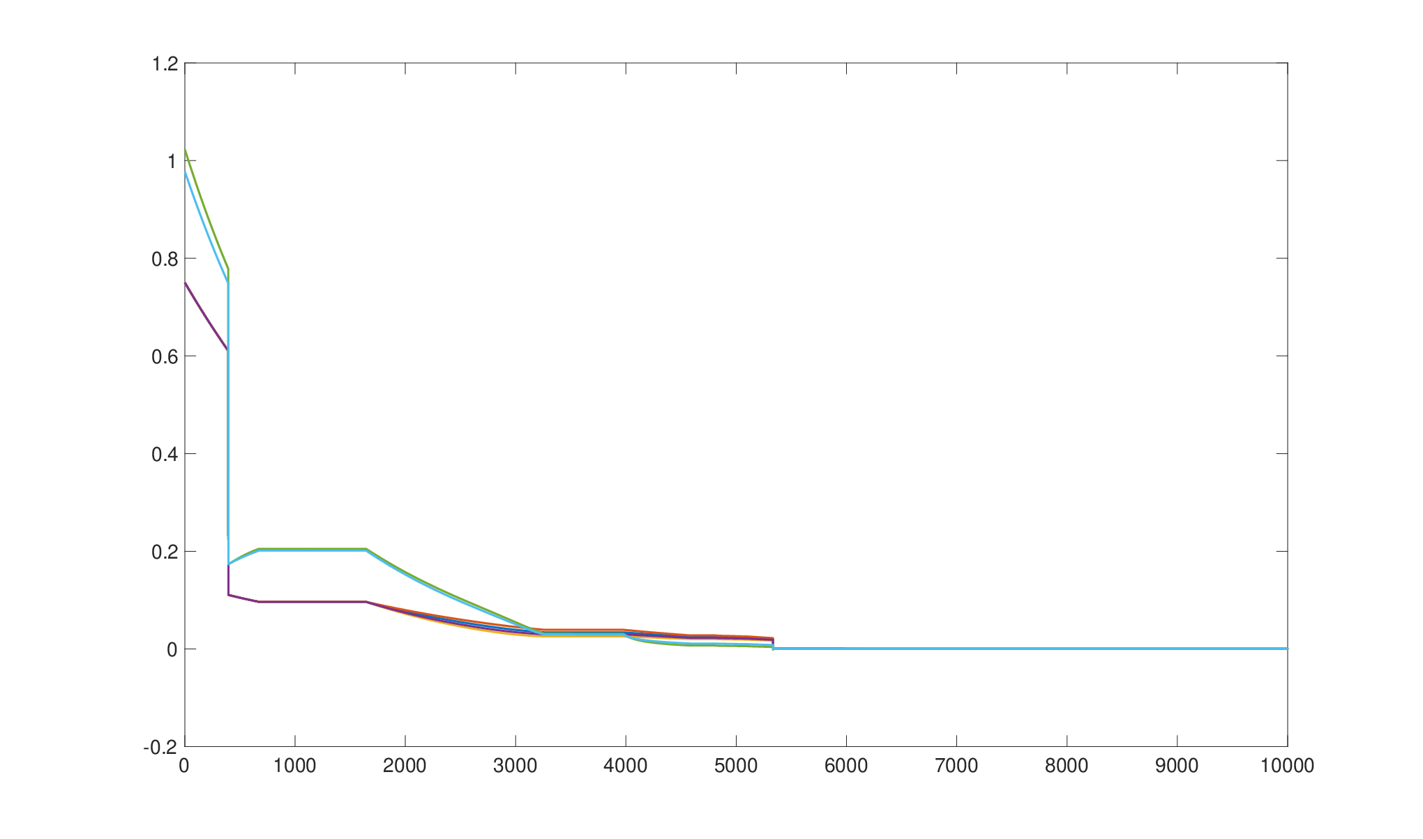
The next of them represent , whose evolution is shown in Figure 3.

The next of them represent , whose evolution is shown in Figure 4.

The final of them represent , whose evolution is shown in Figure 5.

As one can see, the outputs of converge to zero as expected.
Now let us look at the behavior of the mean-field term. It can be seen in Figure 6 that mean-field term converges to the following distribution . Hence, at the equilibrium, of the states are healthy.

If we also analyze the behavior of the equilibrium policy, it can be seen in Figure 7 and Figure 8 that equilibrium policy converges to the following conditional distribution and . Hence, once an agent is infected, then with probability , it should apply repair action. However, if the agent is healthy, then it should do nothing with probability . This is probably because of the fact that the cost of repair is more expensive than the risk of infection.


6 Conclusion
In this paper we have introduced linear mean-field games, in which the interaction between agents is determined by the empirical distribution of their states. Using the mean-field approach, we have demonstrated the existence of approximate Nash equilibria for finite-population games when the number of agents is sufficiently large. Under mild technical conditions, it can be shown that the limiting mean-field problem has an equilibrium. We have then applied the policy obtained from this equilibrium to the finite population game and proved that it constitutes an -Nash equilibrium for games with -agents, where an explicit relation between and has been established. Then, we have used linear programming and the linearity of transition probabilities in the mean-field term to convert the game into a generalized Nash equilibrium problem in the limit of an infinite number of agents. We have also developed an algorithm for finding a mean-field equilibrium with a guarantee of convergence.
References
- [1] [author] Adlakha, S.S., Johari, R.R. and Weintraub, G. Y.G. Y. (2015). Equilibria of dynamic games with many players: Existence, approximation, and market structure. Journal of Economic Theory 156 269–316.
- [2] [author] Anahtarci, BerkayB., Kariksiz, Can DehaC. D. and Saldi, NaciN. (2020). Value iteration algorithm for mean-field games. Systems and Control Letters 143 104744.
- [3] [author] Anahtarci, BerkayB., Kariksiz, Can DehaC. D. and Saldi, NaciN. (2022). Q-Learning in Regularized Mean-field Games. Dyn Games Appl.
- [4] [author] Bapat, R. B.R. B. and Raghavan, T. E. S.T. E. S. (1997). Nonnegative Matrices and Applications. Encyclopedia of Mathematics and its Applications. Cambridge University Press.
- [5] Basar, T. (2018). A Consensus Problem in Mean Field Setting with Noisy Measurements of Target. In 2018 Annual American Control Conference (ACC) 6521-6526.
- [6] [author] Bensoussan, A.A., Frehse, J.J. and Yam, P.P. (2013). Mean Field Games and Mean Field Type Control Theory. Springer, New York.
- [7] [author] Cardaliaguet, P.P. (2011). Notes on mean-field games.
- [8] [author] Carmona, R.R. and Delarue, F.F. (2013). Probabilistic analysis of mean-field games. SIAM J. Control Optim. 51 2705–2734.
- [9] [author] Dreves, AxelA., Facchinei, FranciscoF., Kanzow, ChristianC. and Sagratella, SimoneS. (2011). On the solution of the KKT conditions of generalized Nash equilibrium problems. SIAM Journal on Optimization 21 1082-1108.
- [10] [author] Dudley, R. M.R. M. (2004). Real Analysis and Probability. Cambridge University Press.
- [11] [author] Elliot, R.R., Li, X.X. and Ni, Y.Y. (2013). Discrete time mean-field stochastic linear-quadratic optimal control problems. Automatica 49 3222–3233.
- [12] [author] Facchinei, F.F. and Kanzow, ChristianC. (2010). Generalized Nash equilibrium problems. Annals of Operations Research 175 177-211.
- [13] [author] Facchinei, FranciscoF. and Pang, Jong-ShiJ.-S. (2003). Finite-dimensional variational inequalities and complementarity problems. Springer.
- [14] [author] Fournier, NicolasN. and Guillin, ArnaudA. (2015). On the rate of convergence in Wasserstein distance of the empirical measure. Probability Theory and Related Fields 162 707–738.
- [15] [author] Gomes, D. A.D. A., Mohr, J.J. and Souza, R. R.R. R. (2010). Discrete time, finite state space mean field games. J. Math. Pures Appl. 93 308–328.
- [16] [author] Gomes, D. A.D. A. and Saúde, J.J. (2014). Mean field games models - a brief survey. Dyn. Games Appl. 4 110–154.
- [17] [author] Gottlieb, Lee-AdL.-A., Kontorovich, AryehA. and Krauthgamer, RobertR. (2016). Adaptive metric dimensionality reduction. Theoretical Computer Science 620 105-118.
- [18] [author] Gottlieb, Lee-AdL.-A., Kontorovich, AryehA. and Krauthgamer, RobertR. (2017). Efficient Regression in Metric Spaces via Approximate Lipschitz Extension. IEEE Transactions on Information Theory 63 4838-4849.
- [19] [author] Hernandez-Lerma, O.O. and Gonzalez-Hernandez, J.J. (2000). Constrained Markov control processes in Borel spaces:the discounted case. Math. Meth. Oper. Res. 52 271–285.
- [20] [author] Hernández-Lerma, O.O. and Lasserre, J. B.J. B. (1996). Discrete-Time Markov Control Processes: Basic Optimality Criteria. Springer.
- [21] [author] Huang, M.M. (2010). Large-population LQG games involving major player: The Nash certainity equivalence principle. SIAM J. Control Optim. 48 3318–3353.
- [22] [author] Huang, M.M., Caines, P. E.P. E. and Malhamé, R. P.R. P. (2007). Large-population cost coupled LQG problems with nonuniform agents: Individual-mass behavior and decentralized -Nash equilibria. IEEE. Trans. Autom. Control 52 1560–1571.
- [23] [author] Huang, MinyiM. and Ma, YanY. (2019). Binary Mean Field Stochastic Games: Stationary Equilibria and Comparative Statics. Modeling, Stochastic Control, Optimization, and Applications.
- [24] [author] Huang, M.M., Malhamé, R. P.R. P. and Caines, P. E.P. E. (2006). Large population stochastic dynamic games: Closed loop McKean-Vlasov sysyems and the Nash certainity equivalence principle. Communications in Information Systems 6 221–252.
- [25] [author] Lasry, J.J. and Lions, P.P. (2007). Mean field games. Japan. J. Math. 2 229–260.
- [26] [author] Light, BarB. and Weintraub, Gabriel Y.G. Y. (2022). Mean Field Equilibrium: Uniqueness, Existence, and Comparative Statics. Operations Research 70 585-605.
- [27] [author] Monteiro, Renato D. C.R. D. C. and Pang, Jong-ShiJ.-S. (1999). A Potential Reduction Newton Method for Constrained Equations. SIAM Journal on Optimization 9 729-754.
- [28] Moon, J. and Basar, T. (2015). Discrete-time decentralized control using the risk-sensitive performance criterion in the large population regime: a mean field approach. In ACC 2015.
- [29] [author] Moon, J.J. and Basar, T.T. (2016). Robust mean field games for coupled Markov jump linear systems. International Journal of Control 89 1367-1381.
- [30] Moon, J. and Basar, T. (2016). Discrete-time mean field Stackelberg games with a large number of followers. In CDC 2016.
- [31] [author] Moon, JunJ. and Basar, TamerT. (2018). Linear quadratic mean field Stackelberg differential games. Automatica 97 200-213.
- [32] [author] Moon, JunJ. and Basar, TamerT. (2019). Risk-Sensitive Mean Field Games via the Stochastic Maximum Principle. Dynamic Games and Applications 1-26.
- [33] Nourian, M. and Nair, G. N. (2013). Linear-quadratic-Gaussian mean field games under high rate quantization. In CDC 2013.
- [34] [author] Saldi, NaciN., Basar, TamerT. and Raginsky, MaximM. (2018). Markov–Nash Equilibria in Mean-Field Games with Discounted Cost. SIAM Journal on Control and Optimization 56 4256-4287.
- [35] [author] Saldi, NaciN., Yüksel, SerdarS. and Linder, TamásT. (2017). On the Asymptotic Optimality of Finite Approximations to Markov Decision Processes with Borel Spaces. Mathematics of Operations Research 42 945-978.
- [36] Subramanian, J. and Mahajan, A. (2019). Reinforcement Learning in Stationary Mean-Field Games. 251-259. International Foundation for Autonomous Agents and Multiagent Systems.
- [37] [author] Tembine, H.H., Zhu, Q.Q. and Basar, T.T. (2014). Risk-sensitive mean field games. IEEE. Trans. Autom. Control 59 835–850.
- [38] [author] Villani, C.C. (2009). Optimal transport: Old and New. Springer.
- [39] [author] Weintraub, G. Y.G. Y., Benkard, C. L.C. L. and Roy, B. VanB. V. (2008). Markov perfect industry dynamics with many firms. Econometrica 76 1375–1411.
- [40] Weintraub, G., Benkard, L. and Van Roy, B. (2005). Oblivious Equilibrium: A Mean Field Approximation for Large-Scale Dynamic Games. In Advances in Neural Information Processing System.
- [41] [author] Weintraub, Gabriel Y.G. Y., Benkard, C. LanierC. L. and Van Roy, BenjaminB. (2010). Computational Methods for Oblivious Equilibrium. Operations Research 58 1247-1265.