Hybrid Parametric Classes of Isotropic Covariance Functions for Spatial Random Fields

In this study, we propose new parametric classes of isotropic covariance functions, $\widetilde{\varphi}(\cdot;\bm{\lambda},\bm{\omega},\bm{\xi})$, determined according to

where $g_{1}$ and $g_{2}$ are nonnegative functions on $[0,\xi_{1})$ and $[\xi_{2},\infty)$, respectively, and $\bm{\lambda}=[\bm{\lambda}_{1}^{\top},\bm{\lambda}_{2}^{\top}]^{\top}$, $\bm{\omega}=[\omega_{1},\omega_{2}]^{\top}$ and $\bm{\xi}=[\xi_{1},\xi_{2}]^{\top}$ are vectors of parameters, with $\omega_{i},\xi_{i}>0$, for $i=1,2$. In other words, we replace the mixing function, $g$, in Equation (2.1) with a function $\widetilde{g}$ that is defined piecewise, i.e.,

with $1_{A}(\cdot)$ standing for the indicator function of a set $A$. Note that $\widetilde{g}$ may have discontinuities as it is built by gluing two individual pieces. If the functions $g_{i}$ are continuous and bounded on their domains, a direct application of the dominated convergence theorem implies that the proposed covariance function (3.1) is continuous on $[0,\infty)$. Throughout this manuscript, each function $g_{i}$ is positively proportional to a continuous probability density function. Hence, the parametric family proposed in Equation (3.1) belongs to the Schoenberg class as defined through Equation (2.1).

A more general construction considers different kernels in each segment of the mixture, i.e.,

where $\bm{\vartheta}=[\bm{\vartheta}^{\top}_{1},\bm{\vartheta}^{\top}_{2}]^{\top}$. If $\phi_{i}$ is a valid covariance function in $\mathbb{R}^{d}$ for $d\leq d^{\prime}_{i}$, for some $d_{i}^{\prime}\in\mathbb{N}$, $i=1,2$, then (3.3) is a valid model in $\mathbb{R}^{d}$ if and only if $d\leq\text{min}(d^{\prime}_{1},d^{\prime}_{2})$. The continuity of (3.3) can be justified by following the same arguments used for the continuity of (3.1).

The apparent flexibility of the proposed mixtures is justified by classical theory on local and global behaviour of covariance functions. In particular, a direct application of Tauberian theorems (Stein, 1999) proves that mean square differentiability of $\widetilde{\varphi}$ will be determined by $g_{2}$. On the other hand, direct inspection in concert with Equation (4) in Gneiting and Schlather, 2004 shows that the long term behaviour of $\widetilde{\varphi}$ is decided by $g_{1}$. The next sections show that it is possible to provide examples in algebraically closed form that allow to attain the desired flexibility.

We present a hybrid Cauchy-Matérn model, for which the acronym ${\cal CM}$ is used. This model is a special case of (3.1). Let us first introduce the generalized incomplete gamma function (Chaudhry and Zubair, 1994),

and the lower incomplete gamma function, $\gamma(a,b)=\Gamma(a;0;0)-\Gamma(a;b;0)$.

When $\nu_{2}=n+1/2$, for some $n\in\mathbb{N}$, (3.6) can be expressed in terms of complementary error functions and modified Bessel functions of first and second kinds. We refer the reader to Alegría et al., 2021 for a more detailed study of these special cases.

The flexibility of the proposed structure is now illustrated through the following result, where we use the notation $f_{1}(h)\sim f_{2}(h)$, $h\rightarrow\infty$, to represent that, for some positive constant $c_{0}$, the asymptotic relationship $\lim_{h\rightarrow\infty}f_{1}(h)/f_{2}(h)=c_{0}$ holds.

To wrap up, the hybrid Cauchy-Matérn model allows to index both mean square differentiability and long term behaviour of the associated Gaussian random field. We also note that these properties are independently addressed by the two parameters $\nu_{1}$ and $\nu_{2}$, and hence those parameters are statistically identifiable and allow to decouple local and global properties.

From a statistical viewpoint, a parsimonious choice may be considered by setting $\omega_{1}=\omega_{2}=\omega$, $\alpha_{1}=\alpha_{2}=\alpha$ and $\xi_{1}=\xi_{2}=\xi$. Thus, we obtain that Proposition 3.1 provides a five parameter family where $\omega$ indexes the variance, $\alpha$ the scale, $\nu_{2}$ the mean square differentiability, and $\nu_{1}$ the Hurst effect, whereas $\xi$ is a parameter that balances the shapes of the marginal structures involved in this model. Hence, (3.4) generalizes the Matérn model in that it allows for polynomial decay while indexing continuously mean square differentiability.

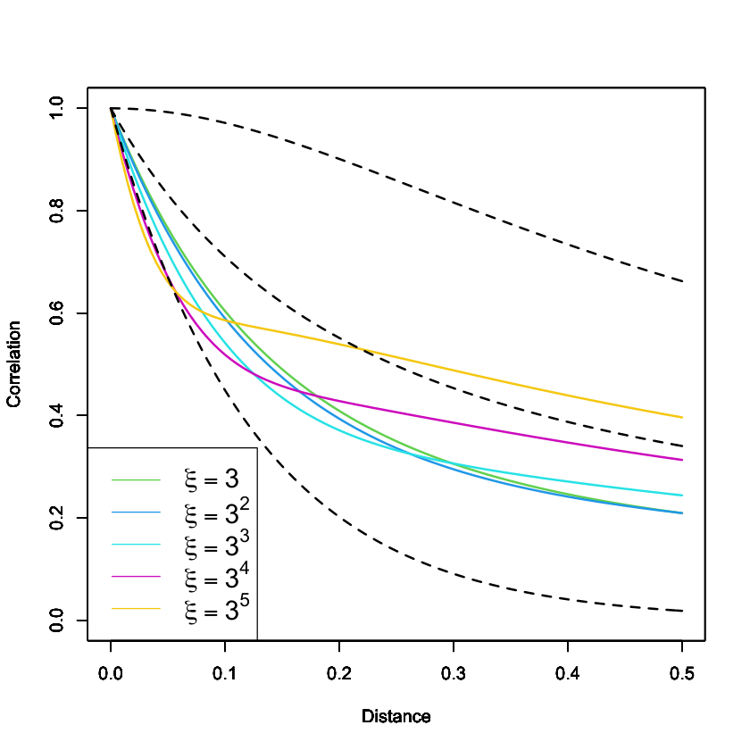
Figure 3.1 shows the parsimonious hybrid Cauchy-Matérn model for different values of $\xi$. The traditional Matérn and traditional Cauchy, as well as their average, which are also special cases of the hybrid construction, are reported for comparison purposes. Note that the curves have a linear or parabolic decay near the origin according to $\nu_{2}=1/2$ or $\nu_{2}=3/2$, respectively, and then the decay is more gradual (polynomial rate) for large distances according to $\nu_{1}$, which is consistent with the local and global patterns that are coexisting. We observe that $\xi$ has a manifest impact on the shape of the covariance function, as it produces some interesting forms (apparent changes of concavity) that could be useful in practice.

We now present a hybrid class of covariance functions, with local attributes of Matérn type, attaining negative values at large distances. We use the acronym $\mathcal{HM}$ for this model, termed hybrid Hole-Effect-Matérn. The proposed class comes from the mixture (3.3), where $\phi_{1}$ is chosen in such a way that the resulting model can take negative values.

The covariance function (3.14) always takes negative values (Posa, 2022), so it is a natural building block to achieve hybrid models with hole effect. The parameters in $\bm{\vartheta}$ are responsible for the sharpness of the hole effect. More precisely, as $\eta$ approaches $\tau^{2/d}$, the hole effect is more pronounced because the positive term in the right hand size of (3.14) has less dominance. Moreover, when $d=1$, we have the least restrictive condition on $\eta$, and the resulting hole effect is more marked. It is well known that the possibility of significant negative correlations vanishes as the dimension increases (see, e.g., page 45 in Stein, 1999).

The next proposition characterizes the local attributes of (3.11) and provides a lower bound for this model.

Note that as $\xi_{1}\rightarrow\infty$ (i.e., as the hole effect predominates), the lower bound in Equation (3.16) decreases to $(\tau\eta)^{-1/(\eta-1)}(1-\eta)/\eta$. On the contrary, as $\xi_{1}\rightarrow 0$, such a bound increases to zero, i.e., the hole effect becomes negligible, which is not surprising, because in such a case the Matérn class is predominant. A similar conclusion can be obtained in the limit case $\eta\rightarrow 1$.

A parsimonious variant of this model consists of taking $\omega_{1}=\omega_{2}=\omega$ (variance parameter), $\alpha_{1}=\alpha_{2}=\alpha$ (scale parameter) and $\nu_{1}=\nu_{2}=\nu$ (smoothness parameter), whereas $\bm{\vartheta}$ regulates the hole effect (as discussed above) and $\xi_{1}=\xi_{2}=\xi$ has a similar interpretation as in the hybrid Cauchy-Matérn model.

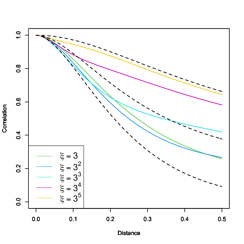
Figure 3.2 shows the parsimonious hybrid Hole-Effect-Matérn model for different values of $\xi$. The limit cases described in Remark 3.1 are also reported, in a similar fashion to Figure 3.1. It can be seen that negative values coexist with different levels of smoothness at the origin, as expected.

We conduct simulation studies to assess the performance of maximum likelihood inference when a hybrid covariance structure is present. We focus on the parsimonious hybrid Cauchy-Matérn dependence structure, as it will be applied to real data in the next section. We consider $\omega=1$, $\alpha=1/8$, $\nu_{1}=3/4$ and the following scenarios for $[\nu_{2},\xi]$: (a) $[1/2,40]$, (b) $[1/2,120]$, (c) $[3/2,40]$ and (d) $[3/2,120]$. For each scenario, we simulate 200 independent realizations of a Gaussian random field on 100 uniformly sampled points in the square $[0,3]^{2}$ and estimate the parameters through maximum likelihood. We then repeat the experiment with 256 spatial locations. We only estimate $\omega$ , $\alpha$ and $\xi$, whereas $\nu_{1}$ and $\nu_{2}$ are fixed, which is a common practice in geostatistics. Instead of directly estimating $\xi$, we consider the following alternative parameterization: $\widetilde{\xi}=\sqrt{\xi}\alpha$, which seems to be a natural choice according to Equations (3.5) and (3.6).

Figure 4.1 displays the results. The estimates are approximately unbiased and the variance decreases as the sample size increases from 100 to 256, which is an expected behaviour. The variability of the estimates substantially decreases in scenarios (c) and (d), i.e., when the random field is smoother, which is a typical attribute of likelihood-based estimates in this context (Bevilacqua and Gaetan, 2015). On the contrary, such a variability deteriorates as $\xi$ increases from $40$ to $120$. Figure 4.2 shows the log-likelihood in terms of $\xi$ and $\alpha$, with fixed $\omega$, for a single realization of the random field, under scenario (b). Although the surface has a clear maximum value, the objective function is apparently more flat in the direction of $\xi$. This could explain the increased variability in scenarios (b) and (d), with respect to (a) and (c). Despite the previous remarks, in general, the estimates appear to be reasonable in each scenario and no identifiability issues are observed.

We now explore the predictive performance of the proposed class through a cross validation analysis. We simulate 200 independent realizations on 100 uniformly sampled locations in $[0,3]^{2}$ according to the scenarios (a)-(d) described above. We assess the accuracy through a leave-one-out prediction strategy in terms of the mean squared error (MSE), mean absolute error (MAE), log-score (LSCORE) and continuous ranked probability score (CRPS) (see Zhang and Wang, 2010). Small values of these indicators suggest superior predictions. We evaluate the performance of the hybrid Cauchy-Matérn model, using the Generalized Cauchy class as benchmark. Thus, for each realization, we estimate the parameters with both models and proceed to make the predictions through a simple kriging approach. The Generalized Cauchy model (2.4) has been augmented with a multiplicative parameter $\omega$, namely $h\mapsto\omega(1+h^{\delta}/\alpha)^{-\nu/\delta}$, so it is parameterized by $\omega$ and ${\alpha}$, and $\nu=3/4$ and $\delta=1,2$ are fixed.

Table 4.1 shows that, in each scenario, the proposed hybrid model outperforms its competitor. All the cross-validation scores substantially decrease in scenarios (c) and (d). From this brief study, we observe that when the true underlying covariance has a hybrid structure, an incorrect specification of the spatial association has a negative impact on the posterior predictions. Since the behaviour of an isotropic covariance function near the origin has a strong impact on the quality of predictions (Stein, 1999), our simulation experiment suggests that in some circumstances the local shape of the proposed model cannot be replicated by other appealing existing structures.

The estimation of recoverable resources is a task of fundamental importance in modern mining processes. A sound evaluation of such resources is crucial from an economic viewpoint and is critical for assessing the long-term availability of mineral resources and its impact on society. We consider a data set from a lateritic nickel deposit mined by open pit in Colombia, which contains measurements of the grades of nickel, iron, chrome, alumina, magnesia and silica.

This study focuses on nickel concentrations that are placed at an elevation of about $120$ meters, where $199$ irregularly spaced observations are available. We apply a log-transformation to reduce the skewness, and then the sample mean is subtracted. The resulting values are approximately Gaussian. The left panel of Figure 4.4 shows the transformed data set. We fit two covariance models: the former is the parsimonious hybrid Cauchy-Matérn, parameterized by $\omega$, ${\alpha}$ and $\widetilde{\xi}$, with fixed $\nu_{1}=1/4$ and $\nu_{2}=1/2$, and the latter is the Generalized Cauchy, parameterized as in Section 4.1, with fixed $\nu=1/4$ and $\delta=0.95$. The values of the fixed parameters have been selected after some experimental trials, taking into account the local behavior of the sample covariance (see Figure 4.3).

Table 4.2 reports the likelihood estimates, with the corresponding standard errors, and the Akaike information criterion (AIC). We observe that the hybrid Cauchy-Matérn model outperforms its competitor in terms of AIC. Figure 4.3 shows that the fitted covariance models seem to be reasonably close to the sample covariance. The fitted models differ substantially near the origin (distances less than 3 meters), since the hybrid model decays faster. On the contrary, for larger distances the hybrid model decays slower, although the difference between the curves becomes slight for distances greater than $15$ meters.

In order to compare the models in terms of predictive performance, we conduct a cross-validation study, in a similar fashion to the experiments performed with simulated data. Table 4.3 shows evidence, based on a leave-one-out cross-validation scheme, that the hybrid model has a better performance for this specific data set. In percentage terms, the MSE shows an improvement of approximately $3.4\%$. The largest difference occurs when we compare the LSCORE’s (about $9\%$ improvement).

We conclude this section with an illustration of a downscaled map of log-nickel concentrations (see Figure 4.4), using the hybrid Cauchy-Matérn model. The interpolated spatial map, which is obtained through simple kriging, is exhibited on a spatial grid of approximately $1$ meter ($7500$ locations). This kriged surface could be useful in small-scale mining processes, as it is a crucial step for industrial exploration and to quantify mineral reserves.

In many practical situations, two or more variables are simultaneously recorded. Thus, our findings can be generalized to the case of multivariate fields $\{{\bf Z}({\bf s})=(Z_{1}({\bf s}),\ldots,Z_{p}({\bf s}))^{\top},\;{\bf s}\in\mathbb{R}^{d}\}$, having an isotropic matrix-valued covariance function $\Phi:[0,\infty)\to\mathbb{R}^{p\times p}$, that is, ${\rm cov}[Z_{i}({\bf s}),Z_{j}({\bf s}^{\prime})]=\Phi_{ij}(h)$, $h\geq 0$, where $h=\|{\bf s}-{\bf s}^{\prime}\|$ and $i,j=1,\ldots,p$. We propose the hybrid model

that generalizes (3.1), where the vectors of parameters $\bm{\lambda}_{i}$ must be chosen in such a way that the $p\times p$ matrices ${\bf G}_{i}(u;\bm{\lambda}_{i})$ are positive semi-definite for every fixed $u\geq 0$. Hence, a straight application of Proposition 4 in Porcu and Zastavnyi, 2011 would ensure $\widetilde{\Phi}$ to be positive semi-definite. A multivariate version of the hybrid Cauchy-Matérn covariance function is a natural candidate. The works of Gneiting et al., 2010 and Moreva and Schlather, 2022 are relevant to tackle this challenge. A multivariate version of the formulation (3.3) could be deduced similarly.

For random fields that are indexed by the $d$-dimensional unit sphere, $\mathbb{S}^{d}$, which is a useful framework when analyzing global data ($\mathbb{S}^{2}$ is used as an approximation of the Earth), the isotropy assumption is given by ${\rm cov}[Z({\bf s}),Z({\bf s}^{\prime})]=\psi(\theta)$, ${\bf s},{\bf s}^{\prime}\in\mathbb{S}^{d}$, where $\psi:[0,\pi]\rightarrow\mathbb{R}$ is a continuous mapping and $\theta=\arccos({\bf s}^{\top}{\bf s}^{\prime})\in[0,\pi]$ is the geodesic distance. Schoenberg’s characterization (Schoenberg, 1942) establishes that a parametric isotropic covariance function $\psi(;\bm{\lambda})$ is valid in any dimension $d$, if and only if, it can be written as ${\psi}(\theta;\bm{\lambda})=\sum_{\ell=0}^{\infty}\beta_{\ell}(\bm{\lambda})(\cos\theta)^{\ell}$, $\theta\in[0,\pi]$, for some nonnegative and summable parametric sequence $\{\beta_{\ell}(\bm{\lambda})\}_{\ell=0}^{\infty}$. Thus, the hybrid models can be adapted to the spherical context by considering a modified sequence of the form

where $\lfloor\xi_{i}\rfloor\geq 0$, for $i=1,2$, with $\lfloor\cdot\rfloor$ standing for the floor function, and $\beta_{\ell}^{(i)}$ being a nonnegative and summable sequence. The local properties of spherically indexed random fields, and their connections with the covariance function, have been studied in past literature (Bingham, 1973; Guinness and Fuentes, 2016). However, global properties such as long memory are less intuitive in this scenario as the spatial domain is a compact set. Covariance functions with hole effect, for low-dimensional spheres, could be obtained by adapting formulation (3.3).

References

- Abramowitz and Stegun, (1972) Abramowitz, M. and Stegun, I. A. (1972). Handbook of Mathematical Functions with Formulas, Graphs, and Mathematical Tables. Dover Publications.
- Alegría, (2020) Alegría, A. (2020). Cross-dimple in the cross-covariance functions of bivariate isotropic random fields on spheres. Stat, 9(1):e301.
- Alegría et al., (2021) Alegría, A., Emery, X., and Porcu, E. (2021). Bivariate Matérn covariances with cross-dimple for modeling coregionalized variables. Spatial Statistics, 41:100491.
- Barndorff-Nielsen, (1978) Barndorff-Nielsen, O. (1978). Hyperbolic distributions and distributions on hyperbolae. Scandinavian Journal of Statistics, 5(3):151–157.
- Barp et al., (2022) Barp, A., Oates, C. J., Porcu, E., and Girolami, M. (2022). A Riemann–Stein kernel method. Bernoulli, 28(4):2181–2208.
- Berg et al., (2008) Berg, C., Mateu, J., and Porcu, E. (2008). The Dagum family of isotropic correlation functions. Bernoulli, 14(4):1134–1149.
- Bevilacqua et al., (2022) Bevilacqua, M., Caamaño-Carrillo, C., and Porcu, E. (2022). Unifying compactly supported and Matérn covariance functions in spatial statistics. Journal of Multivariate Analysis, 189:104949.
- Bevilacqua and Gaetan, (2015) Bevilacqua, M. and Gaetan, C. (2015). Comparing composite likelihood methods based on pairs for spatial Gaussian random fields. Statistics and Computing, 25(5):877–892.
- Bingham, (1973) Bingham, N. H. (1973). Positive Definite Functions on Spheres. Proc. Cambridge Phil. Soc., 73:145–156.
- Chaudhry and Zubair, (1994) Chaudhry, M. A. and Zubair, S. M. (1994). Generalized incomplete gamma functions with applications. Journal of Computational and Applied Mathematics, 55(1):99–123.
- Chen et al., (2018) Chen, W., Castruccio, S., Genton, M. G., and Crippa, P. (2018). Current and future estimates of wind energy potential over Saudi Arabia. Journal of Geophysical Research: Atmospheres, 123(12):6443–6459.
- Chilès and Delfiner, (2012) Chilès, J.-P. and Delfiner, P. (2012). Geostatistics: Modeling Spatial Uncertainty, Second Edition. John Wiley & Sons.
- Cockayne et al., (2019) Cockayne, J., Oates, C. J., Sullivan, T. J., and Girolami, M. (2019). Bayesian probabilistic numerical methods. SIAM review, 61(4):756–789.
- Cressie, (1993) Cressie, N. (1993). Statistics for Spatial Data. Wiley, New York, revised edition.
- Cressie and Kornak, (2003) Cressie, N. and Kornak, J. (2003). Spatial Statistics in the Presence of Location Error with an Application to Remote Sensing of the Environment. Statistical Science, 18(4):436–456.
- Daley and Porcu, (2014) Daley, D. and Porcu, E. (2014). Dimension walks and Schoenberg spectral measures. Proceedings of the American Mathematical Society, 142(5):1813–1824.
- Di Lorenzo et al., (2014) Di Lorenzo, E., Combes, V., Keister, J., Strub, P., Andrew, T., Peter, F., Marck, O., Furtado, J. ., Bracco, A., Bograd, S., Peterson, W., Schwing, F., Taguchi, B., Hormázabal, S., and Parada, C. (2014). Synthesis of Pacific Ocean Climate and ecosystem dynamics. Oceanography, 26(4):68–81.
- Edwards et al., (2019) Edwards, M., Castruccio, S., and Hammerling, D. (2019). A multivariate Global Spatio-Temporal Stochastic Generator for Climate Ensembles. Journal of Agricultural, Biological and Environmental Sciences.
- Emery and Lantuéjoul, (2006) Emery, X. and Lantuéjoul, C. (2006). Tbsim: A computer program for conditional simulation of three-dimensional gaussian random fields via the turning bands method. Computers & Geosciences, 32(10):1615–1628.
- Emery and Séguret, (2020) Emery, X. and Séguret, S. A. (2020). Geostatistics for the Mining Industry: Applications to Porphyry Copper Deposits. CRC Press.
- Furrer et al., (2006) Furrer, R., Genton, M. G., and Nychka, D. (2006). Covariance tapering for interpolation of large spatial datasets. Journal of Computational and Graphical Statistics, 15(3):502–523.
- Furrer et al., (2007) Furrer, R., Sain, S. R., Nychka, D., and Meehl, G. A. (2007). Multivariate bayesian analysis of atmosphere–ocean general circulation models. Environmental and Ecological Statistics, 14(3):249–266.
- Gneiting et al., (2010) Gneiting, T., Kleiber, W., and Schlather, M. (2010). Matérn cross-covariance functions for multivariate random fields. Journal of the American Statistical Association, 105:1167–1177.
- Gneiting and Schlather, (2004) Gneiting, T. and Schlather, M. (2004). Stochastic models that separate fractal dimension and the Hurst effect. SIAM review, 46(2):269–282.
- Gradshteyn and Ryzhik, (2007) Gradshteyn, I. and Ryzhik, I. (2007). Table of Integrals, Series, and Products. Academic Press, Amsterdam, 7th. edition.
- Guinness and Fuentes, (2016) Guinness, J. and Fuentes, M. (2016). Isotropic covariance functions on spheres: Some properties and modeling considerations. Journal of Multivariate Analysis, 143:143–152.
- Guinness and Hammerling, (2018) Guinness, J. and Hammerling, D. (2018). Compression and conditional emulation of climate model output. Journal of the American Statistical Association, 113(521):56–67.
- Hristopulos, (2020) Hristopulos, D. T. (2020). Random fields for spatial data modeling. Springer.
- James et al., (2013) James, G., Witten, D., Hastie, T., and Tibshirani, R. (2013). An introduction to statistical learning, volume 112. Springer.
- Kaufman et al., (2008) Kaufman, C. G., Schervish, M. J., and Nychka, D. W. (2008). Covariance tapering for likelihood-based estimation in large spatial data sets. Journal of the American Statistical Association, 103(484):1545–1555.
- Laga and Kleiber, (2017) Laga, I. and Kleiber, W. (2017). The modified Matérn process. Stat, 6(1):241–247.
- Ma and Bhadra, (2022) Ma, P. and Bhadra, A. (2022). Beyond Matérn: On a Class of Interpretable Confluent Hypergeometric Covariance Functions. Journal of the American Statistical Association, (in press).
- Matérn, (1986) Matérn, B. (1986). Spatial Variation — Stochastic Models and Their Application to Some Problems in Forest Surveys and Other Sampling Investigations. Springer.
- Moreva and Schlather, (2022) Moreva, O. and Schlather, M. (2022). Bivariate covariance functions of Pólya type. Journal of Multivariate Analysis, in press.
- Ostoja-Starzewski, (2006) Ostoja-Starzewski, M. (2006). Material spatial randomness: From statistical to representative volume element. Probabilistic engineering mechanics, 21(2):112–132.
- Pazouki and Schaback, (2011) Pazouki, M. and Schaback, R. (2011). Bases for kernel-based spaces. Journal of Computational and Applied Mathematics, 236(4):575–588.
- (37) Porcu, E., Alegria, A., and Furrer, R. (2018a). Modeling temporally evolving and spatially globally dependent data. International Statistical Review, 86(2):344–377.
- (38) Porcu, E., Bevilacqua, M., and Hering, A. S. (2018b). The Shkarofsky-Gneiting class of covariance models for bivariate Gaussian random fields. Stat, 7(1):e207.
- Porcu and Zastavnyi, (2011) Porcu, E. and Zastavnyi, V. (2011). Characterization theorems for some classes of covariance functions associated to vector valued random fields. Journal of Multivariate Analysis, 102(9):1293–1301.
- Posa, (2022) Posa, D. (2022). Special classes of isotropic covariance functions. Preprint, Research Square.
- Schaback and Wendland, (2006) Schaback, R. and Wendland, H. (2006). Kernel techniques: from machine learning to meshless methods. Acta numerica, 15:543–639.
- Schlather, (2010) Schlather, M. (2010). Some covariance models based on normal scale mixtures. Bernoulli, 16(3):780–797.
- Schlather and Moreva, (2017) Schlather, M. and Moreva, O. (2017). A parametric model bridging between bounded and unbounded variograms. Stat, 6(1):47–52.
- Schoenberg, (1938) Schoenberg, I. J. (1938). Metric Spaces and Completely Monotone Functions. Annals of Mathematics, 39(4):811–841.
- Schoenberg, (1942) Schoenberg, I. J. (1942). Positive definite functions on spheres. Duke Mathematical Journal, 9(1):96–108.
- Stein, (1999) Stein, M. L. (1999). Statistical Interpolation of Spatial Data: Some Theory for Kriging. Springer, New York.
- Stein, (2007) Stein, M. L. (2007). Spatial variation of total column ozone on a global scale. The Annals of Applied Statistics, 1(1):191–210.
- Yaglom, (1987) Yaglom, A. M. (1987). Correlation Theory of Stationary and Related Random Functions, Volume I: Basic Results, volume 131. Springer.
- Zhang and Wang, (2010) Zhang, H. and Wang, Y. (2010). Kriging and cross-validation for massive spatial data. Environmetrics, 21(3-4):290–304.