Bivariate distributions on the unit square: Theoretical properties and applications

Roberto Vila Thanks: rovig161@gmail.com Affiliation: Department of Statistics, University of Brasília, Brasília, Brazil Affiliation: Department of Mathematics and Statistics, McMaster University, Hamilton, Ontario, Canada Narayanaswamy Balakrishnan Thanks: bala@mcmaster.ca Affiliation: Department of Mathematics and Statistics, McMaster University, Hamilton, Ontario, Canada Helton Saulo Thanks: heltonsaulo@gmail.com Affiliation: Department of Statistics, University of Brasília, Brasília, Brazil
Peter Zörnig Thanks: peter@unb.br Affiliation: Department of Statistics, University of Brasília, Brasília, Brazil

Abstract

We introduce the bivariate unit-log-symmetric model based on the bivariate log-symmetric distribution (BLS) defined in Vila et al., 2022 as a flexible family of bivariate distributions over the unit square. We then study its mathematical properties such as stochastic representations, quantiles, conditional distributions, independence of the marginal distributions and moments. Maximum likelihood estimation method is discussed and examined through Monte Carlo simulation. Finally, the proposed model is used to analyze soccer data.

Keywords. Bivariate unit-log-symmetric distribution $\cdot$ Bivariate log-symmetric distribution $\cdot$ Bivariate model $\cdot$ MCMC $\cdot$ Proportion data $\cdot$ Soccer data $\cdot$ Maximum likelihood estimation.
Mathematics Subject Classification (2010). MSC 60E05 $\cdot$ MSC 62Exx $\cdot$ MSC 62Fxx.

1 Introduction

Bivariate distributions over the unit-square have been discussed in detail in the literature. Many of them are based on beta distribution and its generalizations; see Arnold and Ng, 2011 and Nadarajah et al., 2017. Models of this type have been studied since the 1980s. Some other distributions on the unit square are based on generalized arcsine and inverse Gaussian distributions. A recent model, the bivariate unit-sinh-normal distribution, is based on the bivariate Birnbaum-Saunders distribution; see Martínez-Flórez et al., 2022. Bivariate distributions over the unit square arise naturally in comparing indices, rates or proportions in the interval $(0,1)$ .

In this paper, we study the bivariate unit-log-symmetric (BULS) distribution defined over the unit-square, obtained as a modification of the bivariate log-symmetric (BLS) distribution introduced by Vila et al., 2022. The definitions of BLS and BULS distributions are given in Section 2, along with some special cases of BULS. In Section 3, we discuss some properties of the new model, including a stochastic representation, marginal quantiles, and the conditional distributions of BULS. We derive more compact formulas for the conditional densities, using the distribution functions of normal, Student- $t$ , hyperbolic, Laplace and slash distributions. One of the uses of having closed formulas for the conditional densities (of the BULS model), for example, is in studying Heckman-type selection models (Heckman, 1979) when the selection variables have bounded support. In addition, we derive the distribution of the squared Mahalanobis distance of a random vector $\bm{W}=(W_{1},W_{2})^{\top}$ with BULS distribution, and present a necessary condition for the independence of the components of $\bm{W}$ and formulas for the moments of $W_{1}$ and $W_{2}$ . In Section 4, the log-likelihood function and the likelihood equations for the BULS distribution are presented. In Section 5, we carry out a Monte Carlo simulation study to evaluate the performance of the ML estimators by means of their bias, root mean square error and coverage probability. In Section 6, we present two applications to soccer data. Specifically, in Section 6.1, we model the vector $\bm{W}=(W_{1},W_{2})^{\top}$ , where $W_{1}$ represents the time elapsed until a first kick goal (of any team) and the time elapsed until a goal of any type of the home team, and show that specific BULS distributions are suitable for modelling $\bm{W}$ . In Section 6.2, we consider the data of 2022 FIFA World Cup wherein the components of the vector $\bm{W}$ represent the pass completion proportions of medium passes (14 to 18 meters) and long passes (longer than 37 meters). We then demonstrate that these data can also be fitted well by BULS distributions.

2 Bivariate unit-log-symmetric model

In this section, we describe the bivariate unit-log-symmetric model (BULS). To define this model, we first need to describe the bivariate log-symmetric distribution (BLS) defined in Vila et al., 2022.

2.1 BLS distribution

Following Vila et al., 2022, a continuous random vector $\bm{T}=(T_{1},T_{2})^{\top}$ is said to have a bivariate log-symmetric (BLS) distribution if its joint probability density function (PDF) is given by

\displaystyle f_{T_{1},T_{2}}(t_{1},t_{2};\bm{\theta})={1\over t_{1}t_{2}\sigma_{1}\sigma_{2}\sqrt{1-\rho^{2}}Z_{g_{c}}}\,g_{c}\Biggl({\widetilde{t_{1}}^{2}-2\rho\widetilde{t_{1}}\widetilde{t_{2}}+\widetilde{t_{2}}^{2}\over 1-\rho^{2}}\Biggr),\quad t_{1},t_{2}>0,

(2.1)

where $\widetilde{t_{i}}=\log[({t_{i}/\eta_{i}})^{1/\sigma_{i}}],\ \eta_{i}=\exp(\mu_{i}),\ i=1,2$ , with $\bm{\theta}=(\eta_{1},\eta_{2},\sigma_{1},\sigma_{2},\rho)^{\top}$ being the parameter vector, $\mu_{i}\in\mathbb{R}$ , $\sigma_{i}>0$ , $i=1,2$ and $\rho\in(-1,1)$ . Furthermore, $Z_{g_{c}}>0$ is the partition function, that is,

\displaystyle Z_{g_{c}}

\displaystyle=\int_{0}^{\infty}\int_{0}^{\infty}{1\over t_{1}t_{2}\sigma_{1}\sigma_{2}\sqrt{1-\rho^{2}}}\,g_{c}\Biggl({\widetilde{t_{1}}^{2}-2\rho\widetilde{t_{1}}\widetilde{t_{2}}+\widetilde{t_{2}}^{2}\over 1-\rho^{2}}\Biggr)\,{\rm d}t_{1}{\rm d}t_{2}=\pi\int_{0}^{\infty}g_{c}(u)\,{\rm d}u,

(2.2)

and $g_{c}$ is a scalar function referred to as the density generator (Fang et al., 1990, see). The second integral in (2.2) is consequence of a change of variables; for more details, see Proposition 3.1 of Vila et al., 2022. When a random vector $\bm{T}$ is BLS distributed, with parameter vector $\bm{\theta}$ , we denote it by $\bm{T}\sim{\rm BLS}(\bm{\theta},g_{c})$ .

2.2 BULS distribution

We say that a continuous random vector $\bm{W}=(W_{1},W_{2})^{\top}$ has a bivariate unit-log-symmetric (BULS) distribution with parameter vector $\bm{\theta}=(\eta_{1},\eta_{2},\sigma_{1},\sigma_{2},\rho)^{\top}$ , denoted by $\bm{W}\sim{\rm BULS}(\bm{\theta},g_{c})$ , if its PDF is, for $0<w_{1},w_{2}<1$ , given by

\displaystyle f_{W_{1},W_{2}}(w_{1},w_{2};\bm{\theta})={1\over(1-w_{1})t_{1}\sigma_{1}(1-w_{2})t_{2}\sigma_{2}\sqrt{1-\rho^{2}}Z_{g_{c}}}\,{\displaystyle g_{c}\Biggl({\widetilde{w}_{1}^{2}-2\rho\widetilde{w}_{1}\widetilde{w}_{2}+\widetilde{w}_{2}^{2}\over 1-\rho^{2}}\Biggr)},

(2.3)

where $\widetilde{w}_{i}=\log[({t_{i}/\eta_{i}})^{1/\sigma_{i}}],\ t_{i}=-\log(1-w_{i}),\ \eta_{i}=\exp(\mu_{i}),\ i=1,2$ , with $\sigma_{i}>0$ , $i=1,2$ , $\rho\in(-1,1)$ , and $Z_{g_{c}}$ and ${g_{c}}$ are as given in (2.2). We shall prove later that the BULS PDF in (2.3) is obtained by taking $W_{i}=1-\exp(-T_{i})$ , $i=1,2$ , with $=(T_{1},T_{2})^{\top}\sim{\rm BLS}(\bm{\theta},g_{c})$ .

Table 1 presents some examples of bivariate unit-log-symmetric distributions.

Table 1: Partition functions

(Z_{g_{c}})

and density generators

(g_{c})

for some BULS distributions.

Distribution	$Z_{g_{c}}$	$g_{c}$	Parameter
Bivariate unit-log-normal	$2\pi$	$\exp(-x/2)$	$-$
Bivariate unit-log-Student- $t$	${{\Gamma({\nu/2})}\nu\pi\over{\Gamma({(\nu+2)/2})}}$	$(1+{x\over\nu})^{-(\nu+2)/2}$	$\nu>0$
Bivariate unit-log-hyperbolic	${2\pi(\nu+1)\exp(-\nu)\over\nu^{2}}$	$\exp(-\nu\sqrt{1+x})$	$\nu>0$
Bivariate unit-log-Laplace	$\pi$	$K_{0}(\sqrt{2x})$	$-$
Bivariate unit-log-slash	${\pi\over q}\,2^{2-q\over 2}$	$x^{-{q+2\over 2}}\gamma({q+2\over 2},{x\over 2})$	$q>0$

In Table 1, $\Gamma(t)=\int_{0}^{\infty}x^{t-1}\exp(-x)\,{\rm d}x$ , $t>0$ , is the complete gamma function, $K_{\lambda}(u)=(1/2)(u/2)^{\lambda}\int_{0}^{\infty}t^{-\lambda-1}\exp(-t-{u^{2}/4t})\,{\rm d}t$ , $u>0$ , is the modified Bessel function of the third kind with index $\lambda$ (Kotz et al., 2001, see Appendix of ), and $\gamma(s,x)=\int_{0}^{x}t^{s-1}\exp(-t)\,{\rm d}t$ is the lower incomplete gamma function.

Let $\bm{T}=(T_{1},T_{2})^{\top}\sim{\rm BLS}(\bm{\theta},g_{c})$ . From (2.3), it is clear that the random vector $\bm{X}=(X_{1},X_{2})^{\top}$ , with

\displaystyle X_{i}=\log(T_{i})=\log\big[-\log(1-W_{i})\big],\quad i=1,2,

(2.4)

has a bivariate elliptically symmetric (BSY) distribution (Balakrishnan and Lai, 2009, see p. 592 in); that is, the PDF of $\bm{X}$ is

\displaystyle f_{X_{1},X_{2}}(x_{1},x_{2};\bm{\theta}_{*})={1\over\sigma_{1}\sigma_{2}\sqrt{1-\rho^{2}}Z_{g_{c}}}\,g_{c}\Biggl({\widetilde{x_{1}}^{2}-2\rho\widetilde{x_{1}}\widetilde{x_{2}}+\widetilde{x_{2}}^{2}\over 1-\rho^{2}}\Biggr),\quad-\infty<x_{1},x_{2}<\infty,

(2.5)

where $\widetilde{x_{i}}={(x_{i}-\mu_{i})/\sigma_{i}},\ i=1,2$ , with $\bm{\theta}_{*}=(\mu_{1},\mu_{2},\sigma_{1},\sigma_{2},\rho)$ being the parameter vector and $Z_{g_{c}}$ is the partition function defined in (2.2). In this case, we shall use the notation $\bm{X}\sim{\rm BSY}(\bm{\theta}_{*},g_{c})$ .

It is a simple task to observe that the joint cumulative distribution function (CDF) of $\bm{W}\sim{\rm BULS}(\bm{\theta},g_{c})$ , denoted by $F_{W_{1},W_{2}}(w_{1},w_{2};\bm{\theta})$ , is given by

	$\displaystyle F_{W_{1},W_{2}}(w_{1},w_{2};\bm{\theta})$	$\displaystyle=F_{T_{1},T_{2}}\big(-\log(1-w_{1}),-\log(1-w_{2});\bm{\theta}\big)$
		$\displaystyle=F_{X_{1},X_{2}}\big(\log[-\log(1-w_{1})],\log[-\log(1-w_{2})];\bm{\theta}_{*}\big),$

wherein $F_{T_{1},T_{2}}(t_{1},t_{2};\bm{\theta})$ and $F_{X_{1},X_{2}}(x_{1},x_{2};\bm{\theta}_{*})$ denote the CDFs of $\bm{T}\sim{\rm BLS}(\bm{\theta},g_{c})$ and $\bm{X}\sim{\rm BES}(\bm{\theta}_{*},g_{c})$ , respectively. Note that there is no closed form expression for the CDF of $\bm{X}$ with the exception of bivariate normal.

3 Some basic properties of the model

In this section, some mathematical properties of the bivariate unit-log-symmetric distribution are established.

3.1 Stochastic representation

Proposition 3.1.

The random vector $\bm{W}=(W_{1},W_{2})^{\top}$ has a BULS distribution if

\displaystyle\begin{array}[]{lllll}&W_{1}=1-\exp\big[-\eta_{1}\exp(\sigma_{1}Z_{1})\big],\\[11.38092pt] &W_{2}=1-\exp\big[-\eta_{2}\exp\big(\sigma_{2}{\rho}Z_{1}+\sigma_{2}\sqrt{1-\rho^{2}}Z_{2}\big)\big],\end{array}

where $Z_{1}=RDU_{1}$ and $Z_{2}=R\sqrt{1-D^{2}}U_{2}$ with $U_{1}$ , $U_{2}$ , $R$ , and $D$ being mutually independent random variables, $\rho\in(-1,1)$ , $\eta_{i}=\exp(\mu_{i})$ , and $\mathbb{P}(U_{i}=-1)=\mathbb{P}(U_{i}=1)=1/2$ , $i=1,2$ . The random variable $D$ is positive and has PDF $f_{D}(d)={2/(\pi\sqrt{1-d^{2}})},\ d\in(0,1).$ Further, the positive random variable $R$ has its PDF as $f_{R}(r)={2rg_{c}(r^{2})/\int_{0}^{\infty}g_{c}(u)\,{\rm d}{u}},\ r>0.$

Proof.

It is well-known that (Vila et al., 2022, see Proposition 3.2 of) the random vector $\bm{T}=(T_{1},T_{2})^{\top}$ has a BLS distribution if

\displaystyle\begin{array}[]{lllll}&T_{1}=\eta_{1}\exp(\sigma_{1}Z_{1}),\\[11.38092pt] &T_{2}=\eta_{2}\exp\big(\sigma_{2}{\rho}Z_{1}+\sigma_{2}\sqrt{1-\rho^{2}}Z_{2}\big).\end{array}

Moreover, from (2.4), $W_{i}=1-\exp(-T_{i})$ , $i=1,2$ . Hence, the result. ∎

The following lemma provides a slight simplification in the representation of Proposition 3.1. This result plays a fundamental role in the next subsections, since all the probabilistic characteristics that depend on the distribution of $\rho Z_{1}+\sqrt{1-\rho^{2}}Z_{2}$ will be simplified since it has the same distribution as $Z_{2}$ .

Lemma 3.2.

For a Borelian subset $B$ of $(0,1)$ , we have

\displaystyle\mathbb{P}\left(\rho Z_{1}+\sqrt{1-\rho^{2}}Z_{2}\in{B}\right)=\mathbb{P}(Z_{2}\in B).

In other words, $\rho Z_{1}+\sqrt{1-\rho^{2}}Z_{2}$ and $Z_{2}$ have the same distribution.

Proof.

It is clear that the density of $\rho Z_{1}+\sqrt{1-\rho^{2}}{Z_{2}}$ is related to the joint density $f_{Z_{1},Z_{2}}$ by

\displaystyle f_{\rho Z_{1}+\sqrt{1-\rho^{2}}{Z_{2}}}(s_{2})={1\over\sqrt{1-\rho^{2}}}\int_{-\infty}^{\infty}f_{Z_{1},Z_{2}}\left(z,\dfrac{s_{2}-\rho z}{\sqrt{1-\rho^{2}}}\right){\rm d}z.

(3.3)

From Eq. (13) of Saulo et al., 2023, the joint PDF of $Z_{1}$ and $Z_{2}$ is given by

\displaystyle f_{Z_{1},Z_{2}}(x,y)={1\over Z_{g_{c}}}\,g_{c}(x^{2}+y^{2}),\quad-\infty<x,y<\infty,

(3.4)

and so the integral in (3.3) is

\displaystyle={1\over\sqrt{1-\rho^{2}}Z_{g_{c}}}\int_{-\infty}^{\infty}g_{c}\left(z^{2}+\bigg(\dfrac{s_{2}-\rho z}{\sqrt{1-\rho^{2}}}\bigg)^{2}\right){\rm d}z.

(3.5)

Using the identity

\displaystyle z^{2}+\bigg(\dfrac{s_{2}-\rho z}{\sqrt{1-\rho^{2}}}\bigg)^{2}=\dfrac{z^{2}-2\rho zs_{2}+s_{2}^{2}}{1-\rho^{2}}=\bigg(\dfrac{z-\rho s_{2}}{\sqrt{1-\rho^{2}}}\bigg)^{2}+s_{2}^{2}

the integral in (3.5) is written as

\displaystyle={1\over\sqrt{1-\rho^{2}}Z_{g_{c}}}\int_{-\infty}^{\infty}g_{c}\left(\bigg(\dfrac{z-\rho s_{2}}{\sqrt{1-\rho^{2}}}\bigg)^{2}+s_{2}^{2}\right){\rm d}z.

Making the change of variables $s_{1}={(z-\rho s_{2})}/{\sqrt{1-\rho^{2}}}$ , the above integral is

\displaystyle={1\over Z_{g_{c}}}\,\int_{-\infty}^{\infty}g_{c}(s_{1}^{2}+s_{2}^{2})\,{\rm d}s_{1}=\int_{-\infty}^{\infty}f_{Z_{1},Z_{2}}(s_{1},s_{2})\,{\rm d}s_{1},

where, in the last line, we have used (3.4). Hence,

\displaystyle f_{\rho Z_{1}+\sqrt{1-\rho^{2}}{Z_{2}}}(s_{2})=\int_{-\infty}^{\infty}f_{Z_{1},Z_{2}}(s_{1},s_{2})\,{\rm d}s_{1}=f_{Z_{2}}(s_{2}).

(3.6)

Now, from (3.6), it is clear that $\rho Z_{1}+\sqrt{1-\rho^{2}}Z_{2}$ and $Z_{2}$ are equal in distribution. ∎

3.2 Marginal Quantiles

Given $p\in(0,1)$ , let $Q_{W_{i}}(p)$ be the $p$ -quantile of $W_{i}$ , for $i=1,2$ . By using the stochastic representation in Proposition 3.1, for $\bm{W}=(W_{1},W_{2})^{\top}\sim{\rm BULS}(\bm{\theta},g_{c})$ , we have

	$\displaystyle p=\mathbb{P}(W_{1}\leqslant Q_{W_{1}}(p))$	$\displaystyle=\mathbb{P}\big(1-\exp\big[-\eta_{1}\exp(\sigma_{1}Z_{1})\big]\leqslant Q_{W_{1}}(p)\big)$
		$\displaystyle=\mathbb{P}\left(Z_{1}\leqslant\log\biggl[\left(-{\log(1-Q_{W_{1}}(p))\over\eta_{1}}\right)^{1/\sigma_{1}}\biggl]\right)$

and

	$\displaystyle p=\mathbb{P}(W_{2}\leqslant Q_{W_{2}}(p))$	$\displaystyle=\mathbb{P}\left(1-\exp\left[-\eta_{2}\exp\left(\sigma_{2}{\rho}Z_{1}+\sigma_{2}\sqrt{1-\rho^{2}}Z_{2}\right)\right]\leqslant Q_{W_{2}}(p)\right)$
		$\displaystyle=\mathbb{P}\left({\rho}Z_{1}+\sqrt{1-\rho^{2}}Z_{2}\leqslant\log\biggl[\left(-{\log(1-Q_{W_{2}}(p))\over\eta_{2}}\right)^{1/\sigma_{2}}\biggl]\right).$

Hence, the $p$ -quantiles $Q_{Z_{1}}(p)$ and $Q_{Z_{2}}(p)$ of $Z_{1}$ and $Z_{2}$ , respectively, are such that

\displaystyle\log\biggl[\left(-{\log(1-Q_{W_{1}}(p))\over\eta_{1}}\right)^{1/\sigma_{1}}\biggl]=Q_{Z_{1}}(p)

and

\displaystyle\log\biggl[\left(-{\log(1-Q_{W_{2}}(p))\over\eta_{2}}\right)^{1/\sigma_{2}}\biggl]=Q_{{\rho}Z_{1}+\sqrt{1-\rho^{2}}Z_{2}}(p)=Q_{Z_{2}}(p),

where in the last equality we used that $\rho Z_{1}+\sqrt{1-\rho^{2}}Z_{2}$ and $Z_{2}$ have the same distribution (see Lemma 3.2). Hence, the $p$ -quantiles $Q_{W_{1}}(p)$ and $Q_{W_{2}}(p)$ are given by

	$\displaystyle Q_{W_{1}}(p)$	$\displaystyle=1-\exp\big[-\eta_{1}\exp(\sigma_{1}Q_{Z_{1}}(p))\big],$
	$\displaystyle Q_{W_{2}}(p)$	$\displaystyle=1-\exp\big[-\eta_{2}\exp\big(\sigma_{2}Q_{Z_{2}}(p)\big)\big],$

respectively.

3.3 Conditional distributions

Before enunciating and proving the main result (Theorem 3.4) of this subsection, we prove the following technical lemma which will be indispensable in the sequel.

Lemma 3.3.

If $\bm{W}=(W_{1},W_{2})^{\top}\sim{\rm BULS}(\bm{\theta},g_{c})$ , then the PDF of $W_{2}\,|\,(W_{1}=w_{1})$ is given by

\displaystyle f_{W_{2}}(w_{2}\,|\,W_{1}=w_{1})={1\over(1-w_{2})t_{2}\sigma_{2}\sqrt{1-\rho^{2}}}\,{f_{Z_{2}}\biggl({1\over\sqrt{1-\rho^{2}}}\,(\widetilde{w}_{2}-\rho\widetilde{w}_{1})\,\bigg|\,Z_{1}=\widetilde{w}_{1}\biggr)},

(3.7)

where $\widetilde{w}_{i}$ , $i=1,2$ , and $t_{2}$ are as defined in (2.3), and ${Z_{1}}$ and ${Z_{2}}$ are as given in Proposition 3.1.

Proof.

If $W_{1}=w_{1}$ , then $Z_{1}=\log\big[\left(-{\log(1-w_{1})/\eta_{1}}\right)^{1/\sigma_{1}}\big]=\widetilde{w}_{1}$ . So, the conditional distribution of $W_{2}$ , given $W_{1}=w_{1}$ , is the same as the distribution of

\displaystyle 1-\exp\left[-\eta_{2}\exp\left(\sigma_{2}{\rho}\widetilde{w}_{1}+\sigma_{2}\sqrt{1-\rho^{2}}Z_{2}\right)\right]\,\bigg|\,W_{1}=w_{1}.

Consequently,

	$\displaystyle F_{W_{2}}(w_{2}\,\|\,W_{1}=w_{1})$	$\displaystyle=\mathbb{P}\left(1-\exp\left[-\eta_{2}\exp\left(\sigma_{2}{\rho}\widetilde{w}_{1}+\sigma_{2}\sqrt{1-\rho^{2}}Z_{2}\right)\right]\leqslant w_{2}\,\bigg\|\,W_{1}=w_{1}\right)$
		$\displaystyle=\mathbb{P}\biggl(Z_{2}\leqslant{1\over\sqrt{1-\rho^{2}}}\,(\widetilde{w}_{2}-{\rho}\widetilde{w}_{1})\,\bigg\|\,Z_{1}=\widetilde{w}_{1}\biggr).$

Then, by differentiating $F_{W_{2}}(w_{2}\,|\,W_{1}=w_{1})$ with respect to $w_{2}$ , (3.7) is readily obtained. ∎

The following result provides a simple formula for determining the conditional distribution of $W_{1}$ , given $W_{2}\in B$ , whenever the marginal and conditional distributions of $\bm{W}=(W_{1},W_{2})^{\top}\sim{\rm BULS}(\bm{\theta},g_{c})$ are known. This result is essential for studying Heckman-type selection models (Heckman, 1979) when the selection variables have unitary support.

Theorem 3.4.

For a Borelian subset $B$ of $(0,1)$ , let us define the following Borelian set:

\displaystyle{B}_{r}={1\over\sqrt{1-r^{2}}}\,\log\biggl[\left(-{\log(1-B)\over\eta_{2}}\right)^{1/\sigma_{2}}\biggr]-{r\over\sqrt{1-r^{2}}}\,\widetilde{w}_{1},\quad-1<r<1,

(3.8)

where $\widetilde{w}_{1}$ is as in (2.3). If $\bm{W}\sim{\rm BULS}(\bm{\theta},g_{c})$ , then the PDF of $W_{1}\,|\,(W_{2}\in B)$ is given by

\displaystyle f_{W_{1}}(w_{1}\,|\,W_{2}\in B)={1\over(1-w_{1})t_{1}\sigma_{1}}\,f_{Z_{1}}(\widetilde{w}_{1})\,{\mathbb{P}(Z_{2}\in{B}_{\rho}\,|\,Z_{1}=\widetilde{w}_{1})\over\mathbb{P}(Z_{2}\in B_{0})},

in which $t_{1}$ is as in (2.3), ${B}_{r}$ is as in (3.8), and ${Z_{1}}$ and ${Z_{2}}$ are as given in Proposition 3.1.

Proof.

Let $B$ be a Borelian subset of $(0,1)$ . Note that

\displaystyle f_{W_{1}}(w_{1}\,|\,W_{2}\in B)=f_{W_{1}}(w_{1})\,{\int_{B}f_{W_{2}}(w_{2}\,|\,W_{1}=w_{1})\,{\rm d}w_{2}\over\mathbb{P}(W_{2}\in B)}.

As $f_{W_{1}}(w_{1})=f_{Z_{1}}(\widetilde{w}_{1})/[(1-w_{1})t_{1}\sigma_{1}]$ and $\mathbb{P}(W_{2}\in B)=\mathbb{P}\big(\rho Z_{1}+\sqrt{1-\rho^{2}}Z_{2}\in{B}_{0}\big)$ , where ${B}_{0}$ is as given in (3.8) with $r=0$ , the term on the right-hand side of the above identity is

\displaystyle={1\over(1-w_{1})t_{1}\sigma_{1}}\,f_{Z_{1}}(\widetilde{w}_{1})\,{\int_{B}f_{W_{2}}(w_{2}\,|\,W_{1}=w_{1})\,{\rm d}w_{2}\over\mathbb{P}\big(\rho Z_{1}+\sqrt{1-\rho^{2}}Z_{2}\in{B}_{0}\big)}.

By using the formula for $f_{W_{2}}(w_{2}|W_{1}=w_{1})$ provided in Lemma 3.3, the above expression is

\displaystyle={1\over(1-w_{1})t_{1}\sigma_{1}\sigma_{2}\sqrt{1-\rho^{2}}}\,f_{Z_{1}}(\widetilde{w}_{1})\,{\int_{B}{1\over(1-w_{2})t_{2}}\,f_{Z_{2}}\Big({1\over\sqrt{1-\rho^{2}}}\,\widetilde{w}_{2}-{\rho\over\sqrt{1-\rho^{2}}}\,\widetilde{w}_{1}\,\Big|\,Z_{1}=\widetilde{w}_{1}\Big)\,{\rm d}w_{2}\over\mathbb{P}\big(\rho Z_{1}+\sqrt{1-\rho^{2}}Z_{2}\in{B}_{0}\big)},

where $\widetilde{w}_{i}$ and $t_{i}$ , $i=1,2$ , are as in (2.3). Finally, by applying the change of variable $z=(\widetilde{w}_{2}-{\rho}\,\widetilde{w}_{1})/\sqrt{1-\rho^{2}}$ , the above expression is

\displaystyle={1\over(1-w_{1})t_{1}\sigma_{1}}\,f_{Z_{1}}(\widetilde{w}_{1})\,{\int_{{B}_{\rho}}f_{Z_{2}}(z\,|\,Z_{1}=\widetilde{w}_{1})\,{\rm d}z\over\mathbb{P}\big(\rho Z_{1}+\sqrt{1-\rho^{2}}Z_{2}\in{B}_{0}\big)}.

We have thus proved that

\displaystyle f_{W_{1}}(w_{1}\,|\,W_{2}\in B)={1\over(1-w_{1})t_{1}\sigma_{1}}\,f_{Z_{1}}(\widetilde{w}_{1})\,{\int_{{B}_{\rho}}f_{Z_{2}}(z\,|\,Z_{1}=\widetilde{w}_{1})\,{\rm d}z\over\mathbb{P}\big(\rho Z_{1}+\sqrt{1-\rho^{2}}Z_{2}\in{B}_{0}\big)}.

Finally, by combining the above identity with Lemma 3.2, the required result follows. ∎

Using Theorem 3.4, for each generator ( $g_{c}$ ) in Table 1, we present closed formulas for the conditional densities of $W_{1}\,|\,(W_{2}\in B)$ corresponding to bivariate unit-log-normal (Corollary 3.5), bivariate unit-log-Student- $t$ (Corollary 3.6), bivariate unit-log-hyperbolic (Corollary 3.7), bivariate unit-log-Laplace (Corollary 3.8) and bivariate unit-log-slash (Corollary 3.9) distributions.

Corollary 3.5 (Gaussian generator).

Let $\bm{W}=(W_{1},W_{2})^{\top}\sim{\rm BULS}(\bm{\theta},g_{c})$ and $g_{c}(x)=\exp(-x/2)$ be the generator of the bivariate unit-log-normal distribution. Then, for each Borelian subset $B$ of $(0,1)$ , the PDF of $W_{1}\,|\,(W_{2}\in B)$ is given by (for $0<w_{1}<1$ )

\displaystyle f_{W_{1}}(w_{1}\,|\,W_{2}\in B)={1\over(1-w_{1})t_{1}\sigma_{1}}\,\phi(\widetilde{w}_{1})\,\dfrac{\Phi(B_{\rho})}{\Phi(B_{0})},

where $\Phi(C)=\int_{C}\phi(x){\rm d}x$ and $\phi(x)$ is the standard normal PDF. Further, $\widetilde{w}_{1}$ and $t_{1}$ are as in (2.3), and $B_{r}$ is as in (3.8).

Proof.

It is well-known that the bivariate log-normal distribution has a stochastic representation as in (3.1), where $Z_{1}\sim N(0,1)$ and $Z_{2}\sim N(0,1)$ , and $Z_{2}\,|\,(Z_{1}=x)\sim N(0,1)$ (Abdous et al., 2005). Hence, $\mathbb{P}(Z_{2}\in B_{0})=\Phi(B_{0})$ and $\mathbb{P}(Z_{2}\in{B}_{\rho}\,|\,Z_{1}=\widetilde{w}_{1})=\Phi({B}_{\rho}).$ Then, by applying Theorem 3.4, the required result follows. ∎

Corollary 3.6 (Student- $t$ generator).

Let $\bm{W}=(W_{1},W_{2})^{\top}\sim{\rm BULS}(\bm{\theta},g_{c})$ and $g_{c}(x)=(1+(x/\nu))^{-(\nu+2)/2}$ , $\nu>0$ , be the generator of the bivariate unit-log-Student- $t$ distribution with $\nu$ degrees of freedom. Then, for each Borelian subset $B$ of $(0,1)$ , the PDF of $W_{1}\,|\,(W_{2}\in B)$ is given by (for $0<w_{1}<1$ )

\displaystyle f_{W_{1}}(w_{1}\,|\,W_{2}\in B)={1\over(1-w_{1})t_{1}\sigma_{1}}\,f_{\nu}(\widetilde{w}_{1})\,\dfrac{F_{\nu+1}\Big(\sqrt{\nu+1\over\nu+\widetilde{w}_{1}^{2}}\,B_{\rho}\Big)}{F_{\nu}(B_{0})},

where $F_{\nu}(C)=\int_{C}f_{\nu}(x){\rm d}x$ and $f_{\nu}(x)$ is the standard Student- $t$ PDF with $\nu$ degrees of freedom.

Proof.

It is well-known that the bivariate log-Student- $t$ distribution has a stochastic representation as in (3.1), where $Z_{1}\sim t_{\nu}$ and $Z_{2}\sim t_{\nu}$ (Student- $t$ with $\nu$ degrees of freedom), and (Vila et al., 2022, see Corollary 3.7 of)

Z_{2}\,|\,(Z_{1}=x)\sim\sqrt{\nu+x^{2}\over\nu+1}\,t_{\nu+1}.

Hence, $\mathbb{P}(Z_{2}\in B_{0})=F_{\nu}(B_{0})$ and

\displaystyle\mathbb{P}(Z_{2}\in{B}_{\rho}\,|\,Z_{1}=\widetilde{w}_{1})=F_{\nu+1}\left(\sqrt{\nu+1\over\nu+\widetilde{w}_{1}^{2}}\,{B}_{\rho}\right).

By applying Theorem 3.4, the required result follows. ∎

Corollary 3.7 (Hyperbolic generator).

Let $\bm{W}=(W_{1},W_{2})^{\top}\sim{\rm BULS}(\bm{\theta},g_{c})$ and $g_{c}(x)=\exp(-\nu\sqrt{1+x}\,)$ be the generator of the bivariate unit-log-hyperbolic distribution. Then, for each Borelian subset $B$ of $(0,1)$ , the PDF of $W_{1}\,|\,(W_{2}\in B)$ is given by (for $0<w_{1}<1$ )

\displaystyle f_{W_{1}}(w_{1}\,|\,W_{2}\in B)={1\over(1-w_{1})t_{1}\sigma_{1}}\,f_{\rm GH}(\widetilde{w}_{1};3/2,\nu,1)\,\dfrac{F_{\rm GH}\left({B}_{\rho};1,\nu,\sqrt{1+\widetilde{w}_{1}^{2}}\right)}{F_{\rm GH}(B_{0};3/2,\nu,1)},

where $F_{\rm GH}(C;\lambda,\alpha,\delta)=\int_{C}f_{\rm GH}(x;\lambda,\alpha,\delta){\rm d}x$ and $f_{\rm GH}(x;\lambda,\alpha,\delta)$ is the generalized hyperbolic (GH) PDF (see Definition A.1 in the Appendix).

Proof.

It is well-known that the bivariate log-hyperbolic distribution has a stochastic representation as in (3.1), where $Z_{1}\sim{\rm GH}(3/2,\nu,1)$ and $Z_{2}\sim{\rm GH}(3/2,\nu,1)$ (Deng and Yao, 2018, Subsection 2.1, p. 3). Moreover, the distribution of $Z_{2}$ , given $Z_{1}=x$ , is ${\rm GH}(1/2,\sqrt{2},|x|)$ (Proposition A.1). Then $\mathbb{P}(Z_{2}\in B_{0})=F_{\rm GH}(B_{0};3/2,\nu,1)$ and $\mathbb{P}(Z_{2}\in{B}_{\rho}\,|\,Z_{1}=\widetilde{w}_{1})=F_{\rm GH}\big({B}_{\rho};1,\nu,\sqrt{1+\widetilde{w}_{1}^{2}}\,\big).$ By applying Theorem 3.4, the required result follows. ∎

Corollary 3.8 (Laplace generator).

Let $\bm{W}=(W_{1},W_{2})^{\top}\sim{\rm BULS}(\bm{\theta},g_{c})$ and $g_{c}(x)=K_{0}(\sqrt{2x})$ be the generator of the bivariate unit-log-Laplace distribution. Then, for each Borelian subset $B$ of $(0,1)$ , the PDF of $W_{1}\,|\,(W_{2}\in B)$ is given by (for $0<w_{1}<1$ )

\displaystyle f_{W_{1}}(w_{1}\,|\,W_{2}\in B)={1\over(1-w_{1})t_{1}\sigma_{1}}\,f_{\rm L}(\widetilde{w}_{1})\,\dfrac{F_{\rm GH}({B}_{\rho};{1\over 2},\sqrt{2},|\widetilde{w}_{1}|)}{F_{\rm L}(B_{0})},

where $F_{\rm L}(C)=\int_{C}f_{\rm L}(x){\rm d}x$ and $f_{\rm L}(x)=\exp(-\sqrt{2}\,|x|)/\sqrt{2}$ is the Laplace PDF with scale parameter $1/\sqrt{2}$ , and $F_{\rm GH}$ is as defined in Corollary 3.7.

Proof.

It is well-known that the bivariate log-Laplace distribution has a stochastic representation as in (3.1), where $Z_{1}\sim{\rm Laplace}(0,1/\sqrt{2})$ and $Z_{2}\sim{\rm Laplace}(0,1/\sqrt{2})$ (Kotz et al., 2001, Subsection 5.1.4, p. 234). Further, the distribution of $Z_{2}$ , given $Z_{1}=x$ , is ${\rm GH}(1/2,\sqrt{2},|x|)$ (Proposition A.2). Hence, $\mathbb{P}(Z_{2}\in B_{0})=F_{\rm L}(B_{0})$ and $\mathbb{P}(Z_{2}\in{B}_{\rho}\,|\,Z_{1}=\widetilde{w}_{1})=F_{\rm GH}({B}_{\rho};{1/2},\sqrt{2},|\widetilde{w}_{1}|).$ By applying Theorem 3.4, the required result follows. ∎

Corollary 3.9 (Slash generator).

Let $\bm{W}=(W_{1},W_{2})^{\top}\sim{\rm BULS}(\bm{\theta},g_{c})$ and $g_{c}(x)=x^{-{(q+2)/2}}\gamma({(q+2)/2},{x/2})$ , be the generator of the bivariate unit-log-slash distribution. Then, for each Borelian subset $B$ of $(0,1)$ , the PDF of $W_{1}\,|\,(W_{2}\in B)$ is given by (for $0<w_{1}<1$ )

\displaystyle f_{W_{1}}(w_{1}\,|\,W_{2}\in B)={1\over(1-w_{1})t_{1}\sigma_{1}}\,f_{\rm SL}(\widetilde{w}_{1};q)\,\dfrac{F_{\rm ESL}\left({B}_{\rho};\widetilde{w}_{1},q+1\right)}{F_{\rm SL}(B_{0};q)},

where $F_{\rm SL}(C;q)=\int_{C}f_{\rm SL}(x;q){\rm d}x$ and $f_{\rm SL}(x;q)=q\int_{0}^{1}t^{q}\phi(tx){\rm d}t$ is the classical slash PDF, and $F_{\rm ESL}(C;a,q)=\int_{C}f_{\rm ESL}(x;a,q){\rm d}x$ , where $f_{\rm ESL}(x;a,q)$ is the generalized hyperbolic (ESL) PDF (see Definition A.2 in the Appendix).

Proof.

It is well-known that the bivariate log-slash distribution has a stochastic representation as in (3.1), where $Z_{1}\sim{\rm SL}(q)$ and $Z_{2}\sim{\rm SL}(q)$ (Wang and Genton, 2006, Section 2, p. 211). Moreover, the distribution of $Z_{2}$ , given $Z_{1}=x$ , is ${\rm ESL}(x,q+1)$ (Proposition A.3). Hence, $\mathbb{P}(Z_{2}\in B_{0})=F_{\rm SL}(B_{0};q)$ and $\mathbb{P}(Z_{2}\in{B}_{\rho}\,|\,Z_{1}=\widetilde{w}_{1})=F_{\rm ESL}\left({B}_{\rho};\widetilde{w}_{1},q+1\right).$ By applying Theorem 3.4, the required result follows. ∎

Table 2 below presents some examples of conditional PDFs corresponding to all the bivariate unit-log-symmetric distributions presented in Table 1.

Table 2: Conditional densities of

W_{1}|\,(W_{2}\in B)

and density generators

(g_{c})

for some BULS distributions.

Distribution	$g_{c}$	$f_{W_{1}}(w_{1}\,\|\,W_{2}\in B)$
Bivariate unit-log-normal	$\exp(-x/2)$	${1\over(1-w_{1})t_{1}\sigma_{1}}\,\phi(\widetilde{w}_{1})\,\frac{\Phi(B_{\rho})}{\Phi(B_{0})}$
Bivariate unit-log-Student- $t$	$(1+{x\over\nu})^{-(\nu+2)/2}$	${1\over(1-w_{1})t_{1}\sigma_{1}}\,f_{\nu}(\widetilde{w}_{1})\,\frac{F_{\nu+1}\Big(\sqrt{\nu+1\over\nu+\widetilde{w}_{1}^{2}}\,B_{\rho}\Big)}{F_{\nu}(B_{0})}$
Bivariate unit-log-hyperbolic	$\exp(-\nu\sqrt{1+x})$	${1\over(1-w_{1})t_{1}\sigma_{1}}\,f_{\rm GH}(\widetilde{w}_{1};3/2,\nu,1)\,\frac{F_{\rm GH}\big({B}_{\rho};1,\nu,\sqrt{1+\widetilde{w}_{1}^{2}}\,\big)}{F_{\rm GH}(B_{0};3/2,\nu,1)}$
Bivariate unit-log-Laplace	$K_{0}(\sqrt{2x})$	${1\over(1-w_{1})t_{1}\sigma_{1}}\,f_{\rm L}(\widetilde{w}_{1})\,\frac{F_{\rm GH}({B}_{\rho};{1\over 2},\sqrt{2},\|\widetilde{w}_{1}\|)}{F_{\rm L}(B_{0})}$
Bivariate unit-log-slash	$x^{-{q+2\over 2}}\gamma({q+2\over 2},{x\over 2})$	${1\over(1-w_{1})t_{1}\sigma_{1}}\,f_{\rm SL}(\widetilde{w}_{1};q)\,\frac{F_{\rm ESL}({B}_{\rho};\widetilde{w}_{1},q+1)}{F_{\rm SL}(B_{0};q)}$

3.4 Squared Mahalanobis Distance

The squared Mahalanobis distance of a random vector $\bm{W}=(W_{1},W_{2})^{\top}$ and the vector $\log(\bm{\eta})=(\log(\eta_{1}),\log(\eta_{2}))^{\top}$ of a BULS distribution is defined as

\displaystyle d^{2}(\bm{W},\log(\bm{\eta}))={\widetilde{W}_{1}^{2}-2\rho\widetilde{W}_{1}\widetilde{W}_{2}+\widetilde{W}_{2}^{2}\over 1-\rho^{2}},

where $\widetilde{W}_{i}=\log[({T_{i}/\eta_{i}})^{1/\sigma_{i}}],\,T_{i}=-\log(1-W_{i}),$ and $\eta_{i}=\exp(\mu_{i}),\ i=1,2$ . Then, analogous to Propositions 3.8 and 3.9 of Vila et al., 2022, we have the following formulas for the CDF and PDF of the random variable $d^{2}(\bm{W},\log(\bm{\eta}))$ :

	$\displaystyle F_{d^{2}(\bm{W},\log(\bm{\eta}))}(x)$	$\displaystyle=\displaystyle{4\over Z_{g_{c}}}\,\int_{0}^{\sqrt{x}}\left[\int_{0}^{\sqrt{x-z_{1}^{2}}}g_{c}(z_{1}^{2}+z_{2}^{2})\,{\rm d}z_{2}\right]{\rm d}z_{1},\quad x>0,$
	$\displaystyle f_{d^{2}(\bm{W},\log(\bm{\eta}))}(x)$	$\displaystyle={\pi\over Z_{g_{c}}}\,g_{c}(x),\quad x>0,$

where $Z_{g_{c}}$ is as in (2.2).

For example, upon taking $g_{c}(x)=\exp(-x/2)$ and $Z_{g_{c}}=2\pi$ (see Table 1), we get $d^{2}(\bm{W},\log(\bm{\eta}))\sim\chi^{2}_{2}$ (chi-square with $2$ degrees of freedom). Next, upon taking $g_{c}(x)=(1+(x/\nu))^{-(\nu+2)/2}$ and $Z_{g_{c}}={{\Gamma({\nu/2})}\nu\pi/{\Gamma({(\nu+2)/2})}}$ (see Table 1), we have $d^{2}(\bm{W},\log(\bm{\eta}))\sim 2F_{2,\nu}$ , where $F_{2,\nu}$ denotes the F-distribution with $2$ and $\nu$ degrees of freedom.

3.5 Independence

Proposition 3.10.

Let $\bm{W}=(W_{1},W_{2})^{\top}\sim{\rm BULS}(\bm{\theta},g_{c})$ . If $\rho=0$ and the density generator $g_{c}$ in (2.3) is such that

\displaystyle g_{c}\big(x^{2}+y^{2}\big)=g_{c_{1}}\big(x^{2}\big)g_{c_{2}}\big(y^{2}\big),\quad\forall(x,y)\in\mathbb{R}^{2},

(3.9)

for some density generators $g_{c_{1}}$ and $g_{c_{2}}$ , then $W_{1}$ and $W_{2}$ are independent.

Proof.

The proof follows the same steps as the proof of Proposition 3.11 of Vila et al., 2022. For the sake of completeness, however, we present it here.

Let $\rho=0$ . From (3.9), the joint density (2.3) of $(W_{1},W_{2})$ is such that

\displaystyle f_{W_{1},W_{2}}(w_{1},w_{2};\bm{\theta})={Z_{g_{c_{1}}}Z_{g_{c_{2}}}\over Z_{g_{c}}}\,f_{1}(w_{1};\mu_{1},\sigma_{1})f_{2}(w_{2};\mu_{2},\sigma_{2}),\quad\forall(w_{1},w_{2})\in(0,1)\times(0,1),

(3.10)

where $f_{i}(w_{i};\mu_{i},\sigma_{i})=g_{c_{i}}\bigl(\widetilde{w_{i}}^{2}\big)/[(1-w_{i})t_{i}\sigma_{i}Z_{g_{c_{i}}}],\ 0<w_{i}<1$ , $Z_{g_{c_{i}}}=\int_{-\infty}^{\infty}g_{c_{i}}\big({z_{i}}^{2}\big)\,{\rm d}z_{i},\ i=1,2,$ and $\widetilde{w_{i}}$ and $t_{i}$ are as in (2.3). Integrating (3.10) in terms of $w_{1}$ and $w_{2}$ , we obtain

\displaystyle{Z_{g_{c_{1}}}Z_{g_{c_{2}}}\over Z_{g_{c}}}=1,

and consequently, $Z_{g_{c}}=Z_{g_{c_{1}}}Z_{g_{c_{2}}}$ . Therefore,

\displaystyle f_{W_{1},W_{2}}(w_{1},w_{2};\bm{\theta})=f_{1}(w_{1};\mu_{1},\sigma_{1})f_{2}(w_{2};\mu_{2},\sigma_{2}),\quad\forall(w_{1},w_{2})\in(0,1)\times(0,1).

Moreover, it is easy to verify that $f_{1}$ and $f_{2}$ are PDFs corresponding to univariate symmetric random variables (Vanegas and Paula, 2016). Then, $W_{1}$ and $W_{2}$ are statistically independent, and even more, $f_{i}=f_{W_{i}}$ , for $i=1,2$ (James, 2004, see Proposition 2.5 of). ∎

Remark 3.11.

In Table 1, the density generator of the bivariate unit-log-normal is the unique one that satisfies (3.9).

3.6 Moments

For $\bm{W}=(W_{1},W_{2})^{\top}\sim{\rm BULS}(\bm{\theta},g_{c})$ , $0<W_{i}<1$ , it is clear that $0\leqslant\mathbb{E}(W_{i}^{r})\leqslant 1$ , for any $r>0$ and $i=1,2$ . Therefore, the positive moments of $W_{i}$ always exist.

In general, for any $r\in\mathbb{R}$ , the moments of $W_{i}$ , $i=1,2$ , admit the following representations:

\displaystyle\begin{array}[]{lllll}\mathbb{E}(W_{1}^{r})&=\displaystyle\mathbb{E}\left\{1-\exp\big[-\eta_{1}\exp(\sigma_{1}Z_{1})\big]\right\}^{r},\\[14.22636pt] \mathbb{E}(W_{2}^{r})&=\displaystyle\mathbb{E}\big(1-\exp\big\{-\eta_{2}\exp\big(\sigma_{2}\big[{{\rho}Z_{1}+\sqrt{1-\rho^{2}}Z_{2}}\big]\big)\big\}\big)^{r}=\displaystyle\mathbb{E}\left\{1-\exp\big[-\eta_{2}\exp(\sigma_{2}Z_{2})\big]\right\}^{r},\end{array}

where in the last equality we used that $\rho Z_{1}+\sqrt{1-\rho^{2}}Z_{2}$ and $Z_{2}$ have the same distribution (see Lemma 3.2). Here, $Z_{1}$ and $Z_{2}$ are as given in Proposition 3.1.

4 Maximum likelihood estimation

Let $\{(W_{1i},W_{2i})^{\top}:i=1,\ldots,n\}$ be a bivariate random sample of size $n$ from the ${\rm BULS}(\bm{\theta},g_{c})$ distribution with PDF as in (2.3), and let $(w_{1i},w_{2i})^{\top}$ be the corresponding observations of $(W_{1i},W_{2i})^{\top}$ . Then, the log-likelihood function for $\bm{\theta}=(\eta_{1},\eta_{2},\sigma_{1},\sigma_{2},\rho)^{\top}$ , without the additive constant, is given by

\displaystyle\ell(\bm{\theta})=-n\sum_{i=1}^{2}\log(\sigma_{i})-{n\over 2}\,\log\big({1-\rho^{2}}\big)+\sum_{i=1}^{n}\log g_{c}\Biggl({\widetilde{w}_{1i}^{2}-2\rho\widetilde{w}_{1i}\widetilde{w}_{2i}+\widetilde{w}_{2i}^{2}\over 1-\rho^{2}}\Biggr),\quad 0<w_{1i},w_{2i}<1,

where $\widetilde{w}_{ki}=\log[({t_{ki}/\eta_{k}})^{1/\sigma_{k}}],\ t_{ki}=-\log(1-w_{ki})>0$ and $\eta_{k}=\exp(\mu_{k}),\ k=1,2;\ i=1,\ldots,n.$

In the case when a supremum $\widehat{\bm{\theta}}=(\widehat{\eta_{1}},\widehat{\eta_{2}},\widehat{\sigma_{1}},\widehat{\sigma_{2}},\widehat{\rho})^{\top}$ exists, it must satisfy the following likelihood equations:

\displaystyle{\partial\ell({\bm{\theta}})\over\partial\eta_{1}}\bigg|_{{\bm{\theta}}=\widehat{\bm{\theta}}}=0,\quad{\partial\ell(\bm{\theta})\over\partial\eta_{2}}=0,\quad{\partial\ell(\bm{\theta})\over\partial\sigma_{1}}\bigg|_{{\bm{\theta}}=\widehat{\bm{\theta}}}=0,\quad{\partial\ell(\bm{\theta})\over\partial\sigma_{2}}\bigg|_{{\bm{\theta}}=\widehat{\bm{\theta}}}=0,\quad{\partial\ell(\bm{\theta})\over\partial\rho}\bigg|_{{\bm{\theta}}=\widehat{\bm{\theta}}}=0,

(4.1)

with

		$\displaystyle{\partial\ell(\bm{\theta})\over\partial\eta_{1}}=\frac{2}{\sigma_{1}\eta_{1}(1-\rho^{2})}\sum_{i=1}^{n}\big(\rho\widetilde{w}_{2i}-\widetilde{w}_{1i}\big)G(\widetilde{w}_{1i},\widetilde{w}_{2i}),$
		$\displaystyle{\partial\ell(\bm{\theta})\over\partial\eta_{2}}=\frac{2}{\sigma_{2}\eta_{2}(1-\rho^{2})}\sum_{i=1}^{n}\big(\rho\widetilde{w}_{1i}-\widetilde{w}_{2i}\big)G(\widetilde{w}_{1i},\widetilde{w}_{2i}),$
		$\displaystyle{\partial\ell(\bm{\theta})\over\partial\sigma_{1}}=-\frac{n}{\sigma_{1}}+{2\over\sigma_{1}(1-\rho^{2})}\sum_{i=1}^{n}\widetilde{w}_{1i}\big(\rho\widetilde{w}_{2i}-\widetilde{w}_{1i}\big)G(\widetilde{w}_{1i},\widetilde{w}_{2i}),$
		$\displaystyle{\partial\ell(\bm{\theta})\over\partial\sigma_{2}}=-\frac{n}{\sigma_{2}}+{2\over\sigma_{2}(1-\rho^{2})}\sum_{i=1}^{n}\widetilde{w}_{2i}\big(\rho\widetilde{w}_{1i}-\widetilde{w}_{2i}\big)G(\widetilde{w}_{1i},\widetilde{w}_{2i}),$
		$\displaystyle{\partial\ell(\bm{\theta})\over\partial\rho}={n\rho\over 1-\rho^{2}}-{2\over(1-\rho^{2})^{2}}\sum_{i=1}^{n}\big(\rho\widetilde{w}_{1i}-\widetilde{w}_{2i}\big)\big(\rho\widetilde{w}_{2i}-\widetilde{w}_{1i}\big)G(\widetilde{w}_{1i},\widetilde{w}_{2i}),$		(4.2)

where we have used the notation

\displaystyle G(\widetilde{w}_{1i},\widetilde{w}_{2i})={g_{c}^{\prime}(x_{\rho,i})\over g_{c}(x_{\rho,i})},

(4.3)

with $x_{\rho,i}={(\widetilde{w}_{1i}^{2}-2\rho\widetilde{w}_{1i}\widetilde{w}_{2i}+\widetilde{w}_{2i}^{2})/(1-\rho^{2})},\ i=1,\ldots,n.$

Observe that the likelihood equations in (4.1) can be written as

		$\displaystyle\sum_{i=1}^{n}\widetilde{w}_{1i}\,G(\widetilde{w}_{1i},\widetilde{w}_{2i})\bigg\|_{{\bm{\theta}}=\widehat{\bm{\theta}}}=0,$
		$\displaystyle\sum_{i=1}^{n}\big(\widetilde{w}_{1i}^{2}-\widetilde{w}_{2i}^{2}\big)\,G(\widetilde{w}_{1i},\widetilde{w}_{2i})\bigg\|_{{\bm{\theta}}=\widehat{\bm{\theta}}}=0,$
		$\displaystyle\sum_{i=1}^{n}\widetilde{w}_{2i}\left[2\rho\widetilde{w}_{2i}-(1+\rho^{2})\widetilde{w}_{1i}\right]G(\widetilde{w}_{1i},\widetilde{w}_{2i})\bigg\|_{{\bm{\theta}}=\widehat{\bm{\theta}}}=-{n\widehat{\rho}(1-\widehat{\rho}^{2})\over 2}\,.$

Any nontrivial root $\widehat{\bm{\theta}}$ of the above likelihood equations is an ML estimator in the loose sense. When the parameter value provides the absolute maximum of the log-likelihood function, it becomes the ML estimator in the strict sense.

In the following proposition, we discuss the existence of the ML estimator $\widehat{\rho}$ when all other parameters are known.

Proposition 4.1.

Let $g_{c}$ be a density generator such that

\displaystyle g^{\prime}_{c}(x)=r(x)g_{c}(x),\quad-\infty<x<\infty,

(4.4)

for some real-valued function $r(x)$ with $\lim_{\rho\to\pm 1}r(x_{\rho,i})=c\in(-\infty,0)$ , where $x_{\rho,i}$ , $i=1,\ldots,n$ , are as in (4.3). If the parameters $\eta_{1},\eta_{2},\sigma_{1}$ and $\sigma_{2}$ are all known, then (4.2) has at least one root in the interval $(-1,1)$ .

Proof.

The proof of this result follows by direct application of Intermediate value theorem. For more details, see Proposition 5.1. of Vila et al., 2022. ∎

For the BULS model, no closed-form solution to the maximization problem is available, and an MLE can only be found by means of numerical optimization. Under mild regularity conditions (Cox and Hinkley, 1974; Davison, 2008), the asymptotic distribution of the ML estimator $\widehat{\bm{\theta}}$ of $\bm{\theta}$ is as follows: $(\widehat{\bm{\theta}}-\bm{\theta})\stackrel{{\scriptstyle\mathscr{D}}}{{\longrightarrow}}N(\bm{0},I^{-1}(\bm{\theta}))$ , where $\bm{0}$ is the zero mean vector and $I^{-1}(\bm{\theta})$ is the inverse expected Fisher information matrix. The main use of the last convergence is to construct confidence regions and to perform hypothesis testing for $\bm{\theta}$ (Davison, 2008).

5 Simulation study

In this section, we carry out a Monte Carlo simulation study for evaluating the performance of the ML estimators of the parameters of BULS distributions. For illustration purposes, we only present results for the bivariate unit-log-normal model. The simulation scenario considers is as follows: 1,000 Monte Carlo replications, sample size $n\in(25,100,500,700)$ , vector of true parameters $(\eta_{1},\eta_{2},\sigma_{1},\sigma_{2})=(1,1,0.5,0.5)$ , $\rho\in\{0,0.25,0.5,0.75,0.95\}$ (negative values of $\rho$ produce the same results and so are omitted). To study the performance of the ML estimators, we computed the bias, root mean square error (RMSE), and coverage probability (CP), defined by

$\displaystyle\widehat{\textrm{Bias}}(\widehat{\theta})$	$\displaystyle=$	$\displaystyle\frac{1}{N}\sum_{i=1}^{N}\widehat{\theta}^{(i)}-\theta,$
$\displaystyle\widehat{\mathrm{RMSE}}(\widehat{\theta})$	$\displaystyle=$	$\displaystyle{\sqrt{\frac{1}{N}\sum_{i=1}^{N}(\widehat{\theta}^{(i)}-\theta)^{2}}},$
$\displaystyle\widehat{\mathrm{CP}}(\widehat{\theta})$	$\displaystyle=$	$\displaystyle\frac{1}{N}\sum_{i=1}^{N}\mathcal{I}(\theta\in[L^{(i)}_{\widehat{\theta}},U^{(i)}_{\widehat{\theta}}]),$

where $\theta$ and $\widehat{\theta}^{(i)}$ are the true parameter value and its $i$ -th ML estimate, $N$ is the number of Monte Carlo replications, $\mathcal{I}$ is an indicator function taking the value 1 if $\theta\in\left[L^{(i)}_{\widehat{\theta}},U^{(i)}_{\widehat{\theta}}\right]$ , and 0 otherwise, where $L^{(i)}_{\widehat{\theta}}$ and $U^{(i)}_{\widehat{\theta}}$ are the $i$ -th upper and lower limit estimates of the 95% confidence interval. We expect that, as the sample size increases, the bias and RMSE would decrease, and the CP would approach the 95% nominal level.

The obtained simulation results are presented in Figure 1. We observe that the results obtained for the chosen bivariate unit-log-normal distribution are as expected in that as the sample size increases, the bias and RMSE both decrease and that the CP approaches the 95% nominal level. Finally, in general, the results do not seem to depend on the parameter $\rho$ .

Refer to caption — Figure 1: Monte Carlo simulation results for the bivariate unit-log-normal model.

6 Application to soccer data

In this section, two real soccer data sets, corresponding to times elapsed until scored goals of UEFA Champions League and pass completions of 2022 FIFA World Cup, are analyzed. The UEFA Champions League data set was extracted from Meintanis, 2007, whereas the 2022 FIFA World Cup data set is new and is analyzed for the first time here.

6.1 UEFA Champions League

We consider a bivariate data set on the group stage of the UEFA Champions League for the seasons 2004/05 and 2005/06. Only matches with at least one goal scored directly from a kick by any team, and with at least one goal scored by the home team, are considered; see Meintanis, 2007. The first variable ( $W_{1}$ ) is the time (in minutes) elapsed until a first kick goal is scored by any team, and the second one $W_{2}$ is the time (in minutes) elapsed until a first goal of any type is scored by the home team. The times are divided by 90 minutes (full game time) to obtain data on the unit square $(0,1)\times(0,1)$ ; see Table 7.

Table 3 provides descriptive statistics for the variables $W_{1}$ and $W_{2}$ , including minimum, median, mean, maximum, standard deviation (SD), coefficient of variation (CV), coefficient of skewness (CS), and coefficient of kurtosis (CK). We observe in the variable $W_{1}$ , the mean and median to be, respectively, $0.454$ and $0.456$ , i.e., the mean is almost equal to the median, which indicates symmetry in the data. The CV is $49.274\%$ , which means a moderate level of dispersion is present around the mean. Furthermore, the CS value also confirms the symmetry nature. The variable $W_{2}$ has mean to be $0.365$ and median to be $0.311$ , which indicates a small positively skewed feature in the distribution of the data. Moreover, the CV value is $69.475\%$ , showing a moderate level of dispersion around the mean. The CS confirms the small skewed nature and the CK value indicates the small kurtosis feature in the data.

Table 3: Summary statistics for the UEFA Champions League data set.

Variables	$n$	Minimum	Median	Mean	Maximum	SD	CV	CS	CK
$W_{1}$	37	0.022	0.456	0.454	0.911	0.224	49.274	0.164	-0.930
$W_{2}$	37	0.022	0.311	0.365	0.944	0.254	69.475	0.522	-0.839

The ML estimates and the standard errors (in parentheses) for the bivariate unit-log-symmetric model parameters are presented in Table 4. The extra parameters, associated with log-Student- $t$ , log-hyperbolic and log-slash models, were estimated by using the profile log-likelihood; see Saulo et al., 2022. Table 4 also presents the log-likelihood value, and the values of the Akaike (AIC) and Bayesian (BIC) information criteria. We observe that the log-hyperbolic model provides better fit than other models based on the values of log-likelihood, AIC and BIC. Note, however, that the values of log-likelihood, AIC and BIC of all bivariate unit-log-symmetric models are quite close to each other.

Table 4: ML estimates (with standard errors in parentheses), and log-likelihood, AIC and BIC values for the indicated bivariate unit-log-symmetric models.


Distribuiton	$\widehat{\eta}_{1}$	$\widehat{\eta}_{2}$	$\widehat{\sigma}_{1}$	$\widehat{\sigma}_{2}$	$\widehat{\rho}$	$\widehat{\nu}$	Log-likelihood	AIC	BIC
Log-normal	0.5288*	0.3414*	0.8865*	1.1355*	0.4956*	–	-36.693	83.386	91.441
	(0.0771)	(0.0637)	(0.1031)	(0.1320)	(0.1240)
Log-Student- $t$	0.5541*	0.3783*	0.7431*	0.9734*	0.4723*	7	-35.487	80.974	89.029
	(0.0751)	(0.0672)	(0.1033)	(0.1308)	(0.1463)
Log-hyperbolic	0.5458*	0.3816*	0.8456*	1.0950*	0.4893*	2	-35.470	80.940	88.996
	(0.0752)	(0.0677)	(0.1162)	(0.1462)	(0.1428)
Log-Laplace	0.5680*	0.5679*	0.9928*	1.3231*	0.5281*	–	-36.009	82.019	90.073
	(0.0020)	(0.0021)	(0.1692)	(0.2164)	(0.1639)
Log-slash	0.5629*	0.3715*	0.6203*	0.8302*	0.4472*	5	-35.560	81.120	89.174
	(0.0749)	(0.0666)	(0.0847)	(0.1096)	(0.1472)

^∗ significant at 5% level.

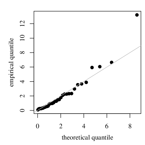
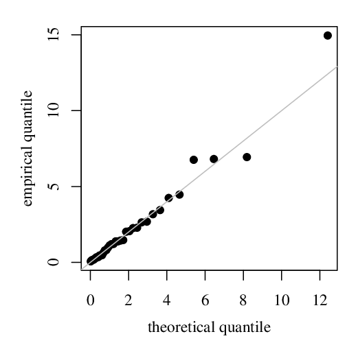
Figure 2 shows the QQ plots of the Mahalanobis distance for the bivariate unit-log-symmetric models considered in Table 4. The QQ plot is a plot of the empirical quantiles of the Mahalanobis distance against the theoretical quantiles of the respective reference distribution (see Section 3.4). Therefore, points falling along a straight line would indicate a good fit. From Figure 2, we see clearly that, with the exception of log-Student- $t$ case, the Mahalanobis distances in the considered models conform relatively well with their reference distributions. We also see that, in all the cases, there is a point away from the reference line, which may be an outlier.

6.2 2022 FIFA World Cup

We now use the data on the 2022 FIFA World Cup to illustrate the model developed in the preceding sections. The data are available at https://www.kaggle.com/. The first variable ( $W_{1}$ ) is the medium pass completion proportion, that is, successful passes between 14 and 18 meters. The second variable ( $W_{2}$ ) is the long pass completion proportion, namely, passes longer than 37 meters; see Table 7.

Table 5 provides descriptive statistics for the variables $W_{1}$ and $W_{2}$ . We observe in the variable $W_{1}$ , the mean and median to be, respectively, $0.454$ and $0.456$ , i.e., the mean is almost equal to the median, which indicates symmetry in the data. The CV is $49.274\%$ , which means a moderate level of dispersion around the mean. Furthermore, the CS value also confirms the symmetry nature. The variable $W_{2}$ has mean equal to $0.365$ and median equal to $0.311$ , which indicates a small positively skewed feature in the distribution of the data. Moreover, the CV value is $69.475\%$ , showing a moderate level of dispersion around the mean. The CS confirms the small skewed nature and the CK value indicates the small kurtosis feature in the data.

Table 5: Summary statistics for the 2022 FIFA World Cup data set.

Variables	$n$	Minimum	Median	Mean	Maximum	SD	CV	CS	CK
$W_{1}$	32	0.769	0.860	0.860	0.931	0.038	4.376	-0.373	-0.194
$W_{2}$	32	0.427	0.556	0.550	0.751	0.075	13.713	0.308	-0.425

Table 6 presents the estimation results for the bivariate unit-log-symmetric models, and these reveal that the log-normal model provides better fit than all other models based on the values of log-likelihood, AIC and BIC.

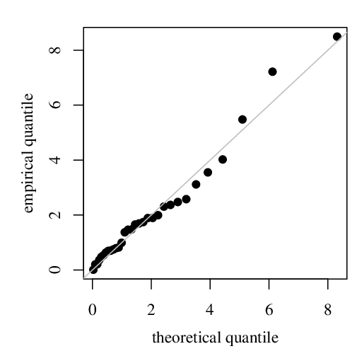
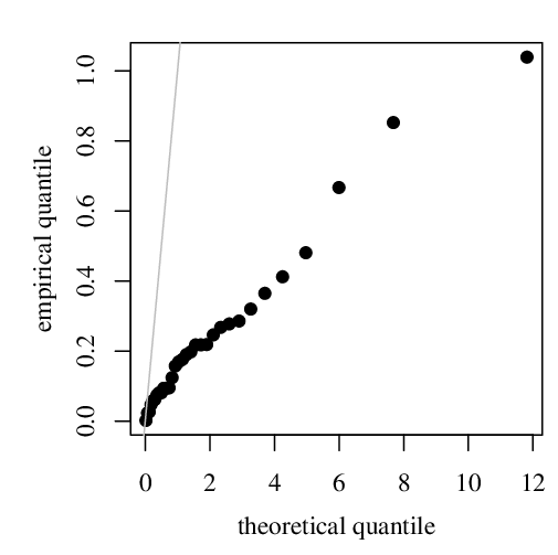
Figure 3 shows the QQ plots of the Mahalanobis distances (see Section 3.4) for the bivariate unit-log-symmetric models considered in Table 6. We see clearly that the log-normal model provides better fit than all other bivariate unit-log-symmetric models.

Table 6: ML estimates (with standard errors in parentheses), and log-likelihood, AIC and BIC values for the indicated bivariate unit-log-symmetric models.


Distribuiton	$\widehat{\eta}_{1}$	$\widehat{\eta}_{2}$	$\widehat{\sigma}_{1}$	$\widehat{\sigma}_{2}$	$\widehat{\rho}$	$\widehat{\nu}$	Log-likelihood	AIC	BIC
Log-normal	1.9872*	0.7953*	0.1364*	0.2089*	0.7343*	–	20.791	-31.581	-24.252
	(0.0479)	(0.0294)	(0.0171)	(0.0261)	(0.0815)
Log-Student- $t$	1.9954*	0.7936*	-0.1257*	-0.1949*	0.7423*	9	20.130	-30.260	-22.931
	(0.0485)	(0.0299)	(0.0178)	(0.0271)	(0.0868)
Log-hyperbolic	1.9908*	0.7942*	0.3956*	0.6088*	0.7378*	10	20.618	-31.236	-23.907
	(0.0482)	(0.0296)	(0.0523)	(0.0800)	(0.0841)
Log-Laplace	1.9908*	0.8089*	0.1563*	0.2425*	0.7471*	–	16.915	-23.830	-16.501
	(0.0023)	(0.0021)	(0.0278)	(0.0415)	(0.0938)
Log-slash	1.9897*	0.7935*	0.1173*	0.1802*	0.7392*	8	20.613	-28.919	-23.898
	(0.0482)	(0.0295)	(0.0154)	(0.0237)	(0.0844)

^∗ significant at 5% level.

7 Conclusions

In this paper, we have proposed a family of bivariate distributions over the unit square. By suitably defining the density generator, we can transform any distribution over the real line into a bivariate distribution over the region $(0,1)\times(0,1)$ . Such a model has several potential applications, since the simultaneous modeling of quantities like proportions, rates or indices frequently arises in applied sciences like economics, medicine, engineering and social sciences. We have discussed several theoretical properties like stochastic representation, quantiles, conditional distributions, independence and moments. We have also carried out a Monte Carlo simulation study and finally demonstrated some applications to soccer data. The present research can be extended in several possible directions. By changing the density generator, numerous special forms of the BULS distribution can be constructed. Furthermore, generalizations to higher dimensions can be studied. We are currently working in these directions and hope to report the findings in a future paper.

Acknowledgements

Roberto Vila and Helton Saulo gratefully acknowledge financial support from CNPq, CAPES and FAP-DF, Brazil.

Disclosure statement

There are no conflicts of interest to disclose.

References

Abdous et al., (2005) Abdous, B., Fougères, A.-L., and Ghoudi, K., Extreme behaviour for bivariate elliptical distributions, Canadian Journal of Statistics, 33:317–334, 2005.
Arnold and Ng, (2011) Arnold, B. C. and Ng, H. K. T., Flexible bivariate beta distributions, Journal of Multivariate Analysis, 102:1194–1202, 2011.
Balakrishnan and Lai, (2009) Balakrishnan, N. and Lai, C-D., Continuous Bivariate Distributions, Springer-Verlag, New York, 2009.
Cox and Hinkley, (1974) Cox, D. R. and Hinkley, D. V., Theoretical Statistics, Chapman and Hall, London, England, 1974.
Davison, (2008) Davison, A. C., Statistical Models, Cambridge University Press, Cambridge, England, 2008.
Deng and Yao, (2018) Deng, X. and Yao, J. (2018). On the property of multivariate generalized hyperbolic distribution and the Stein-type inequality. Communications in Statistics-Theory and Methods, 47:5346–5356.
Fang et al., (1990) Fang, K. T., Kotz, S. and Ng, K. W., Symmetric Multivariate and Related Distributions, Chapman and Hall, London, England, 1990.
Gradshteyn and Ryzhik, (2000) Gradshteyn, I. S. and Ryzhik, I. M., Table of Integrals, Series and Products, Academic Press, San Diego, 2000.
Heckman, (1979) Heckman, J. J., Sample selection bias as a specification error, Econometrica, 47:153–161, 1979.
James, (2004) James, B. R., Probabilidade: um curso em nível intermediário, Projeto Euclides, Brazil, 2004.
Kotz et al., (2001) Kotz, S., Kozubowski, T. J. and Podgórski, K., The Laplace Distribution and Generalizations, John Wiley & Sons, New York, 2001.
Martínez-Flórez et al., (2022) Martínez-Flórez, G., Lemonte, A. J., Moreno-Arenas, G. and Tovar-Falón, R., The bivariate unit-sinh-normal distribution and its related regression model, Mathematics, 10:3125, 2022.
Meintanis, (2007) Meintanis, S. G., Test of fit for Marshall-Olkin distributions with applications, Journal of Statistical Planning and Inference, 137:3954-3963, 2007.
Nadarajah et al., (2017) Nadarajah, S., Shih, S. H., and Nagar, D. K., A new bivariate beta distribution, Statistics, 51:455-474, 2017.
Rohatgi and Saleh, (2015) Rohatgi V. K. and Saleh, A. K. Md. E., An Introduction to Probability Theory and Mathematical Statistics, 3rd edition, John Wiley & Sons, Hoboken, New Jersey, 2015.
Saulo et al., (2017) Saulo, H., Balakrishnan, N., Zhu, X., Gonzales, J. F. B. and Leão, J., Estimation in generalized bivariate Birnbaum-Saunders models, Metrika, 80:427-453, 2017.
Saulo et al., (2022) Saulo, H., Dasilva, A., Leiva, V., Sánchez, L., and Fuente-Mella, H. L. Log-symmetric quantile regression models, Statistica Neerlandica, 76:124–163, 2022.
Saulo et al., (2023) Saulo, H., Vila, R., Cordeiro, S. S. and Leiva, V. Bivariate symmetric Heckman models and their characterization, Journal of Multivariate Analysis, 193:105097, 2023.
Vanegas and Paula, (2016) Vanegas, L. H. and Paula, G. A., Log-symmetric distributions: Statistical properties and parameter estimation, Brazilian Journal of Probability and Statistics, 30:196–220, 2016.
Vila et al., (2022) Vila, R., Balakrishnan, N., Saulo, H. and Protazio, A. Bivariate log-symmetric models: Theoretical properties and parameter estimation, Preprint, Avaliable at https://arxiv.org/pdf/2211.13839.pdf, 2022.
Wang and Genton, (2006) Wang, J. and Genton, M. The multivariate skew-slash distribution. Journal of Statistical Planning and Inference, 136:209–220, 2006.

Appendix A Some additional results

For the convenience of readers, we present here some complementary results relating to Section 3.3.

Definition A.1.

We say that a random variable $X$ follows a univariate generalized hyperbolic (GH) distribution, denoted by $X\sim{\rm GH}(\lambda,\alpha,\delta)$ , if its PDF is given by

\displaystyle f_{\rm GH}(x;\lambda,\alpha,\delta)=\dfrac{(\sqrt{\alpha^{2}}/\delta)^{\lambda}}{\sqrt{2\pi}K_{\lambda}(\delta\sqrt{\alpha^{2}}\,)}\,\,\dfrac{K_{\lambda-1/2}(\alpha\sqrt{\delta^{2}+x^{2}})}{(\sqrt{\delta^{2}+x^{2}}/\alpha)^{1/2-\lambda}},\quad-\infty<x<\infty.

Here, $K_{r}$ is the modified Bessel function of the third kind with index $r$ , $\lambda\in\mathbb{R},\alpha\in\mathbb{R}$ and $\delta>0$ is a scale parameter.

The following result has appeared in a multivariated version in Deng and Yao, 2018.

Proposition A.1 (Hyperbolic generator).

Let $\bm{Z}=(Z_{1},Z_{2})^{\top}$ be a random vector as in Proposition 3.1. If $g_{c}(x)=\exp(-\nu\sqrt{1+x}\,)$ , then the conditional distribution of $Z_{2}$ , given $Z_{1}=x$ , is ${\rm GH}(1,\nu,\sqrt{1+x^{2}}\,)$ and both of its unconditional distributions are ${\rm GH}(3/2,\nu,1)$ .

Proof.

By using (3.4), the joint PDF of $Z_{1}$ and $Z_{2}$ is (see Table 1)

\displaystyle f_{Z_{1},Z_{2}}(x,y)={\nu^{2}\exp(\nu)\over 2\pi(\nu+1)}\,\exp\left(-\nu\sqrt{1+x^{2}+y^{2}}\,\right).

(A.1)

So, the marginal PDF of $Z_{1}$ is given by

	$\displaystyle f_{Z_{1}}(x)=\int_{-\infty}^{\infty}f_{Z_{1},Z_{2}}(x,y)\,{\rm d}y$	$\displaystyle={\nu^{2}\exp(\nu)\over 2\pi(\nu+1)}\,\int_{-\infty}^{\infty}\exp\left(-\nu\sqrt{1+x^{2}+y^{2}}\,\right)\,{\rm d}y$
		$\displaystyle={2\nu^{2}\exp(\nu)\over 2\pi(\nu+1)}\,\int_{0}^{\infty}\exp\left(-\nu\sqrt{1+x^{2}+y^{2}}\,\right)\,{\rm d}y.$

By using Formula 6 of Section 3.46-3.48 of Gradshteyn and Ryzhik, 2000 that $\int_{0}^{\infty}\exp(-a\sqrt{b^{2}+x^{2}}){\rm d}x=bK_{1}(ab)$ , the above integral is

\displaystyle={2\nu^{2}\exp(\nu)\over 2\pi(\nu+1)}\,\sqrt{1+x^{2}}K_{1}(\nu\sqrt{1+x^{2}}\,).

(A.2)

Now, as $K_{3/2}(\nu)=2\sqrt{\pi}\exp(-\nu)(\nu+1)(\nu/2)^{3/2}/\nu^{3}$ , the above espression becomes

\displaystyle={\nu^{3/2}\over\sqrt{2\pi}K_{3/2}(\nu)}\,{K_{1}(\nu\sqrt{1+x^{2}})\over(\sqrt{1+x^{2}}/\nu\,)^{-1}}=f_{\rm GH}(x;3/2,\nu,1)

which proves that $Z_{1}\sim{\rm GH}(3/2,\nu,1)$ . Similarly, we can show that $Z_{2}\sim{\rm GH}(3/2,\nu,1)$ , as well.

On the other hand, from (A.1) and (A.2), and by using the well-known identity $K_{1/2}(z)=\sqrt{\pi/(2z)}\exp(-z)$ , the conditional PDF of $Z_{2}$ , given $Z_{1}=x$ , is obtained as

	$\displaystyle f_{Z_{2}\,\|\,Z_{1}}(y\,\|\,x)=\dfrac{\exp(-\nu\sqrt{1+x^{2}+y^{2}}\,)}{2\sqrt{1+x^{2}}K_{1}(\nu\sqrt{1+x^{2}}\,)}$	$\displaystyle=\dfrac{\nu/\sqrt{1+x^{2}}}{\sqrt{2\pi}K_{1}(\nu\sqrt{1+x^{2}}\,)}\,\dfrac{K_{1/2}(\nu\sqrt{1+x^{2}+y^{2}}\,)}{(\sqrt{1+x^{2}+y^{2}}/\nu)^{-1/2}}$
		$\displaystyle=f_{\rm GH}(x;1,\nu,\sqrt{1+x^{2}}),$

which complete the proof. ∎

The following result has also appeared in a multivariated version in Kotz et al., 2001.

Proposition A.2 (Laplace generator).

Let $\bm{Z}=(Z_{1},Z_{2})^{\top}$ be a random vector as in Proposition 3.1. If $g_{c}(x)=K_{0}(\sqrt{2x}\,)$ , then the conditional distribution of $Z_{2}$ , given $Z_{1}=x$ , is ${\rm GH}(1/2,\sqrt{2},|x|)$ and both of its unconditional distributions are ${\rm Laplace}(0,1/\sqrt{2})$ .

Proof.

By (3.4) and using the definitions of $K_{0}$ and $Z_{g_{c}}$ in Table 1, we have

\displaystyle f_{Z_{1},Z_{2}}(x,y)={1\over\pi}\,K_{0}\left(\sqrt{2(x^{2}+y^{2})}\,\right)={1\over 2\pi}\,\int_{0}^{\infty}{1\over t}\exp\left(-t-{x^{2}+y^{2}\over 2t}\right){\rm d}t.

(A.3)

We then find the marginal density of $Z_{1}$ to be

\displaystyle f_{Z_{1}}(x)=\int_{-\infty}^{\infty}f_{Z_{1},Z_{2}}(x,y)\,{\rm d}y={1\over\sqrt{2}}\,\exp(-\sqrt{2}\,|x|)=f_{\rm L}(x),

(A.4)

where $f_{\rm L}(x)=\exp(-\sqrt{2}\,|x|)/\sqrt{2}$ is the Laplace PDF with scale parameter $1/\sqrt{2}$ ; that is, $Z_{1}\sim{\rm Laplace}(0,1/\sqrt{2})$ . Similarly, we can show that $Z_{2}\sim{\rm Laplace}(0,1/\sqrt{2})$ , as well.

On the other hand, by using (A.3), (A.4) and the well-known identity $K_{1/2}(z)=\sqrt{\pi/(2z)}\exp(-z)$ , the conditional PDF of $Z_{2}$ , given $Z_{1}=x$ , is obtained as

	$\displaystyle f_{Z_{2}\,\|\,Z_{1}}(y\,\|\,x)=\dfrac{\displaystyle{1\over\pi}\,K_{0}\left(\sqrt{2(x^{2}+y^{2})}\,\right)}{\displaystyle{1\over\sqrt{2}}\exp(-\sqrt{2}\,\|x\|)}$	$\displaystyle=\dfrac{(\sqrt{2}/\|x\|)^{1/2}}{\sqrt{2\pi}K_{1/2}(\sqrt{2}\|x\|)}\,K_{0}\left(\sqrt{2}\sqrt{x^{2}+y^{2}}\,\right)$
		$\displaystyle=f_{\rm GH}(x;1/2,\sqrt{2},\|x\|).$

Then, from Definition A.1, we simply have $Z_{2}\,|\,(Z_{1}=x)\sim{\rm GH}(1/2,\sqrt{2},|x|)$ . ∎

Definition A.2.

We say that a random variable $X$ follows an univariate extended slash (ESL) distribution, denoted by $X\sim{\rm ESL}(a,q)$ , if its PDF is given by

\displaystyle f_{\rm ESL}(x;a,q)=\dfrac{\displaystyle\int_{0}^{1}t^{q}\phi(ta)\phi(tx)\,{\rm d}t}{\displaystyle\int_{0}^{1}u^{q-1}\phi(ua)\,{\rm d}u},\quad-\infty<x<\infty,

where $\phi$ denotes the PDF of the standard normal distribution.

If we now choose $a=0$ , the classical slash (SL) PDF is obtained, given by

	$\displaystyle f_{\rm SL}(x;q)$	$\displaystyle=q\int_{0}^{1}t^{q}\phi(tx)\,{\rm d}t,\quad-\infty<x<\infty$
		$\displaystyle={q\,2^{{q\over 2}-1}\over\sqrt{\pi}}\,\|x\|^{-(q+1)}\,\gamma\left({q+1\over 2},{x^{2}\over 2}\right).$

In this case, we denote it by $X\sim{\rm SL}(q)$ .

Proposition A.3 (Slash generator).

Let $\bm{Z}=(Z_{1},Z_{2})^{\top}$ be a random vector as in Proposition 3.1. If $g_{c}(x)=x^{-{(q+2)/2}}\gamma({(q+2)/2},{x/2})$ , then the conditional distribution of $Z_{2}$ , given $Z_{1}=x$ , is ${\rm ESL}(x,q+1)$ and both of its unconditional distributions are ${\rm SL}(q)$ .

Proof.

By (3.4) and using the definition of $Z_{g_{c}}$ in Table 1, the joint PDF of $Z_{1}$ and $Z_{2}$ is given by

	$\displaystyle f_{Z_{1},Z_{2}}(x,y)$	$\displaystyle={q\,2^{{q\over 2}-1}\over\pi}\,(x^{2}+y^{2})^{-{q+2\over 2}}\,\gamma\left({q+2\over 2},{x^{2}+y^{2}\over 2}\right)$
		$\displaystyle=q\int_{0}^{1}t^{q+1}\phi(tx)\phi(ty)\,{\rm d}t.$		(A.5)

So, the marginal PDF of $Z_{1}$ is

	$\displaystyle f_{Z_{1}}(x)=\int_{-\infty}^{\infty}f_{Z_{1},Z_{2}}(x,y)\,{\rm d}y$	$\displaystyle=q\int_{0}^{1}t^{q+1}\phi(tx)\left[\int_{-\infty}^{\infty}\phi(ty)\,{\rm d}y\right]{\rm d}t$
		$\displaystyle=q\int_{0}^{1}t^{q}\phi(tx)\,{\rm d}t=f_{\rm SL}(x;q),$		(A.6)

which proves that (see Definition A.2), $Z_{1}\sim{\rm SL}(q)$ . Similarly, we can show that $Z_{2}\sim{\rm SL}(q)$ .

On the other hand, by (A) and (A), the conditional PDF of $Z_{2}$ , given $Z_{1}=x$ , is obtained as

\displaystyle f_{Z_{2}\,|\,Z_{1}}(y\,|\,x)=\dfrac{\displaystyle\int_{0}^{1}t^{q+1}\phi(tx)\phi(ty)\,{\rm d}t}{\displaystyle\int_{0}^{1}u^{q}\phi(ux)\,{\rm d}u}=f_{\rm ESL}(y;x,q+1).

From Definition A.2, we then find that $Z_{2}\,|\,(Z_{1}=x)\sim{\rm ESL}(x,q+1)$ . ∎

Appendix B Data sets

Table 7: UEFA Champions League and 2022 FIFA World Cup data sets.

	UEFA		FIFA
	W1	W2	W1	W2
1	0.289	0.222	0.888	0.541
2	0.700	0.200	0.815	0.474
3	0.211	0.211	0.907	0.624
4	0.733	0.944	0.891	0.606
5	0.444	0.444	0.827	0.517
6	0.544	0.544	0.898	0.557
7	0.089	0.089	0.856	0.462
8	0.767	0.789	0.861	0.618
9	0.433	0.433	0.890	0.603
10	0.911	0.533	0.860	0.477
11	0.800	0.800	0.920	0.646
12	0.733	0.689	0.894	0.587
13	0.278	0.100	0.913	0.648
14	0.456	0.033	0.849	0.471
15	0.178	0.833	0.781	0.427
16	0.200	0.200	0.828	0.442
17	0.244	0.156	0.864	0.581
18	0.467	0.467	0.820	0.527
19	0.022	0.022	0.846	0.526
20	0.400	0.578	0.879	0.601
21	0.378	0.378	0.860	0.481
22	0.589	0.433	0.885	0.616
23	0.600	0.078	0.862	0.592
24	0.567	0.311	0.769	0.463
25	0.844	0.711	0.845	0.495
26	0.711	0.167	0.846	0.489
27	0.289	0.533	0.931	0.751
28	0.178	0.178	0.863	0.555
29	0.489	0.144	0.856	0.447
30	0.278	0.156	0.879	0.569
31	0.611	0.122	0.812	0.613
32	0.544	0.544	0.841	0.594
33	0.267	0.267	–	–
34	0.489	0.333	–	–
35	0.467	0.033	–	–
36	0.300	0.522	–	–
37	0.311	0.311	–	–

Bivariate distributions on the unit square: Theoretical properties and applications

Abstract

1 Introduction

2 Bivariate unit-log-symmetric model

2.1 BLS distribution

2.2 BULS distribution

3 Some basic properties of the model

3.1 Stochastic representation

Proposition 3.1.

Proof.

Lemma 3.2.

Proof.

3.2 Marginal Quantiles

3.3 Conditional distributions

Lemma 3.3.

Proof.

Theorem 3.4.

Proof.

Corollary 3.5 (Gaussian generator).

Proof.

Corollary 3.6 (Student-tt generator).

Proof.

Corollary 3.7 (Hyperbolic generator).

Proof.

Corollary 3.8 (Laplace generator).

Proof.

Corollary 3.9 (Slash generator).

Proof.

3.4 Squared Mahalanobis Distance

3.5 Independence

Proposition 3.10.

Proof.

Remark 3.11.

3.6 Moments

4 Maximum likelihood estimation

Proposition 4.1.

Proof.

5 Simulation study

6 Application to soccer data

6.1 UEFA Champions League

6.2 2022 FIFA World Cup

7 Conclusions

Acknowledgements

Disclosure statement

References

Appendix A Some additional results

Definition A.1.

Proposition A.1 (Hyperbolic generator).

Proof.

Proposition A.2 (Laplace generator).

Proof.

Definition A.2.

Proposition A.3 (Slash generator).

Proof.

Appendix B Data sets

Corollary 3.6 (Student- $t$ generator).