Coulomb blockade of chiral Majorana and complex fermions far from equilibrium
Abstract
We study charge transport in a single-electron transistor implemented as an interferometer such that the Coulomb blockaded middle island contains a circular chiral Majorana or Dirac edge mode. We concentrate on the regime of small conductance and provide an asymptotic solution in the limit of high transport voltage exceeding the charging energy. The solution is achieved using an instanton-like technique. The distinctions between Majorana and Dirac cases appears when the tunnel junctions are unequal. The main difference is in the offset current at high voltages which can be higher up to 50% in Majorana case. It is caused by an additional particle-hole symmetry of the distribution function in the Majorana case. There is also an eye-catching distinction between the oscillations patterns of the current as a function of the gate charge. We conjecture this distinction survives at lower transport voltages as well.
I Introduction
The effect of Coulomb blockade in a single-electron transistor (SET) Kulik and Shekhter 1975; Averin and Likharev 1986; Ingold and Nazarov 1992; Kamenev and Gefen 1996; Kouwenhoven et al. 1997; Aleiner et al. 2002; Nazarov 1999, a device where Fermi-liquid leads are mediated by a quantum dot, plays an essential role in condensed matter physics, mesoscopics and open quantum systems. The Coulomb spectroscopy and transport through a quantum dot are sensitive to the precise nature of the non-equilibrium steady state, the mechanisms of relaxation, electronic interactions and topological order Altland et al. 2006; Sedlmayr et al. 2006; Altland and Egger 2009; Rodionov et al. 2010; Zazunov et al. 2011; Shnirman et al. 2015; Albrecht et al. 2016; Titov and Gutman 2016; Ludwig et al. 2017; Pikulin et al. 2019; Burmistrov et al. 2020; Ludwig et al. 2020; Dotdaev et al. 2021. The “orthodox” theory of Coulomb blockade is based on rate equations formulated in the basis of different charged states in the island Kulik and Shekhter 1975; Averin and Likharev 1986; Ingold and Nazarov 1992; Kouwenhoven et al. 1997. Such states are well defined for almost isolated quantum dots which have weak tunnel coupling to the leads, i.e, with a small dimensionless conductance, . In this theory, the distribution function in the island is not affected by the the coupling to contacts, i.e., the internal relaxation in the island is assumed to prevail on the characteristic tunneling timescale. In multi-channel limit with , when the Coulomb blockade is weak and the charge is ill defined, the description via the dissipative Ambegaokar-Eckern-Schön (AES) action Ambegaokar et al. 1982; Eckern et al. 1984 for the phase becomes more convenient Altland et al. 2006. In equilibrium, the saddle points of the Matsubara AES action are known as Korshunov instantons Korshunov 1987. These instantons allow one to take into account charge discreteness and obtain the residual, exponentially small gate charge oscillations of the conductance. If the relaxation is weak then the distribution function in the island is a non-Fermi one at finite voltages. It causes a non-equilibrium steady state that can not be captured by the “orthodox” theory or the imaginary time technique, and consequently the real time Keldysh formalism Keldysh 1965; Kamenev 2011 is required. Important recent achievements include the theoretical analysis of strongly non-equilibrium transport using the AES action Altland and Egger 2009, and the generalization of Korshunov instantons to the real-time Keldysh formalism Titov and Gutman 2016 at . In particular, the results of Ref. Altland and Egger 2009 lead directly to the conclusion that the Coulomb blockade is lifted at transport voltages lower than in the “orthodox” theory due to the non-equilibrium distribution function in the island.
In this work, we study the strongly non-equilibrium regime of high voltages that exceed significantly the charging energy of an island, and we assume the strong Coulomb blockade, i.e., the dimensionless conductance is small, . At low voltages one thus expects a strong suppression of the charge transport. At higher voltages the almost Ohmic behavior is accompanied by the offset (deficit) current and residual gate charge oscillations. Here, we were able to describe this high voltage regime asymptotically exact. Instead of using the kinetic equations, which is challenging due to a large number of relevant charge states, we employ a path integral technique and succeed solving the problem by finding a dominant path, an alternative kind of instanton, for the phase variable.
We apply our solution for calculations of the non-equilibrium tunneling density of states (TDoS) and current-voltage relations using the formalism developed by Meir and Wingreen Meir and Wingreen 1992. The devices under consideration are chiral interferometers implemented in hybrid structures with superconductors, topological insulators or quantum anomalous Hall insulators (QAHI) Fu and Kane 2008; He et al. 2017; Shen et al. 2020 (see Fig. 1). They have two Fermi-liquid leads biased by the voltages , and tunnel coupled to the central island. The island hosts a single conducting channel which is either a real Majorana fermion edge mode (the case when the island is in a proximity induced topological superconducting phase) or a complex Dirac one (the case of a normal island in a quantum-Hall topological insulator state). There is an electrostatic gate that induces an offset charge in the island, . The charging energy of the island is with is electron charge and is the total capacitance of the island. The chiral fermions propagate with a velocity along the edge channels. In this case, the Thouless energy, ( is Plank constant), is nothing but level spacing in the ring of the perimeter . (Hereafter we set .) We assume metallic spectrum of the edge modes which means that is sufficiently small. The voltages are limited from above by the energy scale —the absolute value of the superconducting order parameter induced in the topological part of the island—above which other conducting channels or 2D scattering states become relevant. Ultimately, we work under the following assumption,
| (1) |
Moreover, we assume no relaxation to phonons, no electron-electron scattering and zero temperature. The only relaxation mechanism is due to the tunneling to the leads. In this regime the single-particle distribution function is expected to develop a multi-step structure which will play a substantial role below.
II Model
II.1 Keldysh action for the Majorana device
The microscopic description of the charge transport is provided by the Keldysh generating functional
| (2) |
The first path integral is taken over complex fermions, , collected in Nambu spinors and where () are Grassmann fields in left (right) leads; these are chiral states of momenta . The second variable is Majorana edge mode in the island being real Grassmann field defined on a ring with a coordinate . The third one, , is the phase of the superconducting order parameter in the island. depends on a pair of counting fields and (source variables) collected in . They generate the charges that flow from the left () or right () lead into the island during the measurement interval :
| (3) |
The total action is
| (4) |
In the Keldysh technique, the physical time gets doubled, , with the index denoting the upward and backward parts of Keldysh contour . Then, the Keldysh rotation to classical and quantum components of the boson field, and , is performed: .
A coherent dynamics of is governed by the action where the Lagrangian is
| (5) |
Complex fermion dynamics is described by Keldysh actions, , where is a Hamiltonian of chiral fermions and the lead index is . The action in -basis reads where the inverted fermion Green function is
| (6) |
are the Pauli matrices, is an infinitesimal broadening constant. We keep the -basis for fermions while perform the Keldysh rotation to the classical and classical components for the phase, . The functions are determined by zero temperature Fermi distribution functions in the leads, . We assume here that the symmetric voltage bias is applied. The energies of Dirac electrons in the leads are counted from a chemical potential at zero bias.
We apply a uniform gauge transformation (see Appendix A) for the complex fermions in the island, . After the transformation, the floating phase and the yet unknown chemical potential of the -wave superconducting island, , are eliminated from the island’s action; they appear instead in the tunneling action below. One arrives at the stationary Bogolyubov-de Gennes Hamiltonian, which at low energies (below , see Eq. (1)) reduces to the following effective action for chiral edge Majorana modes:
| (7) |
Here, the Lagrangian is diagonal in the Keldysh space, i.e., there is no internal broadening/dissipation. In this case, this kernel is not invertible which means fully unitary dynamics. An introduction of an infinitesimal broadening with some distribution functions is not necessary as it will anyway be overridden by the coupling to the leads. The latter is described by the tunnel action for the low-energy modes, where the above mentioned gauge transformation and the rotation to the Majorana basis is performed,
| (8) |
Here, Majorana field couples to the local fermions in the leads at two points, . The tunnel amplitudes are chosen real. The matrix
| (9) |
captures the gauge transformation mentioned above and the counting field. The yet unknown chemical potential of the island will be found after solving an appropriate kinetic equation. This transformation also means that all energies in the island are counted from . The charge counting variable is an amplitude of the auxiliary quantum field, . It generates the transmitted charge which is a classical observable. Further, for and otherwise. It switches the charge counting on and off at and , respectively.
II.2 Non-equilibrium effective theory for the phase
After the integration over the complex fermions, , and then over the Majorana ones, , the generating functional (2) becomes
| (10) |
Here, is the self-energy for Majorana fermions. It reads
| (11) |
where is the boson-dressed Green function of the lead. The self-energy is singular at the points where the tunnel contacts are located. The presence of two contributions to the self-energy ( and ) reflects the Majorana nature of the island excitations. In the time domain the local Green functions of the leads read where
| (12) |
To analyze the phase dynamics, we develop here an expansion scheme for the logarithm in (10). A naive expansion in the small tunneling amplitude would force us to introduce an infinitesimal broadening in the island with an arbitrary distribution function. However, in such an approach a physical distribution function, dictated by the leads, would emerge only after the infinite summation of higher order contributions. Instead, we extract from a part with a constant in time classical phase , . We transfer the extracted part, , into the zeroth order propagator Ludwig et al. 2017,
| (13) |
which we can invert exactly, and perform an expansion in . Due to the gauge invariance of the problem, does not appear in the final results.
We expand the logarithm in (10) up to the first order in . After that, itself is expanded up to the linear order in since we are interested in the current only. Omitting a constant term, we obtain the following result for the logarithm in (10):
| (14) |
The first term in (14) is the dissipative AES action Ambegaokar et al. 1982; Eckern et al. 1984,
| (15) |
and the second and third terms contain the charges (cf. Eq. (3)) calculated for a certain path, and . These are given by
| (16) |
We will denote the frequencies related to the island by keeping for the leads. This helps us to remember that the energies on the island are counted from the chemical potential. Since is singular in coordinate representation (cf. Eq. 11), one needs to know the Green function at coincident coordinates, and . Comparing the tunneling self-energy and the ballistic propagator, we conclude that the weak tunneling limit corresponds to the condition . This limit is fully equivalent to the condition of small broadening of levels compared to the distance between them, . In this regime, the Green function reads (see Appendix B):
| (17) |
which involves the four-step function
| (18) |
describing the non-Fermi distribution of Majorana fermions. It has the symmetry, , which is preserved for arbitrary and .
The function is singular at where are the energy levels of the island ( and is the number of vortices). To calculate the chemical potential we neglect the fluctuations of phase and assume the constant trajectory and . Then we employ the the charge conservation constraint, , for (cf. Eq. (16)) and obtain
| (19) |
Unlike in the Dirac case, in which the distribution function is a two-step one governed exclusively by the voltages in the leads, in the current Majorana case there are more steps and the chemical potential is important.
III Formalism and Analytical Results
III.1 Dissipative action
We evaluate the AES action of Eq. (15), and obtain
| (20) |
where and are classical and quantum parts of gauge exponents. In the quasi-classical limit, the off-diagonal terms in (20) determine the dissipative dynamics of the phase. They are given by the retarded (advanced) functions, , with the spectra
| (21) |
(see Appendix C). The diagonal term is the Keldysh one responsible for non-equilibrium fluctuations. Its spectrum reads
| (22) |
Here, dimensionless is the coupling strength of the phase to the dissipative environment. It is the probability for a Majorana excitation to leave the island after encircling it once. In the tunneling limit, we have . Also, the two-step distribution of Dirac fermions has been introduced,
| (23) |
In the metallic limit, i.e., small level spacing, we replace the sum over by the integral, , and we obtain the Ohmic spectrum, . The Keldysh kernel reads
| (24) |
As will be shown below, phase trajectories that contribute to the path integral have typical time scales . One can show that for the kernel can be replaced by its zero frequency value, , provided
| (25) |
Here, the asymmetry parameter is defined as
| (26) |
The parameter is given by where
| (27) |
and
| (28) |
Neglecting the frequency dependence of the kernel at high voltages is similar to the common approximation for a classical noise at high temperatures. In this case, the kernel in (20) becomes local, and the AES action assumes the form, , where the effective dissipative Lagrangian reads
| (29) |
At low voltages, , the AES kernel becomes non-local in time and our approach ceases to be accurate.
III.2 Formula for the current. Tunneling density of states
Due to the non-zero no charge accumulation can occur on the island in the long time limit. Therefore, at we expect . Then we are allowed to consider the following symmetrized form for the current, . Here, the average is taken over all trajectories, . After some algebra with Eq. (16), we arrive at the formula for the current
| (30) |
where the dimensionless conductance is . As shown by Meir and Wingreen Meir and Wingreen 1992, the non-equilibrium state of the island is hidden in the normalized TDoS . In the metallic limit, we obtain
| (31) |
The non-trivial contribution in (31) is provided by
| (32) |
where are the bosonic propagators. For brevity, the phase variables are written in -basis. The propagators obey the following symmetry, .
We note that the phase propagators can be written as the averages, and , with the Heisenberg bosonic operators and . These are the ladder operators of the complex bosonic mode acting in a space of different charge states. Hence, the Fourier transformed function describes the non-equilibrium excitations spectrum in the capacitor.
III.3 SET with the Dirac island
So far, we have considered the Majorana edge mode in the island. Here, we provide the analogous calculations for a device with a normal island that hosts a Dirac edge mode. The action is expressed now in terms of a complex field . There are following distinctions from the Majorana case. First, the non-equilibrium distribution function has the well-known double step structure, , which is not particle-hole symmetric, i.e. , except the limit of fully symmetric setup, . Second, in the formula for the current,
| (33) |
we have . Note that the chemical potential does not influence the result in the Dirac case. Indeed, introducing , i.e., counting the energy from zero, we see that the distribution function does not depend on . The third distinction is that the prefactor in (29) is replaced by
| (34) |
It follows from the Keldysh kernel in the Dirac case, which reads
| (35) |
Similar to the Majorana case, the frequency dependence of this kernel can be neglected and our approach is accurate if .
III.4 Path integration and the instanton. Boson propagator
In this Subsec. III.4 we consider the cases of Majorana and Dirac in parallel, thus, we omit the indices “M” and “D” in . Calculation of boson exponents in (32) is based on the following representation of the path integral,
| (36) |
Here, we have introduced
| (37) |
which does not contain classical components of the phase. We have also introduced
| (38) |
which couples linearly to . The linearity of the action in (36) with respect to plays the central role in our solution. We remind that the exclusively linear dependence on is based on two approximations: the high voltage and the Ohmic spectrum of the island. The linearity in allows one to integrate this field out and obtain a functional delta-distribution, . Therefore, the remaining path integral over is restricted by a manifold of trajectories satisfying with the boundary condition . Analysing we now restrict the allowed trajectories. We note that has an imaginary part . It provides a selection rule for the trajectories: only if , . We find that only a single solution of the first order differential equation satisfies this selection rule, . Therefore, the result of the path integration for the boson propagators reads
| (39) |
Note the combination of theta functions in the r.h.s. of the equation for the quantum trajectory, , plays a role of an external force. It switches on at and off at (assuming ). Consider first the case of zero force when the equation is uniform, , i.e., when . It has a set of trivial solutions,
| (40) |
and the instanton-like ones,
| (41) |
with . Here, the constant determines the instanton center and the time scale is inverse proportional to the charging energy, . The instanton has slow dynamics on the long -like time scale, , due to .
Consider the second case when the force is switched on () and the equation becomes . We neglect the sine term due to small prefactor and obtain a rapidly growing linear solution
| (42) |
up to small oscillations with an amplitude .
We have to match the linear solution (42) in the region with the solutions in the remaining two regions, and . The analysis shows that, in order to satisfy the above selection rules, the solution in the region should be of the instanton form (41) and in the other region, , the constant one, Eq. (40), with an even . The matching conditions (continuity of the solution) uniquely determine free parameters and , as well as the sign of the instanton function, and the even integer , where we added the subscript to emphasize the -dependence. In particular, we have
| (43) |
where the floor function returns the greatest integer less than or equal to . Note that the integer valued function is odd, .
After some algebra, we find the final result for the quantum trajectory at :
| (44) |
The view of the solution is shown in Fig. 2 for different ratios. The instanton tail in (44) reads
| (45) |
where the discrete valued function , which determines the overall sign of (45), is given by .
Finally, one finds for the boson correlator for arbitrary :
| (46) |
This is an oscillating function of multiplied by a decaying envelope determined by .
Neglecting small decay in (46), the following spectrum of excitations is obtained,
| (47) |
It is a ladder of levels, , corresponding to excitations between the states with energies and where is the energy of a state with excess electrons in the island. (We note that the singularities will be slightly smoothened by the frequency when the is taken into account.) The envelope spectral function is
| (48) |
It is an odd function of , . Its negative (positive) values correspond to rates of an absorption (emission) of an electron by a lead at the energy .
In the high voltage regime we estimate that the weights are significant up to . This estimate for determines the number of the charge states that participate in the transport.
III.5 Asymptotic expressions
Let us come back to the expressions for the currents (30) and (33) and analyze some important cases. We focus on the asymptotic behavior at voltages and integrate over and analytically. In this regime the decay in (46) is negligible. The following identities for the Fourier transformations of distribution functions, , are used: and For the difference in occupation numbers in the leads, , we have Then the currents read:
| (49) |
The integrals in (49) can be split into a sum of integrals over intervals , . Their integrands have each a narrow peak in every interval. The peak at is given by a smoothened singularity in . In this case, at the relevant time scale of . The integral for yields the offset current, . Note that it does not depend on and is proportional to . Integrals over the other peaks are responsible for the part of the current, , showing the gate charge oscillations. Their amplitude is much smaller than that of the offset current. This means that at high voltages the strong Coulomb blockade is weakened and the charge on the island is not well defined. For the calculation of the boson correlator becomes important. In a -vicinity of -th peak, where , it reads . Therefore, for both systems the current can be written as
| (50) |
III.6 Offset current
The difference between Majorana and Dirac fermions is most prominent for asymmetric systems. We obtain the following asymptotic results () for the offset current. In Majorana case we get
| (51) |
In comparison, in Dirac case we find
| (52) |
for an arbitrary value of . Therefore, the deficit current in the Majorana case (cf. Eq. (51)) is up to 3/2 times larger that that in the Dirac case.
III.7 Gate charge oscillations
We obtain the following asymptotic result at large voltages for Dirac case:
| (53) |
There is an exponential decay of oscillations’ amplitude as a function of . The gate charge oscillations pattern is given by the function . (The function returns a fractional part of .) It is found after the integration over in Gaussian approximation and further summation over 11 1 The sums or are reduced to the polylogarithm function which has the property for real ..
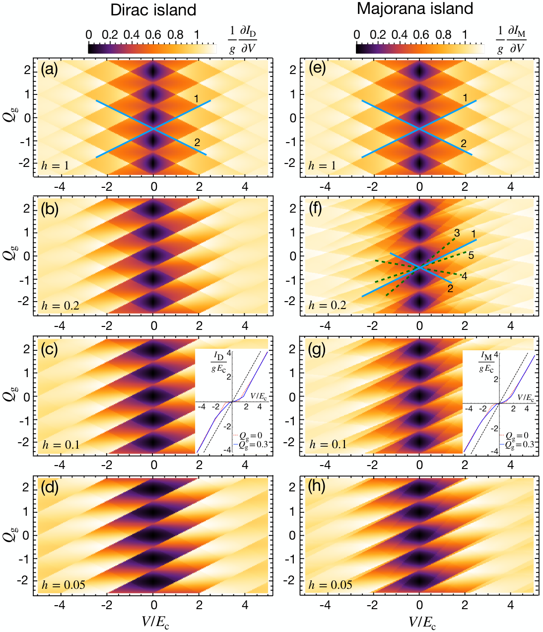
The function has discontinuous derivatives. Namely, and , which satisfy the condition , determine border lines of the so called Coulomb diamond in the differential conductance map. As seen from (53), there are two sets of border lines, (). In asymmetric limit with the lines are suppressed.
In Majorana case the result in general case is more cumbersome:
| (54) |
The terms with and in the sum (54) provide the same border lines, , as in the Dirac case. Other terms define three additional sets of lines: and . Note that depend on and, hence, make the patterns more complicated. We also find that in two particular cases, fully symmetric () and absolutely asymmetric systems ( or ), the patterns for and coincide.
III.8 Graphical presentation of the results
In Fig. 3 we plot the normalized differential conductance as a function of the gate charge and transport voltage for the Dirac [panels (a)-(d)] and Majorana [panels (e)-(h)] devices. Data are found after an exact integration over time in (49). These plots demonstrate the vanishing of the border line at small in strongly asymmetric Dirac devices according to asymptotic result (53). Also, we observe the emerging of three additional border lines [panel (f)], , in Majorana device at predicted by (54).
In Fig. 3 we used our formalism down to zero voltages. Quantitatively, the differential conductance at lower voltages, obtained in our formalism, is not accurate. We are confident, however, that the pattern is qualitatively correct and reflects features of the strong Coulomb blockade behavior.
In asymmetric junctions, the exponentaily small oscillatory contributions are not symmetric under change of the voltage sign , i.e., . The exception is the points () where the poles of are symmetric with respect to . This asymmetry is more visible at low voltages, as shown in the insets in [panels (c), (g)]. It points to a possible diode-like behavior of the asymmetric devices at low .
In Fig. 4 we plot non-equilibrium TDoS, and , which demonstrate a structure of the Coulomb gap. Note that in the Majorana case we always have symmetric TDoS around the chemical potential (dashed line) for any . It is dictated by the particle-hole symmetry of . In Fig. 5 we demonstrate the broadening of the Coulomb gap when the voltage increases. Shaded regions stand for the energy domain, the states from which contribute to the electric current.
IV Discussion
The instanton-like solution presented in Eq. (44) provides only the quantum component of the phase. At the same time, the classical component is not uniquely defined and we have to integrate over all its realizations. This is precisely the difference from the non-equilibrium instanton approach developed in Ref. Titov and Gutman 2016. This approach is valid for , i.e., for the weak Coulomb blockade, and the instanton trajectory fixes both quantum and classical phase components. In contrast, in our case , the Coulomb blockade is strong at low voltages and is lifted at voltages higher than the charging energy.
Our approach based on the AES action allows us to reproduce quantitatively some already known results obtained within charge representation. This is the offset current, which is a characteristic feature of charging effects at high voltages. In the Dirac case we found , which fully coincides with the offset current in the single tunnel junction with dimensionless conductance Averin and Likharev 1986. Another example is the threshold voltage for and , which is two times lower than that in the “orthodox” theory. This result can be easily obtained from Ref. Altland and Egger 2009 and is due to the non-equilibrium distribution function in the dot. The Coulomb blockade is lifted above this threshold. We also reproduce the threshold value (see Fig. 3 [panel (a)]).
One of the central results is the unconventional offset current found for the Majorana island, , where the non-universal prefactor (cf. Eq. (28)) depends on the asymmetry of the SET. This could serve as an evidence of the non-equilibrium chiral Majorana fermions in the island. In addition, the gate charge oscillations show distinctive features in the Majorana case, as shown in Fig. 3 [panel (f)]. Such measurements could provide an alternative to the interferometry Fu and Kane 2009; Akhmerov et al. 2009; Strübi et al. 2015; Strübi et al. 2011; Li et al. 2012; Shapiro et al. 2016; Shapiro et al. 2017; Shapiro et al. 2018; Chung et al. 2011; Liu and Trauzettel 2011; Hou et al. 2013 or time resolved transport Lian et al. 2018; Beenakker et al. 2019; Hassler et al. 2020; Beenakker and Oriekhov 2020; Adagideli et al. 2020; Shapiro et al. 2021 in Majorana devices.
V Summary
In this work, we studied the non-equilibrium transport in single-electron transistors where the strong Coulomb blockade is suppressed by large voltages. Two different kinds of quantum dots were considered. These are the islands with chiral Dirac or chiral Majorana circular modes. These could be the edge states of the usual or anomalous quantum Hall insulators (Dirac) or of the proximity-induced 2D topological superconductors (Majorana). The results of this work are twofold. First, we calculated the non-equilibrium tunneling density of states and current-voltage relations. We found an unusual behavior of the offset current in the Majorana case. There are also distinctive features in the residual gate charge oscillations of the transport current (Coulomb diamond) in the Majorana case. Second, on the methodological level, we developed an instanton-like approach in the Keldysh formalism in the limit of small conductances and high voltages.
Acknowledgements.
This research was financially supported by the DFG Grants No. MI 658/12-1, MI 658/13-1, SH 81/6-1, and by RFBR Grant No. 20-52-12034.References
- Kulik and Shekhter (1975) I. Kulik and R. Shekhter, Zhur. Eksper. Teoret. Fiziki 68, 623 (1975).
- Averin and Likharev (1986) D. V. Averin and K. K. Likharev, Journal of Low Temperature Physics 62, 345 (1986).
- Ingold and Nazarov (1992) G.-L. Ingold and Y. V. Nazarov, in Single charge tunneling (Springer, 1992) pp. 21–107.
- Kamenev and Gefen (1996) A. Kamenev and Y. Gefen, Phys. Rev. B 54, 5428 (1996).
- Kouwenhoven et al. (1997) L. P. Kouwenhoven, G. Schön, and L. L. Sohn, “Introduction to mesoscopic electron transport,” in Mesoscopic Electron Transport, edited by L. L. Sohn, L. P. Kouwenhoven, and G. Schön (Springer Netherlands, Dordrecht, 1997) pp. 1–44.
- Aleiner et al. (2002) I. Aleiner, P. Brouwer, and L. Glazman, Physics Reports 358, 309 (2002).
- Nazarov (1999) Y. V. Nazarov, Phys. Rev. Lett. 82, 1245 (1999).
- Altland et al. (2006) A. Altland, L. Glazman, A. Kamenev, and J. Meyer, Annals of Physics 321, 2566 (2006).
- Sedlmayr et al. (2006) N. Sedlmayr, I. V. Yurkevich, and I. V. Lerner, EPL (Europhysics Letters) 76, 109 (2006).
- Altland and Egger (2009) A. Altland and R. Egger, Phys. Rev. Lett. 102, 026805 (2009).
- Rodionov et al. (2010) Y. I. Rodionov, I. S. Burmistrov, and N. M. Chtchelkatchev, Phys. Rev. B 82, 155317 (2010).
- Zazunov et al. (2011) A. Zazunov, A. L. Yeyati, and R. Egger, Phys. Rev. B 84, 165440 (2011).
- Shnirman et al. (2015) A. Shnirman, Y. Gefen, A. Saha, I. S. Burmistrov, M. N. Kiselev, and A. Altland, Phys. Rev. Lett. 114, 176806 (2015).
- Albrecht et al. (2016) S. M. Albrecht, A. P. Higginbotham, M. Madsen, F. Kuemmeth, T. S. Jespersen, J. Nygård, P. Krogstrup, and C. M. Marcus, Nature 531, 206 (2016).
- Titov and Gutman (2016) M. Titov and D. B. Gutman, Phys. Rev. B 93, 155428 (2016).
- Ludwig et al. (2017) T. Ludwig, I. S. Burmistrov, Y. Gefen, and A. Shnirman, Phys. Rev. B 95, 075425 (2017).
- Pikulin et al. (2019) D. Pikulin, K. Flensberg, L. I. Glazman, M. Houzet, and R. M. Lutchyn, Phys. Rev. Lett. 122, 016801 (2019).
- Burmistrov et al. (2020) I. S. Burmistrov, Y. Gefen, D. S. Shapiro, and A. Shnirman, Phys. Rev. Lett. 124, 196801 (2020).
- Ludwig et al. (2020) T. Ludwig, I. S. Burmistrov, Y. Gefen, and A. Shnirman, Phys. Rev. Res. 2, 023221 (2020).
- Dotdaev et al. (2021) A. Dotdaev, Y. Rodionov, and K. Tikhonov, Physics Letters A 419, 127736 (2021).
- Ambegaokar et al. (1982) V. Ambegaokar, U. Eckern, and G. Schön, Phys. Rev. Lett. 48, 1745 (1982).
- Eckern et al. (1984) U. Eckern, G. Schön, and V. Ambegaokar, Phys. Rev. B 30, 6419 (1984).
- Korshunov (1987) S. Korshunov, JETP Lett 45 (1987).
- Keldysh (1965) L. V. Keldysh, Sov. Phys. JETP 20, 1018 (1965).
- Kamenev (2011) A. Kamenev, Field Theory of Non-Equilibrium Systems (Cambridge University Press, Cambridge, UK, 2011).
- Meir and Wingreen (1992) Y. Meir and N. S. Wingreen, Phys. Rev. Lett. 68, 2512 (1992).
- Fu and Kane (2008) L. Fu and C. L. Kane, Phys. Rev. Lett. 100, 096407 (2008).
- He et al. (2017) Q. L. He, L. Pan, A. L. Stern, E. C. Burks, X. Che, G. Yin, J. Wang, B. Lian, Q. Zhou, E. S. Choi, K. Murata, X. Kou, Z. Chen, T. Nie, Q. Shao, Y. Fan, S.-C. Zhang, K. Liu, J. Xia, and K. L. Wang, Science 357, 294 (2017).
- Shen et al. (2020) J. Shen, J. Lyu, J. Z. Gao, Y.-M. Xie, C.-Z. Chen, C.-w. Cho, O. Atanov, Z. Chen, K. Liu, Y. J. Hu, K. Y. Yip, S. K. Goh, Q. L. He, L. Pan, K. L. Wang, K. T. Law, and R. Lortz, Proceedings of the National Academy of Sciences 117, 238 (2020).
- (30) The sums or are reduced to the polylogarithm function which has the property for real .
- Fu and Kane (2009) L. Fu and C. L. Kane, Phys. Rev. Lett. 102, 216403 (2009).
- Akhmerov et al. (2009) A. R. Akhmerov, J. Nilsson, and C. W. J. Beenakker, Phys. Rev. Lett. 102, 216404 (2009).
- Strübi et al. (2015) G. Strübi, W. Belzig, T. L. Schmidt, and C. Bruder, Physica E: Low-dimensional Systems and Nanostructures 74, 489 (2015).
- Strübi et al. (2011) G. Strübi, W. Belzig, M.-S. Choi, and C. Bruder, Phys. Rev. Lett. 107, 136403 (2011).
- Li et al. (2012) J. Li, G. Fleury, and M. Büttiker, Phys. Rev. B 85, 125440 (2012).
- Shapiro et al. (2016) D. S. Shapiro, A. Shnirman, and A. D. Mirlin, Phys. Rev. B 93, 155411 (2016).
- Shapiro et al. (2017) D. S. Shapiro, D. E. Feldman, A. D. Mirlin, and A. Shnirman, Phys. Rev. B 95, 195425 (2017).
- Shapiro et al. (2018) D. S. Shapiro, A. D. Mirlin, and A. Shnirman, Phys. Rev. B 98, 245405 (2018).
- Chung et al. (2011) S. B. Chung, X.-L. Qi, J. Maciejko, and S.-C. Zhang, Phys. Rev. B 83, 100512(R) (2011).
- Liu and Trauzettel (2011) C.-X. Liu and B. Trauzettel, Phys. Rev. B 83, 220510(R) (2011).
- Hou et al. (2013) C.-Y. Hou, K. Shtengel, and G. Refael, Phys. Rev. B 88, 075304 (2013).
- Lian et al. (2018) B. Lian, X.-Q. Sun, A. Vaezi, X.-L. Qi, and S.-C. Zhang, Proceedings of the National Academy of Sciences 115, 10938 (2018).
- Beenakker et al. (2019) C. W. J. Beenakker, P. Baireuther, Y. Herasymenko, I. Adagideli, L. Wang, and A. R. Akhmerov, Phys. Rev. Lett. 122, 146803 (2019).
- Hassler et al. (2020) F. Hassler, A. Grabsch, M. J. Pacholski, D. O. Oriekhov, O. Ovdat, I. Adagideli, and C. W. J. Beenakker, Phys. Rev. B 102, 045431 (2020).
- Beenakker and Oriekhov (2020) C. Beenakker and D. Oriekhov, SciPost Physics 9, 080 (2020).
- Adagideli et al. (2020) I. Adagideli, F. Hassler, A. Grabsch, M. Pacholski, and C. Beenakker, SciPost Phys. 8, 13 (2020).
- Shapiro et al. (2021) D. S. Shapiro, A. D. Mirlin, and A. Shnirman, Phys. Rev. B 104, 035434 (2021).
- Altland and Simons (2010) A. Altland and B. D. Simons, Condensed matter field theory (Cambridge university press, 2010).
Appendix A Gauge transformation
The Bogolyubov-de Gennes (BdG) Hamiltonian of the 2D topological insulator electrons (, ) in a proximity with -wave superconducting island with the pairing potential reads
| (55) |
The Hamiltonian describes the topological part of the island, is the spin index and is the Pauli matrix in the spin space. The pairing potential, , appears after a Hubbard-Stratonovich decoupling of an interaction term in the superconducting island. The superconducting phase involves the zero mode , which is the yet unknown chemical potential in the superconductor. The non-zero modes are captured by . The potential appears after another Hubbard-Stratonovich transformation that decouples the charging energy in the Hamiltonian. It reads as where is its zero mode and involves all non-zero ones. The gauge transformation, which allows us to eliminate the phase dependence from the order parameter and make it real, , reads as
| (56) |
As a result, the diagonal part of the BdG Hamiltonian changes accordingly,
| (57) |
The Anderson-Higgs mechanism in the superconductor suppresses the non-stationary term in (57) Altland and Simons 2010. Thus, we obtain the Josephson relation between the phase and potential, . The zero modes, and , are determined by global conditions, e.g., the capacitive relation between the charge and the potential, or the conservation of current, the latter being the main subject of our calculation. We arrive at the stationary BdG Hamiltonian (55) with at the diagonal, which we assume to be in the superconducting topological phase with the gap . The low energy excitations of (55) are assumed to be the chiral Majorana edge modes, , described by the effective action (7). Assuming that transport voltages are smaller than and, possibly, the topological gap, the linear dispersion of the Majorana eigenstates is not affected by the presence of in the BdG Hamiltonian. The gauged away phase, , appears in the tunneling action (8).
Appendix B Calculation of the Green function of the chiral fermions in the island
In this Appendix we show that the local Green functions of chiral fermion at the contact points, and , are equal and are denoted by in (17). To derive explicitly, consider the Dyson equation for the coordinate dependent Green function of the circular chiral fermions :
| (58) |
The stationary integral-differential operator , which account for the presence of the contacts, is given by (13). After the Fourier transformation, Eq. (58) yields
| (59) |
We introduced here the self-energies related to the left and right tunnel contacts, , where . Substituting here the lead’s Green functions from (12), the self-energies read
| (60) |
The next step is the Fourier transformation in a basis of eigenstates of an isolated Majorana edge mode of the length :
| (61) |
The eigenstates read () where the wave vectors and energies are given by and , respectively. Here, is an integer number, which is determined by the presence of Berry phase and the number of vortices in the superconductor. Performing the direct and then, the inverse Fourier transformations, we obtain two equations for and :
| (62) |
The function has been introduced. We need to obtain the expressions for and . They follow from (62):
| (63) |
The obtained Green functions are given by a sequence of peaks near . In the limit when the peak width, , is much smaller than the level spacing, , these can be replaced by delta functions. This condition of small peak broadening is equivalent to the tunnel approximation, . To obtain the result in this limit, one has to drop all terms in the sum in except those which correspond to being in the vicinity of , i.e., the following replacement, . Reducing the result of the matrix inversion in (63) to a Lorentzian form and approximating the Lorentzians by the delta functions, we obtain the result (17):
| (64) |
where the non-Fermi distribution function of the Majorana fermions reads
| (65) |
Appendix C Derivation of the AES action
The derivation of the AES action (20) from (15) involves the following transformation under the trace
| (66) |
We substitute here the Majorana Green function from (17) and lead’s Green function from (12), as well as the matrix from (9) (that depends on the field ). The symmetry of the Majorana Green function, , has been exploited here. To obtain expression (15) we subtract the divergent stationary part from (66). As a result, after the Keldysh rotation, we obtain the AES action (20) with and defined by Eqs. (21) and (22). The distributions and , which determine the kernels and , originate from the dot’s and leads’ Green functions, and .