跳到论文正文
W Papers独立论文阅读器 arXiv:2301.04853 论文正文 计算阅读时间 · 0%
引用这篇论文根据当前论文元数据生成,正式投稿前建议核对。


License: arXiv.org perpetual non-exclusive license
arXiv:2301.04853v2 [econ.EM] 16 Jan 2023

Testing for Coefficient Randomness in Local-to-Unity Autoregressions

Mikihito Nishi Note: I am greatly indebted to Eiji Kurozumi, my advisor, for discussions and his help, support and encouragement. I am also grateful to Mototsugu Shintani and Yohei Yamamoto for their helpful comments. All errors are mine. Address correspondence to: Graduate School of Economics, Hitotsubashi University, 2-1 Naka, Kunitachi, Tokyo 186-8601, Japan; e-mail: ed225007@g.hit-u.ac.jp Affiliation: Graduate School of Economics, Hitotsubashi University
August 11, 2026
Abstract

In this study, we propose a test for the coefficient randomness in autoregressive models where the autoregressive coefficient is local to unity, which is empirically relevant given the results of earlier studies. Under this specification, we theoretically analyze the effect of the correlation between the random coefficient and disturbance on tests’ properties, which remains largely unexplored in the literature. Our analysis reveals that the correlation crucially affects the power of tests for coefficient randomness and that tests proposed by earlier studies can perform poorly when the degree of the correlation is moderate to large. The test we propose in this paper is designed to have a power function robust to the correlation. Because the asymptotic null distribution of our test statistic depends on the correlation ψ\psi between the disturbance and its square as earlier tests do, we also propose a modified version of the test statistic such that its asymptotic null distribution is free from the nuisance parameter ψ\psi. The modified test is shown to have better power properties than existing ones in large and finite samples.

Keywords: random coefficient autoregression, local to unity, Bonferroni test

JEL Codes: C12, C22

1 Introduction

In this paper, we consider the random-coefficient autoregressive (RCA) model,

yt=(ρ+ωvt)yt−1+εt,t=1,2,⋯,T,\displaystyle y_{t}=(\rho+\omega v_{t})y_{t-1}+\varepsilon_{t},\ \ t=1,2,\cdots,T, (1)

where (εt,vt)′(\varepsilon_{t},v_{t})^{\prime} is a random vector with 𝔼⁡[εt]=𝔼⁡[vt]=0\mathbb{E}[\varepsilon_{t}]=\mathbb{E}[v_{t}]=0 and 𝕍⁡[vt]=1\mathbb{V}[v_{t}]=1. Model (1) is a generalization of the usual AR(1) model, in that the autoregressive coefficient fluctuates over time around its mean ρ\rho with variance ω2\omega^{2}, instead of being constant at ρ\rho. Since Nicholls and Quinn 1982, much attention has been paid to the estimation and inference theory of model (1); see, for example, Hwang and Basawa 2005, Aue and Horváth 2011, Horváth and Trapani 2019 and references therein.

One aspect of the inferential theory for (1) that has attracted econometricians and statisticians is how to test the hypothesis of ω2=0\omega^{2}=0, that is, how to test the null hypothesis of the usual autoregressive specification against the RCA alternative. Nicholls and Quinn 1982 and Lee 1998 proposed test statistics for testing H0:ω2=0H_{0}:\omega^{2}=0 under the stationarity condition ρ2+ω2<1\rho^{2}+\omega^{2}<1. Nagakura 2009a showed the Lee 1998 test statistic has the same asymptotic null distribution when ρ=1\rho=1 as when |ρ|<1|\rho|<1.11 1 Nagakura 2009b also showed the Lee 1998 test is consistent when ρ2+ω2>1\rho^{2}+\omega^{2}>1 and some other conditions hold. However, he did not show the test statistic has the same limiting null distribution when ρ>1\rho>1 as when |ρ|≤1|\rho|\leq 1. The condition, ρ2+ω2≤1\rho^{2}+\omega^{2}\leq 1, which these tests rest on, however, is restrictive and limits their applicability in practice, in view of the empirical analyses by Hill and Peng 2014 and Horváth and Trapani 2019. They applied model (1) to several macroeconomic variables and estimated ρ\rho to be near 1 for most of the variables, with ρ\rho estimated to be greater than 1 for some. For instance, the ρ\rho estimates obtained by Horváth and Trapani 2019 took values between 0.9884 and 1.0021. Their results indicate that nonstationary RCA models where ρ2+ω2\rho^{2}+\omega^{2} and ρ\rho may be greater than 1 with ρ\rho near unity are empirically relevant, and thus testing procedures are required that are valid under these conditions. Horváth and Trapani 2019 proposed a test statistic for H0:ω2=0H_{0}:\omega^{2}=0 valid under the nonstationarity conditions (as well as under the stationarity conditions).

Another insight earlier studies provide is that the variation of the autoregressive root is smaller (if it exists) than assumed in the extant literature. For example, according to the empirical analysis conducted by Horváth and Trapani 2019, 4 variables out of 7 were estimated to have positive variance (ω2>0\omega^{2}>0) in their coefficient, which is between 7.2×10−57.2\times 10^{-5} and 8.2×10−38.2\times 10^{-3}. However, Horváth and Trapani 2019 studied the finite-sample power of their test only for ω2≥2.5×10⁻¹\omega^{2}\geq 2.5\times 10^{-1}, which are of larger magnitude than observed in practice (as long as macroeconomic variables are concerned). 22 2 Horváth and Trapani 2022 applied the RCA model to a cryptocurrency index and estimated ω2\omega^{2} to be around 10−110^{-1}. Therefore, it is unclear whether their test performs well when ω2\omega^{2} is of small magnitude that seems to be typical in empirical studies. In fact, their test has almost no distinguishing power when ω2\omega^{2} is relatively small, as our simulation studies will reveal.

Given these observations, we consider model (1) with ρ\rho near unity and ω2\omega^{2} near zero and employ the following near unit root RCA model:

yt=(ρT+ωT​vt)​yt−1+εt,\displaystyle y_{t}=(\rho_{T}+\omega_{T}v_{t})y_{t-1}+\varepsilon_{t}, (2)

where ρT=1+a/T\rho_{T}=1+a/T and ωT=c/T3/4\omega_{T}=c/T^{3/4}. When ωT2=0\omega_{T}^{2}=0, (2) is the popular (conventional) local-to-unity AR(1) model. This specification has been useful in analyzing the power of unit root tests (Elliott et al. 1996) and in developing estimation and inference theory for models involving persistent variables (Phillips 1987; Stock 1991; Campbell and Yogo 2006; Phillips 2014, see, inter alia,). The local-to-zero variance ωT2=c2/T3/2\omega_{T}^{2}=c^{2}/T^{3/2} has been employed under ρT=1\rho_{T}=1 by McCabe and Smith 1998 and Nishi and Kurozumi 2022 to derive and compare the local asymptotic power functions of unit root tests of ω2=0\omega^{2}=0 against ω2>0\omega^{2}>0. Introducing the local-to-zero variance provides us with a convenient framework in which we can evaluate power functions of several tests against the alternatives that are close to the null of ω2=0\omega^{2}=0 and seem relevant for empirical applications.33 3 For example, when T=200T=200 and 0<c2≤500<c^{2}\leq 50, the variance ωT2\omega_{T}^{2} takes values between 0 and 1.8×10−21.8\times 10^{-2}. Model (2) integrates these two local-to-unit-root parametrizations, thereby rendering itself an empirically relevant random-coefficient model.

In the literature, testing procedures for H0:ω2=0H_{0}:\omega^{2}=0 have often been studied in the special case with ρT=1\rho_{T}=1. Such a model is called stochastic unit root (STUR) model. Test statistics for H0:ω2=0H_{0}:\omega^{2}=0 in the STUR model have been proposed by earlier studies, including McCabe and Tremayne 1995, Leybourne et al. 1996 and Distaso 2008. Moreover, McCabe and Smith 1998 and Nishi and Kurozumi 2022 analyzed the power properties of several tests for H0:ω2=0H_{0}:\omega^{2}=0 under the STUR modelling. On the one hand, the STUR model is a generalization of the pure unit root model, which is a main reason authors have paid much attention to it. But on the other hand, the assumption of ρT\rho_{T} exactly being unity is a restrictive condition that is unlikely to hold in empirical analysis. Our model, (2), generalizes the STUR model by allowing ρT\rho_{T} to take a value different from unity (but near it), which is a more realistic assumption given the empirical analyses conducted by earlier studies.

Nishi and Kurozumi 2022 revealed that, under the STUR (ρT=1\rho_{T}=1) modelling with Corr⁡(εt,vt)=0\mathrm{Corr}(\varepsilon_{t},v_{t})=0, the test for H0:ω2=0H_{0}:\omega^{2}=0 proposed by Lee 1998 and Nagakura 2009a (hereafter, LN) has a higher local asymptotic power function than other tests. We will demonstrate that this is also the case when ρT=1+a/T\rho_{T}=1+a/T and Corr⁡(εt,vt)=0\mathrm{Corr}(\varepsilon_{t},v_{t})=0. In this paper, however, it will be shown that the LN test can perform poorly when Corr⁡(εt,vt)≠0\mathrm{Corr}(\varepsilon_{t},v_{t})\neq 0, for both the cases ρT=1\rho_{T}=1 and ρT=1+a/T\rho_{T}=1+a/T. We will therefore propose several tests for H0:ω2=0H_{0}:\omega^{2}=0 whose power properties are robust to the value of Corr⁡(εt,vt)\mathrm{Corr}(\varepsilon_{t},v_{t}). One of those tests turns out to be more powerful than the LN test for moderate to large values of Corr⁡(εt,vt)\mathrm{Corr}(\varepsilon_{t},v_{t}). To the best of our knowledge, this study is the first to investigate how the value of Corr⁡(εt,vt)\mathrm{Corr}(\varepsilon_{t},v_{t}) affects the power properties of tests for H0:ω2=0H_{0}:\omega^{2}=0, with the only exception of Su and Roca 2012, who analyzed through simulation this effect in finite samples under ρ=1\rho=1.

The other issue that this paper tackles is how to remove the effect of nuisance parameters from the null distributions of the test statistics mentioned above. As pointed out by Nagakura 2009a, the limiting null distribution of the LN test statistic depends on the correlation between εt\varepsilon_{t} and εt2−σε2\varepsilon_{t}^{2}-\sigma_{\varepsilon}^{2}, Corr⁡(εt,εt2−σε2)\mathrm{Corr}(\varepsilon_{t},\varepsilon_{t}^{2}-\sigma_{\varepsilon}^{2}), and so do the test statistics proposed in this article. If the true value of ρT\rho_{T} is known, the nuisance parameter can be removed straightforwardly by a similar way to the modification proposed by Nagakura 2009a, but this is not the case when the true ρT\rho_{T} is unknown. This problem is caused by the fact that the localizing parameter aa cannot be consistently estimated, as will be made clear later. As a solution for this problem, we propose a testing procedure based on the Bonferroni approach as Campbell and Yogo 2006 and Phillips 2014 did in the context of predictive regressions.

The remainder of this paper is organized as follows. In Section 2, we consider the local-to-unity model (2) with the true value of ρT\rho_{T} (or equivalently aa) known, to uncover the effect Corr⁡(εt,vt)\mathrm{Corr}(\varepsilon_{t},v_{t}) has on power properties of tests for H0:ω2=0H_{0}:\omega^{2}=0 and propose new tests that have power functions robust to this effect. We also propose a modification to make these tests independent of Corr⁡(εt,εt2−σε2)\mathrm{Corr}(\varepsilon_{t},\varepsilon_{t}^{2}-\sigma_{\varepsilon}^{2}), a nuisance parameter, under the null. In Section 3, we consider model (2) with unknown ρT\rho_{T}. Because the modification proposed in the preceding section cannot be directly applied in this case due to the fact that aa is not consistently estimable, we base our tests on the Bonferroni approach by constructing a confidence interval for aa. Section 4 analyzes the finite-sample properties of our tests and compares them with those of existing tests. In Section 5, we apply our tests to real data. Section 6 concludes.

2 The Case of Known ρT\rho_{T}

2.1 The effect of Corr⁡(εt,vt)\mathrm{Corr}(\varepsilon_{t},v_{t})

In this section, we begin our analysis under the assumption that the true value of ρT\rho_{T} is known. This assumption will be relaxed in the next section. Our analysis for model (2) in this and the next section is conducted under the following assumption.

Assumption 1.

(εt,vt)′∼i.i.d⁡(0,Ω)(\varepsilon_{t},v_{t})^{\prime}\sim\mathrm{i.i.d}\ (0,\Omega), where

Ω≔(σε2σε​vσε​v1).\displaystyle\Omega\coloneqq\begin{pmatrix}\sigma_{\varepsilon}^{2}&\sigma_{\varepsilon v}\\ \sigma_{\varepsilon v}&1\end{pmatrix}.

Also, 𝔼⁡[εt4]<∞\mathbb{E}[\varepsilon_{t}^{4}]<\infty and 𝔼⁡[vt8]<∞\mathbb{E}[v_{t}^{8}]<\infty. Moreover, y0=op​(T1/2)y_{0}=o_{p}(T^{1/2}).

Define ηt≔εt2−σε2\eta_{t}\coloneqq\varepsilon_{t}^{2}-\sigma_{\varepsilon}^{2} and ση2≔𝔼⁡[ηt2]\sigma_{\eta}^{2}\coloneqq\mathbb{E}[\eta_{t}^{2}]. Define also the partial sum process (Wε,T,Wη,T)′(W_{\varepsilon,T},W_{\eta,T})^{\prime} on [0,1][0,1] by Wε,T(r)≔T−1/2σε−1∑t=1⌊T​r⌋εtW_{\varepsilon,T}(r)\coloneqq T^{-1/2}\sigma_{\varepsilon}^{-1}\sum_{t=1}^{\lfloor Tr\rfloor}\varepsilon_{t} and Wη,T(r)≔T−1/2ση−1∑t=1⌊T​r⌋ηtW_{\eta,T}(r)\coloneqq T^{-1/2}\sigma_{\eta}^{-1}\sum_{t=1}^{\lfloor Tr\rfloor}\eta_{t}. Then, it follows from the functional central limit theorem (FCLT) that under Assumption 1, as T→∞T\to\infty

(Wε,TWη,T)⇒(WεWη),\begin{pmatrix}W_{\varepsilon,T}\\ W_{\eta,T}\end{pmatrix}\Rightarrow\begin{pmatrix}W_{\varepsilon}\\ W_{\eta}\end{pmatrix},

in the Skorokhod space D⁡[0,1]D[0,1], where (Wε,Wη)′(W_{\varepsilon},W_{\eta})^{\prime} is a vector Brownian motion with the covariance coefficient

(1ψψ1)\displaystyle\begin{pmatrix}1&\psi\\ \psi&1\end{pmatrix}

with ψ≔𝔼⁡[εt​ηt]/(σε​ση)\psi\coloneqq\mathbb{E}[\varepsilon_{t}\eta_{t}]/(\sigma_{\varepsilon}\sigma_{\eta}). Note that WεW_{\varepsilon} and WηW_{\eta} are not necessarily independent because of the covariance ψ\psi, and the Brownian motion WηW_{\eta} satisfies the following equality in distribution:

Wη=dψ​Wε+1−ψ2​W1,\displaystyle W_{\eta}\stackrel{{\scriptstyle d}}{{=}}\psi W_{\varepsilon}+\sqrt{1-\psi^{2}}W_{1}, (3)

where W1W_{1} is a standard Brownian motion independent of WεW_{\varepsilon}. Following the argument by Nishi and Kurozumi 2022, we can show that under Assumption 1, the standardized process T−1/2y⌊T⋅⌋T^{-1/2}y_{\lfloor T\cdot\rfloor} on [0,1][0,1] constructed from (2) weakly converges to the Ornstein-Uhlenbeck (OU) process σε​Ja​(⋅)\sigma_{\varepsilon}J_{a}(\cdot), where JaJ_{a} solves d​Ja​(r)=a​Ja​(r)​d​r+d​Wε​(r)dJ_{a}(r)=aJ_{a}(r)dr+dW_{\varepsilon}(r). We can also construct consistent estimators of variances, namely, σε2\sigma_{\varepsilon}^{2} and ση2\sigma_{\eta}^{2}. Define zt​(ρT)≔yt−ρT​yt−1(=ωT​vt​yt−1+εt)z_{t}(\rho_{T})\coloneqq y_{t}-\rho_{T}y_{t-1}(=\omega_{T}v_{t}y_{t-1}+\varepsilon_{t}). Then, the estimators σ^ε,T2​(ρT)≔T−1​∑t=1Tzt2​(ρT)\hat{\sigma}_{\varepsilon,T}^{2}(\rho_{T})\coloneqq T^{-1}\sum_{t=1}^{T}z_{t}^{2}(\rho_{T}) and σ^η,T2​(ρT)≔T−1​∑t=1T{zt2​(ρT)−σ^ε,T2​(ρT)}2\hat{\sigma}^{2}_{\eta,T}(\rho_{T})\coloneqq T^{-1}\sum_{t=1}^{T}\{z_{t}^{2}(\rho_{T})-\hat{\sigma}_{\varepsilon,T}^{2}(\rho_{T})\}^{2} are consistent for σε2\sigma_{\varepsilon}^{2} and ση2\sigma_{\eta}^{2}, respectively, which is proven in Appendix B.

Several tests of H0:ωT2=0H_{0}:\omega_{T}^{2}=0 for model (2) have been proposed by earlier work such as LN. The LN test statistic is defined by

LNT​(ρT)≔∑t=1T(yt−12−T−1​∑t=1Tyt−12)​zt2​(ρT)σ^η,T​(ρT)​{∑t=1T(yt−12−T−1​∑t=1Tyt−12)2}1/2.\displaystyle\mathrm{LN}_{T}(\rho_{T})\coloneqq\frac{\sum_{t=1}^{T}(y_{t-1}^{2}-T^{-1}\sum_{t=1}^{T}y_{t-1}^{2})z_{t}^{2}(\rho_{T})}{\hat{\sigma}_{\eta,T}(\rho_{T})\{\sum_{t=1}^{T}(y_{t-1}^{2}-T^{-1}\sum_{t=1}^{T}y_{t-1}^{2})^{2}\}^{1/2}}.

Nishi and Kurozumi 2022 found that the LN test has a high power function under the assumption that σε​v=0\sigma_{\varepsilon v}=0 and ρT=1\rho_{T}=1.

As pointed out by Nishi and Kurozumi 2022, the LN test, which was originally derived as a locally best invariant test, can also be obtained as the t-test for H0:ωT2=0H_{0}:\omega_{T}^{2}=0 under σε​v=0\sigma_{\varepsilon v}=0. To see this, note that from model (2), a simple calculation gives

zt2​(ρT)=σε2+ωT2​yt−12+ξt,\displaystyle z_{t}^{2}(\rho_{T})=\sigma_{\varepsilon}^{2}+\omega_{T}^{2}y_{t-1}^{2}+\xi_{t}, (4)

where ξt≔ωT2​yt−12​(vt2−1)+2​ωT​yt−1​εt​vt+(εt2−σε2)\xi_{t}\coloneqq\omega_{T}^{2}y_{t-1}^{2}(v_{t}^{2}-1)+2\omega_{T}y_{t-1}\varepsilon_{t}v_{t}+(\varepsilon_{t}^{2}-\sigma_{\varepsilon}^{2}). Because 𝔼⁡[ξt]=0\mathbb{E}[\xi_{t}]=0 and 𝔼⁡[yt−12​ξt]=0\mathbb{E}[y_{t-1}^{2}\xi_{t}]=0 under Assumption 1 with σε​v=0\sigma_{\varepsilon v}=0, model (4) may be viewed as the linear regression model with ξt\xi_{t} playing the role of the disturbance, and the LN test statistic is obtained as the t-test for H0:ωT2=0H_{0}:\omega_{T}^{2}=0 (with the variance estimator under the null used).

In view of this observation, the LN test seems to be a natural test for H0:ωT2=0H_{0}:\omega_{T}^{2}=0. However, this may not be the case when σε​v≠0\sigma_{\varepsilon v}\neq 0, because it results in 𝔼⁡[yt−12​ξt]=2​ωT​σε​v​𝔼​[yt−13]≠0\mathbb{E}[y_{t-1}^{2}\xi_{t}]=2\omega_{T}\sigma_{\varepsilon v}\mathbb{E}[y_{t-1}^{3}]\neq 0, that is, endogeneity. In fact, as we will shortly show, the power of the LN test is crucially affected by the value of σε​v\sigma_{\varepsilon v}, and the greater the value of σε​v\sigma_{\varepsilon v} (in absolute value), the more poorly the LN test performs. Because we consider the localized model (2), the setup for analyzing the influence σε​v\sigma_{\varepsilon v} has is also a localized one. To derive relevant local asymptotic distributions, we localize the correlation (rather than the covariance σε​v\sigma_{\varepsilon v}) between εt\varepsilon_{t} and vtv_{t} in the following way:

Assumption 2.

Corr⁡(εt,vt)=σε​v/σε=q/T1/4\mathrm{Corr}(\varepsilon_{t},v_{t})=\sigma_{\varepsilon v}/\sigma_{\varepsilon}=q/T^{1/4}.

Here, qq is interpreted as the correlation coefficient in the limit as T→∞T\to\infty. Under this localization, the LN test statistic has the following asymptotic distribution:

Theorem 1.

Consider model (2). Under Assumptions 1 and 2, we have

LNT​(ρT)⇒∫01Ja,2~​(r)​d​Wη​(r){∫01(Ja,2~)2​(r)​𝑑r}1/2+σε2ση​[c2​∫01(Ja,2~)2​(r)​𝑑r+2​c​q​∫01Ja,2~​(r)​Ja,1~​(r)​𝑑r{∫01(Ja,2~)2​(r)​𝑑r}1/2],\displaystyle\mathrm{LN}_{T}(\rho_{T})\Rightarrow\frac{\int_{0}^{1}\widetilde{J_{a,2}}(r)dW_{\eta}(r)}{\bigl\{\int_{0}^{1}\bigl(\widetilde{J_{a,2}}\bigr)^{2}(r)dr\bigr\}^{1/2}}+\frac{\sigma_{\varepsilon}^{2}}{\sigma_{\eta}}\Biggl[\frac{c^{2}\int_{0}^{1}\bigl(\widetilde{J_{a,2}}\bigr)^{2}(r)dr+2cq\int_{0}^{1}\widetilde{J_{a,2}}(r)\widetilde{J_{a,1}}(r)dr}{\bigl\{\int_{0}^{1}\bigl(\widetilde{J_{a,2}}\bigr)^{2}(r)dr\bigr\}^{1/2}}\Biggr], (5)

where Ja,1~​(r)≔Ja​(r)−∫01Ja​(s)​𝑑s\widetilde{J_{a,1}}(r)\coloneqq J_{a}(r)-\int_{0}^{1}J_{a}(s)ds and Ja,2~​(r)≔Ja2​(r)−∫01Ja2​(s)​𝑑s\widetilde{J_{a,2}}(r)\coloneqq J_{a}^{2}(r)-\int_{0}^{1}J_{a}^{2}(s)ds.

Note that when q=0q=0 and ρT=1\rho_{T}=1 (or a=0a=0), the limit distribution reduces to the one Nishi and Kurozumi 2022 derived (their equation (19)). Nishi and Kurozumi 2022 found that the LN test performs better than other tests when q=0q=0. To see how the value of qq alters the LN test’s power properties, we simulate the asymptotic distribution in (5) by 100,000 replications. The replications are based on εt∼i.i.d​N​(0,1)\varepsilon_{t}\sim\mathrm{i.i.d}\ N(0,1), so that σε2=1\sigma_{\varepsilon}^{2}=1, ση2=2\sigma_{\eta}^{2}=2 and ψ=𝔼⁡[εt​ηt]/(σε​ση)=0\psi=\mathbb{E}[\varepsilon_{t}\eta_{t}]/(\sigma_{\varepsilon}\sigma_{\eta})=0. Note that the effect of qq on the limit distribution is symmetric when ψ=0\psi=0; that is, q=q¯q=\bar{q} and q=−q¯q=-\bar{q} produce the identical distribution. This is because (Wε,Wη)′=d(−Wε,Wη)′(W_{\varepsilon},W_{\eta})^{\prime}\stackrel{{\scriptstyle d}}{{=}}(-W_{\varepsilon},W_{\eta})^{\prime} when ψ=0\psi=0, and hence (Ja,Wη)′=d(−Ja,Wη)′(J_{a},W_{\eta})^{\prime}\stackrel{{\scriptstyle d}}{{=}}(-J_{a},W_{\eta})^{\prime} in this case. Thus, in this simulation, and in the replications conducted later where ψ=0\psi=0 holds, we only consider positive values of qq. Figure 1 shows the power functions of the LN test for q=0,1,2,3q=0,1,2,3 under a=0a=0. One noticeable feature is that as qq gets larger, the power function gets lower and flatter for c2≥5c^{2}\geq 5, while the power becomes greater for c2≤5c^{2}\leq 5. Since the power gains over c2≤5c^{2}\leq 5 are obviously outweighed by the power losses over c2≥5c^{2}\geq 5, we conclude that the LN test performs poorly when qq is large (in absolute value).44 4 In our unreported simulations, we also found a similar tendency in the power function of Distaso 2008’s LM test, which is based on the assumption of εt\varepsilon_{t} and vtv_{t} being independent. The results are omitted to save space.

The LN test’s poor performance for large qq could be attributed to the endogeneity 𝔼⁡[yt−12​ξt]=2​c​σε​q​T−1​𝔼​[yt−13]≠0\mathbb{E}[y_{t-1}^{2}\xi_{t}]=2c\sigma_{\varepsilon}qT^{-1}\mathbb{E}[y_{t-1}^{3}]\neq 0 in (4). One solution for this endogeneity is to augment model (4) by adding yt−1y_{t-1} as a regressor,

zt2​(ρT)=σε2+δT​yt−1+ωT2​yt−12+ξt∗,\displaystyle z_{t}^{2}(\rho_{T})=\sigma_{\varepsilon}^{2}+\delta_{T}y_{t-1}+\omega_{T}^{2}y_{t-1}^{2}+\xi_{t}^{*}, (6)

where δT≔2​c​σε​q​T−1\delta_{T}\coloneqq 2c\sigma_{\varepsilon}qT^{-1} and ξt∗≔ωT2​yt−12​(vt2−1)+2​ωT​yt−1​(εt​vt−σε​v)+(εt2−σε2)\xi^{*}_{t}\coloneqq\omega_{T}^{2}y_{t-1}^{2}(v_{t}^{2}-1)+2\omega_{T}y_{t-1}(\varepsilon_{t}v_{t}-\sigma_{\varepsilon v})+(\varepsilon_{t}^{2}-\sigma_{\varepsilon}^{2}). Because this augmented model is free from the endogeneity, that is, 𝔼⁡[ξt∗]=𝔼⁡[yt−1​ξt∗]=𝔼⁡[yt−12​ξt∗]=0\mathbb{E}[\xi_{t}^{*}]=\mathbb{E}[y_{t-1}\xi_{t}^{*}]=\mathbb{E}[y_{t-1}^{2}\xi_{t}^{*}]=0 under Assumption 1, we propose using the t-test for H0:ωT2=0H_{0}:\omega_{T}^{2}=0 in model (6). We also propose using the Wald test for (δT,ωT2)=(0,0)(\delta_{T},\omega_{T}^{2})=(0,0), because ωT2=0\omega_{T}^{2}=0 if and only if (δT,ωT2)=(0,0)(\delta_{T},\omega_{T}^{2})=(0,0). To express the t and Wald test statistics, first regress zt2​(ρT)z_{t}^{2}(\rho_{T}), yt−1y_{t-1} and yt−12y_{t-1}^{2} on a constant:

zt2~​(ρT)=δT​yt−1~+ωT2​yt−12~+ξt∗~,\displaystyle\widetilde{z_{t}^{2}}(\rho_{T})=\delta_{T}\widetilde{y_{t-1}}+\omega_{T}^{2}\widetilde{y_{t-1}^{2}}+\widetilde{\xi_{t}^{*}}, (7)

where zt2~​(ρT)≔zt2​(ρT)−T−1​∑t=1Tzt2​(ρT)\widetilde{z_{t}^{2}}(\rho_{T})\coloneqq z_{t}^{2}(\rho_{T})-T^{-1}\sum_{t=1}^{T}z_{t}^{2}(\rho_{T}), and yt−1~\widetilde{y_{t-1}}, yt−12~\widetilde{y_{t-1}^{2}} and ξt∗~\widetilde{\xi_{t}^{*}} are defined similarly. Let Z2~​(ρT)≔(z12~​(ρT),z22~​(ρT),…,zT2~​(ρT))′\widetilde{Z_{2}}(\rho_{T})\coloneqq(\widetilde{z_{1}^{2}}(\rho_{T}),\widetilde{z_{2}^{2}}(\rho_{T}),\ldots,\widetilde{z_{T}^{2}}(\rho_{T}))^{\prime}, X1~≔(y0~,y1~,…,yT−1~)′\widetilde{X_{1}}\coloneqq(\widetilde{y_{0}},\widetilde{y_{1}},\ldots,\widetilde{y_{T-1}})^{\prime}, X2~≔(y02~,y12~,…,yT−12~)′\widetilde{X_{2}}\coloneqq(\widetilde{y_{0}^{2}},\widetilde{y_{1}^{2}},\ldots,\widetilde{y_{T-1}^{2}})^{\prime}, and Ξ∗~≔(ξ1∗~,ξ2∗~,…,ξT∗~)′\widetilde{\Xi^{*}}\coloneqq(\widetilde{\xi_{1}^{*}},\widetilde{\xi_{2}^{*}},\ldots,\widetilde{\xi_{T}^{*}})^{\prime}. Then, model (7) can be expressed in matrix notation as

Z2~​(ρT)=X~​θT+Ξ∗~,\displaystyle\widetilde{Z_{2}}(\rho_{T})=\widetilde{X}\theta_{T}+\widetilde{\Xi^{*}}, (8)

where X~≔(X1~,X2~)\widetilde{X}\coloneqq(\widetilde{X_{1}},\widetilde{X_{2}}) and θT≔(δT,ωT2)′\theta_{T}\coloneqq(\delta_{T},\omega_{T}^{2})^{\prime}. The t and Wald test statistics are then given by

tω^T2(ρT)≔σ^ξ∗~−1(ρT)(X2~′M1X2~)−1/2X2~′M1Z2~(ρT)\displaystyle t_{\hat{\omega}_{T}^{2}}(\rho_{T})\coloneqq\hat{\sigma}_{\widetilde{\xi^{*}}}^{-1}(\rho_{T})(\widetilde{X_{2}}^{\prime}M_{1}\widetilde{X_{2}})^{-1/2}\widetilde{X_{2}}^{\prime}M_{1}\widetilde{Z_{2}}(\rho_{T})
and
WT​(ρT)≔θ^T​(ρT)′​(X~′​X~)​θ^T​(ρT)σ^ξ∗~2​(ρT),\displaystyle W_{T}(\rho_{T})\coloneqq\frac{\hat{\theta}_{T}(\rho_{T})^{\prime}(\widetilde{X}^{\prime}\widetilde{X})\hat{\theta}_{T}(\rho_{T})}{\hat{\sigma}_{\widetilde{\xi^{*}}}^{2}(\rho_{T})},

where M1≔IT−X1~​(X1~′​X1~)−1​X1~′M_{1}\coloneqq I_{T}-\widetilde{X_{1}}(\widetilde{X_{1}}^{\prime}\widetilde{X_{1}})^{-1}\widetilde{X_{1}}^{\prime}, and σ^ξ∗~2​(ρT)\hat{\sigma}_{\widetilde{\xi^{*}}}^{2}(\rho_{T}) and θ^T​(ρT)\hat{\theta}_{T}(\rho_{T}) are the OLS variance and coefficient estimators of (8), respectively. We shall call the t and Wald tests in model (6) augmented t and Wald tests, respectively. The limiting distributions of these augmented test statistics are collected in the following theorem.

Theorem 2.

Consider model (2). Under Assumptions 1 and 2, we have

tω^T2​(ρT)\displaystyle t_{\hat{\omega}_{T}^{2}}(\rho_{T}) ⇒∫01Qa​(r)​d​Wη​(r)[∫01Qa2​(r)​𝑑r]1/2+c2​σε2ση​[∫01Qa2​(r)​𝑑r]1/2,\displaystyle\Rightarrow\frac{\int_{0}^{1}Q_{a}(r)dW_{\eta}(r)}{\bigl[\int_{0}^{1}Q_{a}^{2}(r)dr\bigr]^{1/2}}+\frac{c^{2}\sigma_{\varepsilon}^{2}}{\sigma_{\eta}}\Biggl[\int_{0}^{1}Q_{a}^{2}(r)dr\Biggr]^{1/2}, (9)

where

Qa​(r)≔Ja,2~​(r)−∫01Ja,1~​(s)​Ja,2~​(s)​𝑑s∫01(Ja,1~)2​(s)​𝑑s​Ja,1~​(r),\displaystyle Q_{a}(r)\coloneqq\widetilde{J_{a,2}}(r)-\frac{\int_{0}^{1}\widetilde{J_{a,1}}(s)\widetilde{J_{a,2}}(s)ds}{\int_{0}^{1}\bigl(\widetilde{J_{a,1}}\bigr)^{2}(s)ds}\widetilde{J_{a,1}}(r),

and

WT​(ρT)⇒\displaystyle W_{T}(\rho_{T})\Rightarrow {(∫01Ja,1~​(r)​d​Wη​(r)∫01Ja,2~​(r)​d​Wη​(r))+σε2ση​(c2​∫01Ja,1~​(r)​Ja,2~​(r)​𝑑r+2​c​q​∫01(Ja,1~)2​(r)​𝑑rc2​∫01(Ja,2~)2​(r)​𝑑r+2​c​q​∫01Ja,1~​(r)​Ja,2~​(r)​𝑑r)}′\displaystyle\Bigg\{\begin{pmatrix}\int_{0}^{1}\widetilde{J_{a,1}}(r)dW_{\eta}(r)\\ \int_{0}^{1}\widetilde{J_{a,2}}(r)dW_{\eta}(r)\end{pmatrix}+\frac{\sigma_{\varepsilon}^{2}}{\sigma_{\eta}}\begin{pmatrix}c^{2}\int_{0}^{1}\widetilde{J_{a,1}}(r)\widetilde{J_{a,2}}(r)dr+2cq\int_{0}^{1}\bigl(\widetilde{J_{a,1}}\bigr)^{2}(r)dr\\ c^{2}\int_{0}^{1}\bigl(\widetilde{J_{a,2}}\bigr)^{2}(r)dr+2cq\int_{0}^{1}\widetilde{J_{a,1}}(r)\widetilde{J_{a,2}}(r)dr\end{pmatrix}\Biggr\}^{\prime}
×(∫01(Ja,1~)2​(r)​𝑑r∫01Ja,1~​(r)​Ja,2~​(r)​𝑑r∫01Ja,2~​(r)​Ja,1~​(r)​𝑑r∫01(Ja,2~)2​(r)​𝑑r)−1\displaystyle\times\begin{pmatrix}\int_{0}^{1}\bigl(\widetilde{J_{a,1}}\bigr)^{2}(r)dr&\int_{0}^{1}\widetilde{J_{a,1}}(r)\widetilde{J_{a,2}}(r)dr\\ \int_{0}^{1}\widetilde{J_{a,2}}(r)\widetilde{J_{a,1}}(r)dr&\int_{0}^{1}\bigl(\widetilde{J_{a,2}}\bigr)^{2}(r)dr\end{pmatrix}^{-1}
×{(∫01Ja,1~​(r)​d​Wη​(r)∫01Ja,2~​(r)​d​Wη​(r))+σε2ση​(c2​∫01Ja,1~​(r)​Ja,2~​(r)​𝑑r+2​c​q​∫01(Ja,1~)2​(r)​𝑑rc2​∫01(Ja,2~)2​(r)​𝑑r+2​c​q​∫01Ja,1~​(r)​Ja,2~​(r)​𝑑r)}.\displaystyle\times\Bigg\{\begin{pmatrix}\int_{0}^{1}\widetilde{J_{a,1}}(r)dW_{\eta}(r)\\ \int_{0}^{1}\widetilde{J_{a,2}}(r)dW_{\eta}(r)\end{pmatrix}+\frac{\sigma_{\varepsilon}^{2}}{\sigma_{\eta}}\begin{pmatrix}c^{2}\int_{0}^{1}\widetilde{J_{a,1}}(r)\widetilde{J_{a,2}}(r)dr+2cq\int_{0}^{1}\bigl(\widetilde{J_{a,1}}\bigr)^{2}(r)dr\\ c^{2}\int_{0}^{1}\bigl(\widetilde{J_{a,2}}\bigr)^{2}(r)dr+2cq\int_{0}^{1}\widetilde{J_{a,1}}(r)\widetilde{J_{a,2}}(r)dr\end{pmatrix}\Biggr\}. (10)

In particular, the asymptotic null distributions (c2=0c^{2}=0) are

tω^T2​(ρT)\displaystyle t_{\hat{\omega}_{T}^{2}}(\rho_{T}) ⇒∫01Qa​(r)​d​Wη​(r)[∫01Qa2​(r)​𝑑r]1/2\displaystyle\Rightarrow\frac{\int_{0}^{1}Q_{a}(r)dW_{\eta}(r)}{\bigl[\int_{0}^{1}Q_{a}^{2}(r)dr\bigr]^{1/2}}

and

WT​(ρT)⇒(∫01Ja,1~​(r)​d​Wη​(r)∫01Ja,2~​(r)​d​Wη​(r))′​(∫01(Ja,1~)2​(r)​𝑑r∫01Ja,1~​(r)​Ja,2~​(r)​𝑑r∫01Ja,2~​(r)​Ja,1~​(r)​𝑑r∫01(Ja,2~)2​(r)​𝑑r)−1​(∫01Ja,1~​(r)​d​Wη​(r)∫01Ja,2~​(r)​d​Wη​(r)),\displaystyle W_{T}(\rho_{T})\Rightarrow\begin{pmatrix}\int_{0}^{1}\widetilde{J_{a,1}}(r)dW_{\eta}(r)\\ \int_{0}^{1}\widetilde{J_{a,2}}(r)dW_{\eta}(r)\end{pmatrix}^{\prime}\begin{pmatrix}\int_{0}^{1}\bigl(\widetilde{J_{a,1}}\bigr)^{2}(r)dr&\int_{0}^{1}\widetilde{J_{a,1}}(r)\widetilde{J_{a,2}}(r)dr\\ \int_{0}^{1}\widetilde{J_{a,2}}(r)\widetilde{J_{a,1}}(r)dr&\int_{0}^{1}\bigl(\widetilde{J_{a,2}}\bigr)^{2}(r)dr\end{pmatrix}^{-1}\begin{pmatrix}\int_{0}^{1}\widetilde{J_{a,1}}(r)dW_{\eta}(r)\\ \int_{0}^{1}\widetilde{J_{a,2}}(r)dW_{\eta}(r)\end{pmatrix},

which are standard normal and chi square with 2 degrees of freedom, respectively, when ψ=0\psi=0.

There are two points worth mentioning. First, the augmented t test statistic in model (6) has the asymptotic null distribution independent of qq. This is a direct result of the augmentation, which is intended to remove the endogeneity from the linearized model (4). When performing the augmented t test, we regress the endogenous regressor yt−12~\widetilde{y_{t-1}^{2}} (and zt2~​(ρT)\widetilde{z_{t}^{2}}(\rho_{T})) on yt−1~\widetilde{y_{t-1}}. In the limit, this projection amounts to replacing Ja,2~\widetilde{J_{a,2}} in the limiting distribution of LNT\mathrm{LN}_{T} with QaQ_{a}, the residual from the linear projection of Ja,2~\widetilde{J_{a,2}} on Ja,1~\widetilde{J_{a,1}} in the Hilbert space (see, for example, Phillips and Ouliaris 1990).

The second point is that the limiting null distributions of the augmented t and Wald test statistics are standard normal and chi square with 2 degrees of freedom, respectively, when ψ=𝔼⁡[εt​ηt]/(σε​ση)=0\psi=\mathbb{E}[\varepsilon_{t}\eta_{t}]/(\sigma_{\varepsilon}\sigma_{\eta})=0. This will be seen immediately upon noting JaJ_{a} and WηW_{\eta} are independent when ψ=0\psi=0 (due to the independence between WεW_{\varepsilon} and WηW_{\eta}), and the limit distributions under c2=0c^{2}=0 conditional on WεW_{\varepsilon} are standard normal and chi square with 2 degrees of freedom (and so are they unconditionally). Along the lines of this argument, the asymptotic null distribution of the LN test statistic is seen to be standard normal when ψ=0\psi=0.

2.2 Removing ψ\psi from the limiting null distributions

Unless ψ=0\psi=0, the test statistics discussed thus far have asymptotic null distributions dependent on ψ\psi. Actually, this dependence stems from the strong persistence of the regressors yt−1y_{t-1} and yt−12y_{t-1}^{2} and the long run endogeneity present in the linearized models (4) and (6). To illustrate this, consider model (4) and the LN test. Under the null of ωT2=0\omega_{T}^{2}=0, the model reduces to

zt2​(ρT)=σε2+ωT2​yt−12+ηt,\displaystyle z_{t}^{2}(\rho_{T})=\sigma_{\varepsilon}^{2}+\omega_{T}^{2}y_{t-1}^{2}+\eta_{t}, (11)

where ηt=εt2−σε2\eta_{t}=\varepsilon_{t}^{2}-\sigma_{\varepsilon}^{2} and yt=ρT​yt−1+εty_{t}=\rho_{T}y_{t-1}+\varepsilon_{t}. This model is free from endogeneity because 𝔼⁡[ηt]=𝔼⁡[yt−12​ηt]=0\mathbb{E}[\eta_{t}]=\mathbb{E}[y_{t-1}^{2}\eta_{t}]=0. However, the regressor yt−12y_{t-1}^{2} is, in a sense, “endogenous” in the limit as T→∞T\to\infty, because of the correlation ψ\psi between its innovation εt\varepsilon_{t} and the disturbance ηt=εt2−σε2\eta_{t}=\varepsilon_{t}^{2}-\sigma_{\varepsilon}^{2}. Indeed, the LN test statistic becomes

LNT​(ρT)=∑t=1Tyt−12~​ηtσ^η,T​(ρT)​{∑t=1T(yt−12~)2}1/2⇒∫01Ja,2~​(r)​d​Wη​(r){∫01(Ja,2~)2​(r)​𝑑r}1/2,\displaystyle\mathrm{LN}_{T}(\rho_{T})=\frac{\sum_{t=1}^{T}\widetilde{y_{t-1}^{2}}\eta_{t}}{\hat{\sigma}_{\eta,T}(\rho_{T})\{\sum_{t=1}^{T}(\widetilde{y_{t-1}^{2}})^{2}\}^{1/2}}\Rightarrow\frac{\int_{0}^{1}\widetilde{J_{a,2}}(r)dW_{\eta}(r)}{\bigl\{\int_{0}^{1}\bigl(\widetilde{J_{a,2}}\bigr)^{2}(r)dr\bigr\}^{1/2}},

where Ja,2~​(r)\widetilde{J_{a,2}}(r) (≈T−1​y⌊T​r⌋2~\approx T^{-1}\widetilde{y_{\lfloor Tr\rfloor}^{2}}) is correlated with the differential d​Wη​(r)dW_{\eta}(r) (≈T−1/2η⌊T​r⌋\approx T^{-1/2}\eta_{\lfloor Tr\rfloor}). This correlation originates from that between WεW_{\varepsilon} and WηW_{\eta}, which is denoted by ψ\psi. Therefore, the correlation between the regressor’s innovation εt\varepsilon_{t} and the regression disturbance ηt\eta_{t} affects the test statistic’s behavior in the limit.

Interestingly, the situation we are in is analogous to the one that has been considered in the literature on predictive regressions. In predictive regressions, a main aim is typically to investigate whether stock returns (rtr_{t}) can be predicted by another economic or financial variable (xtx_{t}). To test the predictability of rtr_{t}, predictive regressions involve regressing rtr_{t} on a constant and the lag of xtx_{t}:

rt=μ+β​xt−1+ur,t.\displaystyle r_{t}=\mu+\beta x_{t-1}+u_{r,t}.

Here, β\beta represents the predictability of rtr_{t}; the stock return is not predictable by xtx_{t} if β=0\beta=0. In the literature on predictive regressions, it has been well known that the usual t test for the hypothesis β=0\beta=0 can be misleading when the regressor xtx_{t} is persistent, or has a generating mechanism of the form xt=ρx,T​xt−1+ux,tx_{t}=\rho_{x,T}x_{t-1}+u_{x,t} with ρx,T=1+ax/T\rho_{x,T}=1+a_{x}/T, and its innovation ux,tu_{x,t} is correlated with the regression disturbance ur,tu_{r,t}. The problem arising in such a case is that the asymptotic null distribution of the t statistic depends on Corr⁡(ux,t,ur,t)\mathrm{Corr}(u_{x,t},u_{r,t}) and is not standard normal unless Corr⁡(ux,t,ur,t)=0\mathrm{Corr}(u_{x,t},u_{r,t})=0 (Campbell and Yogo 2006, see, for example,). Our situation here is essentially the same: the regressor yt−12y_{t-1}^{2} in (11) is persistent with the mechanism yt=ρT​yt−1+εty_{t}=\rho_{T}y_{t-1}+\varepsilon_{t} and its innovation εt\varepsilon_{t} is correlated with the regression disturbance ηt\eta_{t}, which results in the test statistic having the limiting null distribution dependent on the correlation ψ=Corr⁡(εt,ηt)\psi=\mathrm{Corr}(\varepsilon_{t},\eta_{t}).

For the predictive regression model, there is an extensive literature on this problem, and numerous solutions have been proposed (Campbell and Yogo 2006; Phillips and Lee 2013; Phillips 2014; Kostakis et al. 2015). For our case, fortunately, one of those solutions can be applied. Specifically, following Campbell and Yogo 2006, we modify the test statistics (LN, augmented t and augmented Wald) so that their asymptotic null distributions are standard normal and chi square with 2 degrees of freedom, irrespective of the value of ψ\psi. To explain the idea, take the LN test as an example. Note that under the null of c2=0c^{2}=0, zt2​(ρT)z_{t}^{2}(\rho_{T}) in the numerator of the LN test statistic may be asymptotically expressed as

z⌊T​r⌋2​(ρT)=σε2+(ε⌊T​r⌋2−σε2)\displaystyle z_{\lfloor Tr\rfloor}^{2}(\rho_{T})=\sigma_{\varepsilon}^{2}+(\varepsilon_{\lfloor Tr\rfloor}^{2}-\sigma_{\varepsilon}^{2}) ≈σε2+T1/2×ση​d​Wη​(r)\displaystyle\approx\sigma_{\varepsilon}^{2}+T^{1/2}\times\sigma_{\eta}dW_{\eta}(r)
=dσε2+T1/2×ση​ψ​d​Wε​(r)+T1/2×ση​1−ψ2​d​W1​(r),\displaystyle\stackrel{{\scriptstyle d}}{{=}}\sigma_{\varepsilon}^{2}+T^{1/2}\times\sigma_{\eta}\psi dW_{\varepsilon}(r)+T^{1/2}\times\sigma_{\eta}\sqrt{1-\psi^{2}}dW_{1}(r),

given the distributional equivalence (3). This observation leads us to propose the following modification to remove the effect of ψ\psi:

zt2(ρT)→zt2∗(ρT)≔zt2​(ρT)−σ^η,T​(ρT)​ψ^T​(ρT)​(zt​(ρT)/σ^ε,T​(ρT))1−ψ^T2​(ρT),\displaystyle z_{t}^{2}(\rho_{T})\to z_{t}^{2*}(\rho_{T})\coloneqq\frac{z_{t}^{2}(\rho_{T})-\hat{\sigma}_{\eta,T}(\rho_{T})\hat{\psi}_{T}(\rho_{T})(z_{t}(\rho_{T})/\hat{\sigma}_{\varepsilon,T}(\rho_{T}))}{\sqrt{1-\hat{\psi}^{2}_{T}(\rho_{T})}}, (12)

where ψ^T​(ρT)≔T−1​∑t=1Tzt​(ρT)​{zt2​(ρT)−σ^ε,T2​(ρT)}/(σ^ε,T​(ρT)​σ^η,T​(ρT))\hat{\psi}_{T}(\rho_{T})\coloneqq T^{-1}\sum_{t=1}^{T}z_{t}(\rho_{T})\{z_{t}^{2}(\rho_{T})-\hat{\sigma}_{\varepsilon,T}^{2}(\rho_{T})\}/(\hat{\sigma}_{\varepsilon,T}(\rho_{T})\hat{\sigma}_{\eta,T}(\rho_{T})) is an estimator of ψ\psi.55 5 In fact, Campbell and Yogo 2006 proposed the modification based on the optimality argument. In Appendix B, we show that ψ^T​(ρT)\hat{\psi}_{T}(\rho_{T}) is consistent. Note that zt​(ρT)z_{t}(\rho_{T}) is used as a proxy for T1/2×σε​d​WεT^{1/2}\times\sigma_{\varepsilon}dW_{\varepsilon}. With the replacement given in (12), the modified LN test statistic is defined by

LNT∗​(ρT)≔∑t=1T(yt−12−T−1∑t=1Tyt−12)zt2∗(ρT)σ^η,T​(ρT)​{∑t=1T(yt−12−T−1​∑t=1Tyt−12)2}1/2\displaystyle\mathrm{LN}_{T}^{*}(\rho_{T})\coloneqq\frac{\sum_{t=1}^{T}(y_{t-1}^{2}-T^{-1}\sum_{t=1}^{T}y_{t-1}^{2})z_{t}^{2*}(\rho_{T})}{\hat{\sigma}_{\eta,T}(\rho_{T})\{\sum_{t=1}^{T}(y_{t-1}^{2}-T^{-1}\sum_{t=1}^{T}y_{t-1}^{2})^{2}\}^{1/2}}

The modified augmented t and Wald tests are based on the following regression model:

Z2∗~​(ρT)=X~​θT+Ξ∗⁣∗~,\displaystyle\widetilde{Z_{2}^{*}}(\rho_{T})=\widetilde{X}\theta_{T}+\widetilde{\Xi^{**}}, (13)

where Z2∗~​(ρT)≔(z12∗~​(ρT),z22∗~​(ρT),…,zT2∗~​(ρT))′\widetilde{Z_{2}^{*}}(\rho_{T})\coloneqq(\widetilde{z_{1}^{2*}}(\rho_{T}),\widetilde{z_{2}^{2*}}(\rho_{T}),\ldots,\widetilde{z_{T}^{2*}}(\rho_{T}))^{\prime} with zt2∗~(ρT)≔zt2∗(ρT)−T−1∑t=1Tzt2∗(ρT)\widetilde{z_{t}^{2*}}(\rho_{T})\coloneqq z_{t}^{2*}(\rho_{T})-T^{-1}\sum_{t=1}^{T}z_{t}^{2*}(\rho_{T}). The modified augmented test statistics are

tω^T2∗(ρT)≔σ^ξ∗⁣∗~−1(ρT)(X2~′M1X2~)−1/2X2~′M1Z2∗~(ρT)\displaystyle t_{\hat{\omega}_{T}^{2}}^{*}(\rho_{T})\coloneqq\hat{\sigma}_{\widetilde{\xi^{**}}}^{-1}(\rho_{T})(\widetilde{X_{2}}^{\prime}M_{1}\widetilde{X_{2}})^{-1/2}\widetilde{X_{2}}^{\prime}M_{1}\widetilde{Z_{2}^{*}}(\rho_{T})
and
WT∗​(ρT)≔θ^T∗′(ρT)(X~′X~)θ^T∗(ρT)σ^ξ∗⁣∗~2​(ρT),\displaystyle W_{T}^{*}(\rho_{T})\coloneqq\frac{\hat{\theta}_{T}^{*^{\prime}}(\rho_{T})(\widetilde{X}^{\prime}\widetilde{X})\hat{\theta}_{T}^{*}(\rho_{T})}{\hat{\sigma}_{\widetilde{\xi^{**}}}^{2}(\rho_{T})},

where σ^ξ∗⁣∗~2​(ρT)\hat{\sigma}_{\widetilde{\xi^{**}}}^{2}(\rho_{T}) and θ^T∗​(ρT)\hat{\theta}_{T}^{*}(\rho_{T}) are the OLS variance and coefficient estimators of (13), respectively.

Theorem 3.

Consider model (2). Under Assumptions 1 and 2, we have

LNT∗​(ρT)\displaystyle\mathrm{LN}_{T}^{*}(\rho_{T}) ⇒∫01Ja,2~​(r)​d​W1​(r){∫01(Ja,2~)2​(r)​𝑑r}1/2+σε2ση​1−ψ2​[c2​∫01(Ja,2~)2​(r)​𝑑r+2​c​q​∫01Ja,2~​(r)​Ja,1~​(r)​𝑑r{∫01(Ja,2~)2​(r)​𝑑r}1/2],\displaystyle\Rightarrow\frac{\int_{0}^{1}\widetilde{J_{a,2}}(r)dW_{1}(r)}{\bigl\{\int_{0}^{1}\bigl(\widetilde{J_{a,2}}\bigr)^{2}(r)dr\bigr\}^{1/2}}+\frac{\sigma_{\varepsilon}^{2}}{\sigma_{\eta}\sqrt{1-\psi^{2}}}\Biggl[\frac{c^{2}\int_{0}^{1}\bigl(\widetilde{J_{a,2}}\bigr)^{2}(r)dr+2cq\int_{0}^{1}\widetilde{J_{a,2}}(r)\widetilde{J_{a,1}}(r)dr}{\bigl\{\int_{0}^{1}\bigl(\widetilde{J_{a,2}}\bigr)^{2}(r)dr\bigr\}^{1/2}}\Biggr], (14)
tω^T2∗​(ρT)\displaystyle t_{\hat{\omega}_{T}^{2}}^{*}(\rho_{T}) ⇒∫01Qa​(r)​d​W1​(r)[∫01Qa2​(r)​𝑑r]1/2+c2​σε2ση​1−ψ2​[∫01Qa2​(r)​𝑑r]1/2,\displaystyle\Rightarrow\frac{\int_{0}^{1}Q_{a}(r)dW_{1}(r)}{\bigl[\int_{0}^{1}Q_{a}^{2}(r)dr\bigr]^{1/2}}+\frac{c^{2}\sigma_{\varepsilon}^{2}}{\sigma_{\eta}\sqrt{1-\psi^{2}}}\Biggl[\int_{0}^{1}Q_{a}^{2}(r)dr\Biggr]^{1/2}, (15)

and

WT∗​(ρT)⇒\displaystyle W_{T}^{*}(\rho_{T})\Rightarrow {(∫01Ja,1~​(r)​d​W1​(r)∫01Ja,2~​(r)​d​W1​(r))+σε2ση​1−ψ2​(c2​∫01Ja,1~​(r)​Ja,2~​(r)​𝑑r+2​c​q​∫01(Ja,1~)2​(r)​𝑑rc2​∫01(Ja,2~)2​(r)​𝑑r+2​c​q​∫01Ja,1~​(r)​Ja,2~​(r)​𝑑r)}′\displaystyle\Bigg\{\begin{pmatrix}\int_{0}^{1}\widetilde{J_{a,1}}(r)dW_{1}(r)\\ \int_{0}^{1}\widetilde{J_{a,2}}(r)dW_{1}(r)\end{pmatrix}+\frac{\sigma_{\varepsilon}^{2}}{\sigma_{\eta}\sqrt{1-\psi^{2}}}\begin{pmatrix}c^{2}\int_{0}^{1}\widetilde{J_{a,1}}(r)\widetilde{J_{a,2}}(r)dr+2cq\int_{0}^{1}\bigl(\widetilde{J_{a,1}}\bigr)^{2}(r)dr\\ c^{2}\int_{0}^{1}\bigl(\widetilde{J_{a,2}}\bigr)^{2}(r)dr+2cq\int_{0}^{1}\widetilde{J_{a,1}}(r)\widetilde{J_{a,2}}(r)dr\end{pmatrix}\Biggr\}^{\prime}
×(∫01(Ja,1~)2​(r)​𝑑r∫01Ja,1~​(r)​Ja,2~​(r)​𝑑r∫01Ja,2~​(r)​Ja,1~​(r)​𝑑r∫01(Ja,2~)2​(r)​𝑑r)−1\displaystyle\times\begin{pmatrix}\int_{0}^{1}\bigl(\widetilde{J_{a,1}}\bigr)^{2}(r)dr&\int_{0}^{1}\widetilde{J_{a,1}}(r)\widetilde{J_{a,2}}(r)dr\\ \int_{0}^{1}\widetilde{J_{a,2}}(r)\widetilde{J_{a,1}}(r)dr&\int_{0}^{1}\bigl(\widetilde{J_{a,2}}\bigr)^{2}(r)dr\end{pmatrix}^{-1}
×{(∫01Ja,1~​(r)​d​W1​(r)∫01Ja,2~​(r)​d​W1​(r))+σε2ση​1−ψ2​(c2​∫01Ja,1~​(r)​Ja,2~​(r)​𝑑r+2​c​q​∫01(Ja,1~)2​(r)​𝑑rc2​∫01(Ja,2~)2​(r)​𝑑r+2​c​q​∫01Ja,1~​(r)​Ja,2~​(r)​𝑑r)},\displaystyle\times\Bigg\{\begin{pmatrix}\int_{0}^{1}\widetilde{J_{a,1}}(r)dW_{1}(r)\\ \int_{0}^{1}\widetilde{J_{a,2}}(r)dW_{1}(r)\end{pmatrix}+\frac{\sigma_{\varepsilon}^{2}}{\sigma_{\eta}\sqrt{1-\psi^{2}}}\begin{pmatrix}c^{2}\int_{0}^{1}\widetilde{J_{a,1}}(r)\widetilde{J_{a,2}}(r)dr+2cq\int_{0}^{1}\bigl(\widetilde{J_{a,1}}\bigr)^{2}(r)dr\\ c^{2}\int_{0}^{1}\bigl(\widetilde{J_{a,2}}\bigr)^{2}(r)dr+2cq\int_{0}^{1}\widetilde{J_{a,1}}(r)\widetilde{J_{a,2}}(r)dr\end{pmatrix}\Biggr\}, (16)

where W1W_{1} is a standard Brownian motion independent of WεW_{\varepsilon}.

It should be noticed that the modified test statistics have pivotal asymptotic null distributions (standard normal and chi square with 2 degrees of freedom), thanks to the independence between JaJ_{a} and W1W_{1}. Also note that the limiting distributions are unaffected by our modification when ψ=0\psi=0 (cf. Theorems 1 and 2).

Figure 2 compares the asymptotic power functions of the modified LN, augmented t and augmented Wald tests under q=0,1,2,3q=0,1,2,3 and a=0a=0 with εt∼i.i.d​N​(0,1)\varepsilon_{t}\sim\mathrm{i.i.d}\ N(0,1). When q=0,1q=0,1, the LN test performs best, and the Wald test’s power function is slightly below the LN test’s. As for the comparison between the augmented t and Wald tests, the Wald test has better power properties than the t test. When q=2,3q=2,3, the Wald test outperforms the LN test (and the augmented t test) with the greater dominance by the Wald test for larger qq. To translate these results into finite-sample ones, consider for example the case of T=200T=200, in which case −3.76<q<3.76-3.76<q<3.76. Based on the results from the local asymptotic case, it is expected that the augmented Wald test performs more poorly than the LN test if |q|≤1|q|\leq 1, or |Corr⁡(εt,vt)|≤0.266|\mathrm{Corr}(\varepsilon_{t},v_{t})|\leq 0.266 in this case, and outperforms the LN test otherwise. To see whether this reasoning gives a good approximation of finite-sample results, we present the size-adjusted power functions for T=200T=200 in Figure 3. The calculation of these power functions are based on 20,000 replications where εt∼i.i.d​N​(0,1)\varepsilon_{t}\sim\mathrm{i.i.d}\ N(0,1), vt∼i.i.d​N​(0,1)v_{t}\sim\mathrm{i.i.d}\ N(0,1), Corr⁡(εt,vt)∈{0,0.25,0.5,0.75}\mathrm{Corr}(\varepsilon_{t},v_{t})\in\{0,0.25,0.5,0.75\} and ωT2≤0.0177\omega_{T}^{2}\leq 0.0177 so that c2≤50c^{2}\leq 50 under T=200T=200. Figure 3 shows the local asymptotic analysis can well predict the finite-sample results: the LN test performs slightly better than the augmented Wald test when |Corr⁡(εt,vt)|≤0.25|\mathrm{Corr}(\varepsilon_{t},v_{t})|\leq 0.25, but the latter test outperforms the former otherwise.

We also compute the asymptotic power functions under a∈{−5,−10}a\in\{-5,-10\}, to investigate the effect of the aa value on the power properties. The computed power functions are displayed in Figures 4 and 5. When a<0a<0, the general pattern of the power properties is the same as when a=0a=0: the LN test performs best for small qq, and the Wald test performs best for moderate to large qq. However, the powers of all the tests we consider get lower as aa deviates from 0 (as long as a<0a<0).66 6 According to the results of our simulation studies given later, deviations from 0 by positive aa seem to lead to higher powers. A similar tendency of the power properties of tests for H0:ωT2=0H_{0}:\omega_{T}^{2}=0 has been observed through simulation by earlier work such as Nagakura 2009a and Horváth and Trapani 2019. Nonetheless, even when a<0a<0, the Wald test’s power function is increasing in qq while the LN test’s is decreasing in qq. This renders the Wald test preferable in empirical applications, where in general the degree of the correlation between the random coefficient and disturbance is unknown to practitioners.

Although all the above results are based on the assumption that the true ρT\rho_{T} is known so that the tests discussed so far are infeasible, they suggest the potential of the augmentation to enhance the ability to detect the nonzero variance of the autoregressive root.

3 The Case of Unknown ρT\rho_{T}

In this section, we consider model (2) with the true ρT\rho_{T} unknown. To deal with the uncertainty about ρT\rho_{T}, we use the OLS estimator ρ^T\hat{\rho}_{T} of ρT\rho_{T}, which is defined by ρ^T≔∑t=1Tyt−1​yt/∑t=1Tyt−12\hat{\rho}_{T}\coloneqq\sum_{t=1}^{T}y_{t-1}y_{t}/\sum_{t=1}^{T}y_{t-1}^{2}. In Appendix C, we show that ρ^T\hat{\rho}_{T} is T−T-consistent, and that other estimators defined in the preceding section such as σ^ε,T2​(ρT)\hat{\sigma}_{\varepsilon,T}^{2}(\rho_{T}) remain consistent if they are computed using ρ^T\hat{\rho}_{T} instead of the true ρT\rho_{T}. Given these consistency results, one may expect that the asymptotic behaviors of LNT∗​(ρ^T)\mathrm{LN}_{T}^{*}(\hat{\rho}_{T}), tω^T2∗​(ρ^T)t_{\hat{\omega}_{T}^{2}}^{*}(\hat{\rho}_{T}) and WT∗​(ρ^T)W_{T}^{*}(\hat{\rho}_{T}) are the same as those of LNT∗​(ρT)\mathrm{LN}_{T}^{*}(\rho_{T}), tω^T2∗​(ρT)t_{\hat{\omega}_{T}^{2}}^{*}(\rho_{T}) and WT∗​(ρT)W_{T}^{*}(\rho_{T}). Unfortunately, however, this is not the case. Indeed, it can be shown that the limiting null distributions of the test statistics, if calculated using ρ^T\hat{\rho}_{T}, are no longer normal or chi square. This is essentially because aa is not consistently estimable, which has been well known in the literature (Campbell and Yogo 2006).

To deal with this problem, following Cavanagh et al. 1995 and Campbell and Yogo 2006, we base our tests on the Bonferroni approach by using a confidence interval for ρT\rho_{T} instead of its point estimate ρ^T\hat{\rho}_{T}. The Bonferroni-based test consists of two steps: first, construct a confidence interval for ρT\rho_{T}, and then repeat either of the tests considered above using all the hypothetical ρT\rho_{T} values belonging to the confidence interval. Specifically, letting ST​(ρT)S_{T}(\rho_{T}) denote either the modified LN, augmented t or augmented Wald test statistic (calculated using ρT\rho_{T}), the testing procedure based on the Bonferroni approach is described as follows:

  • Step 1.

    Given the data {yt}t=0T\{y_{t}\}_{t=0}^{T}, calculate for each hypothetical ρ¯T=1+a¯/T\bar{\rho}_{T}=1+\bar{a}/T (on some grid) the t statistic tρT¯≔(ρ^T−ρ¯T)​(σ^T−2​(ρ^T)​∑t=1Tyt−12)1/2t_{\bar{\rho_{T}}}\coloneqq(\hat{\rho}_{T}-\bar{\rho}_{T})(\hat{\sigma}^{-2}_{T}(\hat{\rho}_{T})\sum_{t=1}^{T}y_{t-1}^{2})^{1/2}, to construct the (equal-tailed) 100​(1−α1)%100(1-\alpha_{1})\% confidence interval for ρT\rho_{T}, denoted by CI⁡(α1)\mathrm{CI}(\alpha_{1}). That is, CI⁡(α1)\mathrm{CI}(\alpha_{1}) is the collection of all the ρ¯T=1+a¯/T\bar{\rho}_{T}=1+\bar{a}/T that satisfies c​v​(a¯)α1/2≤tρT¯≤c​v​(a¯)1−α1/2cv(\bar{a})_{\alpha_{1}/2}\leq t_{\bar{\rho_{T}}}\leq cv(\bar{a})_{1-\alpha_{1}/2} with c​v​(a¯)α1/2cv(\bar{a})_{\alpha_{1}/2} and c​v​(a¯)1−α1/2cv(\bar{a})_{1-\alpha_{1}/2} denoting the lower and upper α1/2\alpha_{1}/2 quantiles of the asymptotic distribution of tρT¯t_{\bar{\rho_{T}}} derived under the assumption that ρT=ρ¯T\rho_{T}=\bar{\rho}_{T}.

  • Step 2.

    For each ρ¯T∈CI⁡(α1)\bar{\rho}_{T}\in\mathrm{CI}(\alpha_{1}), calculate ST​(ρ¯T)S_{T}(\bar{\rho}_{T}) and compare its value with the critical value c​vα2cv_{\alpha_{2}} with significance level α2\alpha_{2} (based on the standard normal or chi square distributions). Reject the null only if all the calculated ST​(ρ¯T)S_{T}(\bar{\rho}_{T}) (ρ¯T∈CI⁡(α1)\bar{\rho}_{T}\in\mathrm{CI}(\alpha_{1})) exceed the critical value.

We shall call tests following these two steps Bonferroni tests.

Remark 1.
  • 1.

    The asymptotic distribution of tρT¯t_{\bar{\rho_{T}}} under ρT=ρ¯T\rho_{T}=\bar{\rho}_{T} is ∫01Ja¯​(r)​d​Wε​(r)/{∫01Ja¯2​(r)​𝑑r}1/2\int_{0}^{1}J_{\bar{a}}(r)dW_{\varepsilon}(r)/\{\int_{0}^{1}J_{\bar{a}}^{2}(r)dr\}^{1/2}. The quantiles c​v​(a¯)α1/2cv(\bar{a})_{\alpha_{1}/2} and c​v​(a¯)1−α1/2cv(\bar{a})_{1-\alpha_{1}/2} can be found through simulation.

  • 2.

    By the Bonferroni inequality, the resulted test is (asymptotically) a test with significance level α=α1+α2\alpha=\alpha_{1}+\alpha_{2}: under H0H_{0},

    Pa,ψ(⋂ρ¯T∈CI⁡(α1){ST(ρ¯T)>cvα2})\displaystyle P_{a,\psi}\Bigl(\bigcap_{\bar{\rho}_{T}\in\mathrm{CI}(\alpha_{1})}\Bigl\{S_{T}(\bar{\rho}_{T})>cv_{\alpha_{2}}\Bigr\}\Bigr) =Pa,ψ(⋂ρ¯T∈CI⁡(α1){ST(ρ¯T)>cvα2}|a∈CI(α1))Pa,ψ(a∈CI(α1))\displaystyle=P_{a,\psi}\Bigl(\bigcap_{\bar{\rho}_{T}\in\mathrm{CI}(\alpha_{1})}\Bigl\{S_{T}(\bar{\rho}_{T})>cv_{\alpha_{2}}\Bigr\}|a\in\mathrm{CI}(\alpha_{1})\Bigr)P_{a,\psi}\Bigl(a\in\mathrm{CI}(\alpha_{1})\Bigr)
    +Pa,ψ(⋂ρ¯T∈CI⁡(α1){ST(ρ¯T)>cvα2}|a∉CI(α1))Pa,ψ(a∉CI(α1))\displaystyle+P_{a,\psi}\Bigl(\bigcap_{\bar{\rho}_{T}\in\mathrm{CI}(\alpha_{1})}\Bigl\{S_{T}(\bar{\rho}_{T})>cv_{\alpha_{2}}\Bigr\}|a\notin\mathrm{CI}(\alpha_{1})\Bigr)P_{a,\psi}\Bigl(a\notin\mathrm{CI}(\alpha_{1})\Bigr)
    ≤α2​(1−α1)+α1≤α,\displaystyle\leq\alpha_{2}(1-\alpha_{1})+\alpha_{1}\leq\alpha,
  • 3.

    Campbell and Yogo 2006 constructed the confidence interval for ρT\rho_{T} by inverting the Dickey-Fuller type t statistic, which is calculated by centering ρ^T\hat{\rho}_{T} by unity rather than ρ¯T\bar{\rho}_{T}. However, it has been known in the literature on predictive regressions that the use of the Dickey-Fuller type t ratio leads to severe size distortion (Phillips 2014). We found in our unreported simulations that our Bonferroni tests also suffer from the same problem when it is based on the Dickey-Fuller t ratio. Following the theoretical analysis by Phillips 2014, we here construct the confidence interval for ρT\rho_{T} using the t statistic centered by hypothetical ρ¯T\bar{\rho}_{T}’s.

Although the Bonferroni test defined above is a valid test with significance level α=α1+α2\alpha=\alpha_{1}+\alpha_{2}, the test’s type 1 errors (dependent on (a,ψ)(a,\psi)) can be quite smaller than α\alpha, as pointed out by Cavanagh et al. 1995 and Campbell and Yogo 2006. To make the type 1 errors close to the desired nominal level, α~\tilde{\alpha} (say), they proposed using a pair (α1,α2)(\alpha_{1},\alpha_{2}) with which the Bonferroni test’s type 1 errors are close to the given α~\tilde{\alpha}. Theoretically, we would find such numerous pairs (α1,α2)(\alpha_{1},\alpha_{2}) by changing both the values of α1\alpha_{1} and α2\alpha_{2}. To simplify the searching process, we fix α2\alpha_{2} and set α2=α~\alpha_{2}=\tilde{\alpha}, following Campbell and Yogo 2006. In this study, we consider the case α~=α2=0.05\tilde{\alpha}=\alpha_{2}=0.05, giving the Bonferroni test with significance level 0.05. Then, for each ψ∈(−1,1)\psi\in(-1,1), we numerically find the value of α1​(ψ)\alpha_{1}(\psi) such that under the null Pa,ψ(⋂ρ¯T∈CI⁡(α1​(ψ)){ST(ρ¯T)>cvα2})≤α~=0.05P_{a,\psi}\Bigl(\bigcap_{\bar{\rho}_{T}\in\mathrm{CI}(\alpha_{1}(\psi))}\Bigl\{S_{T}(\bar{\rho}_{T})>cv_{\alpha_{2}}\Bigr\}\Bigr)\leq\tilde{\alpha}=0.05, and this probability is as close to 0.05 as possible, for all aa on some grid. The simulation process to find the α1​(ψ)\alpha_{1}(\psi) values is described in Appendix A.

Table 1 displays the significance level α1​(ψ)\alpha_{1}(\psi) of the confidence interval for ρT\rho_{T} along with corresponding intervals of |ψ||\psi| values.77 7 We assign α1\alpha_{1} values to each interval of ψ\psi instead of each single ψ\psi (on some grid) for computational ease of the Bonferroni-test. Given the good asymptotic performance by the modified Wald test, we report in Table 1 α1\alpha_{1} values for the case of ST​(ρT)S_{T}(\rho_{T}) being the modified augmented Wald test statistic. When performing the Bonferroni-Wald test, first estimate ψ\psi by its consistent estimator ψ^​(ρ^T)\hat{\psi}(\hat{\rho}_{T}), and then select the value of α1\alpha_{1} based on Table 1. For example, if |ψ^​(ρ^T)|=0.17|\hat{\psi}(\hat{\rho}_{T})|=0.17, α1=0.31\alpha_{1}=0.31 is selected. With the selected α1\alpha_{1} value, one can perform the Bonferroni-Wald test following the two-step testing procedure outlined before. The finite-sample performances of the Bonferroni-Wald test are investigated through simulation in the next section.

4 Finite-Sample Performance

As described in Appendix A, the simulation exercise to determine the values of α1\alpha_{1} is based on the asymptotic procedure. Thus, we need to verify whether the Bonferroni-Wald test we have proposed performs well in finite samples.

4.1 Empirical size

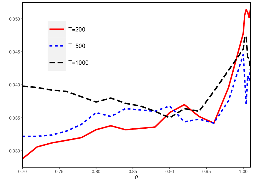
Following Nagakura 2009a, we employ three data generating mechanism to evaluate empirical sizes: (i) εt∼i.i.d​N​(0,1)\varepsilon_{t}\sim\mathrm{i.i.d}\ N(0,1), so that ψ=0\psi=0, (ii) εt∼i.i.d⁡(χ2​(10)−10)/20\varepsilon_{t}\sim\mathrm{i.i.d}\ (\chi^{2}(10)-10)/\sqrt{20}, so that ψ=0.5\psi=0.5, and (iii) εt∼i.i.d⁡(χ2​(1)−1)/2\varepsilon_{t}\sim\mathrm{i.i.d}\ (\chi^{2}(1)-1)/\sqrt{2}, so that ψ=0.756\psi=0.756. For each case, we set y0=0y_{0}=0. The sample size we use is T∈{200,500,1000}T\in\{200,500,1000\}, and the number of replications is 5,000. The ρT=ρ\rho_{T}=\rho values are fixed across TT, and we consider ρ∈[0.7,1.01]\rho\in[0.7,1.01]. The simulation results are collected in Figure 6. The general pattern is that the empirical rejection rates under H0H_{0} are relatively small when ρ<1\rho<1 and tend to be greater than the nominal level 0.05 when ρ\rho is near unity. As for the normal case (Figure 6(a)), rejection rates are stable around 0.05 over ρ∈[0.7,1.01]\rho\in[0.7,1.01], with them approaching 0.05 as TT increases. As for the chi square cases (Figure 6(b) and (c)), rejection rates stay around the nominal level, but they get farther away from 0.05 when |ψ||\psi| is larger, TT is smaller and ρ\rho is near 1. In particular, when εt∼i.i.d⁡(χ2​(1)−1)/2\varepsilon_{t}\sim\mathrm{i.i.d}\ (\chi^{2}(1)-1)/\sqrt{2} and T=200T=200, the rejection rates can be as large as 0.09 (around ρ=1\rho=1), although they approach 0.05 as TT increases. A similar tendency can be observed in the finite-sample behavior of modified LN tests proposed by Nagakura 2009a according to his simulation results. One possible cause of this phenomenon would be the finite-sample bias involved in the estimation of ψ\psi when the ψ\psi value is large. One may be advised to use a more conservative Bonferroni-Wald test (with smaller α1\alpha_{1} values) when the |ψ||\psi| estimate is large and the sample size is not so large.

4.2 Finite-sample power comparison

Next, we investigate tests’ ability to detect the nonzero variance in the autoregressive root. The simulation design is as follows: T=200T=200, εt∼i.i.d​N​(0,1)\varepsilon_{t}\sim\mathrm{i.i.d}\ N(0,1) and vt∼i.i.d​N​(0,1)v_{t}\sim\mathrm{i.i.d}\ N(0,1) with Corr⁡(εt,vt)∈{0,0.25,0.5,0.75}\mathrm{Corr}(\varepsilon_{t},v_{t})\in\{0,0.25,0.5,0.75\}, ρ∈{1.01,1,0.98,0.95}\rho\in\{1.01,1,0.98,0.95\}, and ω2∈(0,0.01]\omega^{2}\in(0,0.01] (corresponding to c2∈(0,28.28]c^{2}\in(0,28.28]). The tests we consider here are the Bonferroni-Wald test, the infeasible modified Wald test (calculated using the true ρ\rho), and one of the modified LN tests proposed by Nagakura 2009a, which is denoted by G~T,1\widetilde{G}_{T,1} in his notation. The infeasible Wald test is taken as a benchmark, and thereby we can evaluate the power loss originating from using the confidence interval for ρ\rho to perform the Bonferroni-Wald test. Nagakura 2009a’s modified LN test statistic is designed to converge in distribution under H0H_{0} to the standard normal irrespective of the ψ\psi value, under the data generating mechanism with ρ∈(−1,1]\rho\in(-1,1] fixed (i.e., independent of TT). Because Nagakura 2009a did not show its asymptotic null distribution remains standard normal when ρ>1\rho>1, we do not perform it for the case ρ=1.01\rho=1.01. We also consider the test proposed recently by Horváth and Trapani 2019 (hereafter HT). The HT test is a randomized one, and their test statistic ΘT,R\Theta_{T,R} (in their notation) converges in distribution to the chi square with one degree of freedom, for almost all realizations.88 8 The HT test needs a tuning parameter, x∈(0,0.5)x\in(0,0.5), to be performed, and they stated their test’s performance is insensitive to the choice of the xx value and set x=0.1x=0.1. However, in our simulation, their test’s performance is somehow affected by the choice of xx. Thus, we set x=0.38x=0.38, to obtain simulation results similar to those of HT. The HT test is not originally proposed under the local-to-unity specification, but it will be informative to practitioners to reveal the performance of the test under this setting.

The simulation results are shown in Figures 7 through 10. For the case ρ=1.01\rho=1.01, where all but the LN test are performed, the infeasible and Bonferroni-Wald tests have good power, and the discrepancy between their power functions is small. The latter result is due to the refinement on the construction of the confidence interval for ρ\rho. In contrast, the power function of the HT test stays around the nominal level 0.05 over ω2∈(0,0.01]\omega^{2}\in(0,0.01], which implies it has almost no distinguishing power for these alternatives. Indeed, HT conjectured (based on some theoretical analysis) that their test would have no power when 1−ρT=O⁡(T−1)1-\rho_{T}=O(T^{-1}) and ωT2=O⁡(T−1)\omega_{T}^{2}=O(T^{-1}), which is of larger magnitude than our local-to-zero variance ωT2=O(T−3/2)\omega_{T}^{2}=O(T^{-3/2}).99 9 Nishi and Kurozumi 2022 showed that under the STUR specification, the LN and some other tests are consistent when ωT2=O⁡(T−1)\omega_{T}^{2}=O(T^{-1}), from which they concluded that this case should be regarded as capturing stochastic “moderate” departures from a unit root rather than local departures. Our simulation results corroborate their statement.

Turning to the cases ρ≤1\rho\leq 1, it is noticeable that for each ρ\rho, the LN test performs well for small values of Corr⁡(εt,vt)\mathrm{Corr}(\varepsilon_{t},v_{t}), but Wald type tests outperform the LN test otherwise. In particular, the greater value of Corr⁡(εt,vt)\mathrm{Corr}(\varepsilon_{t},v_{t}) leads to the greater dominance by the Wald type tests. The power function of HT test, again, stays around the nominal level for these cases. Overall, the Bonferroni-Wald test performs better than the LN and HT tests for moderate to large values of Corr⁡(εt,vt)\mathrm{Corr}(\varepsilon_{t},v_{t}) (irrespective of the ρ\rho value) and performs almost as efficiently as its ideal, infeasible counterpart.

5 Empirical Application

In this section, we apply the Bonferroni-Wald test along with the LN and HT tests1010 10 Based on our simulation results, we set the tuning parameter x=0.38x=0.38 for the HT test. to several U.S. macroeconomic and financial time series, following Hill and Peng 2014 and HT. The dataset includes CPI, real GDP, industrial production, M2, S&P500, the 3 month Treasury bill rate and the unemployment rate. We take the logarithm of the first 5 series before detrending all the series. All data have been extracted from Federal Reserve Economic Data. The data description and testing results are displayed in Tables 2 and 3, respectively.

Before discussing main results, it should be recalled from our simulation results that the Bonferroni-Wald test can be oversized when TT is not large, ψ\psi is large and ρ\rho is near unity (see Section 4). Thus, we need to check whether all the three conditions hold for our series or not. According to Table 3, all the ρ\rho estimates are near unity, as expected. We also have obtained moderate estimates of ψ\psi for the CPI and S&P500 series, but the sample sizes for them are large enough that it is unlikely the Bonferroni-Wald test is oversized for these series. As for GDP, the sample size is T=292T=292 but the ψ\psi estimate is near zero, and hence we expect the Bonferroni-Wald test is not severely oversized for this series. Overall, all the three conditions for the potential oversize problem do not jointly hold.

For GDP and T-bill rate, we have obtained consistent results from all the three tests: the null of H0:ω2=0H_{0}:\omega^{2}=0 is not rejected for these series. This coincidence could be viewed as evidence for nonrandomness of the autoregressive root for these series. As for CPI, industrial production and S&P500, it is observed that the Bonferroni-Wald and LN tests reject the null while the HT test does not. This result will be attributed to the fact that the former two tests are much more powerful than the latter one. Finally, as for M2 and unemployment rate, only the Bonferroni-Wald test rejects the null. This outcome will be due to the fact that the Bonferroni-Wald test tends to be the most powerful among the three tests.

In Table 3, we also present the ω2\omega^{2} estimates proposed by Horváth and Trapani 2019 (denoted by ω^HT2\hat{\omega}^{2}_{\mathrm{HT}}). They showed this estimator is consistent under the non-local RCA models (with ρ\rho and ω2\omega^{2} fixed). The values of ω^HT2\hat{\omega}^{2}_{\mathrm{HT}} seem to support our testing results. For instance, we have a negative ω^HT2\hat{\omega}^{2}_{\mathrm{HT}} for T-bill rate, for which none of the tests reject the null. Moreover, for the other series, ω^HT2\hat{\omega}^{2}_{\mathrm{HT}} takes values around 10−410^{-4} to 10−310^{-3}, magnitudes of the coefficient randomness with which the HT test tends to be powerless under the sample size given in Table 3. For example, for M2, the sample size is T=2044T=2044, and ω^HT2\hat{\omega}^{2}_{\mathrm{HT}} is 3.12×10−43.12\times 10^{-4}, translating into c^2=ω^HT2×T3/2=28.83\hat{c}^{2}=\hat{\omega}^{2}_{\mathrm{HT}}\times T^{3/2}=28.83 estimate of the localizing coefficient c2c^{2}. According to our simulation results, the HT test has almost no power against the alternative of this magnitude, hence the testing result given in Table 3.

Given these findings, our empirical application illustrates the merit in choosing our Bonferroni-Wald test over existing ones.

6 Conclusion and Discussion

Given the results of empirical analyses conducted by earlier studies, the local-to-unity RCA models, which extend the STUR modelling, are empirically relevant. Under this setting, we can analyze the effect of the correlation between the random coefficient and disturbance on the power properties of tests for coefficient randomness. Theoretical and simulation analyses reveal that tests proposed by earlier studies can perform poorly when the degree of the correlation is moderate to large and the coefficient randomness is local to zero, while the augmented-Wald test we have proposed performs well even in such cases. Our test is also independent of the nuisance parameter ψ\psi, the correlation between the disturbance and its square, so that it is implementable without the knowledge about the value of ψ\psi. To deal with the uncertainty about the mean ρ\rho of the autoregressive root, we have proposed using a confidence interval for ρ\rho, leading to the Bonferroni-Wald test, where the significance level for the confidence interval is selected according to the value of the ψ\psi estimate. Embedding this selection process into the Bonferroni-Wald test helps stabilize the test’s size and improve the test’s power.

Several directions for future research are possible. First, from the similarity in the construction of test statistics between our model and predictive regressions, it is expected that the theory developed by numerous studies on predictive regressions can be applied to testing for coefficient randomness in local-to-unity autoregressions. For example Phillips and Lee 2013; Phillips and Lee 2016 proposed the use of the so-called IVX procedure for predictability testing (Kostakis et al. 2015, see also). This procedure leads to good size and power properties and also requires less computational burden for implementation than the Bonferroni approach employed by Campbell and Yogo 2006. The use of the IVX approach may facilitate testing for coefficient randomness in local-to-unity autoregressions. The analysis of tests’ performance when ρ\rho is distant from unity will also be of interest. In such a case, more preferable tests might be available than the Bonferroni-Wald test, which is based on the local-to-unity asymptotics.

References

  • (1)
  • Aue and Horváth (2011) Aue, A. and L. Horváth (2011) Quasi-Likelihood Estimation in Stationary and Nonstationary Autoregressive Models with Random Coefficients. Statistica Sinica, 21 (3), 973–999.
  • Campbell and Yogo (2006) Campbell, J. Y. and M. Yogo (2006) Efficient Tests of Stock Return Predictability. Journal of Financial Economics, 81 (1), 27–60.
  • Cavanagh et al. (1995) Cavanagh, C. L., G. Elliott, and J. H. Stock (1995) Inference in Models with Nearly Integrated Regressors. Econometric Theory, 11 (5), 1131–1147.
  • Distaso (2008) Distaso, W. (2008) Testing for Unit Root Processes in Random Coefficient Autoregressive Models. Journal of Econometrics, 142 (1), 581–609.
  • Elliott et al. (1996) Elliott, G., T. J. Rothenberg, and J. H. Stock (1996) Efficient Tests for an Autoregressive Unit Root. Econometrica, 64 (4), 813–836.
  • Hansen (1992) Hansen, B. E. (1992) Convergence to Stochastic Integrals for Dependent Heterogeneous Processes. Econometric Theory, 8 (4), 489–500.
  • Hill and Peng (2014) Hill, J. and L. Peng (2014) Unified Interval Estimation for Random Coefficient Autoregressive Models. Journal of Time Series Analysis, 35 (3), 282–297.
  • Horváth and Trapani (2019) Horváth, L. and L. Trapani (2019) Testing for Randomness in a Random Coefficient Autoregression Model. Journal of Econometrics, 209 (2), 338–352.
  • Horváth and Trapani (2022) Horváth, L. and L. Trapani (2022) Changepoint Detection in Heteroscedastic Random Coefficient Autoregressive Models. Journal of Business & Economic Statistics (forthcoming).
  • Hwang and Basawa (2005) Hwang, S. Y. and I. V. Basawa (2005) Explosive Random-Coefficient AR(1) Processes and Related Asymptotics for Least-Squares Estimation. Journal of Time Series Analysis, 26 (6), 807–824.
  • Kostakis et al. (2015) Kostakis, A., T. Magdalinos, and M. P. Stamatogiannis (2015) Robust Econometric Inference for Stock Return Predictability. The Review of Financial Studies, 28 (5), 1506–1553.
  • Lee (1998) Lee, S. (1998) Coefficient Constancy Test in a Random Coefficient Autoregressive Model. Journal of Statistical Planning and Inference, 74 (1), 93–101.
  • Leybourne et al. (1996) Leybourne, S. J., B. P. M. McCabe, and A. R. Tremayne (1996) Can Economic Time Series Be Differenced to Stationarity? Journal of business & economic statistics, 14 (4), 435.
  • McCabe and Smith (1998) McCabe, B. P. M. and R. J. Smith (1998) The Power of Some Tests for Difference Stationarity under Local Heteroscedastic Integration. Journal of the American Statistical Association, 93 (442), 751–761.
  • McCabe and Tremayne (1995) McCabe, B. P. M. and A. R. Tremayne (1995) Testing a Time Series for Difference Stationarity. The Annals of Statistics, 23 (3), 1015–1028.
  • Nagakura (2009a) Nagakura, D. (2009a) Testing for Coefficient Stability of AR(1) Model When the Null Is an Integrated or a Stationary Process. Journal of Statistical Planning and Inference, 139 (8), 2731–2745.
  • Nagakura (2009b) Nagakura, D. (2009b) Asymptotic Theory for Explosive Random Coefficient Autoregressive Models and Inconsistency of a Unit Root Test against a Stochastic Unit Root Process. Statistics & Probability Letters, 79 (24), 2476–2483.
  • Nicholls and Quinn (1982) Nicholls, D. F. and B. G. Quinn (1982) Random Coefficient Autoregressive Models: An Introduction, 11 of Lecture Notes in Statistics, New York, NY Springer US.
  • Nishi and Kurozumi (2022) Nishi, M. and E. Kurozumi (2022) Stochastic Local and Moderate Departures from a Unit Root and Its Application to Unit Root Testing.Technical Report 2022-02, Graduate School of Economics, Hitotsubashi University.
  • Phillips (1987) Phillips, P. C. B. (1987) Towards a Unified Asymptotic Theory for Autoregression. Biometrika, 74 (3), 535–547.
  • Phillips (2014) Phillips, P. C. B. (2014) On Confidence Intervals for Autoregressive Roots and Predictive Regression. Econometrica, 82 (3), 1177–1195.
  • Phillips and Lee (2013) Phillips, P. C. B. and J. H. Lee (2013) Predictive Regression under Various Degrees of Persistence and Robust Long-Horizon Regression. Journal of Econometrics, 177 (2), 250–264.
  • Phillips and Lee (2016) Phillips, P. C. B. and J. H. Lee (2016) Robust Econometric Inference with Mixed Integrated and Mildly Explosive Regressors. Journal of Econometrics, 192 (2), 433–450.
  • Phillips and Ouliaris (1990) Phillips, P. C. B. and S. Ouliaris (1990) Asymptotic Properties of Residual Based Tests for Cointegration. Econometrica, 58 (1), 165–193.
  • Stock (1991) Stock, J. H. (1991) Confidence Intervals for the Largest Autoregressive Root in U.S. Macroeconomic Time Series. Journal of Monetary Economics, 28 (3), 435–459.
  • Su and Roca (2012) Su, J.-J. and E. Roca (2012) Examining the Power of Stochastic Unit Root Tests without Assuming Independence in the Error Processes of the Underlying Time Series. Applied Economics Letters, 19 (4), 373–377.

Appendix A: Procedure to Determine α1\alpha_{1} Values for the Bonferroni-Wald Test

In this appendix, we describe the procedure to determine the α1\alpha_{1} values for the confidence interval for ρT\rho_{T} explained in Section 3. The procedure is based on simulating asymptotic distributions with 5,000 replications. In each replication, we first generate {yt}t=1T\{y_{t}\}_{t=1}^{T} by the mechanism

yt=(1+a/T)yt−1+εt,t=1,2,…,T\displaystyle y_{t}=(1+a/T)y_{t-1}+\varepsilon_{t},\quad t=1,2,\ldots,T (A.1)

with y0=0y_{0}=0, T=2000T=2000, a∈[−300,10]a\in[-300,10] and εt∼i.i.d​N​(0,1)\varepsilon_{t}\sim\mathrm{i.i.d}\ N(0,1). Then, with given α1\alpha_{1}, we conduct the two-step procedure for the Bonferroni-Wald test explained in Section 3 and calculate the frequency of H0H_{0} being rejected for the α1\alpha_{1}.

Note that εt\varepsilon_{t} used in (A.1) satisfies ψ=Corr⁡(εt,εt2−σε2)=0\psi=\mathrm{Corr}(\varepsilon_{t},\varepsilon_{t}^{2}-\sigma_{\varepsilon}^{2})=0. To calculate the false rejection frequencies for other ψ\psi values, we artificially produce an environment where the Wald test statistic depends on ψ≠0\psi\neq 0. Noting that under the null,

zt2​(ρ¯T)=1+(εt2−1)+(a¯/T−a/T)2​yt−12−2​(a¯/T−a/T)​yt−1​εt,\displaystyle z_{t}^{2}(\bar{\rho}_{T})=1+(\varepsilon_{t}^{2}-1)+(\bar{a}/T-a/T)^{2}y_{t-1}^{2}-2(\bar{a}/T-a/T)y_{t-1}\varepsilon_{t},

and ηt=εt2−1\eta_{t}=\varepsilon_{t}^{2}-1 (combined with εt\varepsilon_{t}) determines the value of ψ\psi on which the asymptotic distribution of WT∗​(ρ¯T)W_{T}^{*}(\bar{\rho}_{T}) depends, we artificially replace ηt=εt2−1\eta_{t}=\varepsilon_{t}^{2}-1 with ηtr​e​p≔1−ψ2​ηt+ψ​2​εt\eta_{t}^{rep}\coloneqq\sqrt{1-\psi^{2}}\eta_{t}+\psi\sqrt{2}\varepsilon_{t}, obtaining

zt2​(ρ¯T)r​e​p\displaystyle z_{t}^{2}(\bar{\rho}_{T})^{rep} ≔1+ηtr​e​p+(a¯/T−a/T)2​yt−12−2​(a¯/T−a/T)​yt−1​εt,\displaystyle\coloneqq 1+\eta_{t}^{rep}+(\bar{a}/T-a/T)^{2}y_{t-1}^{2}-2(\bar{a}/T-a/T)y_{t-1}\varepsilon_{t},

in view of the distributional equivalence Wη=d1−ψ2​W1+ψ​WεW_{\eta}\stackrel{{\scriptstyle d}}{{=}}\sqrt{1-\psi^{2}}W_{1}+\psi W_{\varepsilon} and the fact that 𝕍⁡[ηt]=ση2=2\mathbb{V}[\eta_{t}]=\sigma_{\eta}^{2}=2 and Corr⁡(ηt,εt)=0\mathrm{Corr}(\eta_{t},\varepsilon_{t})=0. In this replacement, the newly crafted variable ηtr​e​p\eta_{t}^{rep} takes over the role of ηt=εt2−1\eta_{t}=\varepsilon_{t}^{2}-1, satisfying 𝔼⁡[ηtr​e​p]=0\mathbb{E}[\eta_{t}^{rep}]=0, 𝕍⁡[ηtr​e​p]=2=𝕍⁡[ηt]\mathbb{V}[\eta_{t}^{rep}]=2=\mathbb{V}[\eta_{t}] and Corr⁡(ηtr​e​p,εt)=ψ\mathrm{Corr}(\eta_{t}^{rep},\varepsilon_{t})=\psi by construction. This replacement can be justified by the fact that under the null, the Wald test statistic asymptotically depends only on ψ\psi (and aa) and is not dependent on any other moment. It follows that the Bonferroni-Wald test statistic using zt2​(ρ¯T)r​e​pz_{t}^{2}(\bar{\rho}_{T})^{rep} in place of zt2​(ρ¯T)z_{t}^{2}(\bar{\rho}_{T}) asymptotically depends on ψ\psi, so that we can calculate the false rejection frequencies for any value of ψ\psi.

For each ψ\psi on some grid, we calculate the false rejection rates of the Bonferroni-Wald test with aa moving over a grid on [−300,10][-300,10] and determine the value of α1\alpha_{1} for the given ψ\psi such that the false rejection rate is less than or equal to 0.05 for all aa.

Appendix B: Proofs of Results in Section 2

In this appendix, we prove the theorems stated in Section 2.

Lemma B.1.

Consider model (2) under Assumptions 1 and 2. Define the stochastic process YTY_{T} on [0,1][0,1] by YT(r)≔T−1/2y⌊T​r⌋, 0≤r≤1Y_{T}(r)\coloneqq T^{-1/2}y_{\lfloor Tr\rfloor},\ 0\leq r\leq 1. Then, YT⇒σε​JaY_{T}\Rightarrow\sigma_{\varepsilon}J_{a} in the Skorokhod space D⁡[0,1]D[0,1], where JaJ_{a} solves d​Ja​(r)=a​Ja​(r)​d​r+d​Wε​(r)dJ_{a}(r)=aJ_{a}(r)dr+dW_{\varepsilon}(r).

Proof. The proof is essentially the same as that of Lemma 1(a) of Nishi and Kurozumi 2022 and hence is omitted. ∎

Lemma B.2.

Consider model (2) under Assumptions 1 and 2. Then, we have

  • (a)

    σ^ε,T2​(ρT)→pσε2\hat{\sigma}_{\varepsilon,T}^{2}(\rho_{T})\stackrel{{\scriptstyle p}}{{\to}}\sigma_{\varepsilon}^{2},

  • (b)

    σ^η,T2​(ρT)→pση2\hat{\sigma}_{\eta,T}^{2}(\rho_{T})\stackrel{{\scriptstyle p}}{{\to}}\sigma_{\eta}^{2},

  • (c)

    ψ^T​(ρT)→pψ\hat{\psi}_{T}(\rho_{T})\stackrel{{\scriptstyle p}}{{\to}}\psi.

Proof. The proofs of parts (a) and (b) are identical to those of Lemma 1(b) and (c) of Nishi and Kurozumi 2022 and hence are omitted. To prove part (c), it suffices to show

T−1​∑t=1Tzt​(ρT)​{zt2​(ρT)−σ^ε,T2​(ρT)}→p𝔼⁡[εt3].\displaystyle T^{-1}\sum_{t=1}^{T}z_{t}(\rho_{T})\Big\{z_{t}^{2}(\rho_{T})-\hat{\sigma}_{\varepsilon,T}^{2}(\rho_{T})\Bigr\}\stackrel{{\scriptstyle p}}{{\to}}\mathbb{E}[\varepsilon_{t}^{3}].

A simple calculation gives

T−1​∑t=1Tzt​(ρT)​{zt2​(ρT)−σ^ε,T2​(ρT)}\displaystyle T^{-1}\sum_{t=1}^{T}z_{t}(\rho_{T})\{z_{t}^{2}(\rho_{T})-\hat{\sigma}_{\varepsilon,T}^{2}(\rho_{T})\}
=T−1∑t=1T(cT−3/4yt−1vt+εt){c2T−3/2yt−12vt2+2cT−3/4yt−1εtvt+εt2−σ^ε,T2(ρT)}\displaystyle=T^{-1}\sum_{t=1}^{T}(cT^{-3/4}y_{t-1}v_{t}+\varepsilon_{t})\{c^{2}T^{-3/2}y_{t-1}^{2}v_{t}^{2}+2cT^{-3/4}y_{t-1}\varepsilon_{t}v_{t}+\varepsilon_{t}^{2}-\hat{\sigma}_{\varepsilon,T}^{2}(\rho_{T})\}
=T−1​∑t=1Tεt3+AT,\displaystyle=T^{-1}\sum_{t=1}^{T}\varepsilon_{t}^{3}+A_{T},

where

AT≔c3T−13/4∑t=1Tyt−13vt3\displaystyle A_{T}\coloneqq c^{3}T^{-13/4}\sum_{t=1}^{T}y_{t-1}^{3}v_{t}^{3} +3c2T−5/2∑t=1Tyt−12εtvt2+3cT−7/4∑t=1Tyt−1εt2vt\displaystyle+3c^{2}T^{-5/2}\sum_{t=1}^{T}y_{t-1}^{2}\varepsilon_{t}v_{t}^{2}+3cT^{-7/4}\sum_{t=1}^{T}y_{t-1}\varepsilon_{t}^{2}v_{t}
−σ^ε,T2(ρT)×{cT−7/4∑t=1Tyt−1vt+T−1∑t=1Tεt}.\displaystyle-\hat{\sigma}_{\varepsilon,T}^{2}(\rho_{T})\times\Bigl\{cT^{-7/4}\sum_{t=1}^{T}y_{t-1}v_{t}+T^{-1}\sum_{t=1}^{T}\varepsilon_{t}\Bigr\}.

The first term of ATA_{T} satisfies

c3T−13/4∑t=1Tyt−13vt3\displaystyle c^{3}T^{-13/4}\sum_{t=1}^{T}y_{t-1}^{3}v_{t}^{3} =c3𝔼[vt3]T−13/4∑t=1Tyt−13+c3T−13/4∑t=1Tyt−13(vt3−𝔼[vt3])\displaystyle=c^{3}\mathbb{E}[v_{t}^{3}]T^{-13/4}\sum_{t=1}^{T}y_{t-1}^{3}+c^{3}T^{-13/4}\sum_{t=1}^{T}y_{t-1}^{3}(v_{t}^{3}-\mathbb{E}[v_{t}^{3}])
=c3𝔼[vt3]T−3/4∫01YT3(r)dr+c3T−5/4∫01YT3(r)dWv3−𝔼⁡[v3],T(r)=Op(T−3/4),\displaystyle=c^{3}\mathbb{E}[v_{t}^{3}]T^{-3/4}\int_{0}^{1}Y_{T}^{3}(r)dr+c^{3}T^{-5/4}\int_{0}^{1}Y_{T}^{3}(r)dW_{v^{3}-\mathbb{E}[v^{3}],T}(r)=O_{p}(T^{-3/4}),

say, because {vt3−𝔼⁡[vt3]}\{v_{t}^{3}-\mathbb{E}[v_{t}^{3}]\} is i.i.d with zero mean and finite variance. Similarly, we can prove that the other terms of ATA_{T} is Op(T−1/4)O_{p}(T^{-1/4}). Thus

T−1​∑t=1Tzt​(ρT)​{zt2​(ρT)−σ^ε,T2​(ρT)}=T−1​∑t=1Tεt3+op​(1)→p𝔼⁡[εt3].\displaystyle T^{-1}\sum_{t=1}^{T}z_{t}(\rho_{T})\{z_{t}^{2}(\rho_{T})-\hat{\sigma}_{\varepsilon,T}^{2}(\rho_{T})\}=T^{-1}\sum_{t=1}^{T}\varepsilon_{t}^{3}+o_{p}(1)\stackrel{{\scriptstyle p}}{{\to}}\mathbb{E}[\varepsilon_{t}^{3}].

∎

For later reference, we give several results on the weak convergence of components of test statistics.

Lemma B.3.

Consider model (2) under Assumptions 1 and 2. Then, we have

  • (a)
    T−3/2∑t=1Tyt−12~zt2(ρT)⇒σησε2∫01Ja,2~(r)dWη(r)+c2σε4∫01(Ja,2~)2(r)dr+2cσε4q∫01Ja,1~(r)Ja,2~(r)dr,\displaystyle T^{-3/2}\sum_{t=1}^{T}\widetilde{y_{t-1}^{2}}z_{t}^{2}(\rho_{T})\Rightarrow\sigma_{\eta}\sigma_{\varepsilon}^{2}\int_{0}^{1}\widetilde{J_{a,2}}(r)dW_{\eta}(r)+c^{2}\sigma_{\varepsilon}^{4}\int_{0}^{1}(\widetilde{J_{a,2}})^{2}(r)dr+2c\sigma_{\varepsilon}^{4}q\int_{0}^{1}\widetilde{J_{a,1}}(r)\widetilde{J_{a,2}}(r)dr,
  • (b)
    T−1​∑t=1Tyt−1~​zt2​(ρT)⇒ση​σε​∫01Ja,1~​(r)​d​Wη​(r)+c2​σε3​∫01Ja,1~​(r)​Ja,2~​(r)​𝑑r+2​c​σε3​q​∫01(Ja,1~)2​(r)​𝑑r.\displaystyle T^{-1}\sum_{t=1}^{T}\widetilde{y_{t-1}}z_{t}^{2}(\rho_{T})\Rightarrow\sigma_{\eta}\sigma_{\varepsilon}\int_{0}^{1}\widetilde{J_{a,1}}(r)dW_{\eta}(r)+c^{2}\sigma_{\varepsilon}^{3}\int_{0}^{1}\widetilde{J_{a,1}}(r)\widetilde{J_{a,2}}(r)dr+2c\sigma_{\varepsilon}^{3}q\int_{0}^{1}(\widetilde{J_{a,1}})^{2}(r)dr.
  • (c)

    σ^ξ∗~2​(ρT)→pση2\hat{\sigma}_{\widetilde{\xi^{*}}}^{2}(\rho_{T})\stackrel{{\scriptstyle p}}{{\to}}\sigma_{\eta}^{2},

  • (d)

    σ^ξ∗⁣∗~2​(ρT)→pση2\hat{\sigma}_{\widetilde{\xi^{**}}}^{2}(\rho_{T})\stackrel{{\scriptstyle p}}{{\to}}\sigma_{\eta}^{2},

where σ^ξ∗~2​(ρT)\hat{\sigma}_{\widetilde{\xi^{*}}}^{2}(\rho_{T}) and σ^ξ∗⁣∗~2​(ρT)\hat{\sigma}_{\widetilde{\xi^{**}}}^{2}(\rho_{T}) are the OLS variance estimators of (8) and (13), respectively.

Proof. For part (a), a straightforward calculation gives

T−3/2∑t=1Tyt−12~zt2(ρT)=B1,T+B2,T+B3,T,\displaystyle T^{-3/2}\sum_{t=1}^{T}\widetilde{y_{t-1}^{2}}z_{t}^{2}(\rho_{T})=B_{1,T}+B_{2,T}+B_{3,T},

where

B1,T\displaystyle B_{1,T} ≔T−3/2∑t=1T(yt−12−T−1∑t=1Tyt−12)(εt2−σε2),\displaystyle\coloneqq T^{-3/2}\sum_{t=1}^{T}\Bigl(y_{t-1}^{2}-T^{-1}\sum_{t=1}^{T}y_{t-1}^{2}\Bigr)(\varepsilon_{t}^{2}-\sigma_{\varepsilon}^{2}),
B2,T\displaystyle B_{2,T} ≔c2​T−3​∑t=1T(yt−12−T−1​∑t=1Tyt−12)​yt−12​vt2,\displaystyle\coloneqq c^{2}T^{-3}\sum_{t=1}^{T}\Bigl(y_{t-1}^{2}-T^{-1}\sum_{t=1}^{T}y_{t-1}^{2}\Bigr)y_{t-1}^{2}v_{t}^{2},
and
B3,T\displaystyle B_{3,T} ≔2cT−9/4∑t=1T(yt−12−T−1∑t=1Tyt−12)yt−1εtvt.\displaystyle\coloneqq 2cT^{-9/4}\sum_{t=1}^{T}\Bigl(y_{t-1}^{2}-T^{-1}\sum_{t=1}^{T}y_{t-1}^{2}\Bigr)y_{t-1}\varepsilon_{t}v_{t}.

It is straightforward to show B1,T⇒ση​σε2​∫01Ja,2~​(r)​d​Wη​(r)B_{1,T}\Rightarrow\sigma_{\eta}\sigma_{\varepsilon}^{2}\int_{0}^{1}\widetilde{J_{a,2}}(r)dW_{\eta}(r), using Lemma B.1 and Theorem 2.1 of Hansen 1992. As for B2,TB_{2,T}, we have

B2,T\displaystyle B_{2,T} =c2​T−3​∑t=1T(yt−12−T−1​∑t=1Tyt−12)2+c2​T−3​∑t=1T(yt−12−T−1​∑t=1Tyt−12)​yt−12​(vt2−1)\displaystyle=c^{2}T^{-3}\sum_{t=1}^{T}\Bigl(y_{t-1}^{2}-T^{-1}\sum_{t=1}^{T}y_{t-1}^{2}\Bigr)^{2}+c^{2}T^{-3}\sum_{t=1}^{T}\Bigl(y_{t-1}^{2}-T^{-1}\sum_{t=1}^{T}y_{t-1}^{2}\Bigr)y_{t-1}^{2}(v_{t}^{2}-1)
=c2∫01(YT2(r)−∫01YT2(s)ds)2dr+c2T−1/2∫01(YT2(r)−∫01YT2(s)ds)YT2(r)dWv2−1,T\displaystyle=c^{2}\int_{0}^{1}\Bigl(Y_{T}^{2}(r)-\int_{0}^{1}Y_{T}^{2}(s)ds\Bigr)^{2}dr+c^{2}T^{-1/2}\int_{0}^{1}\Bigl(Y_{T}^{2}(r)-\int_{0}^{1}Y_{T}^{2}(s)ds\Bigr)Y_{T}^{2}(r)dW_{v^{2}-1,T}
⇒c2​σε4​∫01(Ja,2~)2​(r)​𝑑r,\displaystyle\Rightarrow c^{2}\sigma_{\varepsilon}^{4}\int_{0}^{1}(\widetilde{J_{a,2}})^{2}(r)dr,

where the last convergence follows from Lemma B.1 and the continuous mapping theorem (CMT). By a similar argument, we obtain

B3,T\displaystyle B_{3,T} =2cσεqT−5/2∑t=1T(yt−12−T−1∑t=1Tyt−12)(yt−1−T−1∑t=1Tyt−1)\displaystyle=2c\sigma_{\varepsilon}qT^{-5/2}\sum_{t=1}^{T}\Bigl(y_{t-1}^{2}-T^{-1}\sum_{t=1}^{T}y_{t-1}^{2}\Bigr)\Bigl(y_{t-1}-T^{-1}\sum_{t=1}^{T}y_{t-1}\Bigr)
+2cT−9/4∑t=1T(yt−12−T−1∑t=1Tyt−12)yt−1(εtvt−σε​v)\displaystyle+2cT^{-9/4}\sum_{t=1}^{T}\Bigl(y_{t-1}^{2}-T^{-1}\sum_{t=1}^{T}y_{t-1}^{2}\Bigr)y_{t-1}(\varepsilon_{t}v_{t}-\sigma_{\varepsilon v})
⇒2​c​σε4​q​∫01Ja,2~​(r)​Ja,1~​(r)​𝑑r.\displaystyle\Rightarrow 2c\sigma_{\varepsilon}^{4}q\int_{0}^{1}\widetilde{J_{a,2}}(r)\widetilde{J_{a,1}}(r)dr.

Therefore, we arrive at

T−3/2∑t=1Tyt−12~zt2(ρT)⇒σησε2∫01Ja,2~(r)dWη(r)+c2σε4∫01(Ja,2~)2(r)dr+2cσε4q∫01Ja,2~(r)Ja,1~(r)dr,\displaystyle T^{-3/2}\sum_{t=1}^{T}\widetilde{y_{t-1}^{2}}z_{t}^{2}(\rho_{T})\Rightarrow\sigma_{\eta}\sigma_{\varepsilon}^{2}\int_{0}^{1}\widetilde{J_{a,2}}(r)dW_{\eta}(r)+c^{2}\sigma_{\varepsilon}^{4}\int_{0}^{1}(\widetilde{J_{a,2}})^{2}(r)dr+2c\sigma_{\varepsilon}^{4}q\int_{0}^{1}\widetilde{J_{a,2}}(r)\widetilde{J_{a,1}}(r)dr,

as desired.

Part (b) can be proven in a similar fashion. Write T−1​∑t=1Tyt−1~​zt2​(ρT)T^{-1}\sum_{t=1}^{T}\widetilde{y_{t-1}}z_{t}^{2}(\rho_{T}) as

T−1​∑t=1Tyt−1~​zt2​(ρT)=C1,T+C2,T+C3,T,\displaystyle T^{-1}\sum_{t=1}^{T}\widetilde{y_{t-1}}z_{t}^{2}(\rho_{T})=C_{1,T}+C_{2,T}+C_{3,T},

where C1,T≔T−1​∑t=1Tyt−1~​(εt2−σε2)C_{1,T}\coloneqq T^{-1}\sum_{t=1}^{T}\widetilde{y_{t-1}}(\varepsilon_{t}^{2}-\sigma_{\varepsilon}^{2}), C2,T≔c2​T−52​∑t=1Tyt−1~​yt−12​vt2C_{2,T}\coloneqq c^{2}T^{-\frac{5}{2}}\sum_{t=1}^{T}\widetilde{y_{t-1}}y_{t-1}^{2}v_{t}^{2}, and C3,T≔2​c​T−74​∑t=1Tyt−1~​yt−1​εt​vtC_{3,T}\coloneqq 2cT^{-\frac{7}{4}}\sum_{t=1}^{T}\widetilde{y_{t-1}}y_{t-1}\varepsilon_{t}v_{t}. Then, it is straightforward to show

C1,T\displaystyle C_{1,T} ⇒ση​σε​∫01Ja,1~​(r)​d​Wη​(r),\displaystyle\Rightarrow\sigma_{\eta}\sigma_{\varepsilon}\int_{0}^{1}\widetilde{J_{a,1}}(r)dW_{\eta}(r),
C2,T\displaystyle C_{2,T} ⇒c2​σε3​∫01Ja,1~​(r)​Ja,2~​(r)​𝑑r,\displaystyle\Rightarrow c^{2}\sigma_{\varepsilon}^{3}\int_{0}^{1}\widetilde{J_{a,1}}(r)\widetilde{J_{a,2}}(r)dr,
and
C3,T\displaystyle C_{3,T} ⇒2​c​σε3​q​∫01(Ja,1~)2​(r)​𝑑r.\displaystyle\Rightarrow 2c\sigma_{\varepsilon}^{3}q\int_{0}^{1}(\widetilde{J_{a,1}})^{2}(r)dr.

Combining the above results completes the proof of part (b).

To prove part (c), we define M≔IT−X~​(X~′​X~)−1​X~M\coloneqq I_{T}-\widetilde{X}(\widetilde{X}^{\prime}\widetilde{X})^{-1}\widetilde{X} and write σ^ξ∗~2​(ρT)\hat{\sigma}_{\widetilde{\xi^{*}}}^{2}(\rho_{T}) as

σ^ξ∗~2​(ρT)\displaystyle\hat{\sigma}_{\widetilde{\xi^{*}}}^{2}(\rho_{T}) =T−1​Ξ∗~′​M​Ξ∗~\displaystyle=T^{-1}\widetilde{\Xi^{*}}^{\prime}M\widetilde{\Xi^{*}}
=T−1​∑t=1T(ξt∗~)2−T−1​(∑t=1Tyt−1~​ξt∗∑t=1Tyt−12~​ξt∗)\displaystyle=T^{-1}\sum_{t=1}^{T}(\widetilde{\xi^{*}_{t}})^{2}-T^{-1}\begin{pmatrix}\sum_{t=1}^{T}\widetilde{y_{t-1}}\xi_{t}^{*}&\sum_{t=1}^{T}\widetilde{y_{t-1}^{2}}\xi_{t}^{*}\\ \end{pmatrix}
×(∑t=1T(yt−1~)2∑t=1Tyt−1~​yt−12~∑t=1Tyt−12~​yt−1~∑t=1T(yt−12~)2)−1​(∑t=1Tyt−1~​ξt∗∑t=1Tyt−12~​ξt∗).\displaystyle\times\begin{pmatrix}\sum_{t=1}^{T}(\widetilde{y_{t-1}})^{2}&\sum_{t=1}^{T}\widetilde{y_{t-1}}\widetilde{y_{t-1}^{2}}\\ \sum_{t=1}^{T}\widetilde{y_{t-1}^{2}}\widetilde{y_{t-1}}&\sum_{t=1}^{T}(\widetilde{y_{t-1}^{2}})^{2}\\ \end{pmatrix}^{-1}\begin{pmatrix}\sum_{t=1}^{T}\widetilde{y_{t-1}}\xi_{t}^{*}\\ \sum_{t=1}^{T}\widetilde{y_{t-1}^{2}}\xi_{t}^{*}\\ \end{pmatrix}. (B.1)

The first term of (B.1) becomes

T−1​∑t=1T(ξt∗~)2\displaystyle T^{-1}\sum_{t=1}^{T}(\widetilde{\xi_{t}^{*}})^{2} =T−1​∑t=1T(ξt∗)2−(T−1​∑t=1Tξt∗)2\displaystyle=T^{-1}\sum_{t=1}^{T}(\xi_{t}^{*})^{2}-\Bigl(T^{-1}\sum_{t=1}^{T}\xi_{t}^{*}\Bigr)^{2}
=T−1∑t=1T{c2T−3/2yt−12(vt2−1)+2cT−3/4yt−1(εtvt−σε​v)+(εt2−σε2)}2\displaystyle=T^{-1}\sum_{t=1}^{T}\{c^{2}T^{-3/2}y_{t-1}^{2}(v_{t}^{2}-1)+2cT^{-3/4}y_{t-1}(\varepsilon_{t}v_{t}-\sigma_{\varepsilon v})+(\varepsilon_{t}^{2}-\sigma_{\varepsilon}^{2})\}^{2}
−[T−1∑t=1T{c2T−3/2yt−12(vt2−1)+2cT−3/4yt−1(εtvt−σε​v)+(εt2−σε2)}]2\displaystyle-\Bigl[T^{-1}\sum_{t=1}^{T}\{c^{2}T^{-3/2}y_{t-1}^{2}(v_{t}^{2}-1)+2cT^{-3/4}y_{t-1}(\varepsilon_{t}v_{t}-\sigma_{\varepsilon v})+(\varepsilon_{t}^{2}-\sigma_{\varepsilon}^{2})\}\Bigr]^{2}
=T−1​∑t=1T(εt2−σε2)2+op​(1)\displaystyle=T^{-1}\sum_{t=1}^{T}(\varepsilon_{t}^{2}-\sigma_{\varepsilon}^{2})^{2}+o_{p}(1)
→pση2.\displaystyle\stackrel{{\scriptstyle p}}{{\to}}\sigma_{\eta}^{2}.

The second term of (B.1) satisfies

T−1​(∑t=1Tyt−1~​ξt∗∑t=1Tyt−12~​ξt∗)​(∑t=1T(yt−1~)2∑t=1Tyt−1~​yt−12~∑t=1Tyt−12~​yt−1~∑t=1T(yt−12~)2)−1​(∑t=1Tyt−1~​ξt∗∑t=1Tyt−12~​ξt∗)\displaystyle T^{-1}\begin{pmatrix}\sum_{t=1}^{T}\widetilde{y_{t-1}}\xi_{t}^{*}&\sum_{t=1}^{T}\widetilde{y_{t-1}^{2}}\xi_{t}^{*}\\ \end{pmatrix}\begin{pmatrix}\sum_{t=1}^{T}(\widetilde{y_{t-1}})^{2}&\sum_{t=1}^{T}\widetilde{y_{t-1}}\widetilde{y_{t-1}^{2}}\\ \sum_{t=1}^{T}\widetilde{y_{t-1}^{2}}\widetilde{y_{t-1}}&\sum_{t=1}^{T}(\widetilde{y_{t-1}^{2}})^{2}\\ \end{pmatrix}^{-1}\begin{pmatrix}\sum_{t=1}^{T}\widetilde{y_{t-1}}\xi_{t}^{*}\\ \sum_{t=1}^{T}\widetilde{y_{t-1}^{2}}\xi_{t}^{*}\\ \end{pmatrix}
=T−1​(T−1​∑t=1Tyt−1~​(εt2−σε2)+op​(1)T−3/2∑t=1Tyt−12~(εt2−σε2)+op(1))\displaystyle=T^{-1}\begin{pmatrix}T^{-1}\sum_{t=1}^{T}\widetilde{y_{t-1}}(\varepsilon_{t}^{2}-\sigma_{\varepsilon}^{2})+o_{p}(1)&T^{-3/2}\sum_{t=1}^{T}\widetilde{y_{t-1}^{2}}(\varepsilon_{t}^{2}-\sigma_{\varepsilon}^{2})+o_{p}(1)\\ \end{pmatrix}
×(T−2​∑t=1T(yt−1~)2T−5/2∑t=1Tyt−1~yt−12~T−5/2∑t=1Tyt−12~yt−1~T−3​∑t=1T(yt−12~)2)−1​(T−1​∑t=1Tyt−1~​(εt2−σε2)+op​(1)T−3/2∑t=1Tyt−12~(εt2−σε2)+op(1))\displaystyle\times\begin{pmatrix}T^{-2}\sum_{t=1}^{T}(\widetilde{y_{t-1}})^{2}&T^{-5/2}\sum_{t=1}^{T}\widetilde{y_{t-1}}\widetilde{y_{t-1}^{2}}\\ T^{-5/2}\sum_{t=1}^{T}\widetilde{y_{t-1}^{2}}\widetilde{y_{t-1}}&T^{-3}\sum_{t=1}^{T}(\widetilde{y_{t-1}^{2}})^{2}\\ \end{pmatrix}^{-1}\begin{pmatrix}T^{-1}\sum_{t=1}^{T}\widetilde{y_{t-1}}(\varepsilon_{t}^{2}-\sigma_{\varepsilon}^{2})+o_{p}(1)\\ T^{-3/2}\sum_{t=1}^{T}\widetilde{y_{t-1}^{2}}(\varepsilon_{t}^{2}-\sigma_{\varepsilon}^{2})+o_{p}(1)\\ \end{pmatrix}
=Op​(T−1).\displaystyle=O_{p}(T^{-1}). (B.2)

Hence, we obtain σ^ξ∗~2​(ρT)→pση2\hat{\sigma}_{\widetilde{\xi^{*}}}^{2}(\rho_{T})\stackrel{{\scriptstyle p}}{{\to}}\sigma_{\eta}^{2}, as desired.

To prove part (d), let Z1~≔(z1~​(ρT),z2~​(ρT),…,zT~​(ρT))′\widetilde{Z_{1}}\coloneqq(\widetilde{z_{1}}(\rho_{T}),\widetilde{z_{2}}(\rho_{T}),\ldots,\widetilde{z_{T}}(\rho_{T}))^{\prime}. Then, Z2∗~​(ρT)\widetilde{Z_{2}^{*}}(\rho_{T}) is expressed as

Z2∗~​(ρT)=11−ψ^T2​(ρT)​{Z2~​(ρT)−σ^η,T​(ρT)​ψ^T​(ρT)σ^ε,T​(ρT)​Z1~​(ρT)},\displaystyle\widetilde{Z_{2}^{*}}(\rho_{T})=\frac{1}{\sqrt{1-\hat{\psi}_{T}^{2}(\rho_{T})}}\Bigl\{\widetilde{Z_{2}}(\rho_{T})-\frac{\hat{\sigma}_{\eta,T}(\rho_{T})\hat{\psi}_{T}(\rho_{T})}{\hat{\sigma}_{\varepsilon,T}(\rho_{T})}\widetilde{Z_{1}}(\rho_{T})\Bigr\},

which yields

σ^ξ∗⁣∗~2=T−1​Z2∗~​(ρT)′​M​Z2∗~​(ρT)=11−ψ^T2​(ρT)​{D1,T−2​σ^η,T​(ρT)​ψ^T​(ρT)σ^ε,T​(ρT)​D2,T+σ^η,T2​(ρT)​ψ^T2​(ρT)σ^ε,T2​(ρT)​D3,T},\displaystyle\hat{\sigma}_{\widetilde{\xi^{**}}}^{2}=T^{-1}\widetilde{Z_{2}^{*}}(\rho_{T})^{\prime}M\widetilde{Z_{2}^{*}}(\rho_{T})=\frac{1}{1-\hat{\psi}_{T}^{2}(\rho_{T})}\Bigl\{D_{1,T}-2\frac{\hat{\sigma}_{\eta,T}(\rho_{T})\hat{\psi}_{T}(\rho_{T})}{\hat{\sigma}_{\varepsilon,T}(\rho_{T})}D_{2,T}+\frac{\hat{\sigma}_{\eta,T}^{2}(\rho_{T})\hat{\psi}_{T}^{2}(\rho_{T})}{\hat{\sigma}_{\varepsilon,T}^{2}(\rho_{T})}D_{3,T}\Bigr\}, (B.3)

where D1,T≔T−1​Z2~​(ρT)′​M​Z2~​(ρT)D_{1,T}\coloneqq T^{-1}\widetilde{Z_{2}}(\rho_{T})^{\prime}M\widetilde{Z_{2}}(\rho_{T}), D2,T≔T−1​Z2~​(ρT)′​M​Z1~​(ρT)D_{2,T}\coloneqq T^{-1}\widetilde{Z_{2}}(\rho_{T})^{\prime}M\widetilde{Z_{1}}(\rho_{T}), and D3,T≔T−1​Z1~​(ρT)′​M​Z1~​(ρT)D_{3,T}\coloneqq T^{-1}\widetilde{Z_{1}}(\rho_{T})^{\prime}M\widetilde{Z_{1}}(\rho_{T}). Since D1,TD_{1,T} is σ^ξ∗~2​(ρT)\hat{\sigma}_{\widetilde{\xi^{*}}}^{2}(\rho_{T}), we have already proven in part (c) that

D1,T→pση2.\displaystyle D_{1,T}\stackrel{{\scriptstyle p}}{{\to}}\sigma_{\eta}^{2}. (B.4)

In view of equation (8), D2,TD_{2,T} becomes

D2,T\displaystyle D_{2,T} =T−1​Ξ∗~​(ρT)′​M​Z1~​(ρT)\displaystyle=T^{-1}\widetilde{\Xi^{*}}(\rho_{T})^{\prime}M\widetilde{Z_{1}}(\rho_{T})
=T−1​∑t=1Tξt∗​zt~​(ρT)−T−1​(∑t=1Tyt−1~​ξt∗∑t=1Tyt−12~​ξt∗)\displaystyle=T^{-1}\sum_{t=1}^{T}\xi_{t}^{*}\widetilde{z_{t}}(\rho_{T})-T^{-1}\begin{pmatrix}\sum_{t=1}^{T}\widetilde{y_{t-1}}\xi_{t}^{*}&\sum_{t=1}^{T}\widetilde{y_{t-1}^{2}}\xi_{t}^{*}\\ \end{pmatrix}
×(∑t=1T(yt−1~)2∑t=1Tyt−1~​yt−12~∑t=1Tyt−12~​yt−1~∑t=1T(yt−12~)2)−1​(∑t=1Tyt−1~​zt​(ρT)∑t=1Tyt−12~​zt​(ρT)).\displaystyle\ \ \ \times\begin{pmatrix}\sum_{t=1}^{T}(\widetilde{y_{t-1}})^{2}&\sum_{t=1}^{T}\widetilde{y_{t-1}}\widetilde{y_{t-1}^{2}}\\ \sum_{t=1}^{T}\widetilde{y_{t-1}^{2}}\widetilde{y_{t-1}}&\sum_{t=1}^{T}(\widetilde{y_{t-1}^{2}})^{2}\end{pmatrix}^{-1}\begin{pmatrix}\sum_{t=1}^{T}\widetilde{y_{t-1}}z_{t}(\rho_{T})\\ \sum_{t=1}^{T}\widetilde{y_{t-1}^{2}}z_{t}(\rho_{T})\\ \end{pmatrix}.

As for the first term of D2,TD_{2,T}, we have

T−1​∑t=1Tξt∗​zt~​(ρT)\displaystyle T^{-1}\sum_{t=1}^{T}\xi_{t}^{*}\widetilde{z_{t}}(\rho_{T}) =T−1∑t=1T{c2T−3/2yt−12(vt2−1)+2cT−3/4yt−1(εtvt−σε​v)+(εt2−σε2)}\displaystyle=T^{-1}\sum_{t=1}^{T}\{c^{2}T^{-3/2}y_{t-1}^{2}(v_{t}^{2}-1)+2cT^{-3/4}y_{t-1}(\varepsilon_{t}v_{t}-\sigma_{\varepsilon v})+(\varepsilon_{t}^{2}-\sigma_{\varepsilon}^{2})\}
×(zt​(ρT)−T−1​∑t=1Tzt​(ρT))\displaystyle\ \ \ \ \ \ \times\Bigl(z_{t}(\rho_{T})-T^{-1}\sum_{t=1}^{T}z_{t}(\rho_{T})\Bigr)
=T−1​∑t=1T(εt2−σε2)​εt+op​(1)→p𝔼⁡[εt3].\displaystyle=T^{-1}\sum_{t=1}^{T}(\varepsilon_{t}^{2}-\sigma_{\varepsilon}^{2})\varepsilon_{t}+o_{p}(1)\stackrel{{\scriptstyle p}}{{\to}}\mathbb{E}[\varepsilon_{t}^{3}].

We can also show that the second term of D2,TD_{2,T} is Op​(T−1)O_{p}(T^{-1}) in the same way as we did in (B.2). Thus, we get

D2,T→p𝔼⁡[εt3].\displaystyle D_{2,T}\stackrel{{\scriptstyle p}}{{\to}}\mathbb{E}[\varepsilon_{t}^{3}]. (B.5)

Lastly, D3,TD_{3,T} becomes

D3,T\displaystyle D_{3,T} =T−1​Z1~​(ρT)′​M​Z1~​(ρT)\displaystyle=T^{-1}\widetilde{Z_{1}}(\rho_{T})^{\prime}M\widetilde{Z_{1}}(\rho_{T})
=T−1​∑t=1Tzt~2​(ρT)−T−1​(∑t=1Tyt−1~​zt​(ρT)∑t=1Tyt−12~​zt​(ρT))′\displaystyle=T^{-1}\sum_{t=1}^{T}\widetilde{z_{t}}^{2}(\rho_{T})-T^{-1}\begin{pmatrix}\sum_{t=1}^{T}\widetilde{y_{t-1}}z_{t}(\rho_{T})&\sum_{t=1}^{T}\widetilde{y_{t-1}^{2}}z_{t}(\rho_{T})\\ \end{pmatrix}^{\prime}
×(∑t=1T(yt−1~)2∑t=1Tyt−1~​yt−12~∑t=1Tyt−12~​yt−1~∑t=1T(yt−12~)2)−1​(∑t=1Tyt−1~​zt​(ρT)∑t=1Tyt−12~​zt​(ρT))\displaystyle\ \ \ \ \ \ \ \ \ \ \ \times\begin{pmatrix}\sum_{t=1}^{T}(\widetilde{y_{t-1}})^{2}&\sum_{t=1}^{T}\widetilde{y_{t-1}}\widetilde{y_{t-1}^{2}}\\ \sum_{t=1}^{T}\widetilde{y_{t-1}^{2}}\widetilde{y_{t-1}}&\sum_{t=1}^{T}(\widetilde{y_{t-1}^{2}})^{2}\\ \end{pmatrix}^{-1}\begin{pmatrix}\sum_{t=1}^{T}\widetilde{y_{t-1}}z_{t}(\rho_{T})\\ \sum_{t=1}^{T}\widetilde{y_{t-1}^{2}}z_{t}(\rho_{T})\\ \end{pmatrix}
=σ^ε,T2​(ρT)−(T−1​∑t=1Tzt​(ρT))2+Op​(T−1)→pσε2.\displaystyle=\hat{\sigma}_{\varepsilon,T}^{2}(\rho_{T})-\Bigl(T^{-1}\sum_{t=1}^{T}z_{t}(\rho_{T})\Bigr)^{2}+O_{p}(T^{-1})\stackrel{{\scriptstyle p}}{{\to}}\sigma_{\varepsilon}^{2}. (B.6)

Substituting (B.4) through (B.6) into (B.3) and applying Lemma B.2, we deduce

σ^ξ∗⁣∗~2\displaystyle\hat{\sigma}_{\widetilde{\xi^{**}}}^{2} →p11−ψ2​{ση2−2​ση​ψσε​𝔼​[εt3]+ση2​ψ2σε2​σε2}\displaystyle\stackrel{{\scriptstyle p}}{{\to}}\frac{1}{1-\psi^{2}}\Bigl\{\sigma_{\eta}^{2}-2\frac{\sigma_{\eta}\psi}{\sigma_{\varepsilon}}\mathbb{E}[\varepsilon_{t}^{3}]+\frac{\sigma_{\eta}^{2}\psi^{2}}{\sigma_{\varepsilon}^{2}}\sigma_{\varepsilon}^{2}\Bigr\}
=11−ψ2​(ση2−2​ση2​ψ2+ση2​ψ2)=ση2.\displaystyle=\frac{1}{1-\psi^{2}}(\sigma_{\eta}^{2}-2\sigma_{\eta}^{2}\psi^{2}+\sigma_{\eta}^{2}\psi^{2})=\sigma_{\eta}^{2}.

∎

Proof of Theorem 1. First, note that

LNT​(ρT)=T−3/2∑t=1Tyt−12~zt2(ρT)σ^η,T​(ρT)​{T−3​∑t=1T(yt−12~)2}1/2.\displaystyle\mathrm{LN}_{T}(\rho_{T})=\frac{T^{-3/2}\sum_{t=1}^{T}\widetilde{y_{t-1}^{2}}z_{t}^{2}(\rho_{T})}{\hat{\sigma}_{\eta,T}(\rho_{T})\Bigl\{T^{-3}\sum_{t=1}^{T}(\widetilde{y_{t-1}^{2}})^{2}\Bigr\}^{1/2}}.

Then, using Lemmas B.2 and B.3 and the CMT, we deduce

LNT​(ρT)\displaystyle\mathrm{LN}_{T}(\rho_{T}) ⇒ση​σε2​∫01Ja,2~​(r)​d​Wη​(r)+c2​σε4​∫01(Ja,2~)2​(r)​𝑑r+2​c​σε4​q​∫01Ja,1~​(r)​Ja,2~​(r)​𝑑rση​{σε4​∫01(Ja,2~)2​(r)​𝑑r}1/2\displaystyle\Rightarrow\frac{\sigma_{\eta}\sigma_{\varepsilon}^{2}\int_{0}^{1}\widetilde{J_{a,2}}(r)dW_{\eta}(r)+c^{2}\sigma_{\varepsilon}^{4}\int_{0}^{1}(\widetilde{J_{a,2}})^{2}(r)dr+2c\sigma_{\varepsilon}^{4}q\int_{0}^{1}\widetilde{J_{a,1}}(r)\widetilde{J_{a,2}}(r)dr}{\sigma_{\eta}\Bigl\{\sigma_{\varepsilon}^{4}\int_{0}^{1}(\widetilde{J_{a,2}})^{2}(r)dr\Bigr\}^{1/2}}
=∫01Ja,2~​(r)​d​Wη​(r){∫01(Ja,2~)2​(r)​𝑑r}1/2+σε2ση​[c2​∫01(Ja,2~)2​(r)​𝑑r+2​c​q​∫01Ja,2~​(r)​Ja,1~​(r)​𝑑r{∫01(Ja,2~)2​(r)​𝑑r}1/2].\displaystyle=\frac{\int_{0}^{1}\widetilde{J_{a,2}}(r)dW_{\eta}(r)}{\bigl\{\int_{0}^{1}\bigl(\widetilde{J_{a,2}}\bigr)^{2}(r)dr\bigr\}^{1/2}}+\frac{\sigma_{\varepsilon}^{2}}{\sigma_{\eta}}\Biggl[\frac{c^{2}\int_{0}^{1}\bigl(\widetilde{J_{a,2}}\bigr)^{2}(r)dr+2cq\int_{0}^{1}\widetilde{J_{a,2}}(r)\widetilde{J_{a,1}}(r)dr}{\bigl\{\int_{0}^{1}\bigl(\widetilde{J_{a,2}}\bigr)^{2}(r)dr\bigr\}^{1/2}}\Biggr].

∎

Proof of Theorem 2. First, by Lemma B.3(c) and the CMT, the denominator of tω^T2​(ρT)t_{\hat{\omega}_{T}^{2}}(\rho_{T}) divided by T3/2T^{3/2} becomes

σ^ξ∗~(ρT)T−3/2(X2~′M1X2~)1/2\displaystyle\hat{\sigma}_{\widetilde{\xi^{*}}}(\rho_{T})T^{-3/2}(\widetilde{X_{2}}^{\prime}M_{1}\widetilde{X_{2}})^{1/2} =σ^ξ∗~​(ρT)​{T−3​(M1​X2~)′​(M1​X2~)}1/2\displaystyle=\hat{\sigma}_{\widetilde{\xi^{*}}}(\rho_{T})\{T^{-3}(M_{1}\widetilde{X_{2}})^{\prime}(M_{1}\widetilde{X_{2}})\}^{1/2}
=σ^ξ∗~​(ρT)​{T−3​∑t=1T(yt−12~−∑t=1Tyt−1~​yt−12~∑t=1T(yt−1~)2​yt−1~)2}1/2\displaystyle=\hat{\sigma}_{\widetilde{\xi^{*}}}(\rho_{T})\biggl\{T^{-3}\sum_{t=1}^{T}\Bigl(\widetilde{y_{t-1}^{2}}-\frac{\sum_{t=1}^{T}\widetilde{y_{t-1}}\widetilde{y_{t-1}^{2}}}{\sum_{t=1}^{T}(\widetilde{y_{t-1}})^{2}}\widetilde{y_{t-1}}\Bigr)^{2}\biggr\}^{1/2}
=σ^ξ∗~​(ρT)​{∫01(Y2,T~​(r)−∫01Y1,T~​(s)​Y2,T~​(s)​𝑑s∫01(Y1,T~)2​(s)​𝑑s​Y1,T~​(r))2}1/2\displaystyle=\hat{\sigma}_{\widetilde{\xi^{*}}}(\rho_{T})\biggl\{\int_{0}^{1}\Bigl(\widetilde{Y_{2,T}}(r)-\frac{\int_{0}^{1}\widetilde{Y_{1,T}}(s)\widetilde{Y_{2,T}}(s)ds}{\int_{0}^{1}(\widetilde{Y_{1,T}})^{2}(s)ds}\widetilde{Y_{1,T}}(r)\Bigr)^{2}\biggr\}^{1/2}
⇒ση​{σε4​∫01(Ja,2~​(r)−∫01Ja,1~​(s)​Ja,2~​(s)​𝑑s∫01(Ja,1~)2​(s)​𝑑s​Ja,1~​(r))2​𝑑r}1/2\displaystyle\Rightarrow\sigma_{\eta}\biggl\{\sigma_{\varepsilon}^{4}\int_{0}^{1}\Bigl(\widetilde{J_{a,2}}(r)-\frac{\int_{0}^{1}\widetilde{J_{a,1}}(s)\widetilde{J_{a,2}}(s)ds}{\int_{0}^{1}(\widetilde{J_{a,1}})^{2}(s)ds}\widetilde{J_{a,1}}(r)\Bigr)^{2}dr\biggr\}^{1/2}
=ση​σε2​[∫01Qa2​(r)​𝑑r]1/2,\displaystyle=\sigma_{\eta}\sigma_{\varepsilon}^{2}\Bigl[\int_{0}^{1}Q_{a}^{2}(r)dr\Bigr]^{1/2},

where Y1,T~​(r)≔YT​(r)−∫01YT​(s)​𝑑s\widetilde{Y_{1,T}}(r)\coloneqq Y_{T}(r)-\int_{0}^{1}Y_{T}(s)ds and Y2,T~​(r)≔YT2​(r)−∫01YT2​(s)​𝑑s\widetilde{Y_{2,T}}(r)\coloneqq Y_{T}^{2}(r)-\int_{0}^{1}Y_{T}^{2}(s)ds. Next, applying Lemma B.3, the numerator of tω^T2​(ρT)t_{\hat{\omega}_{T}^{2}}(\rho_{T}) divided by T3/2T^{3/2} is seen to satisfy

T−3/2X2~′M1Z2~(ρT)\displaystyle T^{-3/2}\widetilde{X_{2}}^{\prime}M_{1}\widetilde{Z_{2}}(\rho_{T}) =T−3/2∑t=1Tyt−12~zt2(ρT)−T−5/2∑t=1Tyt−1~yt−12~T−1∑t=1Tyt−1~zt2(ρT)T−2​∑t=1T(yt−1~)2\displaystyle=T^{-3/2}\sum_{t=1}^{T}\widetilde{y_{t-1}^{2}}z_{t}^{2}(\rho_{T})-\frac{T^{-5/2}\sum_{t=1}^{T}\widetilde{y_{t-1}}\widetilde{y_{t-1}^{2}}T^{-1}\sum_{t=1}^{T}\widetilde{y_{t-1}}z_{t}^{2}(\rho_{T})}{T^{-2}\sum_{t=1}^{T}(\widetilde{y_{t-1}})^{2}}
⇒ση​σε2​∫01Ja,2~​(r)​d​Wη​(r)+c2​σε4​∫01(Ja,2~)2​(r)​𝑑r+2​c​σε4​q​∫01Ja,1~​(r)​Ja,2~​(r)​𝑑r\displaystyle\Rightarrow\sigma_{\eta}\sigma_{\varepsilon}^{2}\int_{0}^{1}\widetilde{J_{a,2}}(r)dW_{\eta}(r)+c^{2}\sigma_{\varepsilon}^{4}\int_{0}^{1}(\widetilde{J_{a,2}})^{2}(r)dr+2c\sigma_{\varepsilon}^{4}q\int_{0}^{1}\widetilde{J_{a,1}}(r)\widetilde{J_{a,2}}(r)dr
−σε3∫01Ja,1~(r)Ja,2~(r)dr\displaystyle-\sigma_{\varepsilon}^{3}\int_{0}^{1}\widetilde{J_{a,1}}(r)\widetilde{J_{a,2}}(r)dr
×ση​σε​∫01Ja,1~​(r)​d​Wη​(r)+c2​σε3​∫01Ja,1~​(r)​Ja,2~​(r)​𝑑r+2​c​σε3​q​∫01(Ja,1~)2​(r)​𝑑rσε2​∫01(Ja,1~)2​(r)​𝑑r\displaystyle\times\frac{\sigma_{\eta}\sigma_{\varepsilon}\int_{0}^{1}\widetilde{J_{a,1}}(r)dW_{\eta}(r)+c^{2}\sigma_{\varepsilon}^{3}\int_{0}^{1}\widetilde{J_{a,1}}(r)\widetilde{J_{a,2}}(r)dr+2c\sigma_{\varepsilon}^{3}q\int_{0}^{1}(\widetilde{J_{a,1}})^{2}(r)dr}{\sigma_{\varepsilon}^{2}\int_{0}^{1}(\widetilde{J_{a,1}})^{2}(r)dr}
=ση​σε2​∫01Qa​(r)​d​Wη​(r)+c2​σε4​∫01Qa2​(r)​𝑑r.\displaystyle=\sigma_{\eta}\sigma_{\varepsilon}^{2}\int_{0}^{1}Q_{a}(r)dW_{\eta}(r)+c^{2}\sigma_{\varepsilon}^{4}\int_{0}^{1}Q_{a}^{2}(r)dr.

Combining the above results gives

tω^T2​(ρT)⇒∫01Qa​(r)​d​Wη​(r)[∫01Qa2​(r)​𝑑r]1/2+c2​σε2ση​[∫01Qa2​(r)​𝑑r]1/2.\displaystyle t_{\hat{\omega}_{T}^{2}}(\rho_{T})\Rightarrow\frac{\int_{0}^{1}Q_{a}(r)dW_{\eta}(r)}{\bigl[\int_{0}^{1}Q_{a}^{2}(r)dr\bigr]^{1/2}}+\frac{c^{2}\sigma_{\varepsilon}^{2}}{\sigma_{\eta}}\Biggl[\int_{0}^{1}Q_{a}^{2}(r)dr\Biggr]^{1/2}.

To derive the asymptotic distribution of WT​(ρT)W_{T}(\rho_{T}), note that

WT​(ρT)\displaystyle W_{T}(\rho_{T}) =σ^ξ∗~−2​(X~′​Z2~​(ρT))′​(X~′​X~)−1​(X~′​Z2~​(ρT))\displaystyle=\hat{\sigma}_{\widetilde{\xi^{*}}}^{-2}(\widetilde{X}^{\prime}\widetilde{Z_{2}}(\rho_{T}))^{\prime}(\widetilde{X}^{\prime}\widetilde{X})^{-1}(\widetilde{X}^{\prime}\widetilde{Z_{2}}(\rho_{T}))
=σ^ξ∗~−2​(T−1​∑t=1Tyt−1~​zt2​(ρT)T−3/2∑t=1Tyt−12~zt2(ρT))′​(T−2​∑t=1T(yt−1~)2T−5/2∑t=1Tyt−1~yt−12~T−5/2∑t=1Tyt−12~yt−1~T−3​∑t=1T(yt−12~)2)−1\displaystyle=\hat{\sigma}_{\widetilde{\xi^{*}}}^{-2}\begin{pmatrix}T^{-1}\sum_{t=1}^{T}\widetilde{y_{t-1}}z_{t}^{2}(\rho_{T})\\ T^{-3/2}\sum_{t=1}^{T}\widetilde{y_{t-1}^{2}}z_{t}^{2}(\rho_{T})\\ \end{pmatrix}^{\prime}\begin{pmatrix}T^{-2}\sum_{t=1}^{T}(\widetilde{y_{t-1}})^{2}&T^{-5/2}\sum_{t=1}^{T}\widetilde{y_{t-1}}\widetilde{y_{t-1}^{2}}\\ T^{-5/2}\sum_{t=1}^{T}\widetilde{y_{t-1}^{2}}\widetilde{y_{t-1}}&T^{-3}\sum_{t=1}^{T}(\widetilde{y_{t-1}^{2}})^{2}\\ \end{pmatrix}^{-1}
×(T−1​∑t=1Tyt−1~​zt2​(ρT)T−3/2∑t=1Tyt−12~zt2(ρT)).\displaystyle\ \ \ \ \ \ \ \ \ \ \ \times\begin{pmatrix}T^{-1}\sum_{t=1}^{T}\widetilde{y_{t-1}}z_{t}^{2}(\rho_{T})\\ T^{-3/2}\sum_{t=1}^{T}\widetilde{y_{t-1}^{2}}z_{t}^{2}(\rho_{T})\\ \end{pmatrix}.

Then, applying Lemma B.3 and the CMT, we get

WT​(ρT)\displaystyle W_{T}(\rho_{T}) ⇒ση−2​(ση​σε​∫01Ja,1~​(r)​d​Wη​(r)+c2​σε3​∫01Ja,1~​(r)​Ja,2~​(r)​𝑑r+2​c​σε3​q​∫01(Ja,1~)2​(r)​𝑑rση​σε2​∫01Ja,2~​(r)​d​Wη​(r)+c2​σε4​∫01(Ja,2~)2​(r)​𝑑r+2​c​σε4​q​∫01Ja,1~​(r)​Ja,2~​(r)​𝑑r)′\displaystyle\Rightarrow\sigma_{\eta}^{-2}\begin{pmatrix}\sigma_{\eta}\sigma_{\varepsilon}\int_{0}^{1}\widetilde{J_{a,1}}(r)dW_{\eta}(r)+c^{2}\sigma_{\varepsilon}^{3}\int_{0}^{1}\widetilde{J_{a,1}}(r)\widetilde{J_{a,2}}(r)dr+2c\sigma_{\varepsilon}^{3}q\int_{0}^{1}(\widetilde{J_{a,1}})^{2}(r)dr\\ \sigma_{\eta}\sigma_{\varepsilon}^{2}\int_{0}^{1}\widetilde{J_{a,2}}(r)dW_{\eta}(r)+c^{2}\sigma_{\varepsilon}^{4}\int_{0}^{1}(\widetilde{J_{a,2}})^{2}(r)dr+2c\sigma_{\varepsilon}^{4}q\int_{0}^{1}\widetilde{J_{a,1}}(r)\widetilde{J_{a,2}}(r)dr\\ \end{pmatrix}^{\prime}
×(σε2​∫01(Ja,1~)2​(r)​𝑑rσε3​∫01Ja,1~​(r)​Ja,2~​(r)​𝑑rσε3​∫01Ja,2~​(r)​Ja,1~​(r)​𝑑rσε4​∫01(Ja,2~)2​(r)​𝑑r)−1\displaystyle\times\begin{pmatrix}\sigma_{\varepsilon}^{2}\int_{0}^{1}\bigl(\widetilde{J_{a,1}}\bigr)^{2}(r)dr&\sigma_{\varepsilon}^{3}\int_{0}^{1}\widetilde{J_{a,1}}(r)\widetilde{J_{a,2}}(r)dr\\ \sigma_{\varepsilon}^{3}\int_{0}^{1}\widetilde{J_{a,2}}(r)\widetilde{J_{a,1}}(r)dr&\sigma_{\varepsilon}^{4}\int_{0}^{1}\bigl(\widetilde{J_{a,2}}\bigr)^{2}(r)dr\\ \end{pmatrix}^{-1}
×(ση​σε​∫01Ja,1~​(r)​d​Wη​(r)+c2​σε3​∫01Ja,1~​(r)​Ja,2~​(r)​𝑑r+2​c​σε3​q​∫01(Ja,1~)2​(r)​𝑑rση​σε2​∫01Ja,2~​(r)​d​Wη​(r)+c2​σε4​∫01(Ja,2~)2​(r)​𝑑r+2​c​σε4​q​∫01Ja,1~​(r)​Ja,2~​(r)​𝑑r)\displaystyle\times\begin{pmatrix}\sigma_{\eta}\sigma_{\varepsilon}\int_{0}^{1}\widetilde{J_{a,1}}(r)dW_{\eta}(r)+c^{2}\sigma_{\varepsilon}^{3}\int_{0}^{1}\widetilde{J_{a,1}}(r)\widetilde{J_{a,2}}(r)dr+2c\sigma_{\varepsilon}^{3}q\int_{0}^{1}(\widetilde{J_{a,1}})^{2}(r)dr\\ \sigma_{\eta}\sigma_{\varepsilon}^{2}\int_{0}^{1}\widetilde{J_{a,2}}(r)dW_{\eta}(r)+c^{2}\sigma_{\varepsilon}^{4}\int_{0}^{1}(\widetilde{J_{a,2}})^{2}(r)dr+2c\sigma_{\varepsilon}^{4}q\int_{0}^{1}\widetilde{J_{a,1}}(r)\widetilde{J_{a,2}}(r)dr\\ \end{pmatrix}
={(∫01Ja,1~​(r)​d​Wη​(r)∫01Ja,2~​(r)​d​Wη​(r))+σε2ση​(c2​∫01Ja,1~​(r)​Ja,2~​(r)​𝑑r+2​c​q​∫01(Ja,1~)2​(r)​𝑑rc2​∫01(Ja,2~)2​(r)​𝑑r+2​c​q​∫01Ja,1~​(r)​Ja,2~​(r)​𝑑r)}′\displaystyle=\Bigg\{\begin{pmatrix}\int_{0}^{1}\widetilde{J_{a,1}}(r)dW_{\eta}(r)\\ \int_{0}^{1}\widetilde{J_{a,2}}(r)dW_{\eta}(r)\end{pmatrix}+\frac{\sigma_{\varepsilon}^{2}}{\sigma_{\eta}}\begin{pmatrix}c^{2}\int_{0}^{1}\widetilde{J_{a,1}}(r)\widetilde{J_{a,2}}(r)dr+2cq\int_{0}^{1}\bigl(\widetilde{J_{a,1}}\bigr)^{2}(r)dr\\ c^{2}\int_{0}^{1}\bigl(\widetilde{J_{a,2}}\bigr)^{2}(r)dr+2cq\int_{0}^{1}\widetilde{J_{a,1}}(r)\widetilde{J_{a,2}}(r)dr\end{pmatrix}\Biggr\}^{\prime}
×(∫01(Ja,1~)2​(r)​𝑑r∫01Ja,1~​(r)​Ja,2~​(r)​𝑑r∫01Ja,2~​(r)​Ja,1~​(r)​𝑑r∫01(Ja,2~)2​(r)​𝑑r)−1\displaystyle\times\begin{pmatrix}\int_{0}^{1}\bigl(\widetilde{J_{a,1}}\bigr)^{2}(r)dr&\int_{0}^{1}\widetilde{J_{a,1}}(r)\widetilde{J_{a,2}}(r)dr\\ \int_{0}^{1}\widetilde{J_{a,2}}(r)\widetilde{J_{a,1}}(r)dr&\int_{0}^{1}\bigl(\widetilde{J_{a,2}}\bigr)^{2}(r)dr\end{pmatrix}^{-1}
×{(∫01Ja,1~​(r)​d​Wη​(r)∫01Ja,2~​(r)​d​Wη​(r))+σε2ση​(c2​∫01Ja,1~​(r)​Ja,2~​(r)​𝑑r+2​c​q​∫01(Ja,1~)2​(r)​𝑑rc2​∫01(Ja,2~)2​(r)​𝑑r+2​c​q​∫01Ja,1~​(r)​Ja,2~​(r)​𝑑r)},\displaystyle\times\Bigg\{\begin{pmatrix}\int_{0}^{1}\widetilde{J_{a,1}}(r)dW_{\eta}(r)\\ \int_{0}^{1}\widetilde{J_{a,2}}(r)dW_{\eta}(r)\end{pmatrix}+\frac{\sigma_{\varepsilon}^{2}}{\sigma_{\eta}}\begin{pmatrix}c^{2}\int_{0}^{1}\widetilde{J_{a,1}}(r)\widetilde{J_{a,2}}(r)dr+2cq\int_{0}^{1}\bigl(\widetilde{J_{a,1}}\bigr)^{2}(r)dr\\ c^{2}\int_{0}^{1}\bigl(\widetilde{J_{a,2}}\bigr)^{2}(r)dr+2cq\int_{0}^{1}\widetilde{J_{a,1}}(r)\widetilde{J_{a,2}}(r)dr\end{pmatrix}\Biggr\},

completing the proof. ∎

To prove Theorem 3, we use the following lemma.

Lemma B.4.

Consider model (2) under Assumptions 1 and 2. Then, we have

  • (a)
    T−3/2∑t=1Tyt−12~zt2∗(ρT)⇒\displaystyle T^{-3/2}\sum_{t=1}^{T}\widetilde{y_{t-1}^{2}}z_{t}^{2*}(\rho_{T})\Rightarrow ση​σε2​∫01Ja,2~​(r)​d​W1​(r)\displaystyle\sigma_{\eta}\sigma_{\varepsilon}^{2}\int_{0}^{1}\widetilde{J_{a,2}}(r)dW_{1}(r)
    +(1−ψ2)−1/2{c2σε4∫01(Ja,2~)2(r)dr+2cσε4q∫01Ja,1~(r)Ja,2~(r)dr},\displaystyle+(1-\psi^{2})^{-1/2}\Bigl\{c^{2}\sigma_{\varepsilon}^{4}\int_{0}^{1}(\widetilde{J_{a,2}})^{2}(r)dr+2c\sigma_{\varepsilon}^{4}q\int_{0}^{1}\widetilde{J_{a,1}}(r)\widetilde{J_{a,2}}(r)dr\Bigr\},
  • (b)
    T−1∑t=1Tyt−1~zt2∗(ρT)⇒\displaystyle T^{-1}\sum_{t=1}^{T}\widetilde{y_{t-1}}z_{t}^{2*}(\rho_{T})\Rightarrow ση​σε​∫01Ja,1~​(r)​d​W1​(r)\displaystyle\sigma_{\eta}\sigma_{\varepsilon}\int_{0}^{1}\widetilde{J_{a,1}}(r)dW_{1}(r)
    +(1−ψ2)−1/2{c2σε3∫01Ja,1~(r)Ja,2~(r)dr+2cσε3q∫01(Ja,1~)2(r)dr}.\displaystyle+(1-\psi^{2})^{-1/2}\Bigl\{c^{2}\sigma_{\varepsilon}^{3}\int_{0}^{1}\widetilde{J_{a,1}}(r)\widetilde{J_{a,2}}(r)dr+2c\sigma_{\varepsilon}^{3}q\int_{0}^{1}(\widetilde{J_{a,1}})^{2}(r)dr\Bigr\}.

Proof. To prove part (a), note that

T−3/2∑t=1Tyt−12~zt2∗(ρT)=11−ψ^T2​(ρT){E1,T−σ^η,T​(ρT)​ψ^T​(ρT)σ^ε,T​(ρT)E2,T},\displaystyle T^{-3/2}\sum_{t=1}^{T}\widetilde{y_{t-1}^{2}}z_{t}^{2*}(\rho_{T})=\frac{1}{\sqrt{1-\hat{\psi}_{T}^{2}(\rho_{T})}}\Bigl\{E_{1,T}-\frac{\hat{\sigma}_{\eta,T}(\rho_{T})\hat{\psi}_{T}(\rho_{T})}{\hat{\sigma}_{\varepsilon,T}(\rho_{T})}E_{2,T}\Bigr\},

where E1,T≔T−3/2∑t=1Tyt−12~zt2(ρT)E_{1,T}\coloneqq T^{-3/2}\sum_{t=1}^{T}\widetilde{y_{t-1}^{2}}z_{t}^{2}(\rho_{T}) and E2,T≔T−3/2∑t=1Tyt−12~zt(ρT)E_{2,T}\coloneqq T^{-3/2}\sum_{t=1}^{T}\widetilde{y_{t-1}^{2}}z_{t}(\rho_{T}). By Lemma B.3(a), E1,TE_{1,T} satisfies

E1,T⇒ση​σε2​∫01Ja,2~​(r)​d​Wη​(r)+c2​σε4​∫01(Ja,2~)2​(r)​𝑑r+2​c​σε4​q​∫01Ja,1~​(r)​Ja,2~​(r)​𝑑r.\displaystyle E_{1,T}\Rightarrow\sigma_{\eta}\sigma_{\varepsilon}^{2}\int_{0}^{1}\widetilde{J_{a,2}}(r)dW_{\eta}(r)+c^{2}\sigma_{\varepsilon}^{4}\int_{0}^{1}(\widetilde{J_{a,2}})^{2}(r)dr+2c\sigma_{\varepsilon}^{4}q\int_{0}^{1}\widetilde{J_{a,1}}(r)\widetilde{J_{a,2}}(r)dr.

As for E2,TE_{2,T}, a straightforward calculation yields

E2,T\displaystyle E_{2,T} =T−3/2∑t=1Tyt−12~(cT−3/4yt−1vt+εt)\displaystyle=T^{-3/2}\sum_{t=1}^{T}\widetilde{y_{t-1}^{2}}(cT^{-3/4}y_{t-1}v_{t}+\varepsilon_{t})
=T−3/2∑t=1Tyt−12~εt+Op(T−1/4)⇒σε3∫01Ja,2~(r)dWε(r).\displaystyle=T^{-3/2}\sum_{t=1}^{T}\widetilde{y_{t-1}^{2}}\varepsilon_{t}+O_{p}(T^{-1/4})\Rightarrow\sigma_{\varepsilon}^{3}\int_{0}^{1}\widetilde{J_{a,2}}(r)dW_{\varepsilon}(r).

Hence, we obtain

T−3/2∑t=1Tyt−12~zt2∗(ρT)\displaystyle T^{-3/2}\sum_{t=1}^{T}\widetilde{y_{t-1}^{2}}z_{t}^{2*}(\rho_{T}) ⇒11−ψ2{σησε2∫01Ja,2~(r)dWη(r)+c2σε4∫01(Ja,2~)2(r)dr\displaystyle\Rightarrow\frac{1}{\sqrt{1-\psi^{2}}}\biggl\{\sigma_{\eta}\sigma_{\varepsilon}^{2}\int_{0}^{1}\widetilde{J_{a,2}}(r)dW_{\eta}(r)+c^{2}\sigma_{\varepsilon}^{4}\int_{0}^{1}(\widetilde{J_{a,2}})^{2}(r)dr
+2cσε4q∫01Ja,1~(r)Ja,2~(r)dr−ση​ψσεσε3∫01Ja,2~(r)dWε(r)}\displaystyle\ \ \ \ \ \ \ +2c\sigma_{\varepsilon}^{4}q\int_{0}^{1}\widetilde{J_{a,1}}(r)\widetilde{J_{a,2}}(r)dr-\frac{\sigma_{\eta}\psi}{\sigma_{\varepsilon}}\sigma_{\varepsilon}^{3}\int_{0}^{1}\widetilde{J_{a,2}}(r)dW_{\varepsilon}(r)\biggr\}
=ση​σε2​∫01Ja,2~​(r)​d​(Wη​(r)−ψ​Wε​(r)1−ψ2)\displaystyle=\sigma_{\eta}\sigma_{\varepsilon}^{2}\int_{0}^{1}\widetilde{J_{a,2}}(r)d\Bigl(\frac{W_{\eta}(r)-\psi W_{\varepsilon}(r)}{\sqrt{1-\psi^{2}}}\Bigr)
+11−ψ2​(c2​σε4​∫01(Ja,2~)2​(r)​𝑑r+2​c​σε4​q​∫01Ja,1~​(r)​Ja,2~​(r)​𝑑r)\displaystyle\ \ \ \ \ \ +\frac{1}{\sqrt{1-\psi^{2}}}\Bigl(c^{2}\sigma_{\varepsilon}^{4}\int_{0}^{1}(\widetilde{J_{a,2}})^{2}(r)dr+2c\sigma_{\varepsilon}^{4}q\int_{0}^{1}\widetilde{J_{a,1}}(r)\widetilde{J_{a,2}}(r)dr\Bigr)
=dση​σε2​∫01Ja,2~​(r)​d​W1​(r)\displaystyle\stackrel{{\scriptstyle d}}{{=}}\sigma_{\eta}\sigma_{\varepsilon}^{2}\int_{0}^{1}\widetilde{J_{a,2}}(r)dW_{1}(r)
+11−ψ2​(c2​σε4​∫01(Ja,2~)2​(r)​𝑑r+2​c​σε4​q​∫01Ja,1~​(r)​Ja,2~​(r)​𝑑r),\displaystyle\ \ \ \ \ \ +\frac{1}{\sqrt{1-\psi^{2}}}\Bigl(c^{2}\sigma_{\varepsilon}^{4}\int_{0}^{1}(\widetilde{J_{a,2}})^{2}(r)dr+2c\sigma_{\varepsilon}^{4}q\int_{0}^{1}\widetilde{J_{a,1}}(r)\widetilde{J_{a,2}}(r)dr\Bigr),

in view of (3). This proves part (a). The proof of part (b) is similar and thus is omitted. ∎

Proof of Theorem 3. The proof for LNT∗​(ρT)\mathrm{LN}_{T}^{*}(\rho_{T}) is essentially the same as that of Theorem 1 except that we consider ∑t=1Tyt−12~zt2∗(ρT)\sum_{t=1}^{T}\widetilde{y_{t-1}^{2}}z_{t}^{2*}(\rho_{T}) in the numerator of the test statistic. Dividing both the numerator and denominator by T3/2T^{3/2} and applying Lemma B.4(a) leads to the desired result. The proof for the augmented tests goes along the same lines as those of Theorem 2 if we replace zt2​(ρT)z_{t}^{2}(\rho_{T}) with zt2∗(ρT)z_{t}^{2*}(\rho_{T}) and apply Lemmas B.3(d) and B.4. ∎

Appendix C: Proofs of Results in Section 3

In this appendix, we prove the asymptotic results mentioned in Section 3: namely, the asymptotic distribution of ρ^T\hat{\rho}_{T} and the consistency of σ^ε,T2​(ρ^T)\hat{\sigma}_{\varepsilon,T}^{2}(\hat{\rho}_{T}), σ^η,T2​(ρ^T)\hat{\sigma}_{\eta,T}^{2}(\hat{\rho}_{T}) and ψ^T​(ρ^T)\hat{\psi}_{T}(\hat{\rho}_{T}).

Lemma C.1.

Consider model (2) under Assumptions 1 and 2. Then, we have

T⁡(ρ^T−ρT)⇒∫01Ja​(r)​Wε​(r)∫01Ja2​(r)​𝑑r.\displaystyle T(\hat{\rho}_{T}-\rho_{T})\Rightarrow\frac{\int_{0}^{1}J_{a}(r)W_{\varepsilon}(r)}{\int_{0}^{1}J_{a}^{2}(r)dr}.

Proof. From the definition of ρ^T\hat{\rho}_{T}, we have

T⁡(ρ^T−ρT)\displaystyle T(\hat{\rho}_{T}-\rho_{T}) =T−1∑t=1Tyt−1(cT−3/4yt−1vt+εt)T−2​∑t=1Tyt−12\displaystyle=\frac{T^{-1}\sum_{t=1}^{T}y_{t-1}(cT^{-3/4}y_{t-1}v_{t}+\varepsilon_{t})}{T^{-2}\sum_{t=1}^{T}y_{t-1}^{2}}
=cT−1/4∫01YT2(r)dWv,T(r)+σε∫01YT(r)dWε,T(r)∫01YT2​(r)​𝑑r⇒∫01Ja​(r)​d​Wε​(r)∫01Ja2​(r).\displaystyle=\frac{cT^{-1/4}\int_{0}^{1}Y_{T}^{2}(r)dW_{v,T}(r)+\sigma_{\varepsilon}\int_{0}^{1}Y_{T}(r)dW_{\varepsilon,T}(r)}{\int_{0}^{1}Y_{T}^{2}(r)dr}\Rightarrow\frac{\int_{0}^{1}J_{a}(r)dW_{\varepsilon}(r)}{\int_{0}^{1}J_{a}^{2}(r)}.

∎

Lemma C.2.

Consider model (2) under Assumptions 1 and 2. Then, we have

  • (a)

    σ^ε,T2​(ρ^T)→pσε2\hat{\sigma}_{\varepsilon,T}^{2}(\hat{\rho}_{T})\stackrel{{\scriptstyle p}}{{\to}}\sigma_{\varepsilon}^{2},

  • (b)

    σ^η,T2​(ρ^T)→pση2\hat{\sigma}_{\eta,T}^{2}(\hat{\rho}_{T})\stackrel{{\scriptstyle p}}{{\to}}\sigma_{\eta}^{2},

  • (c)

    ψ^T​(ρ^T)→pψ\hat{\psi}_{T}(\hat{\rho}_{T})\stackrel{{\scriptstyle p}}{{\to}}\psi.

Proof. As for part (a), σ^ε,T2​(ρ^T)\hat{\sigma}_{\varepsilon,T}^{2}(\hat{\rho}_{T}) satisfies

σ^ε,T2​(ρ^T)\displaystyle\hat{\sigma}_{\varepsilon,T}^{2}(\hat{\rho}_{T}) =T−1​∑t=1Tzt2​(ρ^T)\displaystyle=T^{-1}\sum_{t=1}^{T}z_{t}^{2}(\hat{\rho}_{T})
=T−1​∑t=1T{zt​(ρT)−(ρ^T−ρT)​yt−1}2\displaystyle=T^{-1}\sum_{t=1}^{T}\{z_{t}(\rho_{T})-(\hat{\rho}_{T}-\rho_{T})y_{t-1}\}^{2}
=T−1​∑t=1Tzt2​(ρT)−2​T​(ρ^T−ρT)​T−2​∑t=1Tyt−1​zt​(ρT)+T2​(ρ^T−ρT)2​T−3​∑t=1Tyt−12,\displaystyle=T^{-1}\sum_{t=1}^{T}z_{t}^{2}(\rho_{T})-2T(\hat{\rho}_{T}-\rho_{T})T^{-2}\sum_{t=1}^{T}y_{t-1}z_{t}(\rho_{T})+T^{2}(\hat{\rho}_{T}-\rho_{T})^{2}T^{-3}\sum_{t=1}^{T}y_{t-1}^{2},

for which we have T−1​∑t=1Tzt2​(ρT)=σ^ε,T2​(ρT)T^{-1}\sum_{t=1}^{T}z_{t}^{2}(\rho_{T})=\hat{\sigma}_{\varepsilon,T}^{2}(\rho_{T}), T2​(ρ^T−ρT)2​T−3​∑t=1Tyt−12=Op​(T−1)T^{2}(\hat{\rho}_{T}-\rho_{T})^{2}T^{-3}\sum_{t=1}^{T}y_{t-1}^{2}=O_{p}(T^{-1}) by Lemma C.1 and the CMT, and

T−2​∑t=1Tyt−1​zt​(ρT)\displaystyle T^{-2}\sum_{t=1}^{T}y_{t-1}z_{t}(\rho_{T}) =T−2∑t=1Tyt−1(cT−3/4yt−1vt+εt)\displaystyle=T^{-2}\sum_{t=1}^{T}y_{t-1}(cT^{-3/4}y_{t-1}v_{t}+\varepsilon_{t})
=cT−5/4∫01YT2(r)dWT,v(r)+T−1σε∫01YT(r)dWε,T(r)=Op(T−1).\displaystyle=cT^{-5/4}\int_{0}^{1}Y_{T}^{2}(r)dW_{T,v}(r)+T^{-1}\sigma_{\varepsilon}\int_{0}^{1}Y_{T}(r)dW_{\varepsilon,T}(r)=O_{p}(T^{-1}).

Therefore

σ^ε,T2​(ρ^T)=σ^ε,T2​(ρT)+op​(1)→pσε2,\displaystyle\hat{\sigma}_{\varepsilon,T}^{2}(\hat{\rho}_{T})=\hat{\sigma}_{\varepsilon,T}^{2}(\rho_{T})+o_{p}(1)\stackrel{{\scriptstyle p}}{{\to}}\sigma_{\varepsilon}^{2},

given Lemma B.2(a).

To prove part (b), write σ^η,T2​(ρ^T)\hat{\sigma}_{\eta,T}^{2}(\hat{\rho}_{T}) as

σ^η,T2​(ρ^T)=T−1​∑t=1T{zt2​(ρ^T)−σ^ε,T2​(ρ^T)}2=T−1​∑t=1Tzt4​(ρ^T)−σ^ε,T4​(ρ^T).\displaystyle\hat{\sigma}_{\eta,T}^{2}(\hat{\rho}_{T})=T^{-1}\sum_{t=1}^{T}\{z_{t}^{2}(\hat{\rho}_{T})-\hat{\sigma}_{\varepsilon,T}^{2}(\hat{\rho}_{T})\}^{2}=T^{-1}\sum_{t=1}^{T}z_{t}^{4}(\hat{\rho}_{T})-\hat{\sigma}_{\varepsilon,T}^{4}(\hat{\rho}_{T}). (C.1)

The first term is

T−1​∑t=1Tzt4​(ρ^T)\displaystyle T^{-1}\sum_{t=1}^{T}z_{t}^{4}(\hat{\rho}_{T}) =T−1​∑t=1T{zt​(ρT)−(ρ^T−ρT)​yt−1}4\displaystyle=T^{-1}\sum_{t=1}^{T}\{z_{t}(\rho_{T})-(\hat{\rho}_{T}-\rho_{T})y_{t-1}\}^{4}
=T−1​∑t=1Tzt4​(ρT)−4​T​(ρ^T−ρT)​T−2​∑t=1Tzt3​(ρT)​yt−1+6​T2​(ρ^T−ρT)2​T−3​∑t=1Tzt2​(ρT)​yt−12\displaystyle=T^{-1}\sum_{t=1}^{T}z_{t}^{4}(\rho_{T})-4T(\hat{\rho}_{T}-\rho_{T})T^{-2}\sum_{t=1}^{T}z_{t}^{3}(\rho_{T})y_{t-1}+6T^{2}(\hat{\rho}_{T}-\rho_{T})^{2}T^{-3}\sum_{t=1}^{T}z_{t}^{2}(\rho_{T})y_{t-1}^{2}
−4T3(ρ^T−ρT)3T−4∑t=1Tzt(ρT)yt−13+T4(ρ^T−ρT)4T−5∑t=1Tyt−14.\displaystyle-4T^{3}(\hat{\rho}_{T}-\rho_{T})^{3}T^{-4}\sum_{t=1}^{T}z_{t}(\rho_{T})y_{t-1}^{3}+T^{4}(\hat{\rho}_{T}-\rho_{T})^{4}T^{-5}\sum_{t=1}^{T}y_{t-1}^{4}.

Straightforward calculations reveal

T−2∑t=1Tzt3(ρT)yt−1=Op(T−1/2),T−3∑t=1Tzt2(ρT)yt−12=Op(T−1),\displaystyle T^{-2}\sum_{t=1}^{T}z_{t}^{3}(\rho_{T})y_{t-1}=O_{p}(T^{-1/2}),\quad T^{-3}\sum_{t=1}^{T}z_{t}^{2}(\rho_{T})y_{t-1}^{2}=O_{p}(T^{-1}),
T−4​∑t=1Tzt​(ρT)​yt−13=Op​(T−2),T−5​∑t=1Tyt−14=Op​(T−2),\displaystyle T^{-4}\sum_{t=1}^{T}z_{t}(\rho_{T})y_{t-1}^{3}=O_{p}(T^{-2}),\quad T^{-5}\sum_{t=1}^{T}y_{t-1}^{4}=O_{p}(T^{-2}),

which gives

T−1∑t=1Tzt4(ρ^T)=T−1∑t=1Tzt4(ρT)+Op(T−1/2).\displaystyle T^{-1}\sum_{t=1}^{T}z_{t}^{4}(\hat{\rho}_{T})=T^{-1}\sum_{t=1}^{T}z_{t}^{4}(\rho_{T})+O_{p}(T^{-1/2}).

Substituting this and σ^ε,T2​(ρ^T)=σ^ε,T2​(ρT)+op​(1)\hat{\sigma}_{\varepsilon,T}^{2}(\hat{\rho}_{T})=\hat{\sigma}_{\varepsilon,T}^{2}(\rho_{T})+o_{p}(1) into (C.1), we arrive at

σ^η,T2​(ρ^T)\displaystyle\hat{\sigma}_{\eta,T}^{2}(\hat{\rho}_{T}) =T−1​∑t=1Tzt4​(ρT)−σ^ε,T4​(ρT)+op​(1)\displaystyle=T^{-1}\sum_{t=1}^{T}z_{t}^{4}(\rho_{T})-\hat{\sigma}_{\varepsilon,T}^{4}(\rho_{T})+o_{p}(1)
=σ^η,T2​(ρT)+op​(1)→pση2,\displaystyle=\hat{\sigma}_{\eta,T}^{2}(\rho_{T})+o_{p}(1)\stackrel{{\scriptstyle p}}{{\to}}\sigma_{\eta}^{2},

by Lemma B.2(b).

To prove part (c), it suffices to show T−1​∑t=1Tzt​(ρ^T)​{zt2​(ρ^T)−σ^ε,T2​(ρ^T)}→p𝔼⁡[εt3]T^{-1}\sum_{t=1}^{T}z_{t}(\hat{\rho}_{T})\{z_{t}^{2}(\hat{\rho}_{T})-\hat{\sigma}_{\varepsilon,T}^{2}(\hat{\rho}_{T})\}\stackrel{{\scriptstyle p}}{{\to}}\mathbb{E}[\varepsilon_{t}^{3}], given that σ^ε,T2​(ρ^T)→pσε2\hat{\sigma}_{\varepsilon,T}^{2}(\hat{\rho}_{T})\stackrel{{\scriptstyle p}}{{\to}}\sigma_{\varepsilon}^{2} and σ^η,T2​(ρ^T)→pση2\hat{\sigma}_{\eta,T}^{2}(\hat{\rho}_{T})\stackrel{{\scriptstyle p}}{{\to}}\sigma_{\eta}^{2}. Now, we have

T−1∑t=1T\displaystyle T^{-1}\sum_{t=1}^{T} zt​(ρ^T)​{zt2​(ρ^T)−σ^ε,T2​(ρ^T)}\displaystyle z_{t}(\hat{\rho}_{T})\{z_{t}^{2}(\hat{\rho}_{T})-\hat{\sigma}_{\varepsilon,T}^{2}(\hat{\rho}_{T})\}
=T−1​∑t=1T{zt​(ρT)−(ρ^T−ρT)​yt−1}​{zt2​(ρT)−2​(ρ^T−ρT)​yt−1​zt​(ρT)+(ρ^T−ρT)2​yt−12−σ^ε,T2​(ρ^T)}\displaystyle=T^{-1}\sum_{t=1}^{T}\{z_{t}(\rho_{T})-(\hat{\rho}_{T}-\rho_{T})y_{t-1}\}\{z_{t}^{2}(\rho_{T})-2(\hat{\rho}_{T}-\rho_{T})y_{t-1}z_{t}(\rho_{T})+(\hat{\rho}_{T}-\rho_{T})^{2}y_{t-1}^{2}-\hat{\sigma}_{\varepsilon,T}^{2}(\hat{\rho}_{T})\}
=T−1​∑t=1Tzt​(ρT)​{zt2​(ρT)−σ^ε,T2​(ρ^T)}−3​T​(ρ^T−ρT)​T−2​∑t=1Tyt−1​zt2​(ρT)\displaystyle=T^{-1}\sum_{t=1}^{T}z_{t}(\rho_{T})\{z_{t}^{2}(\rho_{T})-\hat{\sigma}_{\varepsilon,T}^{2}(\hat{\rho}_{T})\}-3T(\hat{\rho}_{T}-\rho_{T})T^{-2}\sum_{t=1}^{T}y_{t-1}z_{t}^{2}(\rho_{T})
+3T2(ρ^T−ρT)2T−3∑t=1Tyt−12zt(ρT)−T3(ρ^T−ρT)3T−4∑t=1Tyt−13−σ^ε,T2(ρ^T)T(ρ^T−ρT)T−2∑t=1Tyt−1\displaystyle+3T^{2}(\hat{\rho}_{T}-\rho_{T})^{2}T^{-3}\sum_{t=1}^{T}y_{t-1}^{2}z_{t}(\rho_{T})-T^{3}(\hat{\rho}_{T}-\rho_{T})^{3}T^{-4}\sum_{t=1}^{T}y_{t-1}^{3}-\hat{\sigma}_{\varepsilon,T}^{2}(\hat{\rho}_{T})T(\hat{\rho}_{T}-\rho_{T})T^{-2}\sum_{t=1}^{T}y_{t-1}
=T−1​∑t=1Tzt​(ρT)​{zt2​(ρT)−σ^ε,T2​(ρT)}+op​(1)→p𝔼⁡[εt3],\displaystyle=T^{-1}\sum_{t=1}^{T}z_{t}(\rho_{T})\{z_{t}^{2}(\rho_{T})-\hat{\sigma}_{\varepsilon,T}^{2}(\rho_{T})\}+o_{p}(1)\stackrel{{\scriptstyle p}}{{\to}}\mathbb{E}[\varepsilon_{t}^{3}],

in view of the last line of the proof of Lemma B.2(c). ∎

Table 1: Significance levels of the equal-tailed confidence interval for aa
|ψ|∈|\psi|\in α1\alpha_{1} |ψ|∈|\psi|\in α1\alpha_{1}
[0,0.05)[0,0.05) 0.09 (0.55,0.6](0.55,0.6] 0.42
[0.05,0.1)[0.05,0.1) 0.17 (0.6,0.65](0.6,0.65] 0.38
[0.1,0.15)[0.1,0.15) 0.23 (0.65,0.7](0.65,0.7] 0.35
[0.15,0.2)[0.15,0.2) 0.31 (0.7,0.75](0.7,0.75] 0.31
[0.2,0.25)[0.2,0.25) 0.38 (0.75,0.8](0.75,0.8] 0.26
[0.25,0.3)[0.25,0.3) 0.45 (0.8,0.85](0.8,0.85] 0.22
[0.3,0.4][0.3,0.4] 0.5 (0.85,0.9](0.85,0.9] 0.17
(0.4,0.45](0.4,0.45] 0.48 (0.9,0.95](0.9,0.95] 0.11
(0.45,0.5](0.45,0.5] 0.46 (0.95,1)(0.95,1) 0.05
(0.5,0.55](0.5,0.55] 0.44
  • a.

    Entries in the second and fourth columns are the significance level of the equal-tailed confidence interval for ρT\rho_{T} when the significance levels of the Bonferroni-Wald test (α~\tilde{\alpha}) and individual modified Wald test (α2\alpha_{2}) are 0.05.

  • b.

    To determine the α1\alpha_{1} value for the interval (0.95,1)(0.95,1), we actually computed type 1 errors over (0.95,0.99](0.95,0.99].

Table 2: Data description of the series used in Section 5
Series Frequency Sample period TT
CPI (1982-1984=100) Monthly Jan. 1913-Dec. 2019 1284
Real GDP (2012 chained) Quarterly Q1 1947-Q4 2019 292
Industrial production (2017=100) Monthly Jan. 1919-Dec. 2019 1212
M2 Weekly Nov. 3, 1980-Dec. 30, 2019 2044
S&P 500 Daily Dec. 3, 2012-Dec. 31, 2019 1782
3 month T-bill rate Daily Dec. 3, 2012-Dec. 31, 2019 1770
Unemployment rate Monthly Jan. 1948-Dec. 2019 864
Table 3: Estimation and testing results from the empirical analysis in Section 5
Series TT ρ^T\hat{\rho}_{T} ψ^​(ρT^)\hat{\psi}(\hat{\rho_{T}}) ω^HT2\hat{\omega}^{2}_{\mathrm{HT}} Bonf-Wald LN (G~T,1\widetilde{G}_{T,1}) HT (ΘT,R\Theta_{T,R})
CPI 1284 0.999 0.211 4.12×10−44.12\times 10^{-4} Yes Yes -
GDP 292 0.994 -0.065 1.16×10−31.16\times 10^{-3} - - -
Industrial production 1212 0.998 0.054 3.98×10−33.98\times 10^{-3} Yes Yes -
M2 2044 0.995 0.066 3.12×10−43.12\times 10^{-4} Yes - -
S&P 500 1782 0.984 -0.258 9.38×10−39.38\times 10^{-3} Yes Yes -
T-bill rate 1770 0.999 0.108 −4.24×10⁻⁵-4.24\times 10^{-5} - - -
Unemployment rate 864 0.993 0.142 4.03×10−44.03\times 10^{-4} Yes - -
  • •

    For entries in the last three columns, “Yes” (“-”) signifies the rejection (nonrejection) of the null H0:ω2=0H_{0}:\omega^{2}=0 by the corresponding test with 5% significance level.

Refer to caption
Figure 1: Asymptotic power functions of the Lee-Nagakura test for q=0,1,2,3q=0,1,2,3

(The values in the parentheses denote the values of qq.)

Refer to caption
(a) q=0q=0
Refer to caption
(b) q=1q=1
Refer to caption
(c) q=2q=2
Refer to caption
(d) q=3q=3
Figure 2: Asymptotic power functions under a=0a=0
Refer to caption
(a) Corr⁡(εt,vt)=0\mathrm{Corr}(\varepsilon_{t},v_{t})=0
Refer to caption
(b) Corr⁡(εt,vt)=0.25\mathrm{Corr}(\varepsilon_{t},v_{t})=0.25
Refer to caption
(c) Corr⁡(εt,vt)=0.5\mathrm{Corr}(\varepsilon_{t},v_{t})=0.5
Refer to caption
(d) Corr⁡(εt,vt)=0.75\mathrm{Corr}(\varepsilon_{t},v_{t})=0.75
Figure 3: Size-adjusted power functions with T=200T=200 and ρT=1\rho_{T}=1
Refer to caption
(a) q=0q=0
Refer to caption
(b) q=1q=1
Refer to caption
(c) q=2q=2
Refer to caption
(d) q=3q=3
Figure 4: Asymptotic power functions under a=−5a=-5
Refer to caption
(a) q=0q=0
Refer to caption
(b) q=1q=1
Refer to caption
(c) q=2q=2
Refer to caption
(d) q=3q=3
Figure 5: Asymptotic power functions under a=−10a=-10
Refer to caption
(a) εt∼i.i.d​N​(0,1)\varepsilon_{t}\sim\mathrm{i.i.d}\ N(0,1)
Refer to caption
(b) εt∼i.i.d(χ2(10)−10)/(20)\varepsilon_{t}\sim\mathrm{i.i.d}\ (\chi^{2}(10)-10)/\sqrt{(}20)
Refer to caption
(c) εt∼i.i.d(χ2(1)−1)/(2)\varepsilon_{t}\sim\mathrm{i.i.d}\ (\chi^{2}(1)-1)/\sqrt{(}2)
Figure 6: Finite-sample rejection rates of the Bonferroni-Wald test under the null with significance level 0.05
Refer to caption
(a) Corr⁡(εt,vt)=0\mathrm{Corr}(\varepsilon_{t},v_{t})=0
Refer to caption
(b) Corr⁡(εt,vt)=0.25\mathrm{Corr}(\varepsilon_{t},v_{t})=0.25
Refer to caption
(c) Corr⁡(εt,vt)=0.5\mathrm{Corr}(\varepsilon_{t},v_{t})=0.5
Refer to caption
(d) Corr⁡(εt,vt)=0.75\mathrm{Corr}(\varepsilon_{t},v_{t})=0.75
Figure 7: Finite-sample power functions under ρ=1.01\rho=1.01
Refer to caption
(a) Corr⁡(εt,vt)=0\mathrm{Corr}(\varepsilon_{t},v_{t})=0
Refer to caption
(b) Corr⁡(εt,vt)=0.25\mathrm{Corr}(\varepsilon_{t},v_{t})=0.25
Refer to caption
(c) Corr⁡(εt,vt)=0.5\mathrm{Corr}(\varepsilon_{t},v_{t})=0.5
Refer to caption
(d) Corr⁡(εt,vt)=0.75\mathrm{Corr}(\varepsilon_{t},v_{t})=0.75
Figure 8: Finite-sample power functions under ρ=1\rho=1
Refer to caption
(a) Corr⁡(εt,vt)=0\mathrm{Corr}(\varepsilon_{t},v_{t})=0
Refer to caption
(b) Corr⁡(εt,vt)=0.25\mathrm{Corr}(\varepsilon_{t},v_{t})=0.25
Refer to caption
(c) Corr⁡(εt,vt)=0.5\mathrm{Corr}(\varepsilon_{t},v_{t})=0.5
Refer to caption
(d) Corr⁡(εt,vt)=0.75\mathrm{Corr}(\varepsilon_{t},v_{t})=0.75
Figure 9: Finite-sample power functions under ρ=0.98\rho=0.98
Refer to caption
(a) Corr⁡(εt,vt)=0\mathrm{Corr}(\varepsilon_{t},v_{t})=0
Refer to caption
(b) Corr⁡(εt,vt)=0.25\mathrm{Corr}(\varepsilon_{t},v_{t})=0.25
Refer to caption
(c) Corr⁡(εt,vt)=0.5\mathrm{Corr}(\varepsilon_{t},v_{t})=0.5
Refer to caption
(d) Corr⁡(εt,vt)=0.75\mathrm{Corr}(\varepsilon_{t},v_{t})=0.75
Figure 10: Finite-sample power functions under ρ=0.95\rho=0.95