跳到论文正文
W Papers独立论文阅读器 arXiv:2301.04441 论文正文 计算阅读时间 · 0%
引用这篇论文根据当前论文元数据生成,正式投稿前建议核对。


License: arXiv.org perpetual non-exclusive license
arXiv:2301.04441v1 [math.OC] 11 Jan 2023

Wasserstein Gradient Flows of the Discrepancy
with Distance Kernel on the LineThanks: Supported by the German Research Foundation (DFG) [grant numbers STE571/14-1, STE 571/16-1] and the Federal Ministry of Education and Research (BMBF, Germany) [grant number 13N15754]. Affiliation: TU Berlin, Institute of Mathematics, Straße des 17. Juni 136, 10623 Berlin, Germany E-mail {hertrich,beinert, graef,steidl}@math.tu-berlin.de

Johannes Hertrich Affiliation: TU Berlin, Institute of Mathematics, Straße des 17. Juni 136, 10623 Berlin, Germany E-mail {hertrich,beinert, graef,steidl}@math.tu-berlin.de    Robert Beinert Affiliation: https://tu.berlin/imageanalysis/    Manuel Gräf    Gabriele Steidl
Abstract

This paper provides results on Wasserstein gradient flows between measures on the real line. Utilizing the isometric embedding of the Wasserstein space 𝒫2​(ℝ)\mathcal{P}_{2}(\mathbb{R}) into the Hilbert space L2​((,,,))L_{2}((0,1)), Wasserstein gradient flows of functionals on 𝒫2​(ℝ)\mathcal{P}_{2}(\mathbb{R}) can be characterized as subgradient flows of associated functionals on L2​((,,,))L_{2}((0,1)). For the maximum mean discrepancy functional ℱν≔𝒟K2​(⋅,ν)\mathcal{F}_{\nu}\coloneqq\mathcal{D}^{2}_{K}(\cdot,\nu) with the non-smooth negative distance kernel K⁡(x,y)=−|x−y|K(x,y)=-|x-y|, we deduce a formula for the associated functional. This functional appears to be convex, and we show that ℱν\mathcal{F}_{\nu} is convex along (generalized) geodesics. For the Dirac measure ν=δq\nu=\delta_{q}, q∈ℝq\in\mathbb{R} as end point of the flow, this enables us to determine the Wasserstein gradient flows analytically. Various examples of Wasserstein gradient flows are given for illustration.

Keywords:
Maximum Mean Discrepancy Wasserstein gradient flows Riesz kernel.

1 Introduction

Gradient flows provide a powerful tool for computing the minimizers of modeling functionals in certain applications. In particular, gradient flows on the Wasserstein space are an interesting field of research that combines optimization with (stochastic) dynamical systems and differential geometry. For a good overview on the theory, we refer to the books of Ambrosio, Gigli and Savaré [3], and Santambrogio [31]. Besides Wasserstein gradient flows of the Kullback–Leibler (KL) functional KL​(⋅,ν)\text{KL}(\cdot,\nu) and the associated Fokker–Planck equation related to the overdamped Langevin dynamics, which were extensively examined in the literature, see, e.g., [19, 26, 28], flows of maximum mean discrepancy (MMD) functionals ℱν≔𝒟K2​(⋅,ν)\mathcal{F}_{\nu}\coloneqq\mathcal{D}^{2}_{K}(\cdot,\nu) became popular in machine learning [4] and image processing [14]. On the other hand, MMDs were used as loss functions in generative adversarial networks [6, 13, 22]. Wasserstein gradient flows of MMDs are not restricted to absolutely continuous measures and have a rich structure depending on the kernel. So the authors of [4] showed that for smooth kernels KK, particle flows are indeed Wasserstein gradient flows meaning that Wasserstein flows starting at an empirical measure remain empirical measures and coincide with usual gradient descent flows in ℝd\mathbb{R}^{d}. The situation changes for non-smooth kernels like the negative distance, where empirical measures can become absolutely continuous ones and conversely, i.e. particles may explode. The concrete behavior of the flow depends also on the dimension, see [11, 12, 17, 18]. The crucial part is the treatment of the so-called interaction energy within the discrepancy, which is repulsive and responsible for the proper spread of the measure. This nicely links to another field of mathematics, namely potential theory [21, 30].

In this paper, we are just concerned with Wasserstein gradient flows on the real line. Optimal transport techniques that reduce the original transport to those on the line were successfully used in several applications [1, 5, 9, 10, 20, 27]. When working on ℝ\mathbb{R}, we can exploit quantile functions of measures to embed the Wasserstein space 𝒫2​(ℝ)\mathcal{P}_{2}(\mathbb{R}) into the Hilbert space of (equivalence classes) of square integrable functions L2​((,,,))L_{2}((0,1)). Then, instead of dealing with functionals on 𝒫2​(ℝ)\mathcal{P}_{2}(\mathbb{R}), we can just work with associated functionals which are uniquely defined on a cone of L2​((,,,))L_{2}((0,1)). If the associated functional is convex, we will see that the original one is convex along (generalized) geodesics, which is a crucial property for the uniqueness of the Wasserstein gradient flow. Furthermore, we can characterize Wasserstein gradient flows using regular subdifferentials in L2​((,,,))L_{2}((0,1)). Note that the special case of Wasserstein gradient flows of the interaction energy was already considered in [7]. We will have a special look at the Wasserstein gradient flow of ℱδq≔𝒟K2​(⋅,δq)\mathcal{F}_{\delta_{q}}\coloneqq\mathcal{D}^{2}_{K}(\cdot,\delta_{q}) for the negative distance kernel, i.e. flows ending in δq\delta_{q}. We will deduce an analytic formula for this flow and provide several examples to illustrate its behavior.

Outline of the paper.

In Section 2, we recall the basic notation on Wasserstein gradient flows in dd dimensions. Then, in Section 3, we show how these flows can be simpler treated as gradient descent flows of an associated function on the Hilbert space L2​((,,,))L_{2}((0,1)). MMDs are introduced in Section 4. Then, in Section 5, we restrict our attention again to the real line and show how the associated functional looks for the MMD with negative distance kernel. In particular, this functional is convex. For the Dirac measure ν=δq\nu=\delta_{q}, q∈ℝq\in\mathbb{R}, we give an explicit formula for the Wasserstein gradient flow of the MMD functional. Examples illustrating the behavior of the Wasserstein flows are provided in Section 6. Finally, conclusions are drawn in Section 7.

2 Wasserstein Gradient Flows

Let ℳ⁡(ℝd)\mathcal{M}(\mathbb{R}^{d}) denote the space of σ\sigma-additive, signed measures and 𝒫⁡(ℝd)\mathcal{P}(\mathbb{R}^{d}) the set of probability measures. For μ∈ℳ⁡(ℝd)\mu\in\mathcal{M}(\mathbb{R}^{d}) and measurable T:ℝd→ℝnT\colon\mathbb{R}^{d}\to\mathbb{R}^{n}, the push-forward of μ\mu via TT is given by T#​μ≔μ∘T−1T_{\#}\mu\coloneqq\mu\circ T^{-1}. We consider the Wasserstein space 𝒫2​(ℝd)≔{μ∈𝒫⁡(ℝd):∫ℝd‖x‖22​𝑑μ​(x)<∞}\mathcal{P}_{2}(\mathbb{R}^{d})\coloneqq\{\mu\in\mathcal{P}(\mathbb{R}^{d})\colon\int_{\mathbb{R}^{d}}\|x\|_{2}^{2}\,\mathrm{d}\mu(x)<\infty\} equipped with the Wasserstein distance W2:𝒫2​(ℝd)×𝒫2​(ℝd)→[0,∞)W_{2}\colon\mathcal{P}_{2}(\mathbb{R}^{d})\times\mathcal{P}_{2}(\mathbb{R}^{d})\to[0,\infty),

W22​(μ,ν)≔min⁡∫ℝd×ℝdπ∈Γ⁡(μ,ν)⁡‖x−y‖22​𝑑π​(x,y),μ,ν∈𝒫2​(ℝd),W_{2}^{2}(\mu,\nu)\coloneqq\min_{\pi\in\Gamma(\mu,\nu)}\int_{\mathbb{R}^{d}\times\mathbb{R}^{d}}\|x-y\|_{2}^{2}\,\mathrm{d}\pi(x,y),\qquad\mu,\nu\in\mathcal{P}_{2}(\mathbb{R}^{d}), (1)

where Γ(μ,ν)≔{π∈𝒫2(ℝd×ℝd):(π1)#π=μ,(π2)#π=ν}\Gamma(\mu,\nu)\coloneqq\{\pi\in\mathcal{P}_{2}(\mathbb{R}^{d}\times\mathbb{R}^{d})\mathrel{\mathop{\ordinarycolon}}(\pi_{1})_{\#}\pi=\mu,\;(\pi_{2})_{\#}\pi=\nu\} and πi​(x)≔xi\pi_{i}(x)\coloneqq x_{i}, i=1,2i=1,2 for x=(x1,x2)x=(x_{1},x_{2}). The set of optimal transport plans π\pi realizing the minimum in (1) is denoted by Γopt​(μ,ν)\Gamma^{\rm{opt}}(\mu,\nu). A curve γ:I→𝒫2​(ℝd)\gamma\colon I\to\mathcal{P}_{2}(\mathbb{R}^{d}) on an interval I⊂ℝI\subset\mathbb{R}, is called a geodesic if there exists a constant C≥0C\geq 0 such that

W2​(γ⁡(t1),γ⁡(t2))=C​|t2−t1|,for all ​t1,t2∈I.W_{2}(\gamma(t_{1}),\gamma(t_{2}))=C|t_{2}-t_{1}|,\qquad\text{for all }t_{1},t_{2}\in I. (2)

The Wasserstein space is a geodesic space, meaning that any two measures μ,ν∈𝒫2​(ℝd)\mu,\nu\in\mathcal{P}_{2}(\mathbb{R}^{d}) can be connected by a geodesic. The regular tangent space at μ∈𝒫2​(ℝd)\mu\in\mathcal{P}_{2}(\mathbb{R}^{d}) is given by

Tμ​𝒫2​(ℝd)\displaystyle\mathrm{T}_{\mu}\mathcal{P}_{2}(\mathbb{R}^{d}) ≔{λ(T−Id):(Id,T)#μ∈Γopt(μ,T#μ),λ>0}¯L2,μ.\displaystyle\coloneqq\overline{\left\{\lambda(T-\Id)\mathrel{\mathop{\ordinarycolon}}(\Id,T)_{\#}\mu\in\Gamma^{\mathrm{opt}}(\mu,T_{\#}\mu),\;\lambda>0\right\}}^{L_{2,\mu}}. (3)

Here L2,μL_{2,\mu} denotes the Bochner space of (equivalence classes of) functions ξ:ℝd→ℝd\xi\mathrel{\mathop{\ordinarycolon}}\mathbb{R}^{d}\to\mathbb{R}^{d} with finite ‖ξ‖L2,μ2≔∫ℝd‖ξ⁡(x)‖22​𝑑μ​(x)<∞\|\xi\|_{L_{2,\mu}}^{2}\coloneqq\int_{\mathbb{R}^{d}}\|\xi(x)\|_{2}^{2}\,\mathrm{d}\mu(x)<\infty. Note that Tμ​𝒫2​(ℝd)\mathrm{T}_{\mu}\mathcal{P}_{2}(\mathbb{R}^{d}) is not a “classical” tangent space, in particular it is an infinite dimensional subspace of L2,μL_{2,\mu} if μ\mu is absolutely continuous and just ℝd\mathbb{R}^{d} if μ=δx\mu=\delta_{x}, x∈ℝdx\in\mathbb{R}^{d}. In particular, this means that the Wasserstein space has only a “manifold-like” structure.

For λ∈ℝ\lambda\in\mathbb{R}, a function ℱ:𝒫2(ℝd)→(−∞,+∞]\mathcal{F}\colon\mathcal{P}_{2}(\mathbb{R}^{d})\to(-\infty,+\infty] is called λ\lambda-convex along geodesics if, for every μ,ν∈domℱ≔{μ∈𝒫2(ℝd):ℱ(μ)<∞}\mu,\nu\in\dom\mathcal{F}\coloneqq\{\mu\in\mathcal{P}_{2}(\mathbb{R}^{d})\mathrel{\mathop{\ordinarycolon}}\mathcal{F}(\mu)<\infty\}, there exists at least one geodesic γ:[0,1]→𝒫2​(ℝd)\gamma\colon[0,1]\to\mathcal{P}_{2}(\mathbb{R}^{d}) between μ\mu and ν\nu such that

ℱ⁡(γ⁡(t))≤(1−t)​ℱ​(μ)+t​ℱ​(ν)−λ2​t​(1−t)​W22​(μ,ν),t∈[0,1].\mathcal{F}(\gamma(t))\leq(1-t)\,\mathcal{F}(\mu)+t\,\mathcal{F}(\nu)-\tfrac{\lambda}{2}\,t(1-t)\,W_{2}^{2}(\mu,\nu),\qquad t\in[0,1]. (4)

In the case λ=0\lambda=0, we just speak about convex functions. For a proper and lower semi-continuous (lsc) function ℱ:𝒫2(ℝd)→(−∞,∞]\mathcal{F}\colon\mathcal{P}_{2}(\mathbb{R}^{d})\to(-\infty,\infty] and μ∈𝒫2​(ℝd)\mu\in\mathcal{P}_{2}(\mathbb{R}^{d}), the reduced Fréchet subdifferential at μ\mu is defined as

∂ℱ(μ)≔{ξ∈L2,μ:ℱ(ν)−ℱ(μ)≥infπ∈Γopt​(μ,ν)∫ℝ2​d⟨ξ(x),y−x⟩dπ(x,y)+o(W2(μ,ν))∀ν∈𝒫2(ℝd)}.\partial\mathcal{F}(\mu)\coloneqq\Big\{\xi\in L_{2,\mu}\mathrel{\mathop{\ordinarycolon}}\mathcal{F}(\nu)-\mathcal{F}(\mu)\geq\inf_{{\tiny\pi\in\Gamma^{\mathrm{opt}}(\mu,\nu)}}\int\limits_{\mathbb{R}^{2d}}\langle\xi(x),y-x\rangle\,\mathrm{d}\pi(x,y)+o(W_{2}(\mu,\nu))\;\forall\nu\in\mathcal{P}_{2}(\mathbb{R}^{d})\Big\}. (5)

A curve γ:I→𝒫2​(ℝd)\gamma\colon I\to\mathcal{P}_{2}(\mathbb{R}^{d}) is absolutely continuous, if there exists a Borel velocity field vt:ℝd→ℝdv_{t}\colon\mathbb{R}^{d}\to\mathbb{R}^{d} with ∫I‖vt‖L2,γ⁡(t)​𝑑t<+∞\int_{I}\|v_{t}\|_{L_{2,\gamma(t)}}\,\mathrm{d}t<+\infty such that

∂tγ⁡(t)+∇x⋅(vt​γ​(t))=0\partial_{t}\gamma(t)+\nabla_{x}\cdot(v_{t}\,\gamma(t))=0 (6)

on I×ℝdI\times\mathbb{R}^{d} in the distributive sense, i.e., for all φ∈Cc∞​(I×ℝd)\varphi\in C_{\mathrm{c}}^{\infty}(I\times\mathbb{R}^{d}) it holds

∫I∫ℝd∂tφ⁡(t,x)+vt​(x)⋅∇xφ​(t,x)​𝑑γ​(t)​𝑑t=0.\int_{I}\int_{\mathbb{R}^{d}}\partial_{t}\varphi(t,x)+v_{t}(x)\cdot\nabla_{x}\,\varphi(t,x)\,\mathrm{d}\gamma(t)\,\mathrm{d}t=0. (7)

A locally absolutely continuous curve γ:(0,+∞)→𝒫2​(ℝd)\gamma\colon(0,+\infty)\to\mathcal{P}_{2}(\mathbb{R}^{d}) with velocity field vt∈Tγ⁡(t)​𝒫2​(ℝd)v_{t}\in\mathrm{T}_{\gamma(t)}\mathcal{P}_{2}(\mathbb{R}^{d}) is called a Wasserstein gradient flow with respect to ℱ:𝒫2(ℝd)→(−∞,+∞]\mathcal{F}\colon\mathcal{P}_{2}(\mathbb{R}^{d})\to(-\infty,+\infty] if

vt∈−∂ℱ(γ(t)),for a.e. t>0.v_{t}\in-\partial\mathcal{F}(\gamma(t)),\quad\text{for a.e. }t>0. (8)

3 Wasserstein Gradient Flows on the Line

Now we restrict our attention to d=1d=1, i.e., we work on the real line. We will see that the above notation simplifies since there is an isometric embedding of 𝒫2​(ℝ)\mathcal{P}_{2}(\mathbb{R}) into L2​((,,,))L_{2}((0,1)). To this end, we consider the cumulative distribution function Rμ:ℝ→[0,1]R_{\mu}\colon\mathbb{R}\to[0,1] of μ∈𝒫2​(ℝ)\mu\in\mathcal{P}_{2}(\mathbb{R}), which is defined by Rμ(x)≔μ((−∞,x])R_{\mu}(x)\coloneqq\mu((-\infty,x]), x∈ℝx\in\mathbb{R}. It is non-decreasing and right-continuous with limx→−∞Rμ​(x)=0\lim_{x\to-\infty}R_{\mu}(x)=0 as well as limx→∞Rμ​(x)=1\lim_{x\to\infty}R_{\mu}(x)=1. The quantile function Qμ:(0,1)→ℝQ_{\mu}\colon(0,1)\to\mathbb{R} is the generalized inverse of RμR_{\mu} given by

Qμ​(p)≔min⁡{x∈ℝ:Rμ​(x)≥p},p∈(0,1).Q_{\mu}(p)\coloneqq\min\{x\in\mathbb{R}\colon R_{\mu}(x)\geq p\},\qquad p\in(0,1). (9)

It is non-decreasing and left-continuous. The quantile functions form a convex cone 𝒞((0,1))≔{Q∈L2((0,1)):Q nondecreasing}\mathcal{C}((0,1))\coloneqq\{Q\in L_{2}((0,1))\mathrel{\mathop{\ordinarycolon}}Q\text{ nondecreasing}\} in L2​((,,,))L_{2}((0,1)). Note that both the distribution and quantile functions are continuous except for at most countably many jumps. For a good overview see [29, § 1.1]. By the following theorem, the mapping μ↦Qμ\mu\mapsto Q_{\mu} is an isometric embedding of 𝒫2​(ℝ)\mathcal{P}_{2}(\mathbb{R}) into L2​((,,,))L_{2}((0,1)).

Theorem 3.1 ([32, Thm 2.18])

For μ,ν∈𝒫2​(ℝ)\mu,\nu\in\mathcal{P}_{2}(\mathbb{R}), the quantile function Qμ∈𝒞⁡((,,,))Q_{\mu}\in\mathcal{C}((0,1)) satisfies μ=(Qμ)#​λ(0,1)\mu=(Q_{\mu})_{\#}\lambda_{(0,1)} and

W22​(μ,ν)=∫01|Qμ​(s)−Qν​(s)|2​𝑑s.W_{2}^{2}(\mu,\nu)=\int_{0}^{1}|Q_{\mu}(s)-Q_{\nu}(s)|^{2}\mathrm{d}s. (10)

Next we will see that instead of working with functionals ℱ:𝒫2(ℝ)→(−∞,+∞]\mathcal{F}\mathrel{\mathop{\ordinarycolon}}\mathcal{P}_{2}(\mathbb{R})\to(-\infty,+\infty], we can just deal with associated functionals F:L2((0,1))→(−∞,∞]{\rm F}\colon L_{2}((0,1))\to(-\infty,\infty] fulfilling F⁡(Qμ)≔ℱ⁡(μ){\rm F}(Q_{\mu})\coloneqq\mathcal{F}(\mu). Note that F{\rm F} is defined in this way only on 𝒞⁡((,,,))\mathcal{C}((0,1)), and there exist several continuous extensions to the whole linear space L2​((,,,))L_{2}((0,1)). Instead of the extended Fréchet subdifferential (5), we will use the regular subdifferential in L2​((,,,))L_{2}((0,1)) defined by

∂G(f)≔{h∈L2((0,1)):G(g)≥G(f)+⟨h,g−f⟩+o(∥g−f∥L2)∀g∈L2((0,1))}.\partial G(f)\coloneqq\ \bigl\{h\in L_{2}((0,1))\mathrel{\mathop{\ordinarycolon}}G(g)\geq G(f)+\langle h,g-f\rangle+o(\|g-f\|_{L_{2}})\;\forall g\in L_{2}((0,1))\bigr\}. (11)

The following theorem characterizes Wasserstein gradient flows by this regular subdifferential and states a convexity relation between ℱ:𝒫2(ℝ)→(−∞,+∞]\mathcal{F}\mathrel{\mathop{\ordinarycolon}}\mathcal{P}_{2}(\mathbb{R})\to(-\infty,+\infty] and the associated functional F{\rm F}.

Theorem 3.2

i) Let γ:(0,∞)→𝒫2​(ℝ)\gamma\colon(0,\infty)\to\mathcal{P}_{2}(\mathbb{R}) be a locally absolutely continuous curve and F:L2((0,1))→(−∞,∞]{\rm F}\colon L_{2}((0,1))\to(-\infty,\infty] such that the pointwise derivative ∂tQγ⁡(t)\partial_{t}Q_{\gamma(t)} exists and fulfills the L2L_{2} subgradient equation

∂tQγ⁡(t)∈−∂F(Qγ⁡(t)),for almost every t∈(0,+∞).\partial_{t}Q_{\gamma(t)}\in-\partial{\rm F}(Q_{\gamma(t)}),\quad\text{for almost every }t\in(0,+\infty). (12)

Then γ\gamma is a Wasserstein gradient flow with respect to the functional ℱ:𝒫2(ℝ)→(−∞,+∞]\mathcal{F}\mathrel{\mathop{\ordinarycolon}}\mathcal{P}_{2}(\mathbb{R})\to(-\infty,+\infty] defined by ℱ⁡(μ)≔F⁡(Qμ)\mathcal{F}(\mu)\coloneqq{\rm F}(Q_{\mu}).
ii) If F:𝒞((0,1))→(−∞,∞]{\rm F}\mathrel{\mathop{\ordinarycolon}}\mathcal{C}((0,1))\to(-\infty,\infty] is convex, then ℱ⁡(μ)≔F⁡(Qμ)\mathcal{F}(\mu)\coloneqq{\rm F}(Q_{\mu}) is convex along geodesics.

Proof

i) Since γ\gamma is (locally) absolute continuous, the velocity field vtv_{t} from (6) fulfills by [3, Prop 8.4.6] for almost every t∈(0,∞)t\in(0,\infty) the relation

0\displaystyle 0 =limh→0W2​(γ⁡(t+h),(Id+h​vt)#​γ​(t))|h|\displaystyle=\lim_{h\to 0}\frac{W_{2}(\gamma(t+h),(\mathrm{Id}+hv_{t})_{\#}\gamma(t))}{|h|} (13)
=limh→0W2​((Qγ⁡(t+h))#​λ(0,1),(Qγ⁡(t)+h⁡(vt∘Qγ⁡(t)))#​λ(0,1))|h|\displaystyle=\lim_{h\to 0}\frac{W_{2}((Q_{\gamma(t+h)})_{\#}\lambda_{(0,1)},\bigl(Q_{\gamma(t)}+h(v_{t}\circ Q_{\gamma(t)})\bigr)_{\#}\lambda_{(0,1)})}{|h|} (14)
=limh→0‖Qγ⁡(t+h)−Qγ⁡(t)h−vt∘Qγ⁡(t)‖L2=‖∂tQγ⁡(t)−vt∘Qγ⁡(t)‖L2.\displaystyle=\lim_{h\to 0}\Big\|\frac{Q_{\gamma(t+h)}-Q_{\gamma(t)}}{h}-v_{t}\circ Q_{\gamma(t)}\Big\|_{L_{2}}=\|\partial_{t}Q_{\gamma(t)}-v_{t}\circ Q_{\gamma(t)}\|_{L_{2}}. (15)

Thus, by assumption, vt∘Qγ⁡(t)∈−∂F(Qγ⁡(t))v_{t}\circ Q_{\gamma(t)}\in-\partial{\rm F}(Q_{\gamma(t)}) a.e. In particular, for any μ∈𝒫2​(ℝ)\mu\in\mathcal{P}_{2}(\mathbb{R}), we obtain

0\displaystyle 0 ≤F⁡(Qμ)−F⁡(Qγ⁡(t))+∫01vt​(Qγ⁡(t)​(s))​(Qμ​(s)−Qγ⁡(t)​(s))​𝑑s+o⁡(‖Qμ−Qγ⁡(t)‖L2)\displaystyle\leq{\rm F}(Q_{\mu})-{\rm F}(Q_{\gamma(t)})+\int_{0}^{1}v_{t}(Q_{\gamma(t)}(s))\,(Q_{\mu}(s)-Q_{\gamma(t)}(s))\,\mathrm{d}s+o(\|Q_{\mu}-Q_{\gamma(t)}\|_{L_{2}}) (16)
=ℱ⁡(μ)−ℱ⁡(γ⁡(t))+∫ℝ×ℝvt​(x)​(y−x)​𝑑π​(x,y)+o⁡(W2​(μ,γ⁡(t))),\displaystyle=\mathcal{F}(\mu)-\mathcal{F}(\gamma(t))+\int_{\mathbb{R}\times\mathbb{R}}v_{t}(x)\,(y-x)\,\mathrm{d}\pi(x,y)+o\left(W_{2}(\mu,\gamma(t))\right), (17)

where π≔(Qγ⁡(t),Qμ)#​λ(0,1)\pi\coloneqq(Q_{\gamma(t)},Q_{\mu})_{\#}\lambda_{(0,1)}. Since π\pi the unique optimal transport plan between γ⁡(t)\gamma(t) and μ\mu, this yields by (5) that vt∈−∂ℱ(γ(t))v_{t}\in-\partial\mathcal{F}(\gamma(t)) showing the assertion by (8).
ii) Let F:L2​((0,1))→ℝ{\rm F}\colon L_{2}((0,1))\to\mathbb{R} be convex. For any geodesic γ:[0,1]→𝒫2​(ℝ)\gamma\mathrel{\mathop{\ordinarycolon}}[0,1]\to\mathcal{P}_{2}(\mathbb{R}), since μ↦Qμ\mu\mapsto Q_{\mu} is an isometry, the curve t↦Qγ⁡(t)t\mapsto Q_{\gamma(t)} is a geodesic in L2​((,,,))L_{2}((0,1)) too. Since L2​((,,,))L_{2}((0,1)) is a linear space, the convexity of F:L2​((0,1))→ℝ{\rm F}\colon L_{2}((0,1))\to\mathbb{R} yields that t↦F⁡(Qγ⁡(t))=ℱ⁡(γ⁡(t))t\mapsto{\rm F}(Q_{\gamma(t)})={\mathcal{F}}(\gamma(t)) is convex. Thus, ℱ\mathcal{F} is convex along γ\gamma. ∎

Remark 1

If ℱ:𝒫2(ℝ)→(−∞,+∞]\mathcal{F}\colon\mathcal{P}_{2}(\mathbb{R})\to(-\infty,+\infty] is proper, lsc, coercive and λ\lambda-convex along so-called generalized geodesics, then the Wasserstein gradient flow starting at any μ0∈dom⁡ℱ¯\mu_{0}\in\overline{\dom\mathcal{F}} is uniquely determined and is the uniform limit of the miminizing movement scheme of Jordan, Kinderlehrer and Otto [19] when the time step size goes to zero, see [3, Thm 11.2.1]. In ℝ\mathbb{R}, but not in higher dimensions, λ\lambda-convex functions along geodesics fulfill also the stronger property that they are λ\lambda-convex along generalized geodesics, see [18].

4 Discrepancies

We consider symmetric and conditionally positive definite kernels K:ℝd×ℝd→ℝK\colon\mathbb{R}^{d}\times\mathbb{R}^{d}\to\mathbb{R} of order one, i.e., for any n∈ℕn\in\mathbb{N}, any pairwise different points x1,…,xn∈ℝdx^{1},\dots,x^{n}\in\mathbb{R}^{d} and any a1,…,an∈ℝa_{1},\dots,a_{n}\in\mathbb{R} with ∑i=1nai=0\sum_{i=1}^{n}a_{i}=0 the relation ∑i,j=1nai​aj​K​(xi,xj)≥0\sum_{i,j=1}^{n}a_{i}a_{j}K(x^{i},x^{j})\geq 0 is satisfied. Typical examples are Riesz kernels

K⁡(x,y)≔−‖x−y‖r,r∈(0,2),K(x,y)\coloneqq-\|x-y\|^{r},\quad r\in(0,2), (18)

where we have strict inequality except for all aja_{j}, j=1,…,nj=1,\ldots,n being zero. The maximum mean discrepancy (MMD) 𝒟K2:𝒫⁡(ℝd)×𝒫⁡(ℝd)→ℝ\mathcal{D}_{K}^{2}\colon\mathcal{P}(\mathbb{R}^{d})\times\mathcal{P}(\mathbb{R}^{d})\to\mathbb{R} between two measures μ,ν∈𝒫⁡(ℝd)\mu,\nu\in\mathcal{P}(\mathbb{R}^{d}) is defined by

𝒟K2​(μ,ν)≔ℰK​(μ−ν)\mathcal{D}_{K}^{2}(\mu,\nu)\coloneqq\mathcal{E}_{K}(\mu-\nu)\quad (19)

with the so-called KK-energy on signed measures

ℰK​(σ)≔12​∫ℝd∫ℝdK⁡(x,y)​𝑑σ​(x)​𝑑σ​(y),σ∈ℳ⁡(ℝd).\mathcal{E}_{K}(\sigma)\coloneqq\frac{1}{2}\int_{\mathbb{R}^{d}}\int_{\mathbb{R}^{d}}K(x,y)\,\mathrm{d}\sigma(x)\mathrm{d}\sigma(y),\qquad\sigma\in\mathcal{M}(\mathbb{R}^{d}). (20)

The relation between discrepancies and Wasserstein distances is discussed in [15, 24]. For fixed ν∈𝒫⁡(ℝd)\nu\in\mathcal{P}(\mathbb{R}^{d}), the MMD can be decomposed as

ℱν​(μ)=𝒟K2​(μ,ν)=ℰK​(μ)+𝒱K,ν​(μ)+ℰK​(ν)⏟const.\mathcal{F}_{\nu}(\mu)=\mathcal{D}_{K}^{2}(\mu,\nu)=\mathcal{E}_{K}(\mu)+\mathcal{V}_{K,\nu}(\mu)+\underbrace{\mathcal{E}_{K}(\nu)}_{\text{const.}} (21)

with the interaction energy on probability measures

ℰK​(μ)\displaystyle\mathcal{E}_{K}(\mu) =12​∫ℝd∫ℝdK⁡(x,y)​𝑑μ​(x)​𝑑μ​(y),μ∈𝒫2​(ℝd)\displaystyle=\frac{1}{2}\int_{\mathbb{R}^{d}}\int_{\mathbb{R}^{d}}K(x,y)\,\mathrm{d}\mu(x)\mathrm{d}\mu(y),\quad\mu\in\mathcal{P}_{2}(\mathbb{R}^{d}) (22)

and the potential energy of μ\mu with respect to the potential of ν\nu,

𝒱K,ν​(μ)\displaystyle\mathcal{V}_{K,\nu}(\mu) ≔∫ℝdVK,ν(y)dμ(x),VK,ν(x)≔−∫ℝdK(x,y)dν(y).\displaystyle\coloneqq\int_{\mathbb{R}^{d}}V_{K,\nu}(y)\mathrm{d}\mu(x),\quad V_{K,\nu}(x)\coloneqq-\int_{\mathbb{R}^{d}}K(x,y)\mathrm{d}\nu(y). (23)

In dimensions d≥2d\geq 2 neither ℰK\mathcal{E}_{K} nor 𝒟K2\mathcal{D}_{K}^{2} with the Riesz kernel are λ\lambda-convex along geodesics, see [18], so that certain properties of Wasserstein gradient flows do not apply. We will see that this is different on the real line.

5 MMD Flows on the Line

In the rest of this paper, we restrict our attention to d=1d=1 and negative distance K⁡(x,y)=−|x−y|K(x,y)=-|x-y|, i.e. to Riesz kernels with r=1r=1. For fixed ν∈𝒫2​(ℝ)\nu\in\mathcal{P}_{2}(\mathbb{R}), we consider the MMD functional ℱν≔𝒟K2​(⋅,ν)\mathcal{F}_{\nu}\coloneqq\mathcal{D}_{K}^{2}(\cdot,\nu). Note that the unique minimizer of this functional is given by μ=ν\mu=\nu.

Lemma 1

Let ℱν≔𝒟K2​(⋅,ν)\mathcal{F}_{\nu}\coloneqq\mathcal{D}_{K}^{2}(\cdot,\nu) with the negative distance kernel. Then the convex functional Fν:L2​((0,1))→ℝ{\rm F}_{\nu}\colon L_{2}((0,1))\to\mathbb{R} defined by

Fν​(f)≔∫01((1−2​s)​(f⁡(s)+Qν​(s))+∫01|f⁡(s)−Qν​(t)|​𝑑t)​𝑑s.{\rm F}_{\nu}(f)\coloneqq\int_{0}^{1}\Bigl((1-2s)(f(s)+Q_{\nu}(s))+\int_{0}^{1}|f(s)-Q_{\nu}(t)|\,\mathrm{d}t\Bigr)\,\mathrm{d}s. (24)

fulfills Fν​(Qμ)=ℱν​(μ){\rm F}_{\nu}(Q_{\mu})=\mathcal{F}_{\nu}(\mu) for all μ∈𝒫2​(ℝ)\mu\in\mathcal{P}_{2}(\mathbb{R}). In particular, ℱν\mathcal{F}_{\nu} is convex along (generalized) geodesics and there exists a unique Wasserstein gradient flow.

Proof

We reformulate ℱν\mathcal{F}_{\nu} as

ℱν(μ)=−12∫ℝ×ℝ|x−y|(dμ(x)−dν(x))(dμ(y)−dν(y))\displaystyle\mathcal{F}_{\nu}(\mu)=-\frac{1}{2}\int_{\mathbb{R}\times\mathbb{R}}|x-y|(\mathrm{d}\mu(x)-\mathrm{d}\nu(x))(\mathrm{d}\mu(y)-\mathrm{d}\nu(y)) (25)
=−12∫01∫01|Qμ(s)−Qμ(t)|−2|Qμ(s)−Qν(t)|+|Qν(s)−Qν(t)|dsdt\displaystyle=-\frac{1}{2}\int_{0}^{1}\int_{0}^{1}|Q_{\mu}(s)-Q_{\mu}(t)|-2|Q_{\mu}(s)-Q_{\nu}(t)|+|Q_{\nu}(s)-Q_{\nu}(t)|\,\mathrm{d}s\,\mathrm{d}t (26)
=∫01∫t1Qμ​(t)−Qμ​(s)+Qν​(t)−Qν​(s)​𝑑s​𝑑t+∫01∫01|Qμ​(s)−Qν​(t)|​𝑑s​𝑑t\displaystyle=\int_{0}^{1}\int_{t}^{1}Q_{\mu}(t)-Q_{\mu}(s)+Q_{\nu}(t)-Q_{\nu}(s)\,\mathrm{d}s\,\mathrm{d}t+\int_{0}^{1}\int_{0}^{1}|Q_{\mu}(s)-Q_{\nu}(t)|\,\mathrm{d}s\,\mathrm{d}t (27)
=∫01∫t1Qμ​(t)+Qν​(t)​𝑑s​𝑑t−∫01∫0sQμ​(s)+Qν​(s)​𝑑t​𝑑s+∫01∫01|Qμ​(s)−Qν​(t)|​𝑑s​𝑑t\displaystyle=\int_{0}^{1}\int_{t}^{1}Q_{\mu}(t)+Q_{\nu}(t)\,\mathrm{d}s\,\mathrm{d}t-\int_{0}^{1}\int_{0}^{s}Q_{\mu}(s)+Q_{\nu}(s)\,\mathrm{d}t\,\mathrm{d}s+\int_{0}^{1}\int_{0}^{1}|Q_{\mu}(s)-Q_{\nu}(t)|\,\mathrm{d}s\,\mathrm{d}t (28)
=∫01((1−2​s)​(Qμ​(s)+Qν​(s))+∫01|Qμ​(s)−Qν​(t)|​𝑑t)​𝑑s,\displaystyle=\int_{0}^{1}\Bigl((1-2s)(Q_{\mu}(s)+Q_{\nu}(s))+\int_{0}^{1}|Q_{\mu}(s)-Q_{\nu}(t)|\,\mathrm{d}t\Bigr)\,\mathrm{d}s, (29)

which yields the first claim. The second one follows by Theorem 3.2ii) and Remark 1. ∎

Note that the lemma cannot immediately be generalized to Riesz kernels with r=(1,2)r=(1,2).
Finally, we derive for the special choice ν=δq\nu=\delta_{q} in 𝒟K2​(⋅,ν)\mathcal{D}_{K}^{2}(\cdot,\nu) an analytic formula for its Wasserstein gradient flow.

Proposition 1

Let ℱδq≔𝒟K2​(⋅,δq)\mathcal{F}_{\delta_{q}}\coloneqq\mathcal{D}_{K}^{2}(\cdot,\delta_{q}) with the negative distance kernel. Then the unique Wasserstein gradient flow of ℱδq\mathcal{F}_{\delta_{q}} starting at μ0=γ⁡(0)∈𝒫2​(ℝ)\mu_{0}=\gamma(0)\in\mathcal{P}_{2}(\mathbb{R}) is γ⁡(t)=(gt)#​λ(0,1)\gamma(t)=(g_{t})_{\#}\lambda_{(0,1)}, where the function gt:(0,1)→ℝg_{t}\colon(0,1)\to\mathbb{R} is given by

gt​(s)≔{min⁡{Qμ0​(s)+2​s​t,q},Qμ0​(s)<q,q,Qμ0​(s)=q,max⁡{Qμ0​(s)+2​s​t−2​t,q},Qμ0​(s)>q.g_{t}(s)\coloneqq\begin{cases}\min\{Q_{\mu_{0}}(s)+2st,q\},&Q_{\mu_{0}}(s)<q,\\ q,&Q_{\mu_{0}}(s)=q,\\ \max\{Q_{\mu_{0}}(s)+2st-2t,q\},&Q_{\mu_{0}}(s)>q.\end{cases} (30)
Proof

First, note that gt∈𝒞⁡((,,,))g_{t}\in\mathcal{C}((0,1)) such that it holds gt=Qγ⁡(t)g_{t}=Q_{\gamma(t)}. Since Qδq≡qQ_{\delta_{q}}\equiv q, the subdifferential of Fδq{\rm F}_{\delta_{q}} in (24) at gtg_{t} consists of all functions

h⁡(s)={−2​s,Qμ0​(s)<q​ and ​t<q−Qμ0​(s)2​s,2−2​s,Qμ0​(s)>q​ and ​t<Qμ0​(s)−q2−2​s,1−2​s+n⁡(s),otherwise,h(s)=\begin{cases}-2s,&Q_{\mu_{0}}(s)<q\text{ and }t<\frac{q-Q_{\mu_{0}}(s)}{2s},\\ 2-2s,&Q_{\mu_{0}}(s)>q\text{ and }t<\frac{Q_{\mu_{0}}(s)-q}{2-2s},\\ 1-2s+n(s),&\text{otherwise,}\end{cases} (31)

with −1≤n⁡(s)≤1-1\leq n(s)\leq 1 for s∈(0,1)s\in(0,1). On the other hand, the pointwise derivative of gtg_{t} in (30) can be written as

∂tgt​(s)={2​s,Qμ0​(s)<q​ and ​t<q−Qμ0​(s)2​s,2​s−2,Qμ0​(s)>q​ and ​t<Qμ0​(s)−q2−2​s,0,otherwise,\partial_{t}g_{t}(s)=\begin{cases}2s,&Q_{\mu_{0}}(s)<q\text{ and }t<\frac{q-Q_{\mu_{0}}(s)}{2s},\\ 2s-2,&Q_{\mu_{0}}(s)>q\text{ and }t<\frac{Q_{\mu_{0}}(s)-q}{2-2s},\\ 0,&\text{otherwise,}\end{cases} (32)

such that we obtain ∂tQγ⁡(t)=∂tgt∈−∂Fν(gt)=−∂Fν(Qγ⁡(t))\partial_{t}Q_{\gamma(t)}=\partial_{t}g_{t}\in-\partial{\rm F}_{\nu}(g_{t})=-\partial{\rm F}_{\nu}(Q_{\gamma(t)}). Thus, by Lemma 1 and Theorem 3.2, we obtain that γ\gamma is a Wasserstein gradient flow. It is unique since ℱν\mathcal{F}_{\nu} is convex along geodesics by Theorem 3.2.ii, Lemma 1 and Remark 1. ∎

6 Intuitive Examples

Finally, we provide some intuitive examples of Wasserstein gradient flows of ℱν≔𝒟K2​(⋅,ν)\mathcal{F}_{\nu}\coloneqq\mathcal{D}_{K}^{2}(\cdot,\nu) with the negative distance kernel.

6.1 Flow between Dirac Measures

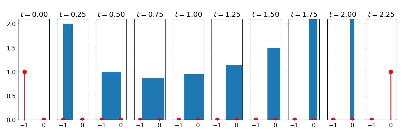
We consider the flow of ℱδ0\mathcal{F}_{\delta_{0}} starting at the initial measure γ⁡(0)=μ0≔δ−1\gamma(0)=\mu_{0}\coloneqq\delta_{-1}. Due to Qδ0≡0Q_{\delta_{0}}\equiv 0, Proposition 1 yields the gradient flow γ⁡(t)≔(Qt)#​λ(0,1)\gamma(t)\coloneqq(Q_{t})_{\#}\lambda_{(0,1)} given by

γ⁡(t)={δ−1,t=0,12​t​λ[−1,−1+2​t],0≤t≤12,12​t​λ[−1,0]+(1−12​t)​δ0,12<t.\gamma(t)=\begin{cases}\delta_{-1},&t=0,\\ \frac{1}{2t}\lambda_{[-1,-1+2t]},&0\leq t\leq\frac{1}{2},\\ \frac{1}{2t}\lambda_{[-1,0]}+\left(1-\frac{1}{2t}\right)\delta_{0},&\frac{1}{2}<t.\\ \end{cases} (33)

For t∈(0,12]t\in(0,\frac{1}{2}], the initial Dirac measure becomes a uniform measure with increasing support, and for t∈(12,1)t\in(\frac{1}{2},1) it is the convex combination of a uniform measure and δ0\delta_{0}. A visualization of the flow is given in Figure 1. □\Box

Refer to caption
Figure 1: Visualization of the Wasserstein gradient flow of ℱδ0\mathcal{F}_{\delta_{0}} from δ−1\delta_{-1} to δ0\delta_{0}. At various times tt, the absolute continuous part is visualized by its density in blue (area equals mass) and the atomic part by the red dotted vertical line (height equals mass). The atomic part at the end point x=0x=0 starts to grow at time t=12t=\tfrac{1}{2}, where the support of the density touches this point for the first time.

6.2 Flow on Restricted Sets

Next, we are interested in the Wasserstein gradient flows on the subsets 𝒮i\mathcal{S}_{i}, i=1,2i=1,2, given by

  1. (i)

    𝒮1≔{δx:x∈ℝ}\mathcal{S}_{1}\coloneqq\{\delta_{x}\mathrel{\mathop{\ordinarycolon}}x\in\mathbb{R}\},

  2. (ii)

    𝒮2≔{μm,σ=12​3​σλ[m−3​σ,m+3​σ]:m∈ℝ,σ∈ℝ≥0}\mathcal{S}_{2}\coloneqq\{\mu_{m,\sigma}=\frac{1}{2\sqrt{3}\sigma}\lambda_{[m-\sqrt{3}\sigma,m+\sqrt{3}\sigma]}\mathrel{\mathop{\ordinarycolon}}m\in\mathbb{R},\sigma\in\mathbb{R}_{\geq 0}\}.

Note that 𝒮2\mathcal{S}_{2} is a special instance of sets of scaled and translated measures μ∈𝒫2​(ℝ)\mu\in\mathcal{P}_{2}(\mathbb{R}) defined by {Ta,b#μ:a∈ℝ≥0,b∈ℝ}\{{T_{a,b}}_{\#}\mu\mathrel{\mathop{\ordinarycolon}}a\in\mathbb{R}_{\geq 0},b\in\mathbb{R}\}, where Ta,b​(x)≔a​x+bT_{a,b}(x)\coloneqq ax+b. As mentioned in [16] the Wasserstein distance between measures μ1,μ2\mu_{1},\mu_{2} from such sets has been already known to Fréchet:

W22​(μ1,μ2)=|m1−m2|2+|σ1−σ2|2,W_{2}^{2}(\mu_{1},\mu_{2})=|m_{1}-m_{2}|^{2}+|\sigma_{1}-\sigma_{2}|^{2},

where mim_{i} and σi\sigma_{i} are the mean value and standard deviation of μi\mu_{i}, i=1,2i=1,2. This provides an isometric embedding of ℝ×ℝ≥0\mathbb{R}\times\mathbb{R}_{\geq 0} into 𝒫2​(ℝ)\mathcal{P}_{2}(\mathbb{R}). The boundary of 𝒮2\mathcal{S}_{2} is the set of Dirac measures 𝒮1\mathcal{S}_{1} and is isometric to ℝ\mathbb{R}. The sets are convex in the sense that for μ,ν∈𝒮i\mu,\nu\in\mathcal{S}_{i} all geodesics γ:[0,1]→𝒫⁡(ℝ)\gamma\mathrel{\mathop{\ordinarycolon}}[0,1]\to\mathcal{P}(\mathbb{R}) with γ⁡(0)=μ\gamma(0)=\mu and γ⁡(1)=ν\gamma(1)=\nu are in 𝒮i\mathcal{S}_{i}, i∈{1,2}i\in\{1,2\}. For i=1,2i=1,2, we consider

ℱi,ν​(μ)≔{ℱνμ∈𝒮i,+∞otherwise.\mathcal{F}_{i,\nu}(\mu)\coloneqq\begin{cases}\mathcal{F}_{\nu}&\mu\in\mathcal{S}_{i},\\ +\infty&\rm{otherwise}.\end{cases} (34)

Due to the convexity of ℱν\mathcal{F}_{\nu} along geodesics and the convexity of the sets 𝒮i\mathcal{S}_{i}, we obtain that the functions ℱi,ν\mathcal{F}_{i,\nu} are convex along geodesics.

Flows of ℱ1,ν\mathcal{F}_{1,\nu}

We use the notation fx≡xf_{x}\equiv x for the constant function on (0,1)(0,1) with value xx. It is straightforward to check that the function F:L2((0,1))→(−∞,∞]{\rm F}\colon L^{2}((0,1))\to(-\infty,\infty] given by

F⁡(f)={F⁡(x),if ​f=fx​ for some ​x∈ℝ,+∞,otherwise,\displaystyle{\rm F}(f)=\begin{cases}F(x),&$if $f=f_{x}$ for some $x\in\mathbb{R},\\ +\infty,&$otherwise,$\end{cases} (35)

with

F⁡(x)≔∫ℝ|x−y|​𝑑ν​(y)−12​∫ℝ×ℝ|y−z|​𝑑ν​(y)​𝑑ν​(z)F(x)\coloneqq\int_{\mathbb{R}}|x-y|\,\mathrm{d}\nu(y)-\frac{1}{2}\int_{\mathbb{R}\times\mathbb{R}}|y-z|\,\mathrm{d}\nu(y)\mathrm{d}\nu(z)

fulfills F⁡(Qμ)=ℱ1,ν​(μ){\rm F}(Q_{\mu})=\mathcal{F}_{1,\nu}(\mu). In the following, we aim to find x:[0,∞)→ℝx\colon[0,\infty)\to\mathbb{R} satisfying

x˙(t)=−∂F(x(t)).\dot{x}(t)=-\partial F(x(t)).

Since the set {Qμ:μ∈𝒮1}\{Q_{\mu}\mathrel{\mathop{\ordinarycolon}}\mu\in\mathcal{S}_{1}\} is a one-dimensional linear subspace of L2​((,,,))L_{2}((0,1)) spanned by the constant one-function f1f_{1}, this yields fx⁡(t)∈−∂F(fx⁡(t))f_{x(t)}\in-\partial{\rm F}(f_{x(t)}) such that the Wasserstein gradient flow is by Theorem 3.2 given by γ⁡(t)=(fx⁡(t))#​λ(0,1)=δx⁡(t)\gamma(t)=(f_{x(t)})_{\#}\lambda_{(0,1)}=\delta_{x(t)}.
In the special case ν=δq\nu=\delta_{q} for some q∈ℝq\in\mathbb{R}, we have

F⁡(x)=|x−q|,∂F⁡(x)={{−1},x<q,[−1,1],x=q,{1},x>q.F(x)=|x-q|,\qquad\partial F(x)=\begin{cases}\{-1\},&x<q,\\ [-1,1],&x=q,\\ \{1\},&x>q.\end{cases}

Therefore, the Wasserstein gradient flow for x⁡(0)=x0≠0x(0)=x_{0}\neq 0 is given by

γ⁡(t)=δx⁡(t),withx⁡(t)={x0+t,x0<q,x0−t,x0>q.,0≤t<|x0−q|\gamma(t)=\delta_{x(t)},\quad\text{with}\quad x(t)=\begin{cases}x_{0}+t,&x_{0}<q,\\ x_{0}-t,&x_{0}>q.\end{cases},\qquad 0\leq t<|x_{0}-q|

and γ⁡(t)=δq\gamma(t)=\delta_{q} for t≥|x0−q|t\geq|x_{0}-q|.

For ν=12​λ[−1,1]\nu=\frac{1}{2}\lambda_{[-1,1]} the gradient flow starting at x0∈[−1,1]x_{0}\in[-1,1] is

x⁡(t)=x0​e−t,t≥0,x(t)=x_{0}e^{-t},\qquad t\geq 0,

and converges to the midpoint of the interval for t→∞t\to\infty. If it starts at x0∈ℝ∖[−1,1]x_{0}\in\mathbb{R}\setminus[-1,1] the gradient flow is

x(t)={x0+t,x0<−1,x0−t,x0>1.,0≤t≤min|x0−1|,|x0+1|,x(t)=\begin{cases}x_{0}+t,&x_{0}<-1,\\ x_{0}-t,&x_{0}>1.\end{cases},\qquad 0\leq t\leq\min{|x_{0}-1|,|x_{0}+1|},

where it reaches the nearest interval end point in finite time. In Figure 2, we plotted the x⁡(t)x(t) for different initial values x⁡(0)x(0).

Refer to caption
Refer to caption
Figure 2: Wasserstein gradient flow of ℱ1,ν\mathcal{F}_{1,\nu} for ν=δ0\nu=\delta_{0} (left) and ν=12​λ[−1,1]\nu=\frac{1}{2}\lambda_{[-1,1]} (right) from various initial points δx\delta_{x}, x∈[−2,2]x\in[-2,2]. The support of the right measure ν\nu is depicted by the blue region. The examples show that gradient flows may reach the optimal points in finite or infinite time.

Flows of ℱ2,ν\mathcal{F}_{2,\nu}

We observe that Qμm,σ=fm,σQ_{\mu_{m,\sigma}}=f_{m,\sigma}, where fm,σ​(x)=m+2​3​σ​(x−12)f_{m,\sigma}(x)=m+2\sqrt{3}\sigma(x-\tfrac{1}{2}). By Lemma 1 we obtain that the function F:L2((0,1))→(−∞,∞]{\rm F}\colon L_{2}((0,1))\to(-\infty,\infty] given by

F⁡(f)={F⁡(m,σ),if ​f=fm,σ​ for ​(m,σ)∈ℝ×ℝ≥0,+∞,otherwise,\displaystyle{\rm F}(f)=\begin{cases}F(m,\sigma),&$if $f=f_{m,\sigma}$ for $(m,\sigma)\in\mathbb{R}\times\mathbb{R}_{\geq 0},\\ +\infty,&$otherwise,$\end{cases} (36)

fulfills F⁡(Qμ)=ℱ2,ν​(μ){\rm F}(Q_{\mu})=\mathcal{F}_{2,\nu}(\mu), where

F⁡(m,σ)≔∫(0,1)(1−2​s)​(fm,σ​(s)+Qν​(s))​𝑑s+∫(0,1)2|fm,σ​(s)−Qν​(t)|​𝑑t​𝑑s,F(m,\sigma)\coloneqq\int_{(0,1)}(1-2s)(f_{m,\sigma}(s)+Q_{\nu}(s))\mathrm{d}s+\int_{(0,1)^{2}}|f_{m,\sigma}(s)-Q_{\nu}(t)|\mathrm{d}t\mathrm{d}s,

The set {fm,σ:m,σ∈ℝ}\{f_{m,\sigma}\mathrel{\mathop{\ordinarycolon}}m,\sigma\in\mathbb{R}\} is a two dimensional linear subspace of L2​((,,,))L_{2}((0,1)) with orthonormal basis {f1,0,f0,1}\{f_{1,0},f_{0,1}\}. We aim to compute m:[0,∞)→ℝm\colon[0,\infty)\to\mathbb{R} and σ:[0,∞)→ℝ≥0\sigma\colon[0,\infty)\to\mathbb{R}_{\geq 0} with

(m˙(t),σ˙(t))=−∂F(m(t),σ(t)),t∈I⊂ℝ,(\dot{m}(t),\dot{\sigma}(t))=-\partial F(m(t),\sigma(t)),\qquad t\in I\subset\mathbb{R}, (37)

because this yields fm⁡(t),σ⁡(t)∈−∂F(fm⁡(t),σ⁡(t))f_{m(t),\sigma(t)}\in-\partial{\rm F}(f_{m(t),\sigma(t)}) such that γ⁡(t)=(fm⁡(t),σ⁡(t))#​λ(0,1)=μm,σ\gamma(t)=(f_{m(t),\sigma(t)})_{\#}\lambda_{(0,1)}=\mu_{m,\sigma} is by Theorem 3.2 the Wasserstein gradient flow.

In the following, we consider the special case ν=δ0=μ0,0\nu=\delta_{0}=\mu_{0,0}. Then, the function FF reduces to

F⁡(m,σ)\displaystyle F(m,\sigma) =∫ℝ(1−2​s)​(m+2​3​σ​(s−12))+|m+2​3​σ​(s−12)|​𝑑s\displaystyle=\int_{\mathbb{R}}(1-2s)(m+2\sqrt{3}\sigma(s-\tfrac{1}{2}))+|m+2\sqrt{3}\sigma(s-\tfrac{1}{2})|\mathrm{d}s (38)
=−σ3+{|m|,if ​|m|≥3​σ,m2+3​σ22​3​σ2if ​|m|<3​σ,\displaystyle=-\frac{\sigma}{\sqrt{3}}+\begin{cases}|m|,&$if $|m|\geq\sqrt{3}\sigma,\\ \frac{m^{2}+3\sigma^{2}}{2\sqrt{3}\sigma^{2}}&$if $|m|<\sqrt{3}\sigma,\end{cases} (39)

and the subdifferential is given by

∂F⁡(m,σ)={sgn⁡(m)×{−13},if ​|m|≥3​σ,{(m3​σ2,−m23​σ3−13)},if ​|m|<3​σ,sgn⁡(m)={{|m|m},if ​m≠0,[−1,1],if ​m=0.\partial F(m,\sigma)=\begin{cases}\mathrm{sgn}(m)\times\{-\tfrac{1}{\sqrt{3}}\},&$if $|m|\geq\sqrt{3}\sigma,\\ \{(\tfrac{m}{\sqrt{3}\sigma^{2}},\tfrac{-m^{2}}{\sqrt{3}\sigma^{3}}-\frac{1}{\sqrt{3}})\},&$if $|m|<\sqrt{3}\sigma,\end{cases}\quad\mathrm{sgn}(m)=\begin{cases}\{\tfrac{|m|}{m}\},&$if $m\neq 0,\\ [-1,1],&$if $m=0.\end{cases}

We observe that FF is differentiable for σ>0\sigma>0. Thus, for any initial intial value (m⁡(0),σ⁡(0))=(m0,σ0)(m(0),\sigma(0))=(m_{0},\sigma_{0}), we can compute the trajectory (m⁡(t),σ⁡(t))(m(t),\sigma(t)) solving (37) using an ODE solver. In Figure 3 (left), we plotted the level sets of the function F⁡(m,σ)F(m,\sigma) as well as the solution trajectory (m⁡(t),σ⁡(t))(m(t),\sigma(t)) for different initial values (m⁡(0),σ⁡(0))(m(0),\sigma(0)). For (m⁡(0),σ⁡(0))=(−1,0)(m(0),\sigma(0))=(-1,0), the resulting flow is illustrated in Figure 3, right.

Refer to caption
Refer to caption
Figure 3: Wasserstein gradient flow ℱ2,δ0\mathcal{F}_{2,\delta_{0}} from (m⁡(0),σ⁡(0))(m(0),\sigma(0)) to δ0\delta_{0} (left) and from δ−1\delta_{-1} to δ0\delta_{0} (right). In contrast Figure 1 it is a uniform measure for all t∈(0,1)t\in(0,1).
Flows for a Smooth Kernel

For smooth, positive definite kernels KK the MMD functional ℱν≔𝒟K2​(⋅,ν)\mathcal{F}_{\nu}\coloneqq\mathcal{D}_{K}^{2}(\cdot,\nu) is in general not convex and leads to a more complex energy landscape than for the negative distance kernel. This may lead to problems for optimization algorithms. To illustrate this observation, we let ν≔λ[−1,1]\nu\coloneqq\lambda_{[-1,1]} and compare the energy landscape of the restricted functional ℱ2,ν\mathcal{F}_{2,\nu} for K⁡(x,y)≔−|x−y|K(x,y)\coloneqq-|x-y| and the kernel

K~​(x,y)≔{(1−12​|x−y|)2​(|x−y|+1),|x−y|≤2,0,else.\tilde{K}(x,y)\coloneqq\begin{cases}(1-\tfrac{1}{2}|x-y|)^{2}(|x-y|+1),&|x-y|\leq 2,\\ 0,&\text{else.}\end{cases} (40)

In contrast to the negative distance kernel KK, the kernel K~\tilde{K} is positive definite (without restrictions on the aia_{i}), cf. [33], and has a Lipschitz continuous gradient. The two energy landscapes of ℱ2,ν\mathcal{F}_{2,\nu} are visualized in Figure 4. The non-convexity of ℱν\mathcal{F}_{\nu} for K~\tilde{K} is readily seen by the presence of a saddle point for ℱ2,ν\mathcal{F}_{2,\nu} at μ=δ0\mu=\delta_{0} (equivalently to (m,σ)=(0,0)(m,\sigma)=(0,0) in the m​σm\sigma-plane). Note that any Wasserstein gradient flow of ℱν\mathcal{F}_{\nu} starting at a Dirac measure δx\delta_{x} converges to this saddle point μ=δ0\mu=\delta_{0}.

Refer to caption
Refer to caption
Figure 4: Visualization of the energy landscapes of ℱ2,λ[−1,1]\mathcal{F}_{2,\lambda_{[-1,1]}} for the convex negative distance kernel (left) and the non-convex, smooth kernel given in (40). The red dot is the global minimizer λ[−1,1]\lambda_{[-1,1]} (left and right) and the blue point (right) is the saddle point δ0\delta_{0}. The black lines depict selected gradient flows.

7 Conclusions

We provided insight into Wasserstein gradient flows of MMD functionals with negative distance kernels and characterized in particular flows ending in a Dirac measure. We have seen that such flows are not simple particle flows, e.g. starting in another Dirac measure the flow becomes immediately uniformly distributed and after a certain time a mixture of a uniform and a Dirac measure. In our future work, we want to extend our considerations to empirical measures and incorporate deep learning techniques as in [2]. Also the treatment of other functionals which incorporate an interaction energy part appears to be interesting. Further, we may combine univariate techniques with multivariate settings using Radon transform like techniques as in [8, 23, 25].

References

  • [1] Abraham, I., Abraham, R., Bergounioux, M., Carlier, G.: Tomographic reconstruction from a few views: A multi-marginal optimal transport approach. Applied Mathematics and Optimization 75(1), 55–73 (2017)
  • [2] Altekrüger, F., Hertrich, J., Steidl, G.: Neural Wasserstein gradient flows for maximum mean discrepancies with Riesz kernels. arXiv:XXX (2023)
  • [3] Ambrosio, L., Gigli, N., Savare, G.: Gradient Flows. Lectures in Mathematics ETH Zürich, Birkhäuser, Basel (2005)
  • [4] Arbel, M., Korba, A., Salim, A., Gretton, A.: Maximum mean discrepancy gradient flow. In: Wallach, H., Larochelle, H., Beygelzimer, A., d Alché-Buc, F., Fox, E., Garnett, R. (eds.) Advances in Neural Information Processing Systems. vol. 32, pp. 1–11. Curran Associates Inc., New York, USA (2019)
  • [5] Beier, F., Beinert, R., Steidl, G.: On a linear Gromov–Wasserstein distance. IEEE Transactions on Image Processing 31, 7292–7305 (2022)
  • [6] Binkowski, M., Sutherland, D.J., Arbel, M., Gretton, A.: Demystifying MMD GANs. In: Proceedings ICLR 2018. OpenReview (2018)
  • [7] Bonaschi, G.A., Carrillo, J.A., Francesco, M.D., Peletier, M.A.: Equivalence of gradient flows and entropy solutions for singular nonlocal interaction equations in 1d. ESAIM Control Optimization and Calculus of Variation 21, 414–441 (2015)
  • [8] Bonet, C., Courty, N., Septier, F., Drumetz, L.: Efficient gradient flows in sliced-Wasserstein space. Transactions on Machine Learning Research (2022)
  • [9] Bonneel, N., Rabin, J., Peyré, G., Pfister, H.: Sliced and Radon Wasserstein barycenters of measures. Journal of Mathematical Imaging and Vision 1(51), 22–45 (2015)
  • [10] Cai, T., Cheng, J., Schmitzer, B., Thorpe, M.: The linearized Hellinger-Kantorovich distance. arXiv:2102.08807 (2021)
  • [11] Carrillo, J.A., Huang, Y.: Explicit equilibrium solutions for the aggregation equation with power-law potentials. Kinetic and Related Models 10(1), 171–192 (2017)
  • [12] Chafaï, D., Saff, E.B., Womersley, R.S.: Threshold condensation to singular support for a Riesz equilibrium problem. arXiv:2206.04956v1 (2022)
  • [13] Dziugaite, G.K., Roy, D.M., Ghahramani, Z.: Training generative neural networks via maximum mean discrepancy optimization. In: Proceedings UAI 2015. UAI (2015)
  • [14] Ehler, M., Gräf, M., Neumayer, S., Steidl, G.: Curve based approximation of measures on manifolds by discrepancy minimization. Foundations of Computational Mathematics 21(6), 1595–1642 (2021)
  • [15] Feydy, J., Séjourné, T., Vialard, F.X., Amari, S., Trouvé, A., Peyré, G.: Interpolating between optimal transport and MMD using Sinkhorn divergences. In: Proc. of Machine Learning Research. vol. 89, pp. 2681–2690. PMLR (2019)
  • [16] Gelbrich, M.: On a formula for the l2 Wasserstein metric between measures on Euclidean and Hilbert spaces. Mathematische Nachrichten 147(1), 185–203 (1990)
  • [17] Gutleb, T.S., Carrillo, J.A., Olver, S.: Computation of power law equilibrium measures on balls of arbitrary dimension. arXiv:2109.00843v1 (2021)
  • [18] Hertrich, J., Gräf, M., Beinert, R., Steidl, G.: Wasserstein steepest descent flows of disrepancies with Riesz kernels. arXiv:2211.01804 v1) (2022)
  • [19] Jordan, R., Kinderlehrer, D., Otto, F.: The variational formulation of the Fokker–Planck equation. SIAM Journal on Mathematical Analysis 29(1), 1–17 (1998)
  • [20] Kolouri, S., Park, S., Rohde, G.: The Radon cumulative distribution transform and its application to image classification. IEEE Transactions on Image Processing 25(2), 920–934 (2016)
  • [21] Landkof, N.: Foundations of Modern Potential Theory. Grundlehren der mathematischen Wissenschaften, Springer, Berlin (1972)
  • [22] Li, C.L., Chang, W.C., Cheng, Y., Yang, Y., Póczos, B.: MMD GAN: Towards deeper understanding of moment matching network. arXiv:1705.08584 (2017)
  • [23] Liutkus, A., Simsekli, U., Majewski, S., Durmus, A., Stöter, F.R.: Sliced-wasserstein flows: Nonparametric generative modeling via optimal transport and diffusions. In: Proc. of Machine Learning Research, vol. 97. PMLR (2019)
  • [24] Neumayer, S., Steidl, G.: From optimal transport to discrepancy. In: Chen, K., Schönlieb, C.B., Tai, X.C., Younes, L. (eds.) Handbook of Mathematical Models and Algorithms in Computer Vision and Imaging: Mathematical Imaging and Vision, pp. 1–36. Springer (2023)
  • [25] Nguyen, K., Ho, N., Pham, T., Bui, H.: Distributional sliced-wasserstein and applications to generative modeling. In: 9th International Conference on Learning Representations. IEEE (2021)
  • [26] Otto, F.: The geometry of dissipative evolution equations: the porous medium equation. Communications in Partial Differential Equations 26, 101–174 (2001)
  • [27] Park, S., Kolouri, S., Kundu, S., Rohde, G.: The cumulative distribution transform and linear pattern classification. Applied and Computational Harmonic Analysis (2017)
  • [28] Pavliotis, G.A.: Stochastic processes and applications: Diffusion Processes, the Fokker-Planck and Langevin Equations. No. 60 in Texts in Applied Mathematics, Springer, New York (2014)
  • [29] Rockafellar, R.T., Royset, J.O.: Random variables, monotone relations, and convex analysis. Mathematical Programming 148, 297–331 (2014)
  • [30] Saff, E., Totik, V.: Logarithmic Potentials with External Fields. Grundlehren der mathematischen Wissenschaften, Springer, Berlin (1997)
  • [31] Santambrogio, F.: Optimal Transport for Applied Mathematicians, Progress in Nonlinear Differential Equations and their Applications, vol. 87. Birkhäuser, Basel (2015)
  • [32] Villani, C.: Topics in Optimal Transportation. No. 58 in Graduate Studies in Mathematics, American Mathematical Society, Providence (2003)
  • [33] Wendland, H.: Scattered Data Approximation. Cambridge University Press (2005)