Study of Mach reflection in inviscid flows
Abstract
In this paper, we study the Mach reflection phenomenon in inviscid flows using a higher order discontinuous Galerkin method and overset grids. We use the shock capturing procedure proposed in [1] using overset grids to capture the discontinuities occurring in the supersonic flow over a wedge accurately. In this procedure, we obtain a coarse grid solution first and using the troubled cell data, we construct an overset grid which is approximately aligned to all the discontinuities. We rerun the solver with the coarse grid solution as the initial condition while using the troubled cell indicator and the limiter only on the overset grid. This allows us to capture the discontinuities accurately. Using this procedure, we have obtained the solution for Mach and flow over a wedge for various wedge angles and determined the detachment criterion and the Von Neumann condition accurately. We have also determined the Mach stem height for various wedge angles for these Mach numbers. We have also demonstrated the hysteresis that occurs in the transition from regular reflection to Mach reflection.
Keywords: Mach reflection, discontinuous Galerkin method, overset grids, hysteresis
1 Introduction
In this paper, we study the transition between regular reflection (RR) and Mach reflection (MR) of steady shock waves in inviscid flows using discontinuous Galerkin method (DGM) along with overset grids. This has been studied quite extensively in literature experimentally [2], numerically [3], and analytically [4]. We use the shock capturing procedure proposed in [1] using overset grids and a higher order method (DGM) to capture the discontinuities occurring in the supersonic flow over a wedge accurately. In this procedure, we obtain a coarse grid solution first and using the solution and the troubled cell data, we construct an overset grid which is approximately aligned to all the discontinuities. We rerun the solver with the coarse grid solution as the initial condition while using the troubled cell indicator and the limiter only on the overset grid. This allows us to capture the discontinuities accurately. We solve the Euler equations in the computational domain shown in Figure 1 using DGM and overset grids for Mach 3.0 and 4.0 flow over a wedge for different wedge angles to determine the transition between RR and MR. In this way, we determine the detachment criterion and the Von Neumann condition accurately to demonstrate the hysteresis that occurs in such a flow.
The paper is organized as follows. We describe the formulation of the discontinuous Galerkin method used for all our results in Section 2, the procedure used for shock capturing using overset grids is described in Section 3, the results are described in Section 4 and we conclude the paper in Section 5.
2 Description of discontinuous Galerkin method
Consider the Euler equations in conservative form as given by
| (1) |
where , and with and . Here, is the density, is the velocity, is the total energy and is the pressure. We approximate the domain by non overlapping elements given by .
We look at solving (1) using the discontinuous Galerkin method. We approximate the local solution in an element , where is the element number, as a polynomial of order which is given by:
| (2) |
where and and are the local coordinates. Here, the subscript represents the particular degree of freedom, represents the grid size, and the superscript is the element number. The polynomial basis used () is the tensor product orthonormalized Legendre polynomials of degree . The number of degrees of freedom are given by . Now, using as the test function, the weak form of the equation (1) is obtained as
| (3) |
where is the boundary of , and where is the monotone numerical flux at the interface which is calculated using an exact or approximate Riemann solver and is the unit outward normal. This is termed to be based discontinuous Galerkin method.
Equation (3) is integrated using an appropriate Gauss Legendre quadrature and is discretized in time by using the fifth order Runge-Kutta time discretization given in [5] unless otherwise specified. To control spurious oscillations which occur near discontinuities, a limiter is used with a troubled cell indicator. We have used the KXRCF troubled cell indicator [6] and the compact subcell WENO (CSWENO) limiter proposed in [7] for all our calculations.
3 Overset grids and shock capturing
Overset grids consist of multiple grids which overlap each other as shown in Figure 2. When using DGM on overset grids, there are two possible approaches to handle data communication between the grids. One is a face based communication approach developed in [8], where solutions at an overset interface are obtained from the donor element, and then the boundary condition is applied weakly by imposing a numerical flux at the flux interpolation points. The other is an element based communication approach developed in [9], where the internal degrees of freedom of cells near the overset interface are obtained from the donor element. We use the new element based communication approach developed in [10] for the data communication between the grids.


For capturing the shocks accurately, we use the procedure developed in [1] using overset grids. A brief explanation of the procedure is given below:
Step 1: Run the solver on a coarse grid with a given troubled cell indicator and limiter to steady state and obtain the solution. As an example, we show the coarse grid solution obtained for Mach 3.0 flow over a wedge in Figure 3
Step 2: Look at the troubled cells to locate the discontinuities (shocks) that occur in the solution. The troubled cell profile obtained for the Mach 3.0 flow over a wedge using the KXRCF troubled cell indicator [6] is shown in Figure 4. From this figure, we can see that the troubled cells give us a good idea of the location of the shocks, the contact discontinuity and the initial expansion that forms near the wedge.
Step 3: Construct an overset grid conforming to the computational domain which is refined in a direction perpendicular to the discontinuities such that they are approximately parallel to a grid line. This overset grid also encompasses all the troubled cells. An example overset grid constructed in such a fashion for the Mach 3.0 flow over a wedge is shown in Figure 5.
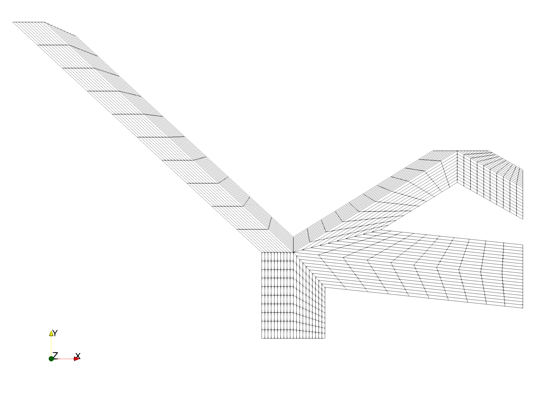
Step 4: Using this overset grid, we rerun the solver with the coarse grid solution as the initial condition. While running the solver, we use the troubled cell indicator and the limiter only on the overset grid. We also use a high resolution numerical flux on the overset grid to capture the shock accurately. We have used the SLAU2 [11] numerical flux in the overset grid and the less expensive Lax-Friedrichs flux elsewhere. Using this procedure, we obtain a more accurate solution with the discontinuities approximately aligned to a grid line. The final solution obtained in this fashion for Mach 3.0 flow over a wedge is shown in Figure 6.

Regarding the computational cost of the scheme proposed for the current problem, we note that the troubled cell data shown in Figure 4 are obtained from a coarse grid of 20000 elements using based DGM after converging to a residue of about which happens in about 8000 iterations. This coarse grid solution is not a fully converged solution but is good enough to be used as an initial condition for the overset grid higher order ( based DGM) solution. The time taken per iteration per degree of freedom using based DGM for this problem is about s. This tells us that the coarse grid troubled cell data is obtained in about s which is a little less than 12 minutes. Most of the work involved is in constructing the overset grid which is done manually. After the overset grid is constructed and the solver is run on the new grid with the coarse grid solution as the initial condition, the residue converges to in about 32000 iterations. For based DGM, the time taken per iteration per degree of freedom is about s for this problem. This tells us that the final solution (which is fifth order accurate) is obtained in about s which is about six hours. All these calculations are done on a 3.60 GHz, Intel(R) Core(TM) i7-7700 CPU with a single thread. The calculations for remaining angles are quite similar. We also note that we have a parallelised code and we obtain the solution much faster based on the number of threads used.
4 Results
1) Mach number 3.0: We solve the two-dimensional Euler equations given by (1) using the discontinuous Galerkin method for various wedge angles between and near the transition criterion (transition from Regular reflection to Mach reflection) for Mach number 3.0 and in the computational domain shown in Figure 1. We consider two cases to demonstrate the hysteresis phenomenon. We solve the equations using an impulsive start as the initial condition for the first case, and the converged solution for as the second case. The first case is a numerical model to obtain the detachment criterion and the second case demonstrates the Von Neumann condition. Using the procedure outlined in Section 3, we obtain a very accurate solution for each of the wedge angles and obtain the transition criterion clearly. Note that the initial conditions mentioned above are used to obtain the coarse grid solution first and the coarse grid solution is used as an initial condition to get the fine grid solution using based DGM. To show that the transition criterion has been captured accurately, we show the solution obtained for Mach 3.0 flow over a wedge with wedge angles and with the case 1 initial conditions in Figures 7 and 8 respectively.


We also show the table containing the Mach stem height obtained using this procedure for various wedge angles for both cases of initial conditions in Table 1. From Table 1, we can see that the transition criterion occurs between wedge angles and and the Von Neumann transition criterion occurs between wedge angles and . From the three-shock theory, the transition criterion is at and the Von Neumann condition occurs at . This closely agrees with what we have obtained and validates our procedure.
| for case 1 | for case 2 | |
| (impulsive start) | (converged solution for ) | |
| 0.274 | - | |
| 0.233 | 0.233 | |
| 0.188 | 0.188 | |
| 0.153 | 0.153 | |
| 0.122 | 0.122 | |
| 0.078 | 0.078 | |
| RR | 0.066 | |
| RR | 0.041 | |
| RR | 0.028 | |
| RR | 0.009 | |
| RR | 0.002 | |
| RR | RR | |
| RR | RR |
2) Mach number 4.0: We repeat the same procedure for various wedge angles between and near the transition criterion (transition from Regular reflection to Mach reflection) for Mach number 4.0 and in the computational domain shown in Figure 1. Again, we consider two cases to demonstrate the hysteresis phenomenon. We solve the equations using an impulsive start as the initial condition for the first case, and the converged solution for as the second case. We show the table containing the Mach stem height obtained using this procedure for various wedge angles for both cases of initial conditions in Table 2. From Table 2, we can see that the transition criterion occurs between wedge angles and and the Von Neumann transition criterion occurs between wedge angles and . From the three-shock theory, the transition criterion for Mach number is at and the Von Neumann condition occurs at . This closely agrees with what we have obtained and validates our procedure.
| for case 1 | for case 2 | |
| (impulsive start) | (converged solution for ) | |
| 0.344 | - | |
| 0.313 | 0.313 | |
| 0.285 | 0.285 | |
| 0.245 | 0.245 | |
| RR | 0.224 | |
| RR | 0.203 | |
| RR | 0.183 | |
| RR | 0.144 | |
| RR | 0.115 | |
| RR | 0.093 | |
| RR | 0.045 | |
| RR | 0.005 | |
| RR | 0.002 | |
| RR | RR | |
| RR | RR |
5 Conclusion
We have demonstrated the transition between regular reflection (RR) and Mach reflection (MR) of steady shock waves in inviscid flows using discontinuous Galerkin method (DGM) along with overset grids using an accurate shock capturing procedure [1]. We have identified the detachment criterion and the Von Neumann condition accurately and demonstrated the hysteresis which occurs in the transition. We have also calculated the Mach stem height for various wedge angles for Mach numbers 3.0 and 4.0. As future work, this shock capturing procedure can be used to further study the different flow phenomena that occur when the inflow Mach number is small ().
References
- [1] Siva Prasad Kochi S.R. and Ramakrishna M., “Shock capturing with discontinuous Galerkin Method using Overset grids for two-dimensional Euler equations,” 2020. Paper under review in J. Comput. Phys. Preprint at https://arxiv.org/abs/2003.01378.
- [2] Chpoun A., Passerel D., Li H. and Ben-Dor G., “Reconsideration of the state-of-the-art of oblique shock wave reflection in steady flows. Part I: Experimental investigation,” J. Fluid. Mech., vol. 301, pp. 19–35, 1995.
- [3] Vuillon J., Zeitoun D. and Ben-Dor G., “Reconsideration of the state-of-the-art of oblique shock wave reflection in steady flows. Part 2: Numerical investigation,” J. Fluid. Mech., vol. 301, pp. 37–50, 1995.
- [4] Ben-Dor G., Shock wave reflection phenomena. New York: Springer, 2007.
- [5] Butcher J.C., Numerical Methods for Ordinary Differential Equations. 3rd edition: John Wiley and Sons, 2016.
- [6] Krivodonova L., Xin J., Remacle J.-F., Chevaugeon N. and Flaherty J., “Shock detection and limiting with discontinuous Galerkin methods for hyperbolic conservation laws,” Appl. Numer. Math., vol. 48, pp. 323–338, 2004.
- [7] Siva Prasad Kochi S.R. and Ramakrishna M., “A compact subcell WENO limiting strategy using immediate neighbours for Runge-Kutta discontinuous Galerkin methods,” Int. J. Comput. Math., vol. 98(3), pp. 608–626, 2021.
- [8] Galbraith M.C., Benek J.A., Orkwis P.D. and Turner M.G., “A Discontinuous Galerkin Chimera scheme,” Computers and Fluids, vol. 98, pp. 27–53, 2014.
- [9] Nastase C.R., Mavriplis D.J. and Sitaraman J., “An Overset Unstructured Mesh Discontinuous Galerkin Approach for Aerodynamic Problems,” AIAA 2011-195, 2011.
- [10] Siva Prasad Kochi S.R. and Ramakrishna M., “A Discontinuous Galerkin Overset Scheme Using WENO Reconstruction and Subcells for Two-Dimensional Problems,” J. Sci. Comput., vol. 93:35, 2022.
- [11] Kitamura K. and Shima E., “Towards shock-stable and accurate hypersonic heating computations: A new pressure flux for AUSM-family schemes,” J. Comput. Phys., vol. 245, pp. 62–83, 2013.