跳到论文正文
W Papers独立论文阅读器 arXiv:2301.04296 论文正文 计算阅读时间 · 0%
引用这篇论文根据当前论文元数据生成,正式投稿前建议核对。


License: arXiv.org perpetual non-exclusive license
arXiv:2301.04296v1 [math.ST] 11 Jan 2023

A degree-corrected Cox model for dynamic networksThe authors are listed in the alphabetical order.

Yuguo Chen Note: Department of Statistics, University of Illinois at Urbana-Champaign, Champaign, IL 61820. Email: yuguo@illinois.edu.    Lianqiang Qu Note: School of Mathematics and Statistics, Central China Normal University, Wuhan, Hubei, 430079, P.R.China. Email: qulianq@ccnu.edu.cn.    Jinfeng Xu Note: Department of Biostatistics, City University of Hong Kong, Tat Chee Avenue, Kowloon, Hong Kong. Email: jinfengxu@gmail.com.    Ting Yan Note: Department of Statistics, Central China Normal University, Wuhan, P.R. China, 430079. Email: tingyanty@mail.ccnu.edu.cn.    Yunpeng Zhou Note: Department of Statistics and Actuarial Science, The University of Hong Kong, Hong Kong. Email: u3514104@connect.hku.hk. Affiliation: 22footnotemark: 2 University of Illinois at Urbana-Champaign, Affiliation: 33footnotemark: 3 55footnotemark: 5 Central China Normal University, Affiliation: 44footnotemark: 4 City University of Hong Kong, Affiliation: 66footnotemark: 6 The University of Hong Kong
Abstract

Continuous time network data have been successfully modeled by multivariate counting processes, in which the intensity function is characterized by covariate information. However, degree heterogeneity has not been incorporated into the model which may lead to large biases for the estimation of homophily effects. In this paper, we propose a degree-corrected Cox network model to simultaneously analyze the dynamic degree heterogeneity and homophily effects for continuous time directed network data. Since each node has individual-specific in- and out-degree effects in the model, the dimension of the time-varying parameter vector grows with the number of nodes, which makes the estimation problem non-standard. We develop a local estimating equations approach to estimate unknown time-varying parameters, and establish consistency and asymptotic normality of the proposed estimators by using the powerful martingale process theories. We further propose test statistics to test for trend and degree heterogeneity in dynamic networks. Simulation studies are provided to assess the finite sample performance of the proposed method and a real data analysis is used to illustrate its practical utility.

Key words: Degree heterogeneity; Dynamic Network; Homophily; Kernel smoothing; Multivariate counting process.

1 Introduction

Networks are very common in a wide variety of fields, including social sciences, biological sciences, transportation systems, and power grids. In networks, nodes are used to represent the entities of interest, and edges are used to represent interactions among the nodes. For instance, in an email network, nodes represent users and edges represent email communications between users. Statistical models are useful tools to analyze the interactions in networks (e.g., Goldenberg et al., 2010; Fienberg, 2012). See Kolaczyk, 2009 for a comprehensive review on the statistical analysis of network data.

In many networks, the interactions (such as emails and phone calls) between nodes vary over time. Modelling and inferring from such dynamic network data has attracted great interests in recent years. One common approach is to aggregate network data on predefined time intervals to obtain a sequence of discrete time-stamped snapshots of random graphs with unweighted or weighted edges. See for example, temporal exponential random graph models (Hanneke et al., 2010; Krivitsky and Handcock, 2014), dynamic stochastic block models (Yang et al., 2011; Matias and Miele, 2017; Pensky, 2019), and dynamic latent space models (Sewell and Chen, 2015a; Sewell and Chen, 2015b). However, observation/interaction times are continuous and irregular in many scenarios, including email networks (Perry and Wolfe, 2013), Twitter direct messages networks (DuBois et al., 2013), and bike share networks (Matias et al., 2018). As discussed in Perry and Wolfe, 2013, inference based on transforming the interaction counts into binary edges depends on the choice of the threshold, which may lead to dramatically different networks and conclusions (De Choudhury et al., 2010). In addition, the aggregation of data also depends crucially on the choice of the time intervals which may lead to different networks and inference as well. Therefore, it is more desirable to develop continuous-time network models to make full use of the data.

One natural way to model continuous time interactions amongst nodes is using counting processes (e.g., Butts, 2008; Vu et al., 2011; DuBois et al., 2013; Matias et al., 2018). For example, Perry and Wolfe, 2013 proposed a Cox-type regression model for intensity function to analyze dynamic directed interactions, and developed partial likelihood inference for their model. Instead of using intensity functions, Sit et al., 2021 proposed to use the rate function to model directed interactions. However, both Perry and Wolfe, 2013 and Sit et al., 2021 assumed that the regression parameters are constant over time. Since the regression parameters often change with time, it is important to know the time-varying effects of covariates on interactions. Recently, Kreiß et al., 2019 extended Perry and Wolfe, 2013’s work to time-varying coefficients Cox model that can characterize temporal effects of covariates on interactions, and established pointwise consistency and asymptotic normality of the local maximum likelihood estimator.

The above literature on counting processes for dynamic networks mainly focus on accounting for the effects of covariates. They do not consider degree heterogeneity, which means individuals exhibit substantial variation in their interactions with others. This is another important feature of many real-world networks. In our simulation studies, we found that the estimator of homophily parameters has a large bias when the degree heterogeneity exists but is not considered in the model; see Figures 2. This phenomenon was also observed by Graham, 2017 in static undirected networks, where the presence of “hub” nodes (i.e., nodes with high degrees), who form many interactions with nodes of different kinds, effectively attenuates measured network homophily. Here homophily means individuals with similar covariate values are easier to form connections with each other.

In this article, we aim to model dynamic degree heterogeneity and homophily effects simultaneously for continuous time directed network data. Our contributions are three-folds. First, we propose a novel model, called degree-corrected Cox network model in (1), to address dynamic degree heterogeneity across the nn nodes in the network. The new model contains a set of 2​n2n time-varying degree parameters measuring dynamic degree heterogeneity and a pp-dimensional time-varying regression coefficient for dynamic homophily effect. A local estimating equations method is developed to estimate 2​n+p2n+p unknown time-varying parameters. Second, we establish consistency and asymptotic normality of the proposed estimators by combining the martingale process theories and kernel smoothing methods. The main challenge is that the dimension of the parameter vector grows with the number of nodes in the network, that is, our setting is in the high-dimensional paradigm. This is different from Perry and Wolfe, 2013 and Kreiß et al., 2019, where the number of unknown parameters of interest is fixed, so their methods cannot be applied here. Third, in practice it is not always clear whether a network has degree heterogeneity, especially when the network is sparse. Thus, we further propose test statistics to check whether there is degree heterogeneity in a dynamic work. To the best of our knowledge, such a test has not yet been explored in existing literature.

The rest of this paper is organized as follows. Section 2 introduces our proposed degree-corrected Cox network model. Section 3 develops a local estimating equations approach to estimate the 2​n+p2n+p parameter functions. Section 4 establishes uniform consistency of the estimators and their point-wise central limit theorems, and constructs confidence intervals for parameters. Section 5 develops testing statistics to test for trend and degree heterogeneity. Section 6 provides simulation studies and presents an application to a real data analysis. All the proofs are presented in the supplementary material.

2 Degree-corrected Cox network model

We consider a network with nn nodes labelled as “1,…,n1,\ldots,n”, and study directed interaction processes amongst nodes. A directed interaction from head node ii to tail node jj means a direct edge from ii to jj. We use [n][n] and [n−1]n[n-1]_{n} to denote the integer sets {1,…,n}\{1,\dots,n\} and {n+1,…,2​n−1},\{n+1,\dots,2n-1\}, respectively. For any two nodes i≠j∈[n]i\neq j\in[n], define Ni​j​(s,t)N_{ij}(s,t) as the number of directed interactions from head node ii to tail node jj in the time interval (s,t].(s,t]. Write Ni​j​(t)=Ni​j​(0,t)N_{ij}(t)=N_{ij}(0,t). Without loss of generality, we assume that the interaction process starts at t=0t=0 with Ni​j​(0)=0N_{ij}(0)=0 for 1≤i≠j≤n.1\leq i\not=j\leq n. The counting process {Ni​j​(t):t≥0}\{N_{ij}(t):t\geq 0\} encodes occurrences of directed interactions from head node ii to tail node jj.

Let Zi​j​(t)Z_{ij}(t) be a pp-dimensional external covariate process for the node pair (i,j).(i,j). The covariate Zi​j​(t)Z_{ij}(t) can be used to measure the similarity or dissimilarity of individual-level characteristics. For example, if individual ii has a dd-dimensional characteristic Xi​(t)X_{i}(t), the pairwise covariate Zi​j​(t)Z_{ij}(t) can be constructed by setting Zi​j​(t)=Xi​(t)⊤​Xj​(t)Z_{ij}(t)=X_{i}(t)^{\top}X_{j}(t), Zi​j​(t)=‖Xi​(t)−Xj​(t)‖2Z_{ij}(t)=\|X_{i}(t)-X_{j}(t)\|_{2}, or Zi​j​(t)=Xi​(t)⊗Xj​(t)Z_{ij}(t)=X_{i}(t)\otimes X_{j}(t). Here ‖x‖2\|x\|_{2} denotes the ℓ2\ell_{2}-norm of any vector x∈ℝdx\in\mathbb{R}^{d} and x⊗yx\otimes y denotes the Kronecker product of the vector xx and the vector yy.

The observations consist of {Ni​j(t),Zi​j(t):i≠j∈[n],t∈[0,τ]},\{N_{ij}(t),Z_{ij}(t):i\neq j\in[n],~t\in[0,\tau]\}, where τ\tau is the termination time of the observation period. Let ℱt\mathcal{F}_{t} denote the σ\sigma-filtration that represents everything that happened up to time tt. Define

λi​j​(t|ℱt)=limΔ​t→0+P⁡(Ni​j​((t+Δ​t)−)−Ni​j​(t−)=1|ℱt)/Δ​t\lambda_{ij}(t|\mathcal{F}_{t})=\lim_{\Delta t\rightarrow 0^{+}}P\big(N_{ij}((t+\Delta t)^{-})-N_{ij}(t^{-})=1|\mathcal{F}_{t}\big)/\Delta t

as the intensity function of Ni​j​(t),N_{ij}(t), where Ni​j​(t−)N_{ij}(t^{-}) denotes the number of interactions before time tt. We propose the following model for the intensity function of Ni​j​(t)N_{ij}(t):

λi​j​(t|ℱt)\displaystyle\lambda_{ij}(t|\mathcal{F}_{t}) =exp⁡{αi​(t)+βj​(t)+Zi​j​(t)⊤​γ​(t)},1≤i≠j≤n,\displaystyle=\exp\{\alpha_{i}(t)+\beta_{j}(t)+Z_{ij}(t)^{\top}\gamma(t)\},\quad 1\leq i\not=j\leq n, (1)

where αi​(t)\alpha_{i}(t) denotes the outgoingness of node ii, βj​(t)\beta_{j}(t) denotes the popularity of node jj, and γ⁡(t)\gamma(t) is a common regression coefficient function. As discussed in Perry and Wolfe, 2013 and Yan et al., 2019, γ⁡(t)\gamma(t) concisely captures and estimates the homophily effects of covariates. The larger the term Zi​j​(t)⊤​γ​(t)Z_{ij}(t)^{\top}\gamma(t) is, the more likely homophilous nodes interact with each other.

Similar to the explanations of model parameters in the p1p_{1} model for static networks (Holland and Leinhardt, 1981), the parameters αi​(t)\alpha_{i}(t) and βj​(t)\beta_{j}(t) measure degree heterogeneity. To see this clearly in our model, we consider the special case that Ni​j​(t)N_{ij}(t) is a Poisson process. Note that the out- and in-degrees for node ii in time interval (s,t](s,t] are ∑k≠iNi​k​(s,t)\sum_{k\neq i}N_{ik}(s,t) and ∑i≠kNi​k​(s,t),\sum_{i\neq k}N_{ik}(s,t), respectively. In the case of the Poisson process, we have

∑k=1,k≠inE⁡{Ni​k​(s,t)}=\displaystyle\sum_{k=1,k\neq i}^{n}E\{N_{ik}(s,t)\}= ∫stexp⁡{αi​(u)}​∑k≠inexp⁡{βk​(u)+Zi​k​(u)⊤​γ​(u)}​𝑑u,\displaystyle\int_{s}^{t}\exp\{\alpha_{i}(u)\}\sum_{k\neq i}^{n}\exp\{\beta_{k}(u)+Z_{ik}(u)^{\top}\gamma(u)\}du, (2)
∑k=1,k≠inE⁡{Nk​i​(s,t)}=\displaystyle\sum_{k=1,k\neq i}^{n}E\{N_{ki}(s,t)\}= ∫stexp⁡{βi​(u)}​∑k≠inexp⁡{αk​(u)+Zk​i​(u)⊤​γ​(u)}​𝑑u.\displaystyle\int_{s}^{t}\exp\{\beta_{i}(u)\}\sum_{k\neq i}^{n}\exp\{\alpha_{k}(u)+Z_{ki}(u)^{\top}\gamma(u)\}du. (3)

As we can see, the larger αi​(t)\alpha_{i}(t) is, the more likely node ii interacts with others. Therefore, αi​(t)​(i∈[n])\alpha_{i}(t)~(i\in[n]) accommodates the out-degree heterogeneity across different nodes. On the other hand, the larger βi​(t)\beta_{i}(t) is, the more likely node ii receives interactions from other nodes, that is, βi​(t)\beta_{i}(t) reflects the in-degree heterogeneity. As a result, the effect of degree heterogeneity can be clearly delineated by estimating the node-specific parameters αi​(t)\alpha_{i}(t) and βj​(t)\beta_{j}(t).

In model (1), if we treat λ0,i​j​(t):=exp⁡{αi​(t)+βj​(t)}\lambda_{0,ij}(t):=\exp\{\alpha_{i}(t)+\beta_{j}(t)\} as the baseline intensity function, it reduces to a network version of the well known Cox regression model. Because of this fact, we call model (1) the degree-corrected Cox network model. Note that if one transforms αi​(t)+βj​(t)\alpha_{i}(t)+\beta_{j}(t) to [αi​(t)+c⁡(t)]+[βj​(t)−c⁡(t)][\alpha_{i}(t)+c(t)]+[\beta_{j}(t)-c(t)] by a unknown function c⁡(t),c(t), then model (1) does not change. For the identifiability of model (1), in what follows we set βn​(t)=0\beta_{n}(t)=0 as in Yan et al., 2016a.

Now, we discuss the differences between our model and those proposed by Perry and Wolfe, 2013, Kreiß et al., 2019 and Kreiß, 2021. In model (1), if we multiply by an indicator function of the receiver set of sender ii and set βj​(t)=0​(j∈[n])\beta_{j}(t)=0~(j\in[n]) and γ⁡(t)=γ\gamma(t)=\gamma, then it reduces to Perry and Wolfe, 2013’s model. There are two major differences between model (1) and Perry and Wolfe, 2013’s model: (1) the regression coefficient γ\gamma is a constant over time in Perry and Wolfe, 2013’s model while it is a unknown function γ⁡(t)\gamma(t) in model (1). Our estimates of γ⁡(t)\gamma(t) can be used for statistical inference on time changes in the effects of covariates; (2) only out-degree heterogeneity is taken into account in Perry and Wolfe, 2013’s model while both out- and in-degree heterogeneity are characterized in our model. The node popularity measured by in-degree parameter βj​(t)\beta_{j}(t) is another important network feature (Sengupta and Chen, 2018). To see how model (1) captures this feature, we compute the log-ratio of ui(1)​(0,t)u_{i}^{(1)}(0,t) to uj(1)​(0,t)u_{j}^{(1)}(0,t), where ui(1)​(0,t)u_{i}^{(1)}(0,t) denotes the first derivative of ui​(0,t)=∑k≠inE⁡{Nk​i​(0,t)}u_{i}(0,t)=\sum_{k\neq i}^{n}E\{N_{ki}(0,t)\} with respect to tt. Then we have

log⁡(ui(1)​(0,t)uj(1)​(0,t))=βi​(t)−βj​(t)+log⁡(∑k≠iexp⁡{αk​(t)+Zk​i​(t)⊤​γ​(t)}∑k≠jexp⁡{αk​(t)+Zk​j​(t)⊤​γ​(t)}).\displaystyle\log\bigg(\frac{u_{i}^{(1)}(0,t)}{u_{j}^{(1)}(0,t)}\bigg)=\beta_{i}(t)-\beta_{j}(t)+\log\bigg(\frac{\sum_{k\neq i}\exp\{\alpha_{k}(t)+Z_{ki}(t)^{\top}\gamma(t)\}}{\sum_{k\neq j}\exp\{\alpha_{k}(t)+Z_{kj}(t)^{\top}\gamma(t)\}}\bigg).

As we can see, node ii tends to be more popular in a network than node jj if βi​(t)>βj​(t)\beta_{i}(t)>\beta_{j}(t) at time tt. Under Perry and Wolfe, 2013’s model, we note that the ratio does not contain the difference βi​(t)−βj​(t)\beta_{i}(t)-\beta_{j}(t). In addition, Perry and Wolfe, 2013 treated the baseline intensity function as a nuisance parameter and focused on estimating γ\gamma.

In model (1), if αi​(t)=α​(t)\alpha_{i}(t)=\alpha(t), i∈[n]i\in[n], and βj​(t)=β​(t)\beta_{j}(t)=\beta(t), j∈[n]j\in[n], then after transforming the baseline function to λ0,i​j​(t)=exp⁡{α⁡(t)+β⁡(t)}\lambda_{0,ij}(t)=\exp\{\alpha(t)+\beta(t)\}, it becomes the model proposed by Kreiß et al., 2019 and Kreiß, 2021. One drawback of the model in Kreiß et al., 2019 and Kreiß, 2021 is that they set the same degree parameters for all nodes which neglects the effect of degree heterogeneity in real-world networks. In model (1), our interest is on estimating not only γ⁡(t)\gamma(t), but also the 2​n2n node-specified parameters αi​(t)\alpha_{i}(t) and βj​(t)\beta_{j}(t). The dimension of parameters increases with the number of nodes in model (1), which is more difficult than the case with fixed dimensional parameters in Kreiß et al., 2019 and Kreiß, 2021. It requires the development of new methods for statistical inference; see Sections 3-5 below.

Finally, our model allows the network to have different edge densities. In particular, it allows the network to be sparse. We call a dynamic network sparse if the ratio of the expected number of edges to n2n^{2} over any time interval (s,t]⊂(0,τ)(s,t]\subset(0,\tau) goes to zero as n→∞.n\rightarrow\infty. Consider the case that supt∈[0,τ][αi​(t)+βj​(t)+Zi​j​(t)⊤​γ​(t)]=−qn,\sup_{t\in[0,\tau]}[\alpha_{i}(t)+\beta_{j}(t)+Z_{ij}(t)^{\top}\gamma(t)]=-q_{n}, where qnq_{n} is a positive constant depending on n.n. Then, by (2) and (3), the expected number of edges over time (s,t](s,t] is

∑i=1n∑j≠i∫stexp⁡{αi​(u)+βj​(u)+Zi​j​(u)⊤​γ​(u)}​𝑑u≤(t−s)​n2​e−qn.\displaystyle\sum_{i=1}^{n}\sum_{j\neq i}\int_{s}^{t}\exp\{\alpha_{i}(u)+\beta_{j}(u)+Z_{ij}(u)^{\top}\gamma(u)\}du\leq(t-s)n^{2}e^{-q_{n}}. (4)

Therefore, qnq_{n} determines the sparsity level of the networks. The larger qnq_{n} is, the sparser the network becomes. If we set qn=c0​log⁡(n)q_{n}=c_{0}\log(n) with a constant c0∈(0,1]c_{0}\in(0,1], then the order of the right hand side of (4) is n2−c0,n^{2-c_{0}}, which is less than n2n^{2}, and the dynamic network is sparse.

3 Local estimating equation approach

Let α⁡(t)=(α1​(t),…,αn​(t))⊤\alpha(t)=(\alpha_{1}(t),\dots,\alpha_{n}(t))^{\top} and β⁡(t)=(β1​(t),…,βn−1​(t))⊤\beta(t)=(\beta_{1}(t),\dots,\beta_{n-1}(t))^{\top}. Define θ⁡(t)=(γ​(t)⊤,α​(t)⊤CLOSE,\theta(t)=(\gamma(t)^{\top},\alpha(t)^{\top}, OPENβ​(t)⊤)⊤\beta(t)^{\top})^{\top}. We use the superscript * to denote the true value (e.g., θ∗​(t)\theta^{*}(t) is the true value of θ⁡(t)\theta(t)). For convenience, define N=n⁡(n−1)N=n(n-1). Let 𝒦h​(u)=h−1​𝒦​(u/h),\mathcal{K}_{h}(u)=h^{-1}\mathcal{K}(u/h), where 𝒦⁡(⋅)\mathcal{K}(\cdot) is a kernel function and hh denotes the bandwidth. Further, we define

ℳi​j​(t,αi​(t),βj​(t),γ⁡(t))=Ni​j​(t)−∫0texp⁡{αi​(s)+βj​(s)+Zi​j​(s)⊤​γ​(s)}​𝑑s.\mathcal{M}_{ij}(t;\alpha_{i}(t),\beta_{j}(t),\gamma(t))=N_{ij}(t)-\int_{0}^{t}\exp\{\alpha_{i}(s)+\beta_{j}(s)+Z_{ij}(s)^{\top}\gamma(s)\}ds.

Under model (1), ℳi​j​(t)=ℳi​j​(t,αi∗​(t),βj∗​(t),γ∗​(t))\mathcal{M}_{ij}(t)=\mathcal{M}_{ij}(t;\alpha_{i}^{*}(t),\beta_{j}^{*}(t),\gamma^{*}(t)) is a zero-mean martingale process (see Lemma 2.3.2 in Fleming and Harrington, 1991). Assume that αi∗​(t),\alpha_{i}^{*}(t), βj∗​(t)\beta_{j}^{*}(t) and γ∗​(t)\gamma^{*}(t) are sufficiently smooth in the sense that as s→ts\to t,

maxi∈[n]⁡|αi∗​(s)−αi∗​(t)|→0,maxj∈[n−1]⁡|βj∗​(s)−βj∗​(t)|→0,maxk∈[p]⁡|γk∗​(s)−γk∗​(t)|→0.\displaystyle\max_{i\in[n]}|\alpha_{i}^{*}(s)-\alpha_{i}^{*}(t)|\to 0,\quad\max_{j\in[n-1]}|\beta_{j}^{*}(s)-\beta_{j}^{*}(t)|\to 0,\quad\max_{k\in[p]}|\gamma_{k}^{*}(s)-\gamma_{k}^{*}(t)|\to 0.

When ss is close to t,t, this leads to

d​ℳi​j​(s)=\displaystyle d\mathcal{M}_{ij}(s)= d​Ni​j​(s)−exp⁡{αi​(s)+βj​(s)+Zi​j​(s)⊤​γ​(s)}​d​s\displaystyle dN_{ij}(s)-\exp\{\alpha_{i}(s)+\beta_{j}(s)+Z_{ij}(s)^{\top}\gamma(s)\}ds
≈\displaystyle\approx d​Ni​j​(s)−exp⁡{αi∗​(t)+βj∗​(t)+Zi​j​(s)⊤​γ∗​(t)}​d​s,\displaystyle dN_{ij}(s)-\exp\{\alpha_{i}^{*}(t)+\beta_{j}^{*}(t)+Z_{ij}(s)^{\top}\gamma^{*}(t)\}ds,

where d​Ni​j​(t)=limΔ​t→0[Ni​j​((t+Δ​t)−)−Ni​j​(t−)].dN_{ij}(t)=\lim_{\Delta t\rightarrow 0}[N_{ij}((t+\Delta t)^{-})-N_{ij}(t^{-})]. For simplicity, let d​ℳi​j​(s,t)=d​Ni​j​(s)−exp⁡{αi∗​(t)+βj∗​(t)+Zi​j​(s)⊤​γ∗​(t)}​d​s.d\mathcal{M}_{ij}(s,t)=dN_{ij}(s)-\exp\{\alpha_{i}^{*}(t)+\beta_{j}^{*}(t)+Z_{ij}(s)^{\top}\gamma^{*}(t)\}ds. Based on these facts, we propose the following local estimating equation

(F​(θ⁡(t))⊤,Q​(θ⁡(t))⊤)⊤=0,\displaystyle(F(\theta(t))^{\top},Q(\theta(t))^{\top})^{\top}=0, (5)

where F⁡(θ⁡(t))=(F1​(θ⁡(t)),…,F2​n−1​(θ⁡(t)))⊤F(\theta(t))=(F_{1}(\theta(t)),\dots,F_{2n-1}(\theta(t)))^{\top} with

Fi​(θ​(t))=\displaystyle F_{i}(\theta(t))= 1n−1​∑j≠i∫0τ𝒦h1​(s−t)​d​ℳi​j​(s,t),i∈[n],\displaystyle\frac{1}{n-1}\sum_{j\neq i}\int_{0}^{\tau}\mathcal{K}_{h_{1}}(s-t)d\mathcal{M}_{ij}(s,t),~~i\in[n],
Fn+j​(θ​(t))=\displaystyle F_{n+j}(\theta(t))= 1n−1​∑i≠j∫0τ𝒦h1​(s−t)​d​ℳi​j​(s,t),j∈[n−1],\displaystyle\frac{1}{n-1}\sum_{i\neq j}\int_{0}^{\tau}\mathcal{K}_{h_{1}}(s-t)d\mathcal{M}_{ij}(s,t),~~j\in[n-1],

and

Q⁡(θ⁡(t))=1N​∑i=1n∑j≠i∫0τZi​j​(s)​𝒦h2​(s−t)​d​ℳi​j​(s,t).Q(\theta(t))=\frac{1}{N}\sum_{i=1}^{n}\sum_{j\neq i}\int_{0}^{\tau}Z_{ij}(s)\mathcal{K}_{h_{2}}(s-t)d\mathcal{M}_{ij}(s,t).

We estimate θ∗​(t)\theta^{*}(t) by the solution to equation (5), denoted by θ^​(t)=(γ^​(t)⊤,α^​(t)⊤,β^​(t)⊤)⊤\widehat{\theta}(t)=(\widehat{\gamma}(t)^{\top},\widehat{\alpha}(t)^{\top},\widehat{\beta}(t)^{\top})^{\top}.

Now, we discuss the algorithm for solving (5). We adopt a combination of the fixed point iterative method and the Newton-Raphson method by alternatively solving F⁡(θ⁡(t))=0F(\theta(t))=0 and Q⁡(θ⁡(t))=0Q(\theta(t))=0. This is implemented in Algorithm 1, where Step 1 is about solving F⁡(θ⁡(t))=0F(\theta(t))=0 with a given γ⁡(t)\gamma(t) via the fixed point iterative method, and Step 2 is about solving Q⁡(θ⁡(t))=0Q(\theta(t))=0 with given α⁡(t)\alpha(t) and β⁡(t)\beta(t) via the Newton-Raphson method. The stopping criterion in Step 3 is

ϵ(k)=maxi∈[n]⁡|αi[k]​(t)−αi[k−1]​(t)|+maxi∈[n−1]|βi[k]​(t)−βi[k−1]​(t)​|+maxj∈[p]|​γj[k]−γj[k−1]|≤10−3,\epsilon^{(k)}=\max_{i\in[n]}|\alpha_{i}^{[k]}(t)-\alpha_{i}^{[k-1]}(t)|+\max_{i\in[n-1]}|\beta_{i}^{[k]}(t)-\beta_{i}^{[k-1]}(t)|+\max_{j\in[p]}|\gamma_{j}^{[k]}-\gamma_{j}^{[k-1]}|\leq 10^{-3}, (6)

which has good performances in simulation studies and real data analyses in Section 6.

Input: k=0,αi[0]​(t)=0,βj[0]​(t)=0,γ(0)​(t)=0k=0,~\alpha_{i}^{[0]}(t)=0,~\beta_{j}^{[0]}(t)=0,~\gamma^{(0)}(t)=0 and ϵ(0)=1\epsilon^{(0)}=1;
while ϵ(k)>10−3\epsilon^{(k)}>10^{-3} do
Set k←k+1k\leftarrow k+1;
    Step 1: Calculate αi[k]​(t)\alpha_{i}^{[k]}(t) and βj[k]​(t)\beta_{j}^{[k]}(t) by
αi[k]​(t)=\displaystyle\alpha_{i}^{[k]}(t)= log⁡{∑j≠i∫0τ𝒦h1​(s−t)​d​Ni​j​(t)∑j≠i∫0τ𝒦h1​(s−t)​exp⁡{βj[k−1]​(t)+Zi​j​(s)⊤​γ[k−1]​(t)}​𝑑s},\displaystyle\log\Bigg\{\frac{\sum_{j\neq i}\int_{0}^{\tau}\mathcal{K}_{h_{1}}(s-t)dN_{ij}(t)}{\sum_{j\neq i}\int_{0}^{\tau}\mathcal{K}_{h_{1}}(s-t)\exp\{\beta_{j}^{[k-1]}(t)+Z_{ij}(s)^{\top}\gamma^{[k-1]}(t)\}ds}\Bigg\},
βj[k]​(t)=\displaystyle\beta_{j}^{[k]}(t)= log⁡{∑i≠j∫0τ𝒦h1​(s−t)​d​Ni​j​(t)∑i≠j∫0τ𝒦h1​(s−t)​exp⁡{αi[k−1]​(t)+Zi​j​(s)⊤​γ[k−1]​(t)}​𝑑s}.\displaystyle\log\Bigg\{\frac{\sum_{i\neq j}\int_{0}^{\tau}\mathcal{K}_{h_{1}}(s-t)dN_{ij}(t)}{\sum_{i\neq j}\int_{0}^{\tau}\mathcal{K}_{h_{1}}(s-t)\exp\{\alpha_{i}^{[k-1]}(t)+Z_{ij}(s)^{\top}\gamma^{[k-1]}(t)\}ds}\Bigg\}.
   Step 2: Update γ[k]​(t)\gamma^{[k]}(t) by the solution to
1N​∑i=1n∑j≠i∫0τZi​j​(s)​𝒦h2​(s−t)​[d​Ni​j​(s)−exp⁡{αi[k−1]​(t)+βj[k−1]​(t)+Zi​j​(s)⊤​γ​(t)}​𝑑s]=0.\frac{1}{N}\sum_{i=1}^{n}\sum_{j\neq i}\int_{0}^{\tau}Z_{ij}(s)\mathcal{K}_{h_{2}}(s-t)\big[dN_{ij}(s)-\exp\big\{\alpha_{i}^{[k-1]}(t)+\beta_{j}^{[k-1]}(t)+Z_{ij}(s)^{\top}\gamma(t)\big\}ds\big]=0.
   Step 3: Calculate ϵ(k)\epsilon^{(k)} according to (6)
Output: α^i​(t)\widehat{\alpha}_{i}(t), β^j​(t)\widehat{\beta}_{j}(t) and γ^​(t).\widehat{\gamma}(t).
Algorithm 1 An algorithm for solving local estimating equations

4 Theoretical properties

In this section, we present consistency and asymptotic normality of the estimator. To obtain consistency for θ^​(t)\widehat{\theta}(t), we adopt a two-stage procedure. Let η⁡(t)=(α​(t)⊤,β​(t)⊤)⊤\eta(t)=(\alpha(t)^{\top},\beta(t)^{\top})^{\top} and η^γ​(t)\widehat{\eta}_{\gamma}(t) be the estimator obtained by solving F⁡(θ⁡(t))=0F(\theta(t))=0 with a given γ⁡(t)\gamma(t). Define Q^c​(γ​(t))\widehat{Q}_{c}(\gamma(t)) as the profiled function of Q⁡(θ⁡(t))Q(\theta(t)) obtained by replacing η⁡(t)\eta(t) with η^γ​(t)\widehat{\eta}_{\gamma}(t). It is clear that Q^c​(γ^​(t))=0\widehat{Q}_{c}(\widehat{\gamma}(t))=0. In the first stage, we establish the existence of η^γ​(t)\widehat{\eta}_{\gamma}(t) and derive its consistency rate uniformly in t∈[a,b]t\in[a,b] (see Lemma 6 in the supplementary material). In the second stage, we derive the upper bound of the error between γ^​(t)\widehat{\gamma}(t) and γ∗​(t)\gamma^{*}(t) by using the profiled function Q^c​(γ​(t))\widehat{Q}_{c}(\gamma(t)).

For convenience, define πi​j​(t)=αi​(t)+βj​(t)+Zi​j​(t)⊤​γ​(t)\pi_{ij}(t)=\alpha_{i}(t)+\beta_{j}(t)+Z_{ij}(t)^{\top}\gamma(t) and πi​j∗​(t)=αi∗​(t)+βj∗​(t)+Zi​j​(t)⊤​γ∗​(t)\pi_{ij}^{*}(t)=\alpha_{i}^{*}(t)+\beta_{j}^{*}(t)+Z_{ij}(t)^{\top}\gamma^{*}(t). Let 𝕍⁡(t,η⁡(t),γ⁡(t))\mathbb{V}(t;\eta(t),\gamma(t)) denote the Hessian matrix of (5) at θ⁡(t)\theta(t), and write

𝕍⁡(t,η⁡(t),γ⁡(t))=(Vη,η​(t,γ​(t)),Vη,γ​(t)Vγ,η​(t),Vγ,γ​(t)).\mathbb{V}(t;\eta(t),\gamma(t))=\begin{pmatrix}V_{\eta,\eta}(t,\gamma(t)),&V_{\eta,\gamma}(t)\\ V_{\gamma,\eta}(t),&V_{\gamma,\gamma}(t)\end{pmatrix}.

Furthermore, define V∗​(t)=−𝔼⁡{Vη∗,η∗​(t,γ∗​(t))}V^{*}(t)=-\mathbb{E}\{V_{\eta^{*},\eta^{*}}(t,\gamma^{*}(t))\} and vi,j∗​(t)v_{i,j}^{*}(t) be the (i,j)(i,j)th element of V∗​(t),V^{*}(t), where

vi,i∗​(t)=\displaystyle v_{i,i}^{*}(t)= (n−1)−1​∑j≠i𝔼⁡{eπi​j∗​(t)},i∈[n],\displaystyle(n-1)^{-1}\sum_{j\neq i}\mathbb{E}\{e^{\pi_{ij}^{*}(t)}\},\quad~i\in[n],
vn+j,n+j∗​(t)=\displaystyle v_{n+j,n+j}^{*}(t)= (n−1)−1​∑i≠j𝔼⁡{eπi​j∗​(t)},j∈[n−1],\displaystyle(n-1)^{-1}\sum_{i\neq j}\mathbb{E}\{e^{\pi_{ij}^{*}(t)}\},\quad~j\in[n-1],
vi,n+j∗​(t)=\displaystyle v_{i,n+j}^{*}(t)= vn+j,i​(t)=(n−1)−1​𝔼​{eπi​j∗​(t)},i∈[n],j∈[n−1],i≠j,\displaystyle v_{n+j,i}(t)=(n-1)^{-1}\mathbb{E}\{e^{\pi_{ij}^{*}(t)}\},~i\in[n],~j\in[n-1],~i\neq j,

and vi,j∗​(t)=vj,i∗​(t)=0v_{i,j}^{*}(t)=v_{j,i}^{*}(t)=0 otherwise. Let v2​n,2​n∗​(t)=∑i=1nvi​i∗​(t)−∑i=1n∑j=1,j≠i2​n−1vi​j∗​(t).v_{2n,2n}^{*}(t)=\sum_{i=1}^{n}v_{ii}^{*}(t)-\sum_{i=1}^{n}\sum_{j=1,j\neq i}^{2n-1}v_{ij}^{*}(t). Then, define S∗​(t)=(si​j∗​(t))∈ℝ(2​n−1)×(2​n−1),S^{*}(t)=(s_{ij}^{*}(t))\in\mathbb{R}^{(2n-1)\times(2n-1)}, where

si​j∗​(t)={δi​jvi,i∗​(t)+1v2​n,2​n∗​(t),i,j∈[n]​or​i,j=[n−1]n,1v2​n,2​n∗​(t),otherwise.\displaystyle s_{ij}^{*}(t)=\begin{cases}\frac{\delta_{ij}}{v_{i,i}^{*}(t)}+\frac{1}{v_{2n,2n}^{*}(t)},&i,j\in[n]~~\text{or}~~i,j=[n-1]_{n},\\ \frac{1}{v_{2n,2n}^{*}(t)},&~~~\text{otherwise}.\end{cases}

In the above equation, δi​j\delta_{ij} is an indicator function, i.e., δi​j=1\delta_{ij}=1 if i=ji=j and δi​j=0\delta_{ij}=0 otherwise. Let ‖a‖∞=max1≤i≤n⁡|ai|\|a\|_{\infty}=\max_{1\leq i\leq n}|a_{i}| denote the ℓ∞\ell_{\infty}-norm for any vector a=(a1,…,an)⊤.a=(a_{1},\dots,a_{n})^{\top}.

Before presenting consistency and asymptotic normality of the estimator, we introduce the following conditions.

Condition 1.

maxi,j⁡‖Zi​j​(t)‖∞≤κn\max_{i,j}\|Z_{ij}(t)\|_{\infty}\leq\kappa_{n} almost surely, where κn\kappa_{n} could diverge with nn.

Condition 2.

The parameter functions αi∗​(t),βj∗​(t)\alpha_{i}^{*}(t),~\beta_{j}^{*}(t) and γ∗​(t)\gamma^{*}(t) are twice continuously differentiable. In addition, each element of γ(l)​(t)​(l=0,1,2)\gamma^{(l)}(t)~(l=0,1,2) is a bounded function and

θ∗​(t)∈ℬ={θ⁡(t):max⁡supt∈[a,b]i,j⁡|αi(l)​(t)+βj(l)​(t)+Zi​j​(t)⊤​γ(l)​(t)|≤qn​(l=0,1,2)},\displaystyle\theta^{*}(t)\in\mathcal{B}=\bigg\{\theta(t):\max_{i,j}\sup_{t\in[a,b]}\big|\alpha_{i}^{(l)}(t)+\beta_{j}^{(l)}(t)+Z_{ij}(t)^{\top}\gamma^{(l)}(t)\big|\leq q_{n}~(l=0,1,2)\bigg\},

where qnq_{n} could diverge with nn.

Condition 3.

HQ​(γ⁡(t))=limn→∞𝔼⁡{Vγ,γ​(t)−Vγ,η∗​(t)​Vη∗,η∗​(t,γ⁡(t))−1​Vη∗,γ​(t)}H_{Q}(\gamma(t))=\lim_{n\rightarrow\infty}\mathbb{E}\{V_{\gamma,\gamma}(t)-V_{\gamma,\eta^{*}}(t)V_{\eta^{*},\eta^{*}}(t,\gamma(t))^{-1}V_{\eta^{*},\gamma}(t)\} is continuous in a neighbourhood of γ∗​(t)\gamma^{*}(t) and

inft∈[a,b]ρmin​{HQ​(γ∗​(t))}>ς>0,\displaystyle\inf_{t\in[a,b]}\rho_{\min}\big\{H_{Q}(\gamma^{*}(t))\big\}>\varsigma>0,

where ρmin​(M)\rho_{\min}(M) denotes the smallest eigenvalue of the matrix M,M, and ς\varsigma is some constant.

Condition 4.

𝒦⁡(x)\mathcal{K}(x) is a symmetric density function with support [−1,1].[-1,1].

Condition 5.

n​h12→∞,nh_{1}^{2}\rightarrow\infty, n​h2→∞,nh_{2}\rightarrow\infty, n​e2​qn​h15→0ne^{2q_{n}}h_{1}^{5}\rightarrow 0 and n​eqn​h25/2→0ne^{q_{n}}h_{2}^{5/2}\rightarrow 0 as n→∞.n\rightarrow\infty. Moreover, h2=O⁡(h12).h_{2}=O(h_{1}^{2}).

Condition 1 assumes that covariates are bounded above by κn\kappa_{n} uniformly. If Zi​j​(t)Z_{ij}(t) is a binary predictive variable, Condition 1 automatically holds. If Zi​j​(t)Z_{ij}(t)’s are generated from normal distributions with variances bounded above by a constant, Condition 1 still holds with κn=O⁡(log⁡n)\kappa_{n}=O(\log n). Condition 2 requires that parameter functions are sufficiently smooth and the sum of parameter functions and the sum of their first and second derivatives are bounded above by qnq_{n}. Condition 3 is the assumption to ensure the identifiability of γ∗​(t)\gamma^{*}(t). Condition 4 is a standard assumption in nonparametric statistics. The kernel function affects the convergence rate of the estimators only by multiplicative constants and thus has little impact on the rate of convergence (e.g., Fan and Gijbels, 1996). In Condition 5, h1h_{1} and h2h_{2} are the bandwidths for estimating (α⁡(t),β⁡(t))(\alpha(t),\beta(t)) and γ⁡(t)\gamma(t) in (5) respectively. The orders of the bandwidths h1h_{1} and h2h_{2} are determined by the sample size nn and the sparsity parameter qn.q_{n}. If qnq_{n} is an absolute constant, the bandwidths can be chosen as h1=o(n−1/5)h_{1}=o(n^{-1/5}) and h2=o(n−2/5).h_{2}=o(n^{-2/5}).

4.1 Consistency and asymptotic normality

We first present consistency of θ^​(t)\widehat{\theta}(t), whose proof is given in the supplementary material.

Theorem 1.

Suppose that Conditions 1-5 hold. If (qn+1)​e19​qn​κn3​log⁡(n​h1)/(n​h1)→0(q_{n}+1)e^{19q_{n}}\kappa_{n}^{3}\sqrt{\log(nh_{1})/(nh_{1})}\rightarrow 0 as n→∞n\rightarrow\infty, then the estimator θ^​(t)=(η^​(t)⊤,γ^​(t)⊤)⊤\widehat{\theta}(t)=(\widehat{\eta}(t)^{\top},\widehat{\gamma}(t)^{\top})^{\top}, the solution to equation (2), exists and satisfies

supt∈[a,b]‖η^​(t)−η∗​(t)‖∞=Op​((qn+1)​e13​qn​κn3​log⁡n​h1n​h1),\displaystyle\sup_{t\in[a,b]}\|\widehat{\eta}(t)-\eta^{*}(t)\|_{\infty}=O_{p}\left((q_{n}+1)e^{13q_{n}}\kappa_{n}^{3}\sqrt{\frac{\log nh_{1}}{nh_{1}}}\right), (7)
supt∈[a,b]‖γ^​(t)−γ∗​(t)‖∞=Op​((qn+1)​e7​qn​κn2​log⁡n​h1n​h1+1n2​h2).\displaystyle\sup_{t\in[a,b]}\|\widehat{\gamma}(t)-\gamma^{*}(t)\|_{\infty}=O_{p}\left((q_{n}+1)e^{7q_{n}}\kappa_{n}^{2}\sqrt{\frac{\log nh_{1}}{nh_{1}}}+\frac{1}{n^{2}h_{2}}\right). (8)
Remark 1.

The condition in Theorem 1 implies that qnq_{n} can be chosen as c​log⁡(n​h1)c\log(nh_{1}) with c∈(0,1/40)c\in(0,1/40). Therefore, the term on the right-hand side of (4) is of order nc~n^{\widetilde{c}} with c~∈(79/40,2)\widetilde{c}\in(79/40,2), whose ratio to n2n^{2} tends to zero. The condition on qnq_{n} in Theorem 1 appears stronger than what is needed to guarantee the right-hand side of (7) and (8) to go to zero. The reason is that it establishes not only the uniform consistency, but also the existence of the solution to (5). The existence of the solution requires a more stringent condition on qnq_{n} while this point is not explicitly reflected in (7) and (8). This phenomenon also exists in other works (e.g., Chatterjee et al., 2011; Yan et al., 2016b).

Remark 2.

Indeed the uniform convergence rate in Theorem 1 has the familiar bias-variance trade-off in the kernel smoothing literature (e.g., Fan and Gijbels, 1996). Specifically, in the proof of Theorem 1, the bias terms for η^​(t)\widehat{\eta}(t) and γ^​(t)\widehat{\gamma}(t) are of order O⁡(eqn​h12)O(e^{q_{n}}h_{1}^{2}) and O⁡(eqn​h22),O(e^{q_{n}}h_{2}^{2}), respectively. This fact suggests that the bandwidths should be carefully selected to balance the bias and variance. When Condition 5 holds, the biases in Theorem 1 are dominated uniformly by Op​((qn+1)​e13​qn​κn3​log⁡(n​h1)/(n​h1))O_{p}\big((q_{n}+1)e^{13q_{n}}\kappa_{n}^{3}\sqrt{\log(nh_{1})/(nh_{1})}\big) and Op​((qn+1)​e7​qn​κn2​log⁡(n​h1)/(n​h1)+1/(n2​h2)).O_{p}\big((q_{n}+1)e^{7q_{n}}\kappa_{n}^{2}\sqrt{\log(nh_{1})/(nh_{1})}+1/(n^{2}h_{2})\big).

Define μ0=∫𝒦2​(u)​𝑑u,\mu_{0}=\int\mathcal{K}^{2}(u)du, and write HQ​(t)=HQ​(γ∗​(t)).H_{Q}(t)=H_{Q}(\gamma^{*}(t)). Next, we present the asymptotic normality of γ^​(t)\widehat{\gamma}(t).

Theorem 2.

Suppose that Conditions 1-5 hold. If (qn+1)3/2​e15​qn​κn2​[log⁡(n​h1)]3/4/(n​h1)1/4→0(q_{n}+1)^{3/2}e^{15q_{n}}\kappa_{n}^{2}[\log(nh_{1})]^{3/4}/(nh_{1})^{1/4}\rightarrow 0, then (Nh2)1/2Ψ(t)−1/2{γ^(t)−γ∗(t)−{HQ(t)}−1b∗(t)}(Nh_{2})^{1/2}\Psi(t)^{-1/2}\{\widehat{\gamma}(t)-\gamma^{*}(t)-\{H_{Q}(t)\}^{-1}b_{*}(t)\} converges in distribution to a pp-dimensional standard normal distribution, where Ψ⁡(t)={HQ​(t)}−1​Σ​(t)​{HQ​(t)}−1\Psi(t)=\{H_{Q}(t)\}^{-1}\Sigma(t)\{H_{Q}(t)\}^{-1}. Here, Σ⁡(t)\Sigma(t) and b∗​(t)b_{*}(t) are

Σ⁡(t)=\displaystyle\Sigma(t)= μ0N​∑i=1n∑j=1,j≠in𝔼⁡[(Zi​j​(t)−Vγ∗​η∗​(t)​S∗​(t)​ιi​j)⊗2​eπi​j∗​(t)],\displaystyle\frac{\mu_{0}}{N}\sum_{i=1}^{n}\sum_{j=1,j\neq i}^{n}\mathbb{E}\bigg[\Big(Z_{ij}(t)-V_{\gamma^{*}\eta^{*}}(t)S^{*}(t)\iota_{ij}\Big)^{\otimes 2}e^{\pi_{ij}^{*}(t)}\bigg],
b∗​(t)=\displaystyle b_{*}(t)= μ02​N​h1​[∑i=1n∑j≠i𝔼⁡(Zi​j​(t)​exp⁡{πi​j∗​(t)})∑j≠i𝔼⁡(exp⁡{πi​j∗​(t)})+∑j=1n∑i≠j𝔼⁡(Zi​j​(t)​exp⁡{πi​j∗​(t)})∑i≠j𝔼⁡(exp⁡{πi​j∗​(t)})],\displaystyle\frac{\mu_{0}}{2Nh_{1}}\bigg[\sum_{i=1}^{n}\frac{\sum_{j\neq i}\mathbb{E}(Z_{ij}(t)\exp\{\pi_{ij}^{*}(t)\})}{\sum_{j\neq i}\mathbb{E}(\exp\{\pi_{ij}^{*}(t)\})}+\sum_{j=1}^{n}\frac{\sum_{i\neq j}\mathbb{E}(Z_{ij}(t)\exp\{\pi_{ij}^{*}(t)\})}{\sum_{i\neq j}\mathbb{E}(\exp\{\pi_{ij}^{*}(t)\})}\bigg],

where a⊗2=a​a⊤a^{\otimes 2}=aa^{\top} for any vector a,a, and ιi​j\iota_{ij} is a (2​n−1)(2n-1)-dimensional vector with the iith and (n+j)(n+j)th elements being one and others being zero.

Remark 3.

The limiting distribution of γ^​(t)\widehat{\gamma}(t) involves a bias term {HQ​(t)}−1​b∗​(t).\{H_{Q}(t)\}^{-1}b_{*}(t). This is referred to as the so-called incidental parameter problem in econometric literature (Neyman and Scott, 1948; Fernández-Val and Weidner, 2016; Dzemski, 2017). This phenomenon also appears in the network literature (Graham, 2017; Yan et al., 2019). The bias is due to the appearance of the estimator η^​(t)\widehat{\eta}(t) in the profiled function Q⁡(θ),Q(\theta), and the dimension of η^​(t)\widehat{\eta}(t) diverges as n→∞.n\rightarrow\infty. If qnq_{n} is an absolute constant, then {HQ​(t)}−1​b∗​(t)=O⁡(1/(n​h1))\{H_{Q}(t)\}^{-1}b_{*}(t)=O(1/(nh_{1})), which is asymptotically negligible as n​h1→∞nh_{1}\rightarrow\infty.

The asymptotic normality of η^​(t)\widehat{\eta}(t) is presented in the following theorem.

Theorem 3.

Under Conditions 1-5, if (qn+1)​κn3​e23​qn​(log⁡n​h1)1/2/(n​h1)1/4→0(q_{n}+1)\kappa_{n}^{3}e^{23q_{n}}(\log nh_{1})^{1/2}/(nh_{1})^{1/4}\rightarrow 0 as n→∞n\rightarrow\infty, then for any fixed positive integer kk, (nh1)1/2{(μ0S∗(t))−1/2[η^(t)−η∗(t)]}1:k(nh_{1})^{1/2}\big\{(\mu_{0}S^{*}(t))^{-1/2}[\widehat{\eta}(t)-\eta^{*}(t)]\big\}_{1:k} converges in distribution to a kk-dimensional standard normal distribution.

Remark 4.

By Theorem 3, the covariance matrix of (nh1)1/2[η^(t)−η∗(t)]1:k(nh_{1})^{1/2}[\widehat{\eta}(t)-\eta^{*}(t)]_{1:k} is given by the upper left k×kk\times k block of μ0​S∗​(t).\mu_{0}S^{*}(t). In addition, for any fixed i,i, as n​h1→∞nh_{1}\rightarrow\infty, the convergence rate of η^i​(t)\widehat{\eta}_{i}(t) is O((nh1)−1/2eqn/2).O((nh_{1})^{-1/2}e^{q_{n}/2}).

4.2 Confidence intervals for η∗​(t)\eta^{*}(t)

We next construct the pointwise confidence interval for η∗​(t)\eta^{*}(t). Since the asymptotic covariance matrix for η∗​(t)\eta^{*}(t) involves unknown S∗​(t)S^{*}(t) for approximating [V∗​(t)]−1[V^{*}(t)]^{-1}, we use S^​(t)=(s^i​j​(t))i,j∈[2​n−1]\widehat{S}(t)=(\widehat{s}_{ij}(t))_{i,j\in[2n-1]} to estimate it, where the unknown parameters η∗​(t)\eta^{*}(t) and γ∗​(t)\gamma^{*}(t) are replaced by their respective estimators η^​(t)\widehat{\eta}(t) and γ^​(t)\widehat{\gamma}(t), i.e.,

s^i​j​(t)={δi​jv^i,i​(t)+1v^2​n,2​n​(t),i,j∈[n],or​i,j∈[n−1]n,−1v^2​n,2​n​(t),otherwise.\widehat{s}_{ij}(t)=\begin{cases}\frac{\delta_{ij}}{\widehat{v}_{i,i}(t)}+\frac{1}{\widehat{v}_{2n,2n}(t)},&i,j\in[n],\text{or}~~i,j\in[n-1]_{n},\\ -\frac{1}{\widehat{v}_{2n,2n}(t)},&~~~\text{otherwise}.\end{cases}

In the above equation, v^2​n,2​n=∑i=1nv^i​i​(t)−∑i=1n∑j=1,j≠i2​n−1v^i​j​(t)\widehat{v}_{2n,2n}=\sum_{i=1}^{n}\widehat{v}_{ii}(t)-\sum_{i=1}^{n}\sum_{j=1,j\neq i}^{2n-1}\widehat{v}_{ij}(t).

By Theorem 3, the distribution of (n​h1)1/2​{η^​(t)−η∗​(t)}(nh_{1})^{1/2}\big\{\widehat{\eta}(t)-\eta^{*}(t)\big\} is asymptotically equivalent to

S∗​(t)​(h1n)1/2​∫0τ𝒦h1​(s−t)​𝑑ℳ~​(s),S^{*}(t)\left(\frac{h_{1}}{n}\right)^{1/2}\int_{0}^{\tau}\mathcal{K}_{h_{1}}(s-t)d\widetilde{\mathcal{M}}(s),

where ℳ~​(t)=(M~1​(s),…,M~2​n−1​(t))⊤\widetilde{\mathcal{M}}(t)=(\widetilde{M}_{1}(s),\dots,\widetilde{M}_{2n-1}(t))^{\top} with

M~i​(t)=∑k≠iℳi​k​(t)​(i∈[n])​and​M~n+i​(t)=∑k≠iℳk​i​(t)​(i∈[n−1]).\displaystyle\widetilde{M}_{i}(t)=\sum_{k\neq i}\mathcal{M}_{ik}(t)~(i\in[n])~~\text{and}~~\widetilde{M}_{n+i}(t)=\sum_{k\neq i}\mathcal{M}_{ki}(t)~(i\in[n-1]).

Note that M~i​(t)\widetilde{M}_{i}(t) is the sum of local square-integerable martingales. Therefore, by the martingale properties, we can estimate the covariance Ω⁡(t)\Omega(t) of h1/n​∫0τ𝒦h1​(s−t)​𝑑ℳ~​(s)\sqrt{h_{1}/n}\int_{0}^{\tau}\mathcal{K}_{h_{1}}(s-t)d\widetilde{\mathcal{M}}(s) by Ω^(t)=(ω^i​j(t):i,j∈[2n−1])\widehat{\Omega}(t)=(\widehat{\omega}_{ij}(t):i,j\in[2n-1]) with

ω^i​i​(t)=\displaystyle\widehat{\omega}_{ii}(t)= h1n​∑j≠i∫0τ𝒦h12​(s−t)​d​Ni​j​(s),i∈[n],\displaystyle\frac{h_{1}}{n}\sum_{j\neq i}\int_{0}^{\tau}\mathcal{K}_{h_{1}}^{2}(s-t)dN_{ij}(s),~i\in[n],
ω^n+j,n+j​(t)=\displaystyle\widehat{\omega}_{n+j,n+j}(t)= h1n​∑i≠j∫0τ𝒦h12​(s−t)​d​Ni​j​(s),j∈[n−1],\displaystyle\frac{h_{1}}{n}\sum_{i\neq j}\int_{0}^{\tau}\mathcal{K}_{h_{1}}^{2}(s-t)dN_{ij}(s),~j\in[n-1],
ω^i,n+j​(t)=ω^n+j,i​(t)=\displaystyle\widehat{\omega}_{i,n+j}(t)=\widehat{\omega}_{n+j,i}(t)= h1n​∫0τ𝒦h12​(s−t)​d​Ni​j​(s),i∈[n],j∈[n−1],\displaystyle\frac{h_{1}}{n}\int_{0}^{\tau}\mathcal{K}_{h_{1}}^{2}(s-t)dN_{ij}(s),\qquad i\in[n],~j\in[n-1],
ω^i​j​(t)=ω^j​i​(t)=\displaystyle\widehat{\omega}_{ij}(t)=\widehat{\omega}_{ji}(t)= 0,otherwise.\displaystyle 0,\quad\quad\text{otherwise}.

Thus, we estimate the variance of n​h1​{η^i​(t)−ηi∗​(t)}\sqrt{nh_{1}}\{\widehat{\eta}_{i}(t)-\eta_{i}^{*}(t)\} by the iith diagonal element σ^i​i​(t)\widehat{\sigma}_{ii}(t) of S^​(t)​Ω^​(t)​S^​(t)\widehat{S}(t)\widehat{\Omega}(t)\widehat{S}(t).

By arguments similar to Lemma 7 in the supplementary material, we can show

‖S^​(t)​Ω^​(t)​S^​(t)−μ0​S∗​(t)‖max=op​(1),\displaystyle\|\widehat{S}(t)\widehat{\Omega}(t)\widehat{S}(t)-\mu_{0}S^{*}(t)\|_{\max}=o_{p}(1),

where ‖M‖max=maxi,j⁡|mi,j|\|M\|_{\max}=\max_{i,j}|m_{i,j}| denotes the maximum absolute entry-wise norm for any matrix M=(ai,j).M=(a_{i,j}). Let zαz_{\alpha} be the 100​(1−α)100(1-\alpha)th percentile of the standard normal distribution. Then the (1−α)(1-\alpha)-confidence interval for ηi∗​(t)\eta_{i}^{*}(t) is given by

η^i(t)±(nh1)−1/2zα/2σ^i​i1/2(t),i∈[2n−1].\displaystyle\widehat{\eta}_{i}(t)\pm(nh_{1})^{-1/2}z_{\alpha/2}\widehat{\sigma}_{ii}^{1/2}(t),~~i\in[2n-1].
Remark 5.

Since the dimension of η∗​(t)\eta^{*}(t) diverges with the sample size n,n, directly using μ0​S^​(t)\mu_{0}\widehat{S}(t) to estimate μ0​S∗​(t)\mu_{0}S^{*}(t) may result in a large bias for local smoothing estimators with finite sample. Therefore, instead of μ0​S^​(t),\mu_{0}\widehat{S}(t), we consider a sandwich-type estimator S^​(t)​Ω^​(t)​S^​(t)\widehat{S}(t)\widehat{\Omega}(t)\widehat{S}(t) for the variance of n​h1​{η^i​(t)−ηi∗​(t)}.\sqrt{nh_{1}}\{\widehat{\eta}_{i}(t)-\eta_{i}^{*}(t)\}. This is different from the covariance estimator developed by Yan et al., 2019 for static networks, where the maximum likelihood estimator was used.

4.3 Confidence intervals for γ∗​(t)\gamma^{*}(t)

Based on Theorem 2, γ^​(t)\widehat{\gamma}(t) has a non-negligible bias term HQ​(t)−1​b∗​(t).H_{Q}(t)^{-1}b_{*}(t). Therefore, bias-correction is necessary. For this, define

b^​(t)=\displaystyle\widehat{b}(t)= h12​N​[∑i=1n∑j≠iZi​j​(t)​∫0τ𝒦h12​(s−t)​d​Ni​j​(s)∑j≠iexp⁡{π^i​j​(t)}+∑j=1n∑i≠jZi​j​(t)​∫0τ𝒦h12​(s−t)​d​Ni​j​(s)∑i≠jexp⁡{π^i​j​(t)}],\displaystyle\frac{h_{1}}{2N}\bigg[\sum_{i=1}^{n}\frac{\sum_{j\neq i}Z_{ij}(t)\int_{0}^{\tau}\mathcal{K}_{h_{1}}^{2}(s-t)dN_{ij}(s)}{\sum_{j\neq i}\exp\{\widehat{\pi}_{ij}(t)\}}+\sum_{j=1}^{n}\frac{\sum_{i\neq j}Z_{ij}(t)\int_{0}^{\tau}\mathcal{K}_{h_{1}}^{2}(s-t)dN_{ij}(s)}{\sum_{i\neq j}\exp\{\widehat{\pi}_{ij}(t)\}}\bigg],
H^Q​(t)=\displaystyle\widehat{H}_{Q}(t)= 1N​∑i=1n∑j≠iZi​j​(t)⊗2​eπ^i​j​(t)−V^γ^,η^​(t)​S^​(t)​V^η^,γ^​(t),\displaystyle\frac{1}{N}\sum_{i=1}^{n}\sum_{j\neq i}Z_{ij}(t)^{\otimes 2}e^{\widehat{\pi}_{ij}(t)}-\widehat{V}_{\widehat{\gamma},\widehat{\eta}}(t)\widehat{S}(t)\widehat{V}_{\widehat{\eta},\widehat{\gamma}}(t),

where V^γ^,η^​(t)=N−1​(u^1​(t),…,u^2​n−1​(t))\widehat{V}_{\widehat{\gamma},\widehat{\eta}}(t)=N^{-1}(\widehat{u}_{1}(t),\dots,\widehat{u}_{2n-1}(t)) and V^η^,γ^​(t)=n​V^γ^,η^​(t)⊤\widehat{V}_{\widehat{\eta},\widehat{\gamma}}(t)=n\widehat{V}_{\widehat{\gamma},\widehat{\eta}}(t)^{\top} with

u^i​(t)=∑j≠iZi​j​(t)​eπ^i​j​(t),i∈[n]​and​u^n+j​(t)=∑i≠jZi​j​(t)​eπ^i​j​(t),j∈[n−1].\widehat{u}_{i}(t)=\sum_{j\neq i}Z_{ij}(t)e^{\widehat{\pi}_{ij}(t)},~i\in[n]~~\text{and}~~\widehat{u}_{n+j}(t)=\sum_{i\neq j}Z_{ij}(t)e^{\widehat{\pi}_{ij}(t)},~j\in[n-1].

In addition, by the martingale properties, Σ⁡(t)\Sigma(t) can be estimated by

Σ^​(t)=\displaystyle\widehat{\Sigma}(t)= h2N​∑i=1n∑j≠i(Zi​j​(t)−V^γ^,η^​(t)​S^​(t)​ιi​j)⊗2​∫0τ𝒦h22​(u−t)​d​Ni​j​(u).\displaystyle\frac{h_{2}}{N}\sum_{i=1}^{n}\sum_{j\neq i}\Big(Z_{ij}(t)-\widehat{V}_{\widehat{\gamma},\widehat{\eta}}(t)\widehat{S}(t)\iota_{ij}\Big)^{\otimes 2}\int_{0}^{\tau}\mathcal{K}_{h_{2}}^{2}(u-t)dN_{ij}(u).

Finally, we estimate the bias {HQ​(t)}−1​b∗​(t)\{H_{Q}(t)\}^{-1}b_{*}(t) by {H^Q​(t)}−1​b^​(t)\{\widehat{H}_{Q}(t)\}^{-1}\widehat{b}(t) and the covariance Ψ⁡(t)\Psi(t) by Ψ^​(t)={H^Q​(t)}−1​Σ^​(t)​{H^Q​(t)}−1\widehat{\Psi}(t)=\{\widehat{H}_{Q}(t)\}^{-1}\widehat{\Sigma}(t)\{\widehat{H}_{Q}(t)\}^{-1}.

By arguments similar to Lemma 7 in the supplementary material, the absolute entry-wise error tends to zero with probability, that is,

‖{H^Q​(t)}−1​b^​(t)−{HQ​(t)}−1​b∗​(t)‖∞=op​(1)​and​‖Ψ^​(t)−Ψ⁡(t)‖max=op​(1).\displaystyle\|\{\widehat{H}_{Q}(t)\}^{-1}\widehat{b}(t)-\{H_{Q}(t)\}^{-1}b_{*}(t)\|_{\infty}=o_{p}(1)~~~\text{and}~~~\|\widehat{\Psi}(t)-\Psi(t)\|_{\max}=o_{p}(1).

Let b~j​(t)\widetilde{b}_{j}(t) be the jjth element of {H^Q​(t)}−1​b^​(t)\{\widehat{H}_{Q}(t)\}^{-1}\widehat{b}(t), and ψ^j​j​(t)\widehat{\psi}_{jj}(t) be the jjth diagonal element of Ψ^​(t).\widehat{\Psi}(t). Then the (1−α)(1-\alpha)-confidence interval for γj∗​(t)\gamma_{j}^{*}(t) is given by

γ^j(t)−b~j(t)±(Nh2)−1/2zα/2ψ^j​j1/2(t),j∈[p].\widehat{\gamma}_{j}(t)-\widetilde{b}_{j}(t)\pm(Nh_{2})^{-1/2}z_{\alpha/2}\widehat{\psi}_{jj}^{1/2}(t),~~j\in[p].

5 Hypothesis testing

5.1 Tests for Trend

Perry and Wolfe, 2013 and Sit et al., 2021 assumed that γ∗​(t)\gamma^{*}(t) is constant over time, while Kreiß et al., 2019, Kreiß, 2021 and our proposed model (1) assume that γ∗​(t)\gamma^{*}(t) is time-varying. Whether the effects of covariates on interactions change with time is usually unknown. If both η∗​(t)\eta^{*}(t) and γ∗​(t)\gamma^{*}(t) are time-invariant, the network may be static. Therefore, it is of interest to test if η∗​(t)\eta^{*}(t) and γ∗​(t)\gamma^{*}(t) have time-varying trends. We call this the trend testing problem. In this section, we consider testing the following hypotheses:

H0​η:η∗​(t)=η∗​for all​t∈[a,b]\displaystyle H_{0\eta}:\eta^{*}(t)=\eta^{*}~~\text{for~all}~~t\in[a,b]
versus H1​η:η∗​(t)≠η∗​for some​t∈[a,b],\displaystyle H_{1\eta}:\eta^{*}(t)\neq\eta^{*}~~\text{for some}\ t\in[a,b],

and

H0​γ:γ∗​(t)=γ∗​for all​t∈[a,b]\displaystyle H_{0\gamma}:\gamma^{*}(t)=\gamma^{*}~~\text{for~all}~~t\in[a,b]
versus H1​γ:γ∗​(t)≠γ∗​for some​t∈[a,b],\displaystyle H_{1\gamma}:\gamma^{*}(t)\neq\gamma^{*}~~\text{for some}\ t\in[a,b],

where η∗\eta^{*} and γ∗\gamma^{*} are some unspecified vectors. We see that

  • •

    if either of H0​ηH_{0\eta} and H0​γH_{0\gamma} holds, then model (1) is a semi-parametric model;

  • •

    if both H0​ηH_{0\eta} and H0​γH_{0\gamma} hold, then model (1) becomes a completely parametric model.

Kreiß, 2021 proposed a test statistic which compares the completely parametric and the non-parametric estimator using the ℓ2\ell_{2}-distance to test H0​ηH_{0\eta} and H0​γ.H_{0\gamma}. However, since the dimension of parameters grows with the nodes under model (1), the method developed for fixed dimension in Kreiß, 2021 can not be directly applied here. We consider the following test statistics to test H0​ηH_{0\eta} and H0​γ,H_{0\gamma}, respectively:

𝒯η\displaystyle\mathcal{T}_{\eta} =max⁡supa≤t1<t2≤bi∈[2​n−1]⁡n​h1​|η^i​(t1)−η^i​(t2)|/ϑ^i,η1/2​(t1,t2),\displaystyle=\max_{i\in[2n-1]}\sup_{a\leq t_{1}<t_{2}\leq b}\sqrt{nh_{1}}\big|\widehat{\eta}_{i}(t_{1})-\widehat{\eta}_{i}(t_{2})\big|/\widehat{\vartheta}_{i,\eta}^{1/2}(t_{1},t_{2}),
𝒯γ\displaystyle\mathcal{T}_{\gamma} =max⁡supa≤t1<t2≤bj∈[p]⁡N​h2​|γ^j​(t1)−b~j​(t1)−γ^j​(t2)+b~j​(t2)|/ϑ^j,γ1/2​(t1,t2),\displaystyle=\max_{j\in[p]}\sup_{a\leq t_{1}<t_{2}\leq b}\sqrt{Nh_{2}}\big|\widehat{\gamma}_{j}(t_{1})-\widetilde{b}_{j}(t_{1})-\widehat{\gamma}_{j}(t_{2})+\widetilde{b}_{j}(t_{2})\big|/\widehat{\vartheta}_{j,\gamma}^{1/2}(t_{1},t_{2}),

where ϑ^i,η​(t1,t2)=σ^i​i​(t1)+σ^i​i​(t2)\widehat{\vartheta}_{i,\eta}(t_{1},t_{2})=\widehat{\sigma}_{ii}(t_{1})+\widehat{\sigma}_{ii}(t_{2}) and ϑ^j,γ​(t1,t2)=ψ^j​j​(t1)+ψ^j​j​(t2).\widehat{\vartheta}_{j,\gamma}(t_{1},t_{2})=\widehat{\psi}_{jj}(t_{1})+\widehat{\psi}_{jj}(t_{2}).

The test statistics 𝒯η\mathcal{T}_{\eta} and 𝒯γ\mathcal{T}_{\gamma} are close to zero under the nulls H0​ηH_{0\eta} and H0​γ,H_{0\gamma}, respectively. Hence we will reject H0​ηH_{0\eta} if 𝒯η>cη​(ν),\mathcal{T}_{\eta}>c_{\eta}(\nu), and reject H0​γH_{0\gamma} if 𝒯γ>cγ​(ν),\mathcal{T}_{\gamma}>c_{\gamma}(\nu), where cη​(ν)c_{\eta}(\nu) and cγ​(ν)c_{\gamma}(\nu) are the critical values. To obtain these critical values, we consider a resampling approach. Using arguments similar to the proof of Theorem 3, we can show that under the null H0​η,H_{0\eta}, the distribution of n​h1​[η^​(t1)−η^​(t2)]\sqrt{nh_{1}}[\widehat{\eta}(t_{1})-\widehat{\eta}(t_{2})] is asymptotically equivalent to

h1n​[S^​(t1)​∫0τ𝒦h1​(u−t1)​𝑑ℳ~​(u)−S^​(t2)​∫0τ𝒦h1​(u−t2)​𝑑ℳ~​(u)],\displaystyle\sqrt{\frac{h_{1}}{n}}\bigg[\widehat{S}(t_{1})\int_{0}^{\tau}\mathcal{K}_{h_{1}}(u-t_{1})d\widetilde{\mathcal{M}}(u)-\widehat{S}(t_{2})\int_{0}^{\tau}\mathcal{K}_{h_{1}}(u-t_{2})d\widetilde{\mathcal{M}}(u)\bigg],

and n​h1​[η^​(t1)−η∗]\sqrt{nh_{1}}[\widehat{\eta}(t_{1})-\eta^{*}] and n​h1​[η^​(t2)−η∗]\sqrt{nh_{1}}[\widehat{\eta}(t_{2})-\eta^{*}] are asymptotically independent with t1≠t2.t_{1}\neq t_{2}. In addition, using arguments similar to the proof of Theorem 2, we have that under the null H0​γ,H_{0\gamma}, the distribution of N​h2​[γ^​(t1)−b^​(t1)−γ^​(t2)+b^​(t2)]\sqrt{Nh_{2}}[\widehat{\gamma}(t_{1})-\widehat{b}(t_{1})-\widehat{\gamma}(t_{2})+\widehat{b}(t_{2})] is asymptotically equivalent to

h2N∑i=1n∑j≠i[(Zi​j(t1)−V^γ^,η^(t1)S^(t1)ιi​s)∫0τ𝒦h2(u−t1)dℳi​j(u)\displaystyle\sqrt{\frac{h_{2}}{N}}\sum_{i=1}^{n}\sum_{j\neq i}\bigg[\Big(Z_{ij}(t_{1})-\widehat{V}_{\widehat{\gamma},\widehat{\eta}}(t_{1})\widehat{S}(t_{1})\iota_{is}\Big)\int_{0}^{\tau}\mathcal{K}_{h_{2}}(u-t_{1})d\mathcal{M}_{ij}(u)
−(Zi​j(t2)−V^γ^,η^(t2)S^(t2)ιi​j)∫0τ𝒦h2(u−t2)dℳi​j(u)],\displaystyle\hskip 86.72377pt-\Big(Z_{ij}(t_{2})-\widehat{V}_{\widehat{\gamma},\widehat{\eta}}(t_{2})\widehat{S}(t_{2})\iota_{ij}\Big)\int_{0}^{\tau}\mathcal{K}_{h_{2}}(u-t_{2})d\mathcal{M}_{ij}(u)\bigg],

and N​h2​[γ^​(t1)−b^​(t1)−γ∗]\sqrt{Nh_{2}}[\widehat{\gamma}(t_{1})-\widehat{b}(t_{1})-\gamma^{*}] and N​h2​[γ^​(t2)−b^​(t2)−γ∗]\sqrt{Nh_{2}}[\widehat{\gamma}(t_{2})-\widehat{b}(t_{2})-\gamma^{*}] are asymptotically independent with t1≠t2.t_{1}\neq t_{2}. A direct calculation yields that the variance function of ℳi​j​(u)\mathcal{M}_{ij}(u) is E​{Ni​j​(u)}E\{N_{ij}(u)\} (see Theorem 2.5.3 in Fleming and Harrington, 1991). Motivated by the work of Lin et al., 1994, we replace ℳi​j​(u)\mathcal{M}_{ij}(u) with Ni​j​(u)​Gi​j,N_{ij}(u)G_{ij}, that is,

T~η​(t1,t2)=\displaystyle\widetilde{T}_{\eta}(t_{1},t_{2})= h1n​[S^​(t1)​∫0τ𝒦h1​(u−t1)​𝑑𝒩~​(u)−S^​(t2)​∫0τ𝒦h1​(u−t2)​𝑑𝒩~​(u)],\displaystyle\sqrt{\frac{h_{1}}{n}}\bigg[\widehat{S}(t_{1})\int_{0}^{\tau}\mathcal{K}_{h_{1}}(u-t_{1})d\widetilde{\mathcal{N}}(u)-\widehat{S}(t_{2})\int_{0}^{\tau}\mathcal{K}_{h_{1}}(u-t_{2})d\widetilde{\mathcal{N}}(u)\bigg],
T~γ​(t1,t2)=\displaystyle\widetilde{T}_{\gamma}(t_{1},t_{2})= h2N∑i=1n∑j≠i[H^Q−1(t1)(Zi​j(t1)−V^γ^,η^(t1)S^(t1)ιi​j)∫0τ𝒦h2(u−t1)dNi​j(u)Gi​j\displaystyle\sqrt{\frac{h_{2}}{N}}\sum_{i=1}^{n}\sum_{j\neq i}\bigg[\widehat{H}_{Q}^{-1}(t_{1})\Big(Z_{ij}(t_{1})-\widehat{V}_{\widehat{\gamma},\widehat{\eta}}(t_{1})\widehat{S}(t_{1})\iota_{ij}\Big)\int_{0}^{\tau}\mathcal{K}_{h_{2}}(u-t_{1})dN_{ij}(u)G_{ij}
−H^Q−1(t2)(Zi​j(t2)−V^γ^,η^(t2)S^(t2)ιi​j)∫0τ𝒦h2(u−t2)dNi​j(u)Gi​j],\displaystyle\hskip 72.26999pt-\widehat{H}_{Q}^{-1}(t_{2})\Big(Z_{ij}(t_{2})-\widehat{V}_{\widehat{\gamma},\widehat{\eta}}(t_{2})\widehat{S}(t_{2})\iota_{ij}\Big)\int_{0}^{\tau}\mathcal{K}_{h_{2}}(u-t_{2})dN_{ij}(u)G_{ij}\bigg],

where 𝒩~​(u)=(N~1​(u),…,N~2​n−1​(u))⊤\widetilde{\mathcal{N}}(u)=(\widetilde{N}_{1}(u),\dots,\widetilde{N}_{2n-1}(u))^{\top} with

N~i​(u)=∑k≠iNi​k​(u)​Gi​k​(i∈[n])​and​N~n+i​(u)=∑k≠iNk​i​(u)​Gk​i​(i=[n−1]),\displaystyle\widetilde{N}_{i}(u)=\sum_{k\neq i}N_{ik}(u)G_{ik}~(i\in[n])~~\text{and}~~\widetilde{N}_{n+i}(u)=\sum_{k\neq i}N_{ki}(u)G_{ki}~(i=[n-1]),

and Gi​j​(i≠j∈[n])G_{ij}\ (i\neq j\in[n]) are independent standard normal variables which are independent of the observed data and Gi​i=0.G_{ii}=0. Define ϑ^η​(t1,t2)=diag​{ϑ^1,η​(t1,t2),…,ϑ^2​n−1,η​(t1,t2)}\widehat{\vartheta}_{\eta}(t_{1},t_{2})=\text{diag}\{\widehat{\vartheta}_{1,\eta}(t_{1},t_{2}),\dots,\widehat{\vartheta}_{2n-1,\eta}(t_{1},t_{2})\} and ϑ^γ​(t1,t2)=diag​{ϑ^1,γ​(t1,t2),…,ϑ^p,γ​(t1,t2)},\widehat{\vartheta}_{\gamma}(t_{1},t_{2})=\text{diag}\{\widehat{\vartheta}_{1,\gamma}(t_{1},t_{2}),\dots,\widehat{\vartheta}_{p,\gamma}(t_{1},t_{2})\}, where diag​{a1,…,an}∈ℝn×n\text{diag}\{a_{1},\dots,a_{n}\}\in\mathbb{R}^{n\times n} denotes a diagonal matrix with aia_{i} as its iith diagonal element. By repeatedly generating the normal random sample Gi​j,G_{ij}, the distribution of 𝒯η\mathcal{T}_{\eta} and 𝒯γ\mathcal{T}_{\gamma} can be respectively approximated by the conditional distributions of 𝒯~η\widetilde{\mathcal{T}}_{\eta} and 𝒯~γ\widetilde{\mathcal{T}}_{\gamma} given the observed data, where

𝒯~η=\displaystyle\widetilde{\mathcal{T}}_{\eta}= supa≤t1<t2≤b∥ϑ^η−1/2(t1,t2)T~η(t1,t2)∥∞,\displaystyle\sup_{a\leq t_{1}<t_{2}\leq b}\|\widehat{\vartheta}_{\eta}^{-1/2}(t_{1},t_{2})\widetilde{T}_{\eta}(t_{1},t_{2})\|_{\infty},
𝒯~γ=\displaystyle\widetilde{\mathcal{T}}_{\gamma}= supa≤t1<t2≤b∥ϑ^γ−1/2(t1,t2)T~γ(t1,t2)∥∞.\displaystyle\sup_{a\leq t_{1}<t_{2}\leq b}\|\widehat{\vartheta}_{\gamma}^{-1/2}(t_{1},t_{2})\widetilde{T}_{\gamma}(t_{1},t_{2})\|_{\infty}.

Then, the critical values cη​(ν)c_{\eta}(\nu) and cγ​(ν)c_{\gamma}(\nu) can be obtained by the upper (1−ν)(1-\nu)-percentile of the conditional distribution of 𝒯~η\widetilde{\mathcal{T}}_{\eta} and 𝒯~γ,\widetilde{\mathcal{T}}_{\gamma}, respectively.

5.2 Tests for degree heterogeneity

Degree heterogeneity is an important feature in real-world networks, but it is not always clear whether a network has degree heterogeneity, especially when the network is sparse. In this section, we consider the test for degree heterogeneity. As mentioned in Section 2, it is equivalent to test the following hypotheses:

H01:αi∗​(t)=α∗​(t)​for all​i∈[n]\displaystyle H_{01}:\alpha_{i}^{*}(t)=\alpha^{*}(t)~~\text{for~all}~~i\in[n]
versus H11:There exists some​i∈[n]​such that​αi∗​(t)≠α∗​(t),\displaystyle H_{11}:\text{There exists some}\ i\in[n]\ \text{such that}\ \alpha_{i}^{*}(t)\neq\alpha^{*}(t),

and

H02:βi∗​(t)=β∗​(t)​for all​i∈[n−1]\displaystyle H_{02}:\beta_{i}^{*}(t)=\beta^{*}(t)~~\text{for~all}~~i\in[n-1]
versus H12:There exists some​i∈[n−1]​such that​βi∗​(t)≠β∗​(t),\displaystyle H_{12}:\text{There exists some}\ i\in[n-1]\ \text{such that}\ \beta_{i}^{*}(t)\neq\beta^{*}(t),

where α∗​(t)\alpha^{*}(t) and β∗​(t)\beta^{*}(t) are some unspecified functions. We see that

  • •

    If H01H_{01} holds but H02H_{02} does not, then the network has only in-degree heterogeneity.

  • •

    If H02H_{02} holds but H01H_{01} does not, then the network has only out-degree heterogeneity (Perry and Wolfe, 2013).

  • •

    If both H01H_{01} and H02H_{02} hold, then the network has no degree heterogeneity (Kreiß et al., 2019; Kreiß, 2021).

Let ei,je_{i,j} be a (2​n−1)(2n-1)-dimensional vector, in which its iith element is 1,1, jjth element is −1-1 and other elements are zeros. We consider the following test statistics for H01H_{01} and H02,H_{02}, respectively:

𝒟α=\displaystyle\mathcal{D}_{\alpha}= max⁡supt∈[a,b]i≠j∈[n]⁡n​h1​|α^i​(t)−α^j​(t)|/ζ^i​j,α1/2​(t),\displaystyle\max_{i\neq j\in[n]}\sup_{t\in[a,b]}\sqrt{nh_{1}}|\widehat{\alpha}_{i}(t)-\widehat{\alpha}_{j}(t)|/\widehat{\zeta}_{ij,\alpha}^{1/2}(t),
𝒟β=\displaystyle\mathcal{D}_{\beta}= max⁡supt∈[a,b]i≠j∈[n−1]⁡n​h1​|β^i​(t)−β^j​(t)|/ζ^i​j,β1/2​(t),\displaystyle\max_{i\neq j\in[n-1]}\sup_{t\in[a,b]}\sqrt{nh_{1}}|\widehat{\beta}_{i}(t)-\widehat{\beta}_{j}(t)|/\widehat{\zeta}_{ij,\beta}^{1/2}(t),

where

ζ^i​j,α​(t)=\displaystyle\widehat{\zeta}_{ij,\alpha}(t)= ei,j⊤​S^​(t)​Ω^​(t)​S^​(t)​ei,j,\displaystyle e_{i,j}^{\top}\widehat{S}(t)\widehat{\Omega}(t)\widehat{S}(t)e_{i,j},
ζ^i​j,β​(t)=\displaystyle\widehat{\zeta}_{ij,\beta}(t)= en+i,n+j⊤​S^​(t)​Ω^​(t)​S^​(t)​en+i,n+j.\displaystyle e_{n+i,n+j}^{\top}\widehat{S}(t)\widehat{\Omega}(t)\widehat{S}(t)e_{n+i,n+j}.

The test statistics 𝒟α\mathcal{D}_{\alpha} and 𝒟β\mathcal{D}_{\beta} are close to zero under the nulls H01H_{01} and H02,H_{02}, respectively. Hence we reject H01H_{01} if 𝒟α>c1​(ν),\mathcal{D}_{\alpha}>c_{1}(\nu), and reject H02H_{02} if 𝒟β>c2​(ν),\mathcal{D}_{\beta}>c_{2}(\nu), where c1​(ν)c_{1}(\nu) and c2​(ν)c_{2}(\nu) are the critical values. We consider a resampling approach to obtain these critical values. Here we only focus on how to obtain c1​(ν)c_{1}(\nu), and c2​(ν)c_{2}(\nu) can be obtained similarly. Using arguments similar to the proof of Theorem 3, we can show that under the null H01,H_{01}, the distribution of n​h1​{α^i​(t)−α^j​(t)}​(i≠j∈[n])\sqrt{nh_{1}}\{\widehat{\alpha}_{i}(t)-\widehat{\alpha}_{j}(t)\}~(i\neq j\in[n]) is asymptotically equivalent to h1/n​ei,j⊤​S^​(t)​∫0τ𝒦h1​(u−t)​𝑑ℳ~​(u).\sqrt{h_{1}/n}e_{i,j}^{\top}\widehat{S}(t)\int_{0}^{\tau}\mathcal{K}_{h_{1}}(u-t)d\widetilde{\mathcal{M}}(u). As in Section 5.1, we replace ℳi​s​(u)\mathcal{M}_{is}(u) with Ni​s​(u)​Gi​sN_{is}(u)G_{is} in ℳ~​(u),\widetilde{\mathcal{M}}(u), that is,

𝒟~i​j,α​(t)=h1n​ei,j⊤​S^​(t)​∫0τ𝒦h1​(u−t)​𝑑N~​(u),\displaystyle\widetilde{\mathcal{D}}_{ij,\alpha}(t)=\sqrt{\frac{h_{1}}{n}}e_{i,j}^{\top}\widehat{S}(t)\int_{0}^{\tau}\mathcal{K}_{h_{1}}(u-t)d\widetilde{N}(u),

By repeatedly generating the normal random sample Gi​j,G_{ij}, the distribution of 𝒟α\mathcal{D}_{\alpha} can be approximated by the conditional distribution of 𝒟~α\widetilde{\mathcal{D}}_{\alpha} given the observed data, where

𝒟~α=\displaystyle\widetilde{\mathcal{D}}_{\alpha}= max⁡supt∈[a,b]i≠j∈[n]⁡|𝒟~i​j,α​(t)|/ζ^i​j,α1/2​(t).\displaystyle\max_{i\neq j\in[n]}\sup_{t\in[a,b]}|\widetilde{\mathcal{D}}_{ij,\alpha}(t)|/\widehat{\zeta}_{ij,\alpha}^{1/2}(t).

Then, the critical value c1​(ν)c_{1}(\nu) can be obtained by the upper (1−ν)(1-\nu)-percentile of the conditional distribution of 𝒟~α.\widetilde{\mathcal{D}}_{\alpha}.

6 Numerical studies

6.1 Simulation studies

In this section, we carry out simulation studies to evaluate the finite sample performance of the proposed method. The time-varying degree parameters αi∗​(t)\alpha_{i}^{*}(t) and βj∗​(t)\beta_{j}^{*}(t) are

αi∗​(t)={−c0​log⁡(n)+(2.5+sin⁡(2​π​t)),ifi<n2,−c0​log⁡(n)+(1.5+t/2),ifi≥n2,\alpha_{i}^{*}(t)=\begin{cases}-c_{0}\log(n)+(2.5+\sin(2\pi t)),&\text{if}\quad i<\frac{n}{2},\\ -c_{0}\log(n)+(1.5+t/2),&\text{if}\quad i\geq\frac{n}{2},\end{cases}

and

βj∗​(t)={−c0​log⁡(n)+(2.5+cos⁡(2​π​t)),ifj<n2,−c0​log⁡(n)+(1.5+t/2),ifn2≤j<n,0ifj=n,~~~~~~\beta_{j}^{*}(t)=\begin{cases}-c_{0}\log(n)+(2.5+\cos(2\pi t)),&\text{if}\quad j<\frac{n}{2},\\ -c_{0}\log(n)+(1.5+t/2),&\text{if}\quad\frac{n}{2}\leq j<n,\\ 0&\text{if}\quad j=n,\end{cases}

where c0c_{0} is used to specify sparse regimes. We take c0=0.5c_{0}=0.5 and hence qn≈log⁡(n).q_{n}\approx\log(n). The network sparsity level defined by τ​n2​e−qn\tau n^{2}e^{-q_{n}} is O⁡(n),O(n), which is less than n2n^{2} and a moderately sparse network is generated. For the homophily term, we set γ∗​(t)=(γ1∗​(t),γ2∗​(t))⊤\gamma^{*}(t)=(\gamma_{1}^{*}(t),\gamma_{2}^{*}(t))^{\top} with γ1∗​(t)=γ2∗​(t)=sin⁡(2​π​t)/3\gamma_{1}^{*}(t)=\gamma_{2}^{*}(t)=\sin(2\pi t)/3. The covariates Zi​jZ_{ij} are independently generated from the standard normal distribution. We set τ=1\tau=1 and the numbers of nodes as n=100n=100, 200200 and 500.500. The Gaussian kernel 𝒦(x)=exp(−x2/2)/(2π)1/2\mathcal{K}(x)=\exp(-x^{2}/2)/(2\pi)^{1/2} is used and the bandwidths are chosen by the rule of thumb: h1=0.1n−1/5h_{1}=0.1n^{-{1}/{5}} and h2=0.015n−2/5h_{2}=0.015n^{-{2}/{5}}. All of the results are based on 10001000 replications. To measure the error of the estimators, we use the mean integrated squared error (MISE), which is defined by

MISE=11000​∑k=11000∫0τ[f^k​(t)−fk∗​(t)]2​𝑑t.\text{MISE}=\frac{1}{1000}\sum_{k=1}^{1000}\int_{0}^{\tau}[\widehat{f}_{k}(t)-f_{k}^{*}(t)]^{2}dt.

Here, fk∗​(t)f_{k}^{*}(t) denotes the true value and f^k​(t)\widehat{f}_{k}(t) is its estimate in the kkth replication.

The MISE for the estimators of α1∗​(t),αn/2+1∗​(t),β1∗​(t),βn/2+1∗​(t)\alpha_{1}^{*}(t),~\alpha_{n/2+1}^{*}(t),~\beta_{1}^{*}(t),~\beta_{n/2+1}^{*}(t) and γ1∗​(t)\gamma_{1}^{*}(t) are reported in Table 1. The results for other parameters are similar and are omitted. From Table 1, we can see that all MISEs are small and less than 0.2.0.2. The MISE decreases as the sample size nn increases, as we expected. The MISE for γ1∗​(t)\gamma_{1}^{*}(t) is much smaller (up to two orders of magnitude) than that for degree parameters, which is due to the fact that the dimension of regression coefficients is fixed while the number of degree parameters is of order nn.

The averages of the 1000 estimated coefficient curves for α1∗​(t),β1∗​(t)\alpha_{1}^{*}(t),~\beta_{1}^{*}(t) and γ1∗​(t),\gamma_{1}^{*}(t), and their pointwise 95%95\% confidence bands are given in Figure 1. We can see that as the number of nodes increases, the estimated curves become closer to their true curves, and the confidence bands tend to cover the entire true curves. Table 2 reports the coverage probabilities of the pointwise 95%95\% confidence intervals and the average lengths of the confidence intervals for α1∗​(t),β1∗​(t)\alpha_{1}^{*}(t),~\beta_{1}^{*}(t) and γ1∗​(t).\gamma_{1}^{*}(t). We see that the coverage probabilities are close to the nominal level and the lengths of the confidence intervals decrease as nn increases. Figure S1 in supplementary material further displays the asymptotic distributions of standardized α^1​(t)\widehat{\alpha}_{1}(t), β^1​(t)\widehat{\beta}_{1}(t) and γ^1​(t)​(t=0.6​and​0.8)\widehat{\gamma}_{1}(t)~(t=0.6~\text{and}~0.8) with n=500,n=500, which can be well approximated by the standard normal distribution. This confirms the theoretical results in Theorems 2 and 3.

Comparison with Kreiß et al., 2019. We now compare our method with Kreiß et al., 2019 on the performance of estimating homophily parameters. Since Perry and Wolfe, 2013 assumed that the effects of covariates are constant over time, their method is not compared here. In this simulation, the homophily parameter is set as γ∗​(t)=sin⁡(2​π​t)/3\gamma^{*}(t)=\sin(2\pi t)/3 and the covariates Zi​jZ_{ij} are set to be 1 if i≤4i\leq 4 and j≤n/3j\leq n/3, and 00 otherwise. We set αi∗​(t)\alpha_{i}^{*}(t) and βi∗​(t)\beta_{i}^{*}(t) as

αi∗​(t)=βi∗​(t)={b⁡[−0.5​log⁡(n)+(3+t/2)],ifi<n2,0,otherwise.\displaystyle\alpha_{i}^{*}(t)=\beta_{i}^{*}(t)=\begin{cases}b\big[-0.5\log(n)+(3+t/2)\big],&\text{if}\quad i<\frac{n}{2},\\ 0,&\text{otherwise}.\end{cases}

When b=0,b=0, the simulated network does not have degree heterogeneity, and hence both methods yield consistent estimators. As bb increases, the method of Kreiß et al., 2019 may give biased estimates for homophily parameters due to the presence of degree heterogeneity. We choose bb to be 00, 1/31/3, 1/21/2 and 11, and set n=200n=200.

The results based on 10001000 replications are shown in Figure 2. We see that when b=0b=0, the performance of the two methods are comparable in terms of bias. However, our method leads to a wider confidence band, which is not surprising because there are 2​n+p−12n+p-1 unknown parameters in our model, while there are only pp unknown parameters in Kreiß et al., 2019’s model. On the other hand, our model still performs well in estimating γ∗​(t)\gamma^{*}(t) with b=1/3b=1/3, 1/21/2 and 11, but the method of Kreiß et al., 2019 yields a biased estimate for γ∗​(t)\gamma^{*}(t). The bias increases as bb increases from 1/31/3 to 11, and when b=1b=1, the 95%95\% pointwise confidence band even fails to cover the entire true curve of γ∗​(t)\gamma^{*}(t). This indicates that when degree heterogeneity exists in a network, neglecting this feature may result in a biased estimate for homophily effects.

Tests for trends. To examine the performance of the tests for trends, we set αi∗​(t)=βj∗​(t)=−0.5​log⁡(n)+(2.5+c~1​sin⁡(2​π​t))\alpha_{i}^{*}(t)=\beta^{*}_{j}(t)=-0.5\log(n)+(2.5+\widetilde{c}_{1}\sin(2\pi t)) for all i∈[n]i\in[n] and j∈[n−1]j\in[n-1], and γ∗​(t)=c~2​sin⁡(2​π​t)/3\gamma^{*}(t)=\widetilde{c}_{2}\sin(2\pi t)/3. The covariates Zi​jZ_{ij} are independently generated from the standard normal distribution. The parameters c~1\widetilde{c}_{1} and c~2\widetilde{c}_{2} indicate the trending level. We can see that H0​ηH_{0\eta} holds if c~1=0\widetilde{c}_{1}=0, and the departure from H0​ηH_{0\eta} increases as c~1\widetilde{c}_{1} increases. Similarly, H0​γH_{0\gamma} holds if c~2=0,\widetilde{c}_{2}=0, and the departure from H0​γH_{0\gamma} increases as c~2\widetilde{c}_{2} increases. For simplicity, we choose t1t_{1} and t2t_{2} as 0.1,0.2,…,0.90.1,0.2,\ldots,0.9 to calculate 𝒯η\mathcal{T}_{\eta} and 𝒯γ.\mathcal{T}_{\gamma}. The kernel function and bandwidth are chosen to be the same as before. The sample size n=100n=100 and 200,200, and the level ν\nu is chosen as 0.050.05. The critical values are calculated using the resampling method with 1000 simulated realizations.

Figure 3 depicts the size and power of the statistics 𝒯η\mathcal{T}_{\eta} and 𝒯γ.\mathcal{T}_{\gamma}. Note that the estimated sizes of 𝒯η\mathcal{T}_{\eta} and 𝒯γ\mathcal{T}_{\gamma} are around 0.05, and the empirical powers of both test statistics increase as c~1\widetilde{c}_{1} and c~2\widetilde{c}_{2} increase. The powers also increase with the sample size. The results show that the statistics 𝒯η{\mathcal{T}}_{\eta} and 𝒯γ\mathcal{T}_{\gamma} perform well under the null hypothesis, and can also successfully detect the time-varying trends of parameters under the alternative hypothesis.

Tests for degree heterogeneity. We now examine the performance of the test statistics proposed in Section 5.2 to test degree heterogeneity. We set γ∗​(t)=sin⁡(2​π​t)/3\gamma^{*}(t)=\sin(2\pi t)/3, and the covariates Zi​jZ_{ij} are independently generated from the standard normal distribution. Let αi∗​(t)=βi∗​(t)=α⁡(t)​for all​i∈[n−1],\alpha_{i}^{*}(t)=\beta^{*}_{i}(t)=\alpha(t)~\text{for~all}~i\in[n-1], αn∗​(t)=α⁡(t)+c~\alpha_{n}^{*}(t)=\alpha(t)+\widetilde{c} and βn∗​(t)=0\beta_{n}^{*}(t)=0, where c~\widetilde{c} indicates the level of degree heterogeneity. When c~=0,\widetilde{c}=0, the null hypothesis H01H_{01} holds, and the departure from the null H01H_{01} increases as c~\widetilde{c} increases. Here we set α⁡(t)=t/2\alpha(t)=t/2. We choose tt as 0.1,0.2,…,0.90.1,0.2,\dots,0.9 to calculate 𝒟α.\mathcal{D}_{\alpha}. The kernel function and bandwidth are chosen to be the same as in Section 6.1. The sample size n=100n=100 and 200,200, and the level ν\nu is chosen as 0.050.05. The critical values are calculated using the resampling method with 1000 simulated realizations.

The estimated size and power of 𝒟α{\mathcal{D}}_{\alpha} are presented in Figure 4. We see that the estimated size is around 0.05 when c~=0,\widetilde{c}=0, and the power of the proposed test increases as c~\widetilde{c} tends to 1.5. In addition, the powers also increase when the sample size increases from 100100 to 200200. The results show that the statistic 𝒟α{\mathcal{D}}_{\alpha} performs well under the null hypothesis, and can also successfully detect the existence of degree heterogeneity under the alternative hypothesis. The performance of 𝒟β{\mathcal{D}}_{\beta} is similar to that of 𝒟α{\mathcal{D}}_{\alpha} and it is omitted here.

6.2 Real data analysis

In this section, we apply the proposed method to analyze a collaborative network data, which can be retrieved from the Web of Science database (https://www.webofscience.com/wos/woscc/basic-search). From the field of machine learning, we retrieved the information for a total of 30,000 most cited papers from Jan. 2000 to Apr. 2022. The original dataset includes key information including author names, article titles, source titiles, keywords, abstracts, addresses, email addresses and other publication information. Since machine learning is becoming popular in recent years, it is of interest to know the developing trend of this field in different countries and how the collaboration network evolved between different regions. Therefore, we extracted the collaboration network between countries from the original dataset. The nodes of the network represent different countries or regions. For each article, if the first author and other authors come from different countries, then these countries constitute the collaboration relationship, and a directed edge from the country of the first author to the country of each collaborator is added to the network. Multiple edges between two countries are allowed, but self-loops (links within the same country) are omitted. There are 74 countries (labelled from 1 to 74 as nodes) with 19,679 collaborating records (edges) in the collaboration network.

Figure 5 depicts the snapshots of the networks during four periods: Jan. 2000 - Apr. 2002, May 2002 - Aug. 2004, Sep. 2004 - Jan. 2007, Feb. 2007 - May. 2009. The size of the node corresponds to its in-degree and the countries are color coded by continent. We can see that during Jan. 2000 - Apr. 2002, the collaborations concentrate on a few countries from Europe and America. However, more and more links involve Asian countries during Feb. 2007 - May 2009. In Figure S2 of the supplementary material, we further plot the in-degrees and out-degrees of five selected countries from Jan. 2000 to Apr. 2022, and the figure shows that both degrees grow significantly over time. In addition, Figure S3 in the supplementary material depicts the total in-degrees and out-degrees of 74 countries during Jan. 2000 to Apr. 2022, and it shows that the degrees vary a lot from country to country. For example, the highest in-degree is 3743 while the lowest is only 11. These results imply that the collaboration network may have degree heterogeneity and its structure be time evolving.

From Figure 5, we also observe that there may exist some hub nodes (i.e., nodes with high degrees) in the collaboration network, e.g., USA which is the largest orange node. The hub nodes tend to form many interactions with other countries, irrespective of the continent the country is from. If we consider countries from the same continent (i.e., nodes with the same color) as homophilous, and countries from different continents (i.e., nodes with different colors) as heterophilous, the existence of hub nodes leads to even more interactions between heterophilous nodes than those between homophilous nodes. For example, during Jan. 2000 - Apr. 2002, 77 out of 111 edges are heterophilic. A classical dynamic model of link formation may conclude that the preferences are not homophilic in the collaboration network, but our analysis later shows that there are still homophily effects in this data.

Our interests are to estimate the time-varying trend of in- and out-degrees and to examine whether homophilic effects exist in the collaboration network. For this, we consider covariates: MiM_{i}, AiA_{i} and EiE_{i}, i∈{1,…,74}i\in\{1,\dots,74\}, which are indicators of whether country ii is from America, Asia and Europe, respectively. Let Xi=(Mi,Ai,Ei)TX_{i}=(M_{i},A_{i},E_{i})^{T}. We further define Zi​j=Xi⊗XjZ_{ij}=X_{i}\otimes X_{j}, i.e.

Zi​j=(Mi​Mj,Mi​Aj,Mi​Ej,Ai​Mj,Ai​Aj,Ai​Ej,Ei​Mj,Ei​Aj,Ei​Ej)⊤.Z_{ij}=(M_{i}M_{j},M_{i}A_{j},M_{i}E_{j},A_{i}M_{j},A_{i}A_{j},A_{i}E_{j},E_{i}M_{j},E_{i}A_{j},E_{i}E_{j})^{\top}.

Here Mi​AjM_{i}A_{j} denotes whether the first author is from America and the collaborator from Asia. Other terms are defined similarly. As in simulation studies, the Gaussian kernel 𝒦(x)=exp(−x2/2)/(2π)1/2\mathcal{K}(x)=\exp(-x^{2}/2)/(2\pi)^{1/2} is used and the bandwidths are chosen by the rule of thumb as h1=0.1n−1/5h_{1}=0.1n^{-{1}/{5}} and h2=0.015n−2/5h_{2}=0.015n^{-{2}/{5}}.

We carried out the testing procedures described in Section 5.1 to examine whether the parameters αi∗​(t)\alpha_{i}^{*}(t) and βj∗​(t)\beta_{j}^{*}(t) are time-varying, and the p-value is less than 0.001, which indicates that the trends of in- and out-degrees are time-varying. Figure 6 shows the estimates of αi∗​(t)\alpha_{i}^{*}(t) and βj∗​(t)\beta_{j}^{*}(t) for some countries. To avoid selecting the baseline for comparison, Figure 6 gives the curves α^i′(t)=α^i(t)−α¯(t)\widehat{\alpha}_{i}^{{}^{\prime}}(t)=\widehat{\alpha}_{i}(t)-{\overline{\alpha}}(t) and β^i′(t)=β^i(t)−β¯(t),\widehat{\beta}_{i}^{{}^{\prime}}(t)=\widehat{\beta}_{i}(t)-{\overline{\beta}}(t), where α¯​(t)=n−1​∑i=1nα^i​(t){\overline{\alpha}}(t)=n^{-1}\sum_{i=1}^{n}\widehat{\alpha}_{i}(t) and β¯​(t)=n−1​∑i=1nβ^i​(t).{\overline{\beta}}(t)=n^{-1}\sum_{i=1}^{n}\widehat{\beta}_{i}(t). We observe that different countries have different trends of collaboration activities. For example, we see a decreasing trend (comparing to the average) in USA for collaborative work, both as the first author or other authors. This seems to indicate that USA’s role in leading global collaboration in machine learning research became less dominant over time, although their output level is still above the average in recent years. The plots for Chad show different collaboration patterns and their role in the collaboration. Most authors from Chad tend to be the first author in their collaborative research with α^​(t)\widehat{\alpha}(t) above average and β^​(t)\widehat{\beta}(t) below average in the beginning period, but a few years later, they start to take the role of the collaborator more frequently. The estimated curves for Nigeria are very different from those of USA and Chad. The curves increase rapidly after the year 2007, but the effects are negative on the collaboration activities over the entire time interval. We also implement the testing procedure described in Section 5.2 to test degree heterogeneity. The p-values for testing both αi∗​(t)\alpha_{i}^{*}(t) and βi∗​(t)\beta_{i}^{*}(t) are less than 0.001, which indicates that the collaboration network has degree heterogeneity.

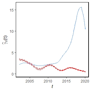
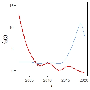
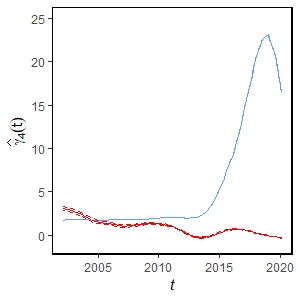
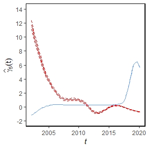
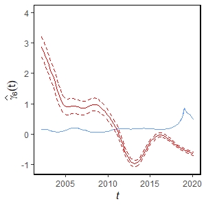
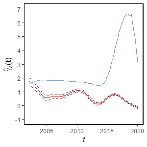
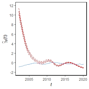
For homophily effects, we first carry out the testing procedure developed in Section 5.1 to test the existence of time-varying trend. The p-value is less than 0.001, which indicates that the homophily effects have significant time evolving trends. We then present the estimated curves of the homophily parameters in Figure 7. It can be seen that if both countries are from America or Europe, they tend to collaborate more frequently. However, two Asian countries are more likely to collaborate in the beginning, but have a lower tendency to collaborate in recent years. Our results differ from those obtained by the method of Kreiß et al., 2019. For example, their method shows that the homophily effects on the collaboration between Asian countries are very close to zero, but our method reveals that the homophily parameter is significantly positive at the very beginning. This can possibly be attributed to the consideration of degree heterogeneity in our method.

7 Discussions

In this article, we proposed a new degree-corrected Cox network model for the analysis of network recurrent data. We developed a kernel smoothing method to estimate the homophily and individual-specific parameters, and established consistency and asymptotic normality of the proposed estimators. We also proposed testing procedures to test for trend and degree heterogeneity in dynamic networks. Although we focus on directed networks, the methods developed here can be easily adapted into undirected networks. Numerical studies demonstrated that the proposed method performed well in practice.

There are several directions for future research. First, the degree heterogeneity we addressed in this paper may be incorporated into other models as well. For example, to model the dependence structure in network settings, the concept of asymptotic uncorrelation was proposed by Kreiß et al., 2019, and further extended to momentary-mm-dependence and β\beta-mixing in Kreiß, 2021. See more related work in Sit et al., 2021 and Kreiß, 2021. However, the degree heterogeneity, which has not been considered in these papers, makes the mathematics behind these types of analysis significantly more challenging with 2​n2n parameters. It would be of interest to explore this in the future.

Second, we only used the local constant fitting to construct the estimating equation for simplicity. Indeed, it can be extended to local linear fitting and general local polynomial fitting. However, the resulting inference procedures would be much more complicated and need future research. Finally, we chose the bandwidth by the rule of thumb. Developing data-driven methods, such as the KK-fold cross-validation, to select the optimal bandwidth is certainly of interest. However, it poses challenges with 2​n2n individual-specific parameters under our model, which requires more effort to study in the future.

References

  • Butts, (2008) Butts, C. T. (2008). A relational event framework for social action. Sociological Methodology, 38, 155–200.
  • Chatterjee et al., (2011) Chatterjee, S., Diaconis, P., and Sly, A. (2011). Random graphs with a given degree sequence. The Annals of Applied Probability, 21, 1400–1435.
  • De Choudhury et al., (2010) De Choudhury, M., Mason, W. A., Hofman, J. M., and Watts, D. J. (2010). Inferring Relevant Social Networks from Interpersonal Communication, page 301–310. Association for Computing Machinery, New York, NY, USA.
  • DuBois et al., (2013) DuBois, C., Butts, C., and Smyth, P. (2013). Stochastic blockmodeling of relational event dynamics. In Proceedings of the Sixteenth International Conference on Artificial Intelligence and Statistics, volume 31 of Proceedings of Machine Learning Research, pages 238–246.
  • Dzemski, (2017) Dzemski, A. (2017). An empirical model of dyadic link formation in a network with unobserved heterogeneity. Working Papers in Economics, page No. 698.
  • Fan and Gijbels, (1996) Fan, J. and Gijbels, I. (1996). Local Polynomial Modelling and Its Applications. Chapman and Hall, London.
  • Fernández-Val and Weidner, (2016) Fernández-Val, I. and Weidner, M. (2016). Individual and time effects in nonlinear panel models with large n, t. Journal of Econometrics, 192, 291–312.
  • Fienberg, (2012) Fienberg, S. E. (2012). A brief history of statistical models for network analysis and open challenges. Journal of Computational and Graphical Statistics, 21, 825–839.
  • Fleming and Harrington, (1991) Fleming, T. R. and Harrington, D. P. (1991). Counting Processes and Survival Analysis. Wiley, New York.
  • Goldenberg et al., (2010) Goldenberg, A., Zheng, A., Fienberg, S. E., and Edoardo, M. A. (2010). A survey of statistical network models. Foundations and Trends in Machine Learning, 2, 129–233.
  • Graham, (2017) Graham, B. S. (2017). An econometric model of network formation with degree heterogeneity. Econometrica, 85, 1033–1063.
  • Hanneke et al., (2010) Hanneke, S., Fu, W., and Xing, E. P. (2010). Discrete temporal models of social networks. Electronic Journal of Statistics, 4, 585–605.
  • Holland and Leinhardt, (1981) Holland, P. W. and Leinhardt, S. (1981). An exponential family of probability distributions for directed graphs. Journal of the American Statistical Association, 76(373), 33–50.
  • Kantorovich, (1948) Kantorovich, L. V. (1948). Functional analysis and applied mathematics. Uspekhi Mat Nauk, pages 89–185.
  • Kantorovich and Akilov, (1964) Kantorovich, L. V. and Akilov, G. P. (1964). Functional Analysis in Normed Spaces. Oxford, Pergamon.
  • Kolaczyk, (2009) Kolaczyk, E. D. (2009). Statistical analysis of network data. Springer-Verlag, New York.
  • Kreiß, (2021) Kreiß, A. (2021). Correlation bounds, mixing and m-dependence under random time-varying network distances with an application to Cox-processes. Bernoulli, 27, 1666 – 1694.
  • Kreiß et al., (2019) Kreiß, A., Mammen, E., and Polonik, W. (2019). Nonparametric inference for continuous-time event counting and link-based dynamic network models. Electronic Journal of Statistics, 13, 2764–2829.
  • Krivitsky and Handcock, (2014) Krivitsky, P. N. and Handcock, M. S. (2014). A separable model for dynamic networks. Journal of the Royal Statistical Society: Series B (Statistical Methodology), 76, 29–46.
  • Lin et al., (1994) Lin, D. Y., Fleming, T. R., and Wwi, L. J. (1994). Confidence bands for survival curves under the proportional hazards model. Biometrika, 81, 73–81.
  • Matias and Miele, (2017) Matias, C. and Miele, V. (2017). Statistical clustering of temporal networks through a dynamic stochastic block model. Journal of the Royal Statistical Society: Series B (Statistical Methodology), 79, 1119–1141.
  • Matias et al., (2018) Matias, C., Rebafka, T., and Villers, F. (2018). A semiparametric extension of the stochastic block model for longitudinal networks. Biometrika, 105, 665–680.
  • Neyman and Scott, (1948) Neyman, J. and Scott, E. L. (1948). Consistent estimates based on partially consistent observations. Econometrica, 16, 1–32.
  • Pensky, (2019) Pensky, M. (2019). Dynamic network models and graphon estimation. The Annals of Statistics, 47, 2378–2403.
  • Perry and Wolfe, (2013) Perry, P. O. and Wolfe, P. J. (2013). Point process modelling for directed interaction networks. Journal of the Royal Statistical Society: Series B (Statistical Methodology), 75, 821–849.
  • Sengupta and Chen, (2018) Sengupta, S. and Chen, Y. (2018). A block model for node popularity in networks with community structure. Journal of the Royal Statistical Society: Series B (Statistical Methodology), 80(2), 365–386.
  • (27) Sewell, D. K. and Chen, Y. (2015a). Analysis of the formation of the structure of social networks by using latent space models for ranked dynamic networks. Journal of the Royal Statistical Society: Series C (Applied Statistics), 64, 611–633.
  • (28) Sewell, D. K. and Chen, Y. (2015b). Latent space models for dynamic networks. Journal of the American Statistical Association, 110, 1646–1657.
  • Sit et al., (2021) Sit, T., Ying, Z., and Yu, Y. (2021). Event history analysis of dynamic networks. Biometrika, 108, 223–230.
  • Vu et al., (2011) Vu, D. Q., Asuncion, A. U., Hunter, D., and Smyth, P. (2011). Dynamic egocentric models for citation networks. In Proceedings of the 28th International Conference on Machine Learning (ICML-11), pages 857–864.
  • Yan et al., (2019) Yan, T., Jiang, B., Fienberg, S. E., and Leng, C. (2019). Statistical inference in a directed network model with covariates. Journal of the American Statistical Association, 114, 857–868.
  • (32) Yan, T., Leng, C., and Zhu, J. (2016a). Asymptotics in directed exponential random graph models with an increasing bi-degree sequence. The Annals of Statistics, 44, 31–57.
  • (33) Yan, T., Leng, C., and Zhu, J. (2016b). Asymptotics in directed exponential random graph models with an increasing bi-degree sequence. The Annals of Statistics, 44(1), 31–57.
  • Yang et al., (2011) Yang, T., Chi, Y., Zhu, S., Gong, Y., and Jin, R. (2011). Detecting communities and their evolutions in dynamic social networks-a Bayesian approach. Machine learning, 82, 157–189.

Table 1: The MISEs for parameters α1∗​(t),αn/2+1∗​(t),β1∗​(t),βn/2+1∗​(t)\alpha_{1}^{*}(t),\alpha_{n/2+1}^{*}(t),\beta_{1}^{*}(t),\beta_{n/2+1}^{*}(t) and γ1∗​(t)\gamma_{1}^{*}(t).
nn MISE
α1∗​(t)\alpha_{1}^{*}(t) αn/2+1∗​(t)\alpha_{n/2+1}^{*}(t) β1∗​(t)\beta_{1}^{*}(t) βn/2+1∗​(t)\beta_{n/2+1}^{*}(t) γ1∗​(t)\gamma_{1}^{*}(t)
100100 0.129 0.190 0.130 0.169 0.008
200200 0.111 0.173 0.107 0.153 0.004
500500 0.104 0.169 0.096 0.149 0.002

Table 2: The coverage probability for parameters ×100\times 100 (the length of 95% confidence interval) for α1∗​(t),αn/2+1∗​(t),β1∗​(t),βn/2+1∗​(t)\alpha_{1}^{*}(t),\alpha_{n/2+1}^{*}(t),\beta_{1}^{*}(t),\beta_{n/2+1}^{*}(t) and γ1∗​(t)\gamma_{1}^{*}(t) at different time points.
   nn       t=0.4t=0.4       t=0.6t=0.6       t=0.8t=0.8   
   100100       α1∗​(t)\alpha_{1}^{*}(t)       95.5 (1.00)       92.3 (1.61)       95.9 (1.45)   
   αn/2+1∗​(t)\alpha_{n/2+1}^{*}(t)       93.7 (1.64)       93.8 (1.69)       95.4 (1.39)   
   β1∗​(t)\beta_{1}^{*}(t)       92.8 (1.12)       95.8 (1.60)       92.7 (1.30)   
   βn/2+1∗​(t)\beta_{n/2+1}^{*}(t)       92.6 (1.18)       94.7 (1.65)       93.9 (1.66)   
   γ1∗​(t)\gamma_{1}^{*}(t)       93.8 (0.31)       95.8 (0.44)       94.7 (0.37)   
   200200       α1∗​(t)\alpha_{1}^{*}(t)       96.5 (0.95)       97.8 (1.54)       91.1 (1.36)   
   αn/2+1∗​(t)\alpha_{n/2+1}^{*}(t)       95.8 (1.65)       95.3 (1.63)       95.9 (1.29)   
   β1∗​(t)\beta_{1}^{*}(t)       90.7 (1.08)       92.3 (1.57)       94.4 (1.20)   
   βn/2+1∗​(t)\beta_{n/2+1}^{*}(t)       96.1 (1.15)       96.3 (1.61)       95.5 (1.60)   
   γ1∗​(t)\gamma_{1}^{*}(t)       95.3 (0.23)       95.3 (0.33)       95.3 (0.27)   
   500500       α1∗​(t)\alpha_{1}^{*}(t)       95.5 (0.92)       97.1 (1.53)       94.8 (1.33)   
   αn/2+1∗​(t)\alpha_{n/2+1}^{*}(t)       92.9 (1.73)       94.5 (1.65)       93.7 (1.24)   
   β1∗​(t)\beta_{1}^{*}(t)       93.7 (1.08)       94.9 (1.60)       93.8 (1.14)   
   βn/2+1∗​(t)\beta_{n/2+1}^{*}(t)       95.5 (1.15)       97.5 (1.54)       95.4 (1.59)   
   γ1∗​(t)\gamma_{1}^{*}(t)       94.6 (0.16)       95.3 (0.23)       95.2 (0.19)   
Refer to caption
(a) n=100n=100, α^1​(t)\widehat{\alpha}_{1}(t)
Refer to caption
(b) n=100n=100, β^1​(t)\widehat{\beta}_{1}(t)
Refer to caption
(c) n=100n=100, γ^1​(t)\widehat{\gamma}_{1}(t)
Refer to caption
(d) n=200n=200, α^1​(t)\widehat{\alpha}_{1}(t)
Refer to caption
(e) n=200n=200, β^1​(t)\widehat{\beta}_{1}(t)
Refer to caption
(f) n=200n=200, γ^1​(t)\widehat{\gamma}_{1}(t)
Refer to caption
(g) n=500n=500, α^1​(t)\widehat{\alpha}_{1}(t)
Refer to caption
(h) n=500n=500, β^1​(t)\widehat{\beta}_{1}(t)
Refer to caption
(i) n=500n=500, γ^1​(t)\widehat{\gamma}_{1}(t)
Figure 1: The estimated curves for α1∗​(t),β1∗​(t)\alpha_{1}^{*}(t),~\beta_{1}^{*}(t) and γ1∗​(t).\gamma_{1}^{*}(t). The black solid lines denote the true curves of α1∗​(t),β1∗​(t)\alpha_{1}^{*}(t),~\beta_{1}^{*}(t) and γ1∗​(t).\gamma_{1}^{*}(t). The red solid lines are the averages (over 1000 replications) of the proposed estimators α^1​(t),β^1​(t)\widehat{\alpha}_{1}(t),~\widehat{\beta}_{1}(t) and γ^1​(t)\widehat{\gamma}_{1}(t), while the red dashed lines represent the pointwise 95%95\% confidence intervals.
Refer to caption
(a) b=0b=0
Refer to caption
(b) b=1/3b=1/3
Refer to caption
(c) b=1/2b=1/2
Refer to caption
(d) b=1b=1
Figure 2: The red solid lines are the average of the proposed estimators of γ∗​(t)\gamma^{*}(t) over 1000 replications, and the red dashed lines are the pointwise 95%95\% confidence intervals. The blue solid lines are the average of the estimators obtained by the method of Kreiß et al., 2019 over 1000 replications, and the blue dashed lines are the pointwise 95%95\% confidence intervals. The black solid lines represent the true curves of γ∗​(t).\gamma^{*}(t).
Refer to caption
(a) Size and power of 𝒯η\mathcal{T}_{\eta}
Refer to caption
(b) Size and power of 𝒯γ\mathcal{T}_{\gamma}
Figure 3: The size and power of the test statistics 𝒯η\mathcal{T}_{\eta} and 𝒯γ\mathcal{T}_{\gamma} as trending levels c~1\widetilde{c}_{1} and c~2\widetilde{c}_{2} increase.
Refer to caption
(a)
Figure 4: The size and power of the test statistic 𝒟α\mathcal{D}_{\alpha} as the heterogeneity level c~\widetilde{c} varies from 0 to 1.5.
Refer to caption
(a) Jan. 2000 - Apr. 2002 (P1)
Refer to caption
(b) May. 2002 - Aug. 2004 (P2)
Refer to caption
(c) Sep. 2004 - Jan. 2007 (P3)
Refer to caption
(d) Feb. 2007 - May. 2009 (P4)
Figure 5: The collaboration links of 74 countries from Jan. 2000 to May. 2009. The size of nodes corresponds to their in-degrees. The countries are color coded by continent: America (orange), Asia (cyan), Europe (green), Oceania (yellow) and Africa (dark blue).
Refer to caption
(a) Chad, α^′(t)\widehat{\alpha}^{{}^{\prime}}(t)
Refer to caption
(b) Chad, β^′(t)\widehat{\beta}^{{}^{\prime}}(t)
Refer to caption
(c) USA, α^′(t)\widehat{\alpha}^{{}^{\prime}}(t)
Refer to caption
(d) USA, β^′(t)\widehat{\beta}^{{}^{\prime}}(t)
Refer to caption
(e) Nigeria, α^′(t)\widehat{\alpha}^{{}^{\prime}}(t)
Refer to caption
(f) Nigeria, β^′(t)\widehat{\beta}^{{}^{\prime}}(t)
Figure 6: Real data analysis: Estimation results of degree heterogeneity parameters. The solid lines are the estimated curves, and the dashed lines denote their 95%95\% pointwise confidence bands.
Refer to caption
(a) γ^1​(t)\widehat{\gamma}_{1}(t) for covariate Mi​MjM_{i}M_{j}
Refer to caption
(b) γ^2​(t)\widehat{\gamma}_{2}(t) for covariate Mi​AjM_{i}A_{j}
Refer to caption
(c) γ^3​(t)\widehat{\gamma}_{3}(t) for covariate Mi​EjM_{i}E_{j}
Refer to caption
(d) γ^4​(t)\widehat{\gamma}_{4}(t) for covariate Ai​MjA_{i}M_{j}
Refer to caption
(e) γ^5​(t)\widehat{\gamma}_{5}(t) for covariate Ai​AjA_{i}A_{j}
Refer to caption
(f) γ^6​(t)\widehat{\gamma}_{6}(t) for covariate Ai​EjA_{i}E_{j}
Refer to caption
(g) γ^7​(t)\widehat{\gamma}_{7}(t) for covariate Ei​MjE_{i}M_{j}
Refer to caption
(h) γ^8​(t)\widehat{\gamma}_{8}(t) for covariate Ei​AjE_{i}A_{j}
Refer to caption
(i) γ^9​(t)\widehat{\gamma}_{9}(t) for covariate Ei​EjE_{i}E_{j}
Figure 7: Real data analysis: Estimation results of homophily parameters. The red solid lines represent our estimates and red dashed lines are their 95%95\% pointwise confidence bands. The blue lines are estimates obtained by the method of Kreiß et al., 2019.

Supplementary Material for “A degree-corrected Cox model for dynamic networks”

Appendix A Preliminaries

In this section, we present some results that will be used in the proofs and state them as lemmas. Given bLb_{L}, bU>0b_{U}>0, we say M=(mi,j)n×nM=(m_{i,j})_{n\times n} belongs to the matrix class ℒn​(bL,bU)\mathcal{L}_{n}(b_{L},b_{U}) if MM satisfies

mi,j=mj,i=0,i,j=1,…,n,i≠j,mi,j=mj,i=0,i,j=n+1,…,2​n−1,i≠j,mn+i,i=mi,n+i=0,i,j=1,…,n−1,bL≤mi,i−∑j=n+12​n−1mi,j≤bU,i=1,…,n,mi,i=∑k=1nmk,i=∑k=1nmi,k,i=n+1,…,2n−1,bL≤mi,j=mj,i≤bU,i=1,…,n,j=n+1,…,2n−1;j≠n+i.\begin{array}[]{l}m_{i,j}=m_{j,i}=0,~~i,j=1,\dots,n,~i\neq j,\\ m_{i,j}=m_{j,i}=0,~~i,j=n+1,\dots,2n-1,~i\neq j,\\ m_{n+i,i}=m_{i,n+i}=0,~~i,j=1,\dots,n-1,\\ b_{L}\leq m_{i,i}-\sum_{j=n+1}^{2n-1}m_{i,j}\leq b_{U},~~i=1,\dots,n,\\ m_{i,i}=\sum_{k=1}^{n}m_{k,i}=\sum_{k=1}^{n}m_{i,k},~~i=n+1,\dots,2n-1,\\ b_{L}\leq m_{i,j}=m_{j,i}\leq b_{U},~~i=1,\ldots,n,~j=n+1,\dots,2n-1;~j\neq n+i.\end{array} (A.1)

Clearly, if M∈ℒn​(bL,bU)M\in\mathcal{L}_{n}(b_{L},b_{U}), then MM is a (2​n−1)×(2​n−1)(2n-1)\times(2n-1) diagonally dominant, symmetric nonnegative matrix and MM has the following structure:

M=(M11M12M12⊤M22),M=\left(\begin{array}[]{ll}M_{11}&M_{12}\\ M_{12}^{\top}&M_{22}\end{array}\right),

where M11M_{11} (nn by nn) and M22M_{22} (n−1n-1 by n−1n-1) are diagonal matrices, M12M_{12} (n−1n-1 by nn) is a nonnegative matrix whose non-diagonal elements are positive and diagonal elements equal to zero. Here, the diagonal elements of M12M_{12} refer to elements whose row and column indices are the same. Generally, the inverse of MM does not have a closed form. Define m2​n,i=mi,2​n:=mi,i−∑j=1;j≠i2​n−1mi,jm_{2n,i}=m_{i,2n}:=m_{i,i}-\sum_{j=1;j\neq i}^{2n-1}m_{i,j} for i=1,…,2​n−1i=1,\ldots,2n-1 and m2​n,2​n=∑i=12​n−1m2​n,im_{2n,2n}=\sum_{i=1}^{2n-1}m_{2n,i}. Then bL≤m2​n,i≤bUb_{L}\leq m_{2n,i}\leq b_{U} for i=1,…,n−1i=1,\ldots,n-1, m2​n,i=0m_{2n,i}=0 for i=n,n+1,…,2​n−1i=n,n+1,\ldots,2n-1 and m2​n,2​n=∑i=1nmi,2​n=∑i=1nm2​n,im_{2n,2n}=\sum_{i=1}^{n}m_{i,2n}=\sum_{i=1}^{n}m_{2n,i}. Yan et al. 2016 proposed to use a simple matrix 𝒮⁡(M)=(si​j)(2​n−1)×(2​n−1)\mathcal{S}(M)=(s_{ij})_{(2n-1)\times(2n-1)} to approximate the inverse of M∈ℒn​(bL,bM)M\in\mathcal{L}_{n}(b_{L},b_{M}), where si​js_{ij} is defined as

si,j={δi,jmi,i+1m2​n,2​n,i,j=1,…,n,−1m2​n,2​n,i=1,…,n,j=n+1,…,2​n−1,−1m2​n,2​n,i=n+1,…,2​n−1,j=1,…,n,δi,jmi,i+1m2​n,2​n,i,j=n+1,…,2​n−1.s_{i,j}=\left\{\begin{array}[]{ll}\frac{\delta_{i,j}}{m_{i,i}}+\frac{1}{m_{2n,2n}},&i,j=1,\ldots,n,\\ -\frac{1}{m_{2n,2n}},&i=1,\ldots,n,~~j=n+1,\ldots,2n-1,\\ -\frac{1}{m_{2n,2n}},&i=n+1,\ldots,2n-1,~~j=1,\ldots,n,\\ \frac{\delta_{i,j}}{m_{i,i}}+\frac{1}{m_{2n,2n}},&i,j=n+1,\ldots,2n-1.\end{array}\right.

In the above equation, δi,j=1\delta_{i,j}=1 when i=ji=j and δi,j=0\delta_{i,j}=0 when i≠ji\neq j.

Define ‖M‖max:=maxi,j⁡|mi,j|\|M\|_{\max}:=\max_{i,j}|m_{i,j}| as the maximum absolute entry-wise norm for any matrix M=(ai,j).M=(a_{i,j}). Yan et al., 2016a proved that the upper bound of the approximation error has an order n−2n^{-2}.

Lemma 1 (Proposition 1 in Yan et al. 2016).

If M∈ℒn​(bL,bU)M\in\mathcal{L}_{n}(b_{L},b_{U}) with bU/bL=o⁡(n)b_{U}/b_{L}=o(n), then for large enough nn,

‖M−1−𝒮⁡(M)‖max≤c1​bU2bL3​(n−1)2,\|M^{-1}-\mathcal{S}(M)\|_{\max}\leq\frac{c_{1}b_{U}^{2}}{b_{L}^{3}(n-1)^{2}},

where c1c_{1} is a constant that does not depend on MM, mm and nn.

Let G⁡(x):ℝn→ℝnG(x):\mathbb{R}^{n}\to\mathbb{R}^{n} be a function vector on x∈ℝnx\in\mathbb{R}^{n}. We say that a Jacobian matrix G(1)​(x)G^{(1)}(x) with x∈ℝnx\in\mathbb{R}^{n} is Lipschitz continuous on a convex set 𝒟⊂ℝn\mathcal{D}\subset\mathbb{R}^{n} if for any x,y∈𝒟x,y\in\mathcal{D}, there exists a constant λ>0\lambda>0, such that for any vector v∈ℝnv\in\mathbb{R}^{n}, the inequality

‖{G(1)​(x)−G(1)​(y)}​v‖∞≤λ​‖x−y‖∞​‖v‖∞\|\left\{G^{(1)}(x)-G^{(1)}(y)\right\}v\|_{\infty}\leq\lambda\|x-y\|_{\infty}\|v\|_{\infty}

holds.

We introduce an error bound in the Newton method by Kantorovich and Akilov, 1964 under the Kantorovich conditions (Kantorovich, 1948).

Lemma 2 (Theorem 6 in Kantorovich and Akilov, 1964).

Let 𝒟\mathcal{D} be an open convex subset of ℝn\mathbb{R}^{n} and F:𝒟→ℝnF:\mathcal{D}\to\mathbb{R}^{n} be Fréchet differentiable. Assume that, at some x0∈𝒟{x}_{0}\in\mathcal{D}, F′​(x0)F^{\prime}({x}_{0}) is invertible and that

‖F′​(x0)−1​(F′​(x)−F′​(y))‖≤K​‖x−y‖,x,y∈𝒟,\displaystyle\|F^{\prime}({x}_{0})^{-1}(F^{\prime}({x})-F^{\prime}({y}))\|\leq K\|{x}-{y}\|,~~{x},{y}\in\mathcal{D}, (9)
‖F′​(x0)−1​F​(x0)‖≤η,h=K​η≤1/2,\displaystyle\|F^{\prime}({x}_{0})^{-1}F({x}_{0})\|\leq\eta,~~h=K\eta\leq 1/2, (10)
S¯​(x0,t∗)⊆𝒟,t∗=2​η/(1+1−2​h).\displaystyle\bar{S}({x}_{0},t^{*})\subseteq\mathcal{D},~~t^{*}=2\eta/(1+\sqrt{1-2h}).

Then: (1) The Newton iterates xn+1=xn−{F′​(xn)}−1​F​(xn){x}_{n+1}={x}_{n}-\{F^{\prime}({x}_{n})\}^{-1}F({x}_{n}), n≥0n\geq 0, are well-defined, lie in S¯​(x0,t∗)\bar{S}({x}_{0},t^{*}) and converge to a solution x∗{x}^{*} of F⁡(x)=0F({x})=0.
(2) The solution x∗{x}^{*} is unique in S⁡(x0,t∗⁣∗)∩𝒟S({x}_{0},t^{**})\cap\mathcal{D}, t∗⁣∗=(1+1−2​h)/Kt^{**}=(1+\sqrt{1-2h})/K if 2​h<12h<1 and in S¯​(x0,t∗⁣∗)\bar{S}({x}_{0},t^{**}) if 2​h=12h=1.
(3) ‖x∗−xn‖≤t∗\|{x}^{*}-{x}_{n}\|\leq t^{*} if n=0n=0 and ‖x∗−xn‖≤21−n​(2​h)2n−1​η\|{x}^{*}-{x}_{n}\|\leq 2^{1-n}(2h)^{2^{n}-1}\eta if n≥1n\geq 1.

The following lemma gives an exponential bound for the moment of a bounded random variable.

Lemma 3.

Let YY be a random variable. If |Y|<C0|Y|<C_{0} for some constant C0C_{0} and 𝔼⁡(Y)=0,\mathbb{E}(Y)=0, then for all sufficiently small υ>0,\upsilon>0,

𝔼⁡{exp⁡(υ​Y)}≤exp⁡{υ2​𝔼​(Y2)}.\mathbb{E}\{\exp(\upsilon Y)\big\}\leq\exp\big\{\upsilon^{2}\mathbb{E}(Y^{2})\big\}.
Proof.

By Taylor’s expansion, for a small υ>0\upsilon>0, we have

𝔼​{exp⁡(υ​Y)}=\displaystyle\mathbb{E}\big\{\exp(\upsilon Y)\big\}= 1+υ​𝔼​(Y)+12​υ2​𝔼​(Y2)+∑j=3∞υj​𝔼​Yjj!\displaystyle 1+\upsilon\mathbb{E}(Y)+\frac{1}{2}\upsilon^{2}\mathbb{E}(Y^{2})+\sum_{j=3}^{\infty}\frac{\upsilon^{j}\mathbb{E}Y^{j}}{j!}
≤\displaystyle\leq 1+12​υ2​𝔼​(Y2)+υ2​𝔼​Y22​∑j=3∞υj−2​C0j−23j−2\displaystyle 1+\frac{1}{2}\upsilon^{2}\mathbb{E}(Y^{2})+\frac{\upsilon^{2}\mathbb{E}Y^{2}}{2}\sum_{j=3}^{\infty}\frac{\upsilon^{j-2}C_{0}^{j-2}}{3^{j-2}}
=\displaystyle= 1+12​υ2​𝔼​(Y2)+υ2​𝔼​Y22​υ​C0/31−υ​C0/3.\displaystyle 1+\frac{1}{2}\upsilon^{2}\mathbb{E}(Y^{2})+\frac{\upsilon^{2}\mathbb{E}Y^{2}}{2}\frac{\upsilon C_{0}/3}{1-\upsilon C_{0}/3}.

By choosing 0<υ<min⁡{1,2​C0/3},0<\upsilon<\min\{1,2C_{0}/3\}, we obtain

1+12​υ2​𝔼​(Y2)+υ2​𝔼​Y22​υ​C0/31−υ​C0/3≤1+υ2​𝔼​(Y2)≤exp⁡{υ2​𝔼​(Y2)},\displaystyle 1+\frac{1}{2}\upsilon^{2}\mathbb{E}(Y^{2})+\frac{\upsilon^{2}\mathbb{E}Y^{2}}{2}\frac{\upsilon C_{0}/3}{1-\upsilon C_{0}/3}\leq 1+\upsilon^{2}\mathbb{E}(Y^{2})\leq\exp\Big\{\upsilon^{2}\mathbb{E}(Y^{2})\Big\},

where the last inequality holds for all small υ>0.\upsilon>0. This completes the proof. ∎

Appendix B Proofs of Theorems 1-3

B.1 Proof of Theorem 1

In this section, we present the proof of Theorem 1. We first prove three lemmas. The first lemma is about the upper bounds of ‖F∗​(t)‖∞\|F^{*}(t)\|_{\infty} and ‖Q∗​(t)‖∞\|Q^{*}(t)\|_{\infty}, where F∗​(t)=F⁡(θ∗​(t))F^{*}(t)=F(\theta^{*}(t)) and Q∗​(t)=Q⁡(θ∗​(t))Q^{*}(t)=Q(\theta^{*}(t)). For a given γ⁡(t)\gamma(t), write

Fγ​(η⁡(t))=(F1,γ​(η⁡(t)),…,F2​n−1,γ​(η⁡(t)))⊤=F⁡(η⁡(t),γ⁡(t)).F_{\gamma}(\eta(t))=(F_{1,\gamma}(\eta(t)),\dots,F_{2n-1,\gamma}(\eta(t)))^{\top}=F(\eta(t),\gamma(t)).

Define αi,γ∗​(t)\alpha_{i,\gamma}^{*}(t) and βj,γ∗​(t)\beta_{j,\gamma}^{*}(t) as the solution to 𝔼⁡{ℳi​j​(t,αi​(t),βj​(t),γ⁡(t))}=0​(1≤i≠j≤n)\mathbb{E}\{\mathcal{M}_{ij}(t;\alpha_{i}(t),\beta_{j}(t),\gamma(t))\}=0~(1\leq i\neq j\leq n) with a given γ⁡(t).\gamma(t). Further define ηγ∗​(t)=(α1,γ∗​(t),…,αn,γ∗​(t),β1,γ∗​(t),…,βn,γ∗​(t))⊤.\eta^{*}_{\gamma}(t)=(\alpha_{1,\gamma}^{*}(t),\dots,\alpha_{n,\gamma}^{*}(t),\beta_{1,\gamma}^{*}(t),\dots,\beta_{n,\gamma}^{*}(t))^{\top}.

Lemma 4.

Suppose Conditions 1-5 holds, and γ⁡(t)\gamma(t) takes values in a compact set 𝒥\mathcal{J} of ℝp.\mathbb{R}^{p}. Then we have

supt∈[a,b]‖F∗​(t)‖∞\displaystyle\sup_{t\in[a,b]}\|F^{*}(t)\|_{\infty} =\displaystyle= Op​((qn+1)​eqn​log⁡n​h1n​h1),\displaystyle O_{p}\Big((q_{n}+1)e^{q_{n}}\sqrt{\frac{\log nh_{1}}{nh_{1}}}\Big), (11)
supt∈[a,b]‖Q∗​(t)‖∞\displaystyle\sup_{t\in[a,b]}\|Q^{*}(t)\|_{\infty} =\displaystyle= Op​(κn​(qn+1)​eqn​log⁡N​h2N​h2),\displaystyle O_{p}\Big(\kappa_{n}(q_{n}+1)e^{q_{n}}\sqrt{\frac{\log Nh_{2}}{Nh_{2}}}\Big), (12)
supt∈[a,b]supγ⁡(t)∈𝒥‖Fγ​(ηγ∗​(t))‖∞\displaystyle\sup_{t\in[a,b]}\sup_{\gamma(t)\in\mathcal{J}}\|F_{\gamma}(\eta_{\gamma}^{*}(t))\|_{\infty} =\displaystyle= Op​((qn+1)​eqn​log⁡n​h1n​h1).\displaystyle O_{p}\Big((q_{n}+1)e^{q_{n}}\sqrt{\frac{\log nh_{1}}{nh_{1}}}\Big). (13)
Proof.

For easy exposition, define

πi​j∗​(t)\displaystyle\pi_{ij}^{*}(t) =\displaystyle= αi∗​(t)+βj∗​(t)+Zi​j​(t)⊤​γ∗​(t),\displaystyle\alpha_{i}^{*}(t)+\beta_{j}^{*}(t)+Z_{ij}(t)^{\top}\gamma^{*}(t),
π1,i​j∗​(t)\displaystyle\pi_{1,ij}^{*}(t) =\displaystyle= αi∗​(t)+Zi​j​(t)⊤​γ∗​(t),\displaystyle\alpha_{i}^{*}(t)+Z_{ij}(t)^{\top}\gamma^{*}(t),
π2,i​j∗​(t)\displaystyle\pi_{2,ij}^{*}(t) =\displaystyle= βj∗​(t)+Zi​j​(t)⊤​γ∗​(t).\displaystyle\beta_{j}^{*}(t)+Z_{ij}(t)^{\top}\gamma^{*}(t).

Similarly, define

πi​j∗​(s,t)\displaystyle\pi_{ij}^{*}(s,t) =\displaystyle= αi∗​(t)+βj∗​(t)+Zi​j​(s)⊤​γ∗​(t),\displaystyle\alpha_{i}^{*}(t)+\beta_{j}^{*}(t)+Z_{ij}(s)^{\top}\gamma^{*}(t),
π1,i​j∗​(s,t)\displaystyle\pi_{1,ij}^{*}(s,t) =\displaystyle= αi∗​(t)+Zi​j​(s)⊤​γ∗​(t),\displaystyle\alpha_{i}^{*}(t)+Z_{ij}(s)^{\top}\gamma^{*}(t),
π2,i​j∗​(s,t)\displaystyle\pi_{2,ij}^{*}(s,t) =\displaystyle= βj∗​(t)+Zi​j​(s)⊤​γ∗​(t).\displaystyle\beta_{j}^{*}(t)+Z_{ij}(s)^{\top}\gamma^{*}(t).

For i=1,…,ni=1,\ldots,n, we decompose (n−1)​Fi∗​(t)(n-1)F_{i}^{*}(t) into two parts:

(n−1)​Fi∗​(t)=∑j≠i∫0τ𝒦h1​(s−t)​d​ℳi​j​(s)⏟B1​i​(t)−∑j≠i∫0τKh1​(s−t)​[eπ1,i​j∗​(s,t)−eπ1,i​j∗​(s)]​ds⏟B2​i​(t).(n-1)F_{i}^{*}(t)=\underbrace{\sum_{j\neq i}\int_{0}^{\tau}\mathcal{K}_{h_{1}}(s-t)d\mathcal{M}_{ij}(s)}_{B_{1i}(t)}-\underbrace{\sum_{j\neq i}\int_{0}^{\tau}K_{h_{1}}(s-t)\big[e^{\pi_{1,ij}^{*}(s,t)}-e^{\pi_{1,ij}^{*}(s)}\big]ds}_{B_{2i}(t)}. (14)

Note that if g⁡(t)g(t) is a generic function with second derivatives bounded above by a constant cc, we have (e.g., Eubank 1988, Eubank 1988, p.128)

|∫0τ𝒦h1​(s−t)​[g⁡(s)−g⁡(t)]​𝑑s|≤12​c​h12,\displaystyle\Big|\int_{0}^{\tau}\mathcal{K}_{h_{1}}(s-t)[g(s)-g(t)]ds\Big|\leq\frac{1}{2}ch_{1}^{2},

where t∈[h1,τ−h1]t\in[h_{1},\tau-h_{1}] and h1h_{1} satisfies [−1,1]⊂[−t/h1,(τ−t)/h1][-1,1]\subset[-t/h_{1},(\tau-t)/h_{1}]. It follows from Conditions 1, 2 and 4 that

|𝔼​B2​i​(t)|=|∑j≠i𝔼⁡{∫0τ𝒦h1​(s−t)​[eπi​j∗​(s,t)−eπi​j∗​(s)]​𝑑s}|=O⁡(eqn​n​h12)\displaystyle|\mathbb{E}B_{2i}(t)|=\bigg|\sum_{j\neq i}\mathbb{E}\Bigg\{\int_{0}^{\tau}\mathcal{K}_{h_{1}}(s-t)\big[e^{\pi_{ij}^{*}(s,t)}-e^{\pi_{ij}^{*}(s)}\big]ds\Bigg\}\bigg|=O\big(e^{q_{n}}nh_{1}^{2}\big)

and

Var​(B2​i​(t))≤∑j≠i𝔼​[∫0τ𝒦h1​(s−t)​[eπi​j∗​(s,t)​𝑑s−eπi​j​(s)]​𝑑s]2=O⁡(e2​qn​n​h14),\displaystyle\text{Var}(B_{2i}(t))\leq\sum_{j\neq i}\mathbb{E}\Bigg[\int_{0}^{\tau}\mathcal{K}_{h_{1}}(s-t)\big[e^{\pi_{ij}^{*}(s,t)}ds-e^{\pi_{ij}(s)}\big]ds\Bigg]^{2}=O\big(e^{2q_{n}}nh_{1}^{4}\big),

where f(l)​(t)f^{(l)}(t) denotes the llth-order derivative of any function f⁡(t)f(t). By Chebyshev’s inequality, we have

B2​i​(t)=Op​(eqn​n​h12).B_{2i}(t)=O_{p}(e^{q_{n}}nh_{1}^{2}). (15)

If n​eqn​h15→0ne^{q_{n}}h_{1}^{5}\rightarrow 0, then

B2​i​(t)=op​(e2​qn​n​log⁡(n​h1)/h1).B_{2i}(t)=o_{p}\left(e^{2q_{n}}\sqrt{n\log(nh_{1})/h_{1}}\right).

By the union bound and the triangle inequality, we have that for sufficiently large nn,

ℙ⁡(supt∈[a,b](n−1)​‖F∗​(t)‖∞≥4​10​C1​ϑn​n​log⁡(n​h1)/h1)\displaystyle\mathbb{P}\Big(\sup_{t\in[a,b]}(n-1)\|F^{*}(t)\|_{\infty}\geq 4\sqrt{10}C_{1}\vartheta_{n}\sqrt{n\log(nh_{1})/h_{1}}\;\Big)
≤\displaystyle\leq (n−1)max1≤i≤n−1ℙ(supt∈[a,b]|B1​i(t)|+supt∈[a,b]|B2​i(t)}|≥410C1ϑnn​log⁡(n​h1)/h1)\displaystyle(n-1)\max_{1\leq i\leq n-1}\mathbb{P}\Big(\sup_{t\in[a,b]}|B_{1i}(t)|+\sup_{t\in[a,b]}|B_{2i}(t)\}|\geq 4\sqrt{10}C_{1}\vartheta_{n}\sqrt{n\log(nh_{1})/h_{1}}\;\Big)
≤\displaystyle\leq (n−1)​max1≤i≤n−1⁡ℙ⁡(supt∈[a,b]|B1​i​(t)|≥2​10​C1​ϑn​n​log⁡(n​h1)/h1),\displaystyle(n-1)\max_{1\leq i\leq n-1}\mathbb{P}\Big(\sup_{t\in[a,b]}|B_{1i}(t)|\geq 2\sqrt{10}C_{1}\vartheta_{n}\sqrt{n\log(nh_{1})/h_{1}}\;\Big), (16)

where C1C_{1} is some constant specified below and ϑn=eqn​(qn+1)>1\vartheta_{n}=e^{q_{n}}(q_{n}+1)>1.

We now bound the probability in (16). For any κ>0\kappa>0, partition [a,b][a,b] into disjoint subsets ⋃k=1MnΘk\bigcup_{k=1}^{M_{n}}\Theta_{k} such that the distance between any two points in Θk\Theta_{k} does not exceed κ​h12\kappa h_{1}^{2}. Note that MnM_{n} is not larger that O⁡(τ/(κ​h12))O(\tau/(\kappa h_{1}^{2})). Then, we have

ℙ⁡(supt∈[a,b]|B1​i​(t)|>ε)≤∑k=1Mnℙ⁡(|B1​i​(tk)|>ε2)+∑k=1Mnℙ⁡(supt∈Θk|B1​i​(t)−B1​i​(tk)|>ε2).\mathbb{P}\Big(\sup_{t\in[a,b]}|B_{1i}(t)|>\varepsilon\Big)\leq\sum_{k=1}^{M_{n}}\mathbb{P}\Big(|B_{1i}(t_{k})|>\frac{\varepsilon}{2}\Big)+\sum_{k=1}^{M_{n}}\mathbb{P}\Big(\sup_{t\in\Theta_{k}}|B_{1i}(t)-B_{1i}(t_{k})|>\frac{\varepsilon}{2}\Big). (17)

Let Y1​i​j​(t)=∫0τ𝒦⁡((s−t)/h1)​d​ℳi​j​(s).Y_{1ij}(t)=\int_{0}^{\tau}\mathcal{K}((s-t)/h_{1})d\mathcal{M}_{ij}(s). By Markov’s inequality and Lemma 3, we have

ℙ⁡(∑j≠iY1​i​j​(tk)>h1​ε/2)\displaystyle\mathbb{P}\Big(\sum_{j\neq i}Y_{1ij}(t_{k})>h_{1}\varepsilon/2\Big)
≤\displaystyle\leq exp{−υh1ε/2}𝔼[exp{υ∑j≠iY1​i​j(tk)}]\displaystyle\exp\{-\upsilon h_{1}\varepsilon/2\}\mathbb{E}\Big[\exp\Big\{\upsilon\sum_{j\neq i}Y_{1ij}(t_{k})\Big\}\Big]
≤\displaystyle\leq exp{−υh1ε/2}∏j≠i𝔼[exp{υY1​i​j(tk)}]\displaystyle\exp\{-\upsilon h_{1}\varepsilon/2\}\prod_{j\neq i}\mathbb{E}\Big[\exp\big\{\upsilon Y_{1ij}(t_{k})\big\}\Big]
≤\displaystyle\leq exp{−υh1ε/2}∏j≠iexp(υ2Var(Y1​i​j(tk)))\displaystyle\exp\{-\upsilon h_{1}\varepsilon/2\}\prod_{j\neq i}\exp\Big(\upsilon^{2}\text{Var}(Y_{1ij}(t_{k}))\Big)

for some small υ>0\upsilon>0. Note that there exists some constant C1>0C_{1}>0 such that |Y1​i​j​(tk)|<C1|Y_{1ij}(t_{k})|<C_{1} and Var​(Y1​i​j​(tk))<C12​ϑn2​h1.\text{Var}(Y_{1ij}(t_{k}))<C_{1}^{2}\vartheta_{n}^{2}h_{1}. Therefore, we have

ℙ(∑j≠iY1​i​j(tk)>h1ε/2)≤exp(−υh1ε/2+C12υ2nϑnh1).\mathbb{P}\Big(\sum_{j\neq i}Y_{1ij}(t_{k})>h_{1}\varepsilon/2\Big)\leq\exp\Big(-\upsilon h_{1}\varepsilon/2+C_{1}^{2}\upsilon^{2}n\vartheta_{n}h_{1}\Big).

Then, by setting ε=2​10​C1​ϑn​n​log⁡(n​h1)/h1\varepsilon=2\sqrt{10}C_{1}\vartheta_{n}\sqrt{n\log(nh_{1})/h_{1}} and υ=ε/(4​C12​ϑn2​n),\upsilon=\varepsilon/(4C_{1}^{2}\vartheta_{n}^{2}n), we have

ℙ(|B1​i(tj)|>ε)≤O((nh1)−5/2).\displaystyle\mathbb{P}\Big(|B_{1i}(t_{j})|>\varepsilon\Big)\leq O((nh_{1})^{-5/2}). (18)

Because B1​i​(t)B_{1i}(t) is uniformly continuous and the first-order derivative of 𝒦⁡(x)\mathcal{K}(x) is bounded, there exists a constant C2C_{2} such that

1n​|B1​i​(t)−B1​i​(tj)|<(C2/h12)​|t−tj|<C2​κ.\frac{1}{n}|B_{1i}(t)-B_{1i}(t_{j})|<(C_{2}/h_{1}^{2})|t-t_{j}|<C_{2}\kappa.

By setting κ<ε/(4​n​C2)\kappa<\varepsilon/(4nC_{2}), the second term in the right-hand side of (17) vanishes, i.e.,

∑k=1Mnℙ⁡(supt∈Θk|B1​i​(t)−B1​i​(tk)|>ε2)=0.\sum_{k=1}^{M_{n}}\mathbb{P}\Big(\sup_{t\in\Theta_{k}}|B_{1i}(t)-B_{1i}(t_{k})|>\frac{\varepsilon}{2}\Big)=0. (19)

We now bound the first term in the right-hand side of (17). Note that

Mn=O⁡(1/(κ​h12))=o⁡((n/h13)1/2).M_{n}=O(1/(\kappa h_{1}^{2}))=o((n/h_{1}^{3})^{1/2}).

In view of (17), (18) and 19), there exists for some constant C3>0C_{3}>0 such that

ℙ⁡(supt∈[a,b]|B1​i​(t)|>2​10​C1​ϑn​n​log⁡(n​h1)/h1)≤C3n​h12.\displaystyle\mathbb{P}\Big(\sup_{t\in[a,b]}|B_{1i}(t)|>2\sqrt{10}C_{1}\vartheta_{n}\sqrt{n\log(nh_{1})/h_{1}}\Big)\leq\frac{C_{3}}{nh_{1}^{2}}. (20)

Combining (15), (16) and (20) yields

max1≤i≤n⁡|Fi∗​(t)|=Op​((qn+1)​eqn​log⁡n​h1n​h1),\displaystyle\max_{1\leq i\leq n}|F_{i}^{*}(t)|=O_{p}\Big((q_{n}+1)e^{q_{n}}\sqrt{\frac{\log nh_{1}}{nh_{1}}}\Big),

uniformly in t∈[a,b]t\in[a,b]. For i=n+1,…​2​n−1i=n+1,\dots 2n-1, with the same arguments, we have

maxn+1≤i≤2​n−1⁡|Fi∗​(t)|=Op​((qn+1)​eqn​log⁡n​h1n​h1)\max_{n+1\leq i\leq 2n-1}|F_{i}^{*}(t)|=O_{p}\Big((q_{n}+1)e^{q_{n}}\sqrt{\frac{\log nh_{1}}{nh_{1}}}\Big)

uniformly in t∈[a,b]t\in[a,b]. This shows (11).

Next, we show (12). We divide Q​(η∗​(t))Q(\eta^{*}(t)) into two parts:

N​Q​(η∗​(t))=\displaystyle NQ(\eta^{*}(t))= ∑i=1n∑j=1,j≠in∫0τZi​j​(s)​𝒦h2​(s−t)​d​ℳi​j​(s)⏟B2​(t)\displaystyle\underbrace{\sum_{i=1}^{n}\sum_{j=1,j\neq i}^{n}\int_{0}^{\tau}Z_{ij}(s)\mathcal{K}_{h_{2}}(s-t)d\mathcal{M}_{ij}(s)}_{B_{2}(t)}
−∑i=1n∑j≠i∫0τZi​j​(s)​𝒦h2​(s−t)​[eπi​j​(s,t)−eπi​j​(s)]​ds⏟B3​(t).\displaystyle-\underbrace{\sum_{i=1}^{n}\sum_{j\neq i}\int_{0}^{\tau}Z_{ij}(s)\mathcal{K}_{h_{2}}(s-t)\big[e^{\pi_{ij}(s,t)}-e^{\pi_{ij}(s)}\big]ds}_{B_{3}(t)}.

Similar to the proof of B2​i​(t)B_{2i}(t), we have

|B3​(t)|=Op​((qn+1)2​eqn​κn​h22​n2),|B_{3}(t)|=O_{p}((q_{n}+1)^{2}e^{q_{n}}\kappa_{n}h_{2}^{2}n^{2}),

which is dominated by O⁡(ϑn2​κn​n​log⁡(n​h2)/h2)O(\vartheta_{n}^{2}\kappa_{n}n\sqrt{\log(nh_{2})/h_{2}}) if n​eqn​h25/2→0ne^{q_{n}}h_{2}^{5/2}\rightarrow 0. In addition, the variance of each term in the sum B2​(t)B_{2}(t) is in the order of C4​κn2​ϑn​eqn​h2C_{4}\kappa_{n}^{2}\vartheta_{n}e^{q_{n}}h_{2} for some constant C4>0C_{4}>0. It is less than C4​κn2​ϑn2​h2C_{4}\kappa_{n}^{2}\vartheta_{n}^{2}h_{2}. With similar arguments as in the proof of (11), we have that for some constant C5>0,C_{5}>0,

ℙ⁡(supt∈[a,b]|B2​(t)|>4​10​C4​κn​ϑn​n​log⁡(n​h2)​h2)≤C5n​h22.\displaystyle\mathbb{P}\Big(\sup_{t\in[a,b]}\big|B_{2}(t)\big|>4\sqrt{10}C_{4}\kappa_{n}\vartheta_{n}n\sqrt{\log(nh_{2})h_{2}}\Big)\leq\frac{C_{5}}{nh_{2}^{2}}.

That is,

1n2​‖Q⁡(η∗​(t))‖∞=Op​(κn​(qn+1)​eqn​log⁡n2​h2n2​h2).\frac{1}{n^{2}}\|Q(\eta^{*}(t))\|_{\infty}=O_{p}\Big(\kappa_{n}(q_{n}+1)e^{q_{n}}\sqrt{\frac{\log n^{2}h_{2}}{n^{2}h_{2}}}\Big).

Lastly, we show (13). Note that

(n−1)​Fi​(ηγ∗​(t))\displaystyle(n-1)F_{i}\big(\eta_{\gamma}^{*}(t)\big) =∑j≠i∫0τ𝒦h1​(s−t)​d​ℳi​j​(s,γ)⏟B~1​i\displaystyle=\underbrace{\sum_{j\neq i}\int_{0}^{\tau}\mathcal{K}_{h_{1}}(s-t)d\mathcal{M}_{ij}(s;\gamma)}_{\widetilde{B}_{1i}}
−∑j≠i∫0τKh1​(s−t)​[eαi,γ∗​(t)+βj,γ∗​(t)+Zi​j⊤​(s)​γ​(t)−eαi,γ∗​(s)+βj,γ∗​(s)+Zi​j⊤​(s)​γ​(s)]​ds⏟B~2​i,\displaystyle-\underbrace{\sum_{j\neq i}\int_{0}^{\tau}K_{h_{1}}(s-t)\big[e^{\alpha_{i,\gamma}^{*}(t)+\beta_{j,\gamma}^{*}(t)+Z_{ij}^{\top}(s)\gamma(t)}-e^{\alpha_{i,\gamma}^{*}(s)+\beta_{j,\gamma}^{*}(s)+Z_{ij}^{\top}(s)\gamma(s)}\big]ds}_{\widetilde{B}_{2i}}, (B.11)

where ℳi​j​(s,γ)=ℳi​j​(t,αi,γ​(t),βj,γ∗​(t),γ⁡(t)).\mathcal{M}_{ij}(s;\gamma)=\mathcal{M}_{ij}(t;\alpha_{i,\gamma}(t),\beta_{j,\gamma}^{*}(t),\gamma(t)). By some arguments similar to B2​i​(t),B_{2i}(t), we have B~2​i=op​(e2​qn​log⁡(n​h1)/(n​h1)).\widetilde{B}_{2i}=o_{p}(e^{2q_{n}}\sqrt{\log(nh_{1})/(nh_{1})}). Next we partition [a,b][a,b] into MnM_{n} subintervals, denoted by {Θm:1≤m≤Mn}.\{\Theta_{m}:1\leq m\leq M_{n}\}. Further partition 𝒥\mathcal{J} into M~n\widetilde{M}_{n} subintervals, denoted by {Jm:1≤m≤M~n}.\{J_{m}:1\leq m\leq\widetilde{M}_{n}\}. Let the distance between any two points in ΘM\Theta_{M} and JmJ_{m} does not exceed κ​h12/2.\kappa h_{1}^{2}/2. Then, by arguments similar to the proofs of (18) -(20), we can show that

‖B~1​i‖∞=Op​((qn+1)​eqn​log⁡(n​h1)n​h1).\displaystyle\|\widetilde{B}_{1i}\|_{\infty}=O_{p}\bigg((q_{n}+1)e^{q_{n}}\sqrt{\frac{\log(nh_{1})}{nh_{1}}}\bigg).

By (B.1) and the fact B~2​i=op​(e2​qn​n​log⁡(n​h1)/h1)\widetilde{B}_{2i}=o_{p}(e^{2q_{n}}\sqrt{n\log(nh_{1})/h_{1}}), we have ‖Fγ​(ηγ∗​(t))‖∞=Op​((qn+1)​eqn​log⁡(n​h1)/(n​h1)).\|F_{\gamma}\big(\eta_{\gamma}^{*}(t)\big)\|_{\infty}=O_{p}\big((q_{n}+1)e^{q_{n}}\sqrt{\log(nh_{1})/(nh_{1})}\big). This completes the proof. ∎

Lemma 5.

Let 𝒟\mathcal{D} be the set of twice continuously differentiable functions on (0,τ](0,\tau] such that ηγ​(t)∈ℬ\eta_{\gamma}(t)\in\mathcal{B} defined in Condition 2. The Jacobian matrix Fγ(1)​(x⁡(t))F^{(1)}_{\gamma}(x(t)) of Fγ​(x​(t))F_{\gamma}(x(t)) on 𝒟\mathcal{D} satisfies

‖[Fγ(1)​(x⁡(t))−Fγ(1)​(y⁡(t))]​v‖∞\displaystyle\|[F_{\gamma}^{(1)}(x(t))-F_{\gamma}^{(1)}(y(t))]v\|_{\infty} ≤3​eqn​‖x⁡(t)−y⁡(t)‖∞​‖v‖∞,\displaystyle\leq 3e^{q_{n}}\|x(t)-y(t)\|_{\infty}\|v\|_{\infty},
maxi=1,…,2​n−1⁡‖Fi,γ(1)​(x⁡(t))−Fi,γ(1)​(y⁡(t))‖∞\displaystyle\max_{i=1,\ldots,2n-1}\|F_{i,\gamma}^{(1)}(x(t))-F_{i,\gamma}^{(1)}(y(t))\|_{\infty} ≤3​eqn​‖x⁡(t)−y⁡(t)‖∞.\displaystyle\leq 3e^{q_{n}}\|x(t)-y(t)\|_{\infty}.
Proof.

Define

Fi,γ(1)​(η⁡(t)):=\displaystyle F_{i,\gamma}^{(1)}(\eta(t)):= (∂Fi,γ​(η​(t))∂α1​(t),…,∂Fi,γ​(η​(t))∂αn​(t),∂Fi,γ​(η​(t))∂β1​(t),…,∂Fi,γ​(η​(t))∂βn−1​(t))\displaystyle\Big(\frac{\partial F_{i,\gamma}(\eta(t))}{\partial\alpha_{1}(t)},\ldots,\frac{\partial F_{i,\gamma}(\eta(t))}{\partial\alpha_{n}(t)},\frac{\partial F_{i,\gamma}(\eta(t))}{\partial\beta_{1}(t)},\ldots,\frac{\partial F_{i,\gamma}(\eta(t))}{\partial\beta_{n-1}(t)}\Big)
=\displaystyle= (Fi,1,γ(1)​(η⁡(t)),…,Fi,(2​n−1),γ(1)​(η⁡(t))).\displaystyle(F_{i,1,\gamma}^{(1)}(\eta(t)),\ldots,F_{i,(2n-1),\gamma}^{(1)}(\eta(t))).

The first-order partial derivatives of Fi,γ​(η​(t))F_{i,\gamma}(\eta(t)) with regard to αi​(t)\alpha_{i}(t) and βj​(t)\beta_{j}(t) are given below:

−∂Fi,γ​(η​(t))∂αi​(t)=\displaystyle-\frac{\partial F_{i,\gamma}(\eta(t))}{\partial\alpha_{i}(t)}= 1n−1​∑j≠i∫𝒦h1​(s−t)​exp⁡{αi​(t)+βj​(t)+Zi​j​(s)⊤​γ​(t)}​𝑑s\displaystyle\frac{1}{n-1}\sum_{j\neq i}\int\mathcal{K}_{h_{1}}(s-t)\exp\{\alpha_{i}(t)+\beta_{j}(t)+Z_{ij}(s)^{\top}\gamma(t)\}ds
=\displaystyle= 1n−1​∑j≠iexp⁡{αi​(t)+βj​(t)+Zi​j​(t)⊤​γ​(t)}+Op​((eqn​h2)),\displaystyle\frac{1}{n-1}\sum_{j\neq i}\exp\{\alpha_{i}(t)+\beta_{j}(t)+Z_{ij}(t)^{\top}\gamma(t)\}+O_{p}\big((e^{q_{n}}h^{2})\big),
−∂Fi,γ​(η​(t))∂βj​(t)=\displaystyle-\frac{\partial F_{i,\gamma}(\eta(t))}{\partial\beta_{j}(t)}= 1n−1​∫0τ𝒦h1​(s−t)​exp⁡{αi​(t)+βj​(t)+Zi​j​(s)⊤​γ​(t)}​𝑑s\displaystyle\frac{1}{n-1}\int_{0}^{\tau}\mathcal{K}_{h_{1}}(s-t)\exp\{\alpha_{i}(t)+\beta_{j}(t)+Z_{ij}(s)^{\top}\gamma(t)\}ds
=\displaystyle= 1n−1​exp⁡{αi​(t)+βj​(t)+Zi​j​(t)⊤​γ​(t)}+Op​((eqn​h2))​(j≠i),\displaystyle\frac{1}{n-1}\exp\{\alpha_{i}(t)+\beta_{j}(t)+Z_{ij}(t)^{\top}\gamma(t)\}+O_{p}\big((e^{q_{n}}h^{2})\big)~~(j\neq i),
−∂Fi,γ​(η​(t))∂αj​(t)=\displaystyle-\frac{\partial F_{i,\gamma}(\eta(t))}{\partial\alpha_{j}(t)}= 0​(j≠i),−∂Fi,γ​(η​(t))∂βi​(t)=0.\displaystyle 0~~(j\neq i),~~~-\frac{\partial F_{i,\gamma}(\eta(t))}{\partial\beta_{i}(t)}=0.

The second-order partial derivatives of Fi,γ​(η​(t))F_{i,\gamma}(\eta(t)) are calculated as

−∂2Fi,γ​(η⁡(t))∂2αi​(t)=\displaystyle-\frac{\partial^{2}F_{i,\gamma}(\eta(t))}{\partial^{2}\alpha_{i}(t)}= 1n−1​∑j≠i∫0τ𝒦h1​(s−t)​exp⁡{αi​(t)+βj​(t)+Zi​j​(s)⊤​γ​(t)}​𝑑s\displaystyle\frac{1}{n-1}\sum_{j\neq i}\int_{0}^{\tau}\mathcal{K}_{h_{1}}(s-t)\exp\{\alpha_{i}(t)+\beta_{j}(t)+Z_{ij}(s)^{\top}\gamma(t)\}ds
=\displaystyle= 1n−1​∑j≠iexp⁡{αi​(t)+βj​(t)+Zi​j​(t)⊤​γ​(t)}+Op​((eqn​h2)),\displaystyle\frac{1}{n-1}\sum_{j\neq i}\exp\{\alpha_{i}(t)+\beta_{j}(t)+Z_{ij}(t)^{\top}\gamma(t)\}+O_{p}\big((e^{q_{n}}h^{2})\big),
−∂2Fi,γ​(η⁡(t))∂βj​(t)​∂αi​(t)=\displaystyle-\frac{\partial^{2}F_{i,\gamma}(\eta(t))}{\partial\beta_{j}(t)\partial\alpha_{i}(t)}= 1n−1​∫0τ𝒦h1​(s−t)​exp⁡{αi​(t)+βj​(t)+Zi​j​(s)⊤​γ​(t)}​𝑑s\displaystyle\frac{1}{n-1}\int_{0}^{\tau}\mathcal{K}_{h_{1}}(s-t)\exp\{\alpha_{i}(t)+\beta_{j}(t)+Z_{ij}(s)^{\top}\gamma(t)\}ds
=\displaystyle= 1n−1​exp⁡{αi​(t)+βj​(t)+Zi​j​(t)⊤​γ​(t)}+Op​((eqn​h2)),j∈[n−1],j≠i,\displaystyle\frac{1}{n-1}\exp\{\alpha_{i}(t)+\beta_{j}(t)+Z_{ij}(t)^{\top}\gamma(t)\}+O_{p}\big((e^{q_{n}}h^{2})\big),~~j\in[n-1],j\neq i,
−∂2Fi,γ​(η⁡(t))∂2βj​(t)=\displaystyle-\frac{\partial^{2}F_{i,\gamma}(\eta(t))}{\partial^{2}\beta_{j}(t)}= 1n−1​∫0τ𝒦h1​(s−t)​exp⁡{αi​(t)+βj​(t)+Zi​j​(s)⊤​γ​(t)}​𝑑s\displaystyle\frac{1}{n-1}\int_{0}^{\tau}\mathcal{K}_{h_{1}}(s-t)\exp\{\alpha_{i}(t)+\beta_{j}(t)+Z_{ij}(s)^{\top}\gamma(t)\}ds
=\displaystyle= 1n−1​exp⁡{αi​(t)+βj​(t)+Zi​j​(t)⊤​γ​(t)}+Op​((eqn​h2))​j∈[n−1],j≠i,\displaystyle\frac{1}{n-1}\exp\{\alpha_{i}(t)+\beta_{j}(t)+Z_{ij}(t)^{\top}\gamma(t)\}+O_{p}\big((e^{q_{n}}h^{2})\big)~~j\in[n-1],j\neq i,
−∂2Fi,γ​(η⁡(t))∂αi​(t)​∂αj​(t)=\displaystyle-\frac{\partial^{2}F_{i,\gamma}(\eta(t))}{\partial\alpha_{i}(t)\partial\alpha_{j}(t)}= 0​(j≠i),−∂2Fi,γ​(η⁡(t))∂βi​(t)​∂αi​(t)=0,−∂2Fi,γ​(η⁡(t))∂βj​(t)​∂βk​(t)=0,j≠k.\displaystyle 0~~(j\neq i),~~-\frac{\partial^{2}F_{i,\gamma}(\eta(t))}{\partial\beta_{i}(t)\partial\alpha_{i}(t)}=0,~~-\frac{\partial^{2}F_{i,\gamma}(\eta(t))}{\partial\beta_{j}(t)\partial\beta_{k}(t)}=0,~~j\neq k.

By Condition 2, we have

e−qn<exp⁡{αi​(t)+βs​(t)+Zi​j​(t)⊤​γ​(t)}≤eqn\displaystyle e^{-q_{n}}<\exp\{\alpha_{i}(t)+\beta_{s}(t)+Z_{ij}(t)^{\top}\gamma(t)\}\leq e^{q_{n}}

almost surely. By the mean value theorem for vector-valued functions (Lang 1993), we have

Fi,γ(1)​(x⁡(t))−Fi,γ(1)​(y⁡(t))=Ji​(t)​{x⁡(t)−y⁡(t)},F_{i,\gamma}^{(1)}(x(t))-F_{i,\gamma}^{(1)}(y(t))=J_{i}(t)\{x(t)-y(t)\},

where Ji​(t)=(Ji,s​l​(t))∈ℝ(2​n−1)×(2​n−1)J_{i}(t)=(J_{i,sl}(t))\in\mathbb{R}^{(2n-1)\times(2n-1)} with

Ji,s​l​(t)=∫01∂Fi,s,γ(1)∂θl​(v​x​(t)+(1−v)​y​(t))​𝑑v,s,l=1,…,2​n−1.J_{i,sl}(t)=\int_{0}^{1}\frac{\partial F_{i,s,\gamma}^{(1)}}{\partial\theta_{l}}(vx(t)+(1-v)y(t))dv,~~s,l=1,\ldots,2n-1.

Because

max⁡∑l=12​n−1s⁡|Ji,s​l​(t)|≤2​eqn​and​∑s,l|Ji,s​l​(t)|≤eqn\max_{s}\sum_{l=1}^{2n-1}|J_{i,sl}(t)|\leq 2e^{q_{n}}~~\text{and}~~\sum_{s,l}|J_{i,sl}(t)|\leq e^{q_{n}}

uniformly in t∈[a,b],t\in[a,b], we have

∥Fi,γ(1)(x(t))−Fi,γ(1)(y(t))∥∞≤∥Ji(t)∥max∥x(t)−y(t)∥∞≤3eqn,i=1,…,2n−1,\|F_{i,\gamma}^{(1)}(x(t))-F_{i,\gamma}^{(1)}(y(t))\|_{\infty}\leq\|J_{i}(t)\|_{\max}\|x(t)-y(t)\|_{\infty}\leq 3e^{q_{n}},~~~i=1,\ldots,2n-1,

and for any vector v∈ℝ2​n−1v\in\mathbb{R}^{2n-1},

‖[Fγ(1)​(x⁡(t))−Fγ(1)​(y⁡(t))]​v‖∞\displaystyle\|[F_{\gamma}^{(1)}(x(t))-F_{\gamma}^{(1)}(y(t))]v\|_{\infty} =maxi⁡|∑j=12​n−1(Fi,j(1)​(x⁡(t))−Fi,j(1)​(y⁡(t)))​vj|\displaystyle=\max_{i}|\sum_{j=1}^{2n-1}(F_{i,j}^{(1)}(x(t))-F_{i,j}^{(1)}(y(t)))v_{j}|
≤‖x⁡(t)−y⁡(t)‖∞​‖v‖∞​∑s,l|Ji,s​l​(t)|\displaystyle\leq\|x(t)-y(t)\|_{\infty}\|v\|_{\infty}\sum_{s,l}|J_{i,sl}(t)|
≤3​eqn​‖x⁡(t)−y⁡(t)‖∞​‖v‖∞\displaystyle\leq 3e^{q_{n}}\|x(t)-y(t)\|_{\infty}\|v\|_{\infty}

uniformly in t∈[a,b].t\in[a,b]. This completes the proof. ∎

The following lemma characterizes the upper bound of the error between η^γ​(t)\widehat{\eta}_{\gamma}(t) and ηγ∗​(t)\eta_{\gamma}^{*}(t).

Lemma 6.

If (qn+1)​e12​qn​κn=o⁡((n​h1)1/2/(log⁡n​h1)1/2),(q_{n}+1)e^{12q_{n}}\kappa_{n}=o((nh_{1})^{1/2}/(\log nh_{1})^{1/2}), then with probability tending to one, η^γ​(t)\widehat{\eta}_{\gamma}(t) (γ⁡(t)∈𝒟)(\gamma(t)\in\mathcal{D}) exists and satisfies

supt∈[a,b]supγ⁡(t)∈𝒟‖η^γ​(t)−ηγ∗​(t)‖∞=Op​((qn+1)​e6​qn​κn​log⁡n​h1n​h1).\displaystyle\sup_{t\in[a,b]}\sup_{\gamma(t)\in\mathcal{D}}\|\widehat{\eta}_{\gamma}(t)-\eta_{\gamma}^{*}(t)\|_{\infty}=O_{p}\left((q_{n}+1)e^{6q_{n}}\kappa_{n}\sqrt{\frac{\log nh_{1}}{nh_{1}}}\right).
Proof.

Note that η^γ​(t)\widehat{\eta}_{\gamma}(t) is the solution to the equation Fγ​(η​(t))=0.F_{\gamma}(\eta(t))=0. To prove this lemma, it is sufficient to show that the conditions in Lemma 2 for Fγ​(η​(t))F_{\gamma}(\eta(t)) hold. In the Newton iterative step, we set ηγ(0)​(t):=ηγ∗​(t).\eta_{\gamma}^{(0)}(t):=\eta_{\gamma}^{*}(t).

In view of (ηγ∗​(t)⊤,γ​(t)⊤)⊤∈ℬ(\eta_{\gamma}^{*}(t)^{\top},\gamma(t)^{\top})^{\top}\in\mathcal{B}, we have that −Fγ​(ηγ∗​(t))∈ℒn​(c8​e−qn,C8​eqn)-F_{\gamma}(\eta_{\gamma}^{*}(t))\in\mathcal{L}_{n}(c_{8}e^{-q_{n}},C_{8}e^{q_{n}}), where c8c_{8} and C8C_{8} are absolute constants. Then, using Lemmas 1 and 4 and Lemma 1 of Yan et al. 2016, we have

r⁡(t)\displaystyle r(t) =\displaystyle= ‖[Fγ(1)​(ηγ∗​(t))]−1​Fγ​(ηγ∗​(t))‖∞\displaystyle\|[F_{\gamma}^{(1)}(\eta_{\gamma}^{*}(t))]^{-1}F_{\gamma}(\eta_{\gamma}^{*}(t))\|_{\infty}
≤\displaystyle\leq ‖[Fγ(1)​(ηγ∗​(t))−1−Sγ​(t)]​Fγ​(ηγ∗​(t))‖∞+‖Sγ​(t)​Fγ​(ηγ∗​(t))‖∞\displaystyle\|[F_{\gamma}^{(1)}(\eta_{\gamma}^{*}(t))^{-1}-S_{\gamma}(t)]F_{\gamma}(\eta_{\gamma}^{*}(t))\|_{\infty}+\|S_{\gamma}(t)F_{\gamma}(\eta_{\gamma}^{*}(t))\|_{\infty}
≤\displaystyle\leq (2​n−1)​‖Fγ(1)​(ηγ∗​(t))−1−Sγ​(t)‖max​‖Fγ​(ηγ∗​(t))‖∞+‖Sγ​(t)​Fγ​(ηγ∗​(t))‖∞\displaystyle(2n-1)\|F_{\gamma}^{(1)}(\eta_{\gamma}^{*}(t))^{-1}-S_{\gamma}(t)\|_{\max}\|F_{\gamma}(\eta_{\gamma}^{*}(t))\|_{\infty}+\|S_{\gamma}(t)F_{\gamma}(\eta_{\gamma}^{*}(t))\|_{\infty}
≤\displaystyle\leq Op​((qn+1)​e6​qn​log⁡n​h1n​h1),\displaystyle O_{p}\left((q_{n}+1)e^{6q_{n}}\sqrt{\frac{\log nh_{1}}{nh_{1}}}\right),

where Sγ​(t)=𝒮⁡(Fγ(1)​(ηγ∗​(t))).S_{\gamma}(t)=\mathcal{S}(F_{\gamma}^{(1)}(\eta_{\gamma}^{*}(t))).

This, together with Lemma 5 and the condition e12​qn​κn​log⁡n​h1/(n​h1)=o⁡(1),e^{12q_{n}}\kappa_{n}\sqrt{\log nh_{1}/(nh_{1})}=o(1), implies that

ρ⁡(t)​r​(t)=\displaystyle\rho(t)r(t)= Op​(e6​qn)×Op​((qn+1)​e6​qn​log⁡n​h1n​h1)\displaystyle O_{p}\big(e^{6q_{n}}\big)\times O_{p}\left((q_{n}+1)e^{6q_{n}}\sqrt{\frac{\log nh_{1}}{nh_{1}}}\right)
=\displaystyle= Op​((qn+1)​e12​qn​κn​log⁡n​h1n​h1)=op​(1).\displaystyle O_{p}\left((q_{n}+1)e^{12q_{n}}\kappa_{n}\sqrt{\frac{\log nh_{1}}{nh_{1}}}\right)=o_{p}(1).

An application of Lemma 2 yields

supt∈[a,b]supγ⁡(t)∈𝒟‖η^γ​(t)−ηγ∗​(t)‖∞=Op​((qn+1)​e6​qn​κn​log⁡n​h1n​h1)=op​(1).\displaystyle\sup_{t\in[a,b]}\sup_{\gamma(t)\in\mathcal{D}}\|\widehat{\eta}_{\gamma}(t)-\eta_{\gamma}^{*}(t)\|_{\infty}=O_{p}\left((q_{n}+1)e^{6q_{n}}\kappa_{n}\sqrt{\frac{\log nh_{1}}{nh_{1}}}\right)=o_{p}(1).

It completes the proof. ∎

We now formally state the proof of Theorem 1.

Proof of Theorem 1.

Note that Q^c​(γ⁡(t))=Q⁡(η^γ​(t),γ⁡(t)).\widehat{Q}_{c}(\gamma(t))=Q(\widehat{\eta}_{\gamma}(t),\gamma(t)). Define Qc​(γ⁡(t))=Q⁡(ηγ∗​(t),γ⁡(t)).Q_{c}(\gamma(t))=Q(\eta_{\gamma}^{*}(t),\gamma(t)). By Lemma 4 and Taylor expansion of Q^c​(γ​(t))\widehat{Q}_{c}(\gamma(t)) at ηγ∗​(t),\eta_{\gamma}^{*}(t), we have

‖Q^c​(γ⁡(t))−Qc​(γ⁡(t))‖=Op​((qn+1)​e7​qn​κn2​log⁡n​h1n​h1)\displaystyle\|\widehat{Q}_{c}(\gamma(t))-Q_{c}(\gamma(t))\|=O_{p}\left((q_{n}+1)e^{7q_{n}}\kappa_{n}^{2}\sqrt{\frac{\log nh_{1}}{nh_{1}}}\right) (21)

uniformly in t∈[a,b]t\in[a,b] and γ⁡(t).\gamma(t). By the Donsker Theorem (e.g. van Der Vaart. 1998, van Der Vaart. 1998, Theorem 19.5), (n⁡(n−1))−1​∑i=1n∑j≠iNi​j​(t)=Op​(n−1)(n(n-1))^{-1}\sum_{i=1}^{n}\sum_{j\neq i}N_{ij}(t)=O_{p}(n^{-1}) uniformly in t∈[a,b].t\in[a,b]. Note that

Qc(γ(t))=∫0τ\displaystyle Q_{c}(\gamma(t))=\int_{0}^{\tau} 𝒦h2​(s−t)​d​[1N​∑i=1∑j≠iZi​j​(s)​Ni​j​(s)]\displaystyle\mathcal{K}_{h_{2}}(s-t)d\Bigg[\frac{1}{N}\sum_{i=1}\sum_{j\neq i}Z_{ij}(s)N_{ij}(s)\Bigg]
−1N∑i=1∑j≠i∫0τ𝒦h2(s−t)Zi​j(s)exp{αi,γ∗(t)+βj,γ∗(t)+Zi​j(s)⊤γ∗(t)}ds.\displaystyle-\frac{1}{N}\sum_{i=1}\sum_{j\neq i}\int_{0}^{\tau}\mathcal{K}_{h_{2}}(s-t)Z_{ij}(s)\exp\{\alpha_{i,\gamma}^{*}(t)+\beta_{j,\gamma}^{*}(t)+Z_{ij}(s)^{\top}\gamma^{*}(t)\}ds.

It follows that Qc​(γ⁡(t))=U⁡(γ⁡(t))+Op​((n2​h2)−1)Q_{c}(\gamma(t))=U(\gamma(t))+O_{p}((n^{2}h_{2})^{-1}) uniformly in t∈[a,b]t\in[a,b], where

U⁡(γ⁡(t))=\displaystyle U(\gamma(t))= limN→∞1N∑i=1n∑j=1,j≠in𝔼{Zi​j(t)(exp{αi∗(t)+βj∗(t)+Zi​j(t)⊤γ∗(t)}\displaystyle\lim_{N\rightarrow\infty}\frac{1}{N}\sum_{i=1}^{n}\sum_{j=1,j\neq i}^{n}\mathbb{E}\Bigg\{Z_{ij}(t)\big(\exp\{\alpha_{i}^{*}(t)+\beta_{j}^{*}(t)+Z_{ij}(t)^{\top}\gamma^{*}(t)\}
−exp{αi,γ∗(t)+βj,γ∗(t)+Zi​j(t)⊤γ(t)})}.\displaystyle\hskip 115.63243pt-\exp\{\alpha_{i,\gamma}^{*}(t)+\beta_{j,\gamma}^{*}(t)+Z_{ij}(t)^{\top}\gamma(t)\}\big)\Bigg\}.

This, together with (21), gives that

‖Q^c​(γ⁡(t))−U⁡(γ⁡(t))‖≤\displaystyle\|\widehat{Q}_{c}(\gamma(t))-U(\gamma(t))\|\leq ‖Q^c​(γ⁡(t))−Qc​(γ⁡(t))‖+‖Qc​(γ⁡(t))−U⁡(γ⁡(t))‖\displaystyle\|\widehat{Q}_{c}(\gamma(t))-Q_{c}(\gamma(t))\|+\|Q_{c}(\gamma(t))-U(\gamma(t))\|
=\displaystyle= Op​((qn+1)​e7​qn​κn2​log⁡n​h1n​h1+1n2​h2)\displaystyle O_{p}\left((q_{n}+1)e^{7q_{n}}\kappa_{n}^{2}\sqrt{\frac{\log nh_{1}}{nh_{1}}}+\frac{1}{n^{2}h_{2}}\right) (22)

uniformly in t∈[a,b]t\in[a,b] and γ⁡(t)\gamma(t).

Let r0r_{0} be any positive constant such that ‖γ⁡(t)−γ∗​(t)‖≤r0.\|\gamma(t)-\gamma^{*}(t)\|\leq r_{0}. For any w∈ℝpw\in\mathbb{R}^{p} satisfying ‖w‖=1\|w\|=1, w⊤​U​(γ∗​(t)+w​r)w^{\top}U(\gamma^{*}(t)+wr) increases with rr. It implies that for any r≥r0>0r\geq r_{0}>0, w⊤​[U⁡(γ∗​(t)+w​r)−U⁡(γ∗​(t))]≥0w^{\top}[U(\gamma^{*}(t)+wr)-U(\gamma^{*}(t))]\geq 0. Then, we have

‖w‖​‖U⁡(γ∗​(t)+w​r)−U⁡(γ∗​(t))‖\displaystyle\|w\|\|U(\gamma^{*}(t)+wr)-U(\gamma^{*}(t))\|
≥\displaystyle\geq |w⊤​[U⁡(γ∗​(t)+w​r)−U⁡(γ∗​(t))]|\displaystyle|w^{\top}[U(\gamma^{*}(t)+wr)-U(\gamma^{*}(t))]|
≥\displaystyle\geq |w⊤​[U⁡(γ∗​(t)+w​r,t)−U⁡(γ∗​(t))]|\displaystyle|w^{\top}[U(\gamma^{*}(t)+wr,t)-U(\gamma^{*}(t))]|
≥\displaystyle\geq w⊤​H​(γ∗​(t)+w​r¯)​w​r>κ¯​r0,\displaystyle w^{\top}H(\gamma^{*}(t)+w\bar{r})wr>\bar{\kappa}r_{0},

where r¯∈[0,r2]\bar{r}\in[0,r_{2}] and κ¯>0\bar{\kappa}>0 is some constant. Here the first inequality holds due to the Cauchy-Schwarz inequality, and the last one follows from Condition 3 and the continuity of H⁡(γ⁡(t))H(\gamma(t)). Therefore,

inft∈[a,b]inf‖γ⁡(t)−γ∗​(t)‖>r0‖U⁡(γ⁡(t))−U⁡(γ∗​(t))‖>κ¯​r0.\displaystyle\inf_{t\in[a,b]}\inf_{\|\gamma(t)-\gamma^{*}(t)\|>r_{0}}\|U(\gamma(t))-U(\gamma^{*}(t))\|>\bar{\kappa}r_{0}. (23)

Note that Q^c​(γ^​(t))=0\widehat{Q}_{c}(\widehat{\gamma}(t))=0 almost surely and U​(γ∗​(t))=0U(\gamma^{*}(t))=0. It then follows from (22) that

‖U⁡(γ^​(t))−U⁡(γ∗​(t))‖=\displaystyle\|U(\widehat{\gamma}(t))-U(\gamma^{*}(t))\|= ‖Q^c​(γ^​(t))−{Q^c​(γ^​(t))−U⁡(γ^​(t))}‖\displaystyle\|\widehat{Q}_{c}(\widehat{\gamma}(t))-\{\widehat{Q}_{c}(\widehat{\gamma}(t))-U(\widehat{\gamma}(t))\}\|
=\displaystyle= Op​((qn+1)​e7​qn​κn2​log⁡n​h1n​h1+1n2​h2)=op​(1),\displaystyle O_{p}\left((q_{n}+1)e^{7q_{n}}\kappa_{n}^{2}\sqrt{\frac{\log nh_{1}}{nh_{1}}}+\frac{1}{n^{2}h_{2}}\right)=o_{p}(1), (24)

and for sufficiently large nn, ‖U⁡(γ^​(t))‖<κ¯​r0/2\|U(\widehat{\gamma}(t))\|<\bar{\kappa}r_{0}/2 uniformly in t∈[a,b]t\in[a,b]. Therefore, by (23), we obtain ‖γ^​(t)−γ∗​(t)‖<r0\|\widehat{\gamma}(t)-\gamma^{*}(t)\|<r_{0} with probability tending to one. A direct calculation yields

∂U⁡(γ⁡(t))∂γ​(t)⊤=𝔼⁡{Vγ,γ​(t)−Vγ,η∗​(t)​Vη∗,η∗​(t,γ⁡(t))−1​Vη∗,γ​(t)}.\displaystyle\frac{\partial U(\gamma(t))}{\partial\gamma(t)^{\top}}=\mathbb{E}\Big\{V_{\gamma,\gamma}(t)-V_{\gamma,\eta^{*}}(t)V_{\eta^{*},\eta^{*}}(t,\gamma(t))^{-1}V_{\eta^{*},\gamma}(t)\Big\}.

Taylor’s expansion of U​(γ^​(t))U(\widehat{\gamma}(t)) at γ∗​(t)\gamma^{*}(t) gives

supt∈[a,b]‖γ^​(t)−γ∗​(t)‖=\displaystyle\sup_{t\in[a,b]}\|\widehat{\gamma}(t)-\gamma^{*}(t)\|= supt∈[a,b]‖HQ​(γ¯​(t))−1​[U⁡(γ^​(t))−U⁡(γ∗​(t))]‖\displaystyle\sup_{t\in[a,b]}\|H_{Q}(\bar{\gamma}(t))^{-1}[U(\widehat{\gamma}(t))-U(\gamma^{*}(t))]\|
≤\displaystyle\leq supt∈[a,b]‖HQ​(γ¯​(t))−1‖​‖U⁡(γ^​(t))−U⁡(γ∗​(t))‖\displaystyle\sup_{t\in[a,b]}\|H_{Q}(\bar{\gamma}(t))^{-1}\|\|U(\widehat{\gamma}(t))-U(\gamma^{*}(t))\|
≤\displaystyle\leq supt∈[a,b]‖HQ​(γ¯​(t))−1‖​‖U⁡(γ^​(t))−U⁡(γ∗​(t))‖,\displaystyle\sup_{t\in[a,b]}\|H_{Q}(\bar{\gamma}(t))^{-1}\|\|U(\widehat{\gamma}(t))-U(\gamma^{*}(t))\|, (25)

where γ¯​(t)\bar{\gamma}(t) is on the line segment between γ^​(t)\widehat{\gamma}(t) and γ∗​(t).\gamma^{*}(t). By Condition 3 and the continuity of HQ​(γ​(t))H_{Q}(\gamma(t)), there exists a positive constant ς\varsigma such that inft∈[a,b]ρmin​{HQ​(γ¯​(t))}>ς\inf_{t\in[a,b]}\rho_{\min}\{H_{Q}(\bar{\gamma}(t))\}>\varsigma. Thus, it follows from (24) and (25) that

supt∈[a,b]‖γ^​(t)−γ∗​(t)‖=op​(1).\sup_{t\in[a,b]}\|\widehat{\gamma}(t)-\gamma^{*}(t)\|=o_{p}(1).

We next to show the consistency of η^​(t)\widehat{\eta}(t). Let εn=O⁡((qn+1)​e7​qn​κn2​log⁡(n​h1)/(n​h1)+1/(n2​h2))\varepsilon_{n}=O((q_{n}+1)e^{7q_{n}}\kappa_{n}^{2}\sqrt{\log(nh_{1})/(nh_{1})}+1/(n^{2}h_{2})). By Lemma 6, it suffices to show

‖η^γ​(t)−η∗​(t)‖∞=op​(1)\displaystyle\|\widehat{\eta}_{\gamma}(t)-\eta^{*}(t)\|_{\infty}=o_{p}(1) (26)

uniformly in t∈[a,b]t\in[a,b] and γ⁡(t)\gamma(t) when ‖γ⁡(t)−γ∗​(t)‖<εn.\|\gamma(t)-\gamma^{*}(t)\|<\varepsilon_{n}. Note that for j=1,…,n−1,j=1,\dots,n-1,

(n−1)​|Fi​(η∗​(t),γ∗​(t))−Fi​(η∗​(t),γ⁡(t))|\displaystyle(n-1)|F_{i}(\eta^{*}(t),\gamma^{*}(t))-F_{i}(\eta^{*}(t),\gamma(t))|
=\displaystyle= |∑j≠i∫0τexp⁡{αi∗​(t)+βj∗​(t)}​𝒦h1​(s−t)​[exp⁡{Zi​j​(s)⊤​γ∗​(t)}​𝑑s−exp⁡{Zi​j​(s)⊤​γ​(t)}]|\displaystyle\bigg|\sum_{j\neq i}\int_{0}^{\tau}\exp\{\alpha_{i}^{*}(t)+\beta_{j}^{*}(t)\}\mathcal{K}_{h_{1}}(s-t)\Big[\exp\{Z_{ij}(s)^{\top}\gamma^{*}(t)\}ds-\exp\{Z_{ij}(s)^{\top}\gamma(t)\}\Big]\bigg|
=\displaystyle= ∑j≠i∫0τ𝒦h1​(s−t)​exp⁡{αi∗​(t)+βj∗​(t)+Zi​j​(s)⊤​γ~​(t)}​|Zi​j​(s)⊤​{γ∗​(t)−γ⁡(t)}​𝑑s|\displaystyle\sum_{j\neq i}\int_{0}^{\tau}\mathcal{K}_{h_{1}}(s-t)\exp\{\alpha_{i}^{*}(t)+\beta_{j}^{*}(t)+Z_{ij}(s)^{\top}\widetilde{\gamma}(t)\}|Z_{ij}(s)^{\top}\{\gamma^{*}(t)-\gamma(t)\}ds|
≤\displaystyle\leq 2​n​eqn​κn​εn.\displaystyle 2ne^{q_{n}}\kappa_{n}\varepsilon_{n}.

Similarly, for j=1,…,n−1,j=1,\dots,n-1, we have |Fn+j​(η∗​(t),γ∗​(t))−Fn+j​(η∗​(t),γ⁡(t))|≤eqn​κn​εn.|F_{n+j}(\eta^{*}(t),\gamma^{*}(t))-F_{n+j}(\eta^{*}(t),\gamma(t))|\leq e^{q_{n}}\kappa_{n}\varepsilon_{n}. Then, following the same line of the proof of Lemma 6, we get

r⁡(t)\displaystyle r(t) =\displaystyle= ‖[F(1)​(η∗​(t),γ⁡(t))]−1​F​(η∗​(t),γ⁡(t))‖∞\displaystyle\|[F^{(1)}(\eta^{*}(t),\gamma(t))]^{-1}F(\eta^{*}(t),\gamma(t))\|_{\infty}
≤\displaystyle\leq ‖[F(1)​(η∗​(t),γ⁡(t))−1−S¯​(t)]​F​(η∗​(t),γ⁡(t))‖∞+‖S¯​(t)​F​(η∗​(t),γ⁡(t))‖∞\displaystyle\|[F^{(1)}(\eta^{*}(t),\gamma(t))^{-1}-\bar{S}(t)]F(\eta^{*}(t),\gamma(t))\|_{\infty}+\|\bar{S}(t)F(\eta^{*}(t),\gamma(t))\|_{\infty}
≤\displaystyle\leq Op​((qn+1)​e13​qn​κn3​log⁡n​h1n​h1),\displaystyle O_{p}\left((q_{n}+1)e^{13q_{n}}\kappa_{n}^{3}\sqrt{\frac{\log nh_{1}}{nh_{1}}}\right),

and

ρ⁡(t)​r​(t)=\displaystyle\rho(t)r(t)= Op​(e6​qn)×Op​((qn+1)​e13​qn​κn3​log⁡n​h1n​h1)\displaystyle O_{p}\big(e^{6q_{n}}\big)\times O_{p}\left((q_{n}+1)e^{13q_{n}}\kappa_{n}^{3}\sqrt{\frac{\log nh_{1}}{nh_{1}}}\right)
=\displaystyle= Op​((qn+1)​e19​qn​κn3​log⁡n​h1n​h1),\displaystyle O_{p}\left((q_{n}+1)e^{19q_{n}}\kappa_{n}^{3}\sqrt{\frac{\log nh_{1}}{nh_{1}}}\right),

where S¯​(t)=𝒜⁡(F(1)​(η∗​(t),γ⁡(t))CLOSE.\bar{S}(t)=\mathcal{A}(F^{(1)}(\eta^{*}(t),\gamma(t)). Therefore, by Lemma 2, we have that (26) holds if (qn+1)​e19​qn​κn3​log⁡(n​h1)/(n​h1)=o⁡(1).(q_{n}+1)e^{19q_{n}}\kappa_{n}^{3}\sqrt{\log(nh_{1})/(nh_{1})}=o(1). This completes the proof. ∎

B.2 Proofs for Theorem 2

The following lemma gives the asymptotic representation of η^γ∗​(t)\widehat{\eta}_{\gamma^{*}}(t) that will be used the proof of Theorem 2.

Lemma 7.

If (qn+1)​e15​qn​κn=o⁡((n​h1)1/4/(log⁡n​h1)1/2)(q_{n}+1)e^{15q_{n}}\kappa_{n}=o((nh_{1})^{1/4}/(\log nh_{1})^{1/2}), then

n​h1(η^γ∗(t)−η∗(t))=−[Vη∗,η∗(t,γ∗(t))]−1h1n∫0τ𝒦h1(s−t)dℳ~(s)+op(1),\sqrt{nh_{1}}\big(\widehat{\eta}_{\gamma^{*}}(t)-\eta^{*}(t)\big)=-[V_{\eta^{*},\eta^{*}}(t,\gamma^{*}(t))]^{-1}\sqrt{\frac{h_{1}}{n}}\int_{0}^{\tau}\mathcal{K}_{h_{1}}(s-t)d\widetilde{\mathcal{M}}(s)+o_{p}(1), (27)

where ℳ~​(s)=(M~1​(s),…,M~2​n−1​(s))⊤\widetilde{\mathcal{M}}(s)=(\widetilde{M}_{1}(s),\dots,\widetilde{M}_{2n-1}(s))^{\top} and

M~i​(s)={∑k≠iℳi​k​(s),i=1,…,n,∑k≠(i−n)ℳk​i​(s),i=n+1,…,2​n−1.\displaystyle\widetilde{M}_{i}(s)=\begin{cases}\sum_{k\neq i}\mathcal{M}_{ik}(s),&i=1,\dots,n,\\ \sum_{k\neq(i-n)}\mathcal{M}_{ki}(s),&i=n+1,\dots,2n-1.\end{cases}

Moreover, for a fixed kk, n​h1(η^γ∗(t)−η∗(t))1:k\sqrt{nh_{1}}(\widehat{\eta}_{\gamma^{*}}(t)-\eta^{*}(t))_{1:k} converges in distribution to a kk-dimensional zero-mean normal random vector with the covariance given by the upper-left k×kk\times k block of μ0​S∗​(t)\mu_{0}S^{*}(t), where μ0=∫𝒦2​(u)​𝑑u\mu_{0}=\int\mathcal{K}^{2}(u)du.

Proof.

Let V⁡(t)=−Vη∗,η∗​(t,γ∗​(t))V(t)=-V_{\eta^{*},\eta^{*}}(t,\gamma^{*}(t)) and vi​j​(t)v_{ij}(t) be the (i,j)(i,j)th element of V⁡(t)V(t). Define v2​n,2​n​(t)=∑i=1nvi​i​(t)−∑i=1n∑j=1,j≠i2​n−1vi​j​(t)v_{2n,2n}(t)=\sum_{i=1}^{n}v_{ii}(t)-\sum_{i=1}^{n}\sum_{j=1,j\neq i}^{2n-1}v_{ij}(t). A second-order Taylor expansion of F⁡(η^γ∗​(t),γ∗​(t))F(\widehat{\eta}_{\gamma^{*}}(t),\gamma^{*}(t)) gives

η^γ∗​(t)−η∗​(t)=\displaystyle\widehat{\eta}_{\gamma^{*}}(t)-\eta^{*}(t)= [V⁡(t)]−1​F⁡(η∗​(t),γ∗​(t))⏟B31​(t)\displaystyle[V(t)]^{-1}\underbrace{F(\eta^{*}(t),\gamma^{*}(t))}_{B_{31}(t)}
+[V⁡(t)]−1​[12​n​∑k=12​n−1(η^k,γ∗​(t)−ηk∗​(t))​∂F⁡(η¯​(t),γ∗​(t))∂ηk​(t)​∂η​(t)⊤​(η^γ∗​(t)−η∗​(t))]⏟B32​(t),\displaystyle+[V(t)]^{-1}\underbrace{\Bigg[\frac{1}{2n}\sum_{k=1}^{2n-1}\big(\widehat{\eta}_{k,\gamma^{*}}(t)-\eta_{k}^{*}(t)\big)\frac{\partial F(\bar{\eta}(t),\gamma^{*}(t))}{\partial\eta_{k}(t)\partial\eta(t)^{\top}}\big(\widehat{\eta}_{\gamma^{*}}(t)-\eta^{*}(t)\big)\Bigg]}_{B_{32}(t)},

where η¯​(t)\bar{\eta}(t) is between η^γ∗​(t)\widehat{\eta}_{\gamma^{*}}(t) and η∗​(t)\eta^{*}(t). Let B32,l​(t)B_{32,l}(t) be the llth element of B32​(t)B_{32}(t). Let bl,i​j​(t)=∂Fl​(η¯​(t),γ∗​(t))/∂ηi​(t)​∂ηj​(t).b_{l,ij}(t)=\partial F_{l}(\bar{\eta}(t),\gamma^{*}(t))/\partial\eta_{i}(t)\partial\eta_{j}(t). Note that for 1≤l≤n1\leq l\leq n, we have

|B32,l​(t)|=\displaystyle|B_{32,l}(t)|= 12​n​|(η^γ∗​(t)−η∗​(t))⊤​∂Fl​(η¯​(t),γ∗​(t))∂η⁡(t)​∂η​(t)⊤​(η^γ∗​(t)−η∗​(t))|\displaystyle\frac{1}{2n}\Big|\big(\widehat{\eta}_{\gamma^{*}}(t)-\eta^{*}(t)\big)^{\top}\frac{\partial F_{l}(\bar{\eta}(t),\gamma^{*}(t))}{\partial\eta(t)\partial\eta(t)^{\top}}\big(\widehat{\eta}_{\gamma^{*}}(t)-\eta^{*}(t)\big)\Big|
≤\displaystyle\leq 12​n​‖η^γ∗​(t)−η∗​(t)‖∞2​∑i,j=12​n−1|bl,i​j​(t)|,\displaystyle\frac{1}{2n}\|\widehat{\eta}_{\gamma^{*}}(t)-\eta^{*}(t)\|_{\infty}^{2}\sum_{i,j=1}^{2n-1}|b_{l,ij}(t)|,

and

bl,i​j​(t)={−∑j≠l∫0τ𝒦h1(s−t)exp{α¯l(t)+β¯j(t)+Zl​j(s)⊤γ∗(t)}ds,i=j=l,−∫0τ𝒦h1(s−t)exp{α¯l(t)+β¯j−n(t)+Zi​j(s)⊤γ∗(t)}ds,i=j≠l,or i=l,j≠i, or i≠j,j=l,0,otherwise.\displaystyle b_{l,ij}(t)=\begin{cases}-\sum_{j\neq l}\int_{0}^{\tau}\mathcal{K}_{h_{1}}(s-t)\exp\{\bar{\alpha}_{l}(t)+\bar{\beta}_{j}(t)+Z_{lj}(s)^{\top}\gamma^{*}(t)\}ds,&i=j=l,\\ -\int_{0}^{\tau}\mathcal{K}_{h_{1}}(s-t)\exp\{\bar{\alpha}_{l}(t)+\bar{\beta}_{j-n}(t)+Z_{ij}(s)^{\top}\gamma^{*}(t)\}ds,&i=j\neq l,\\ &\mbox{or~}i=l,j\neq i,\mbox{~or~}i\neq j,j=l,\\ 0,&\mbox{otherwise}.\end{cases}

Then, by Lemma 6, we have

|B32,l​(t)|≤\displaystyle|B_{32,l}(t)|\leq 12​n​‖η^γ∗​(t)−η∗​(t)‖∞2​∑i,j=12​n−1|bl,i​j​(t)|≤2​eqn​‖η^γ∗​(t)−η∗​(t)‖∞2\displaystyle\frac{1}{2n}\|\widehat{\eta}_{\gamma^{*}}(t)-\eta^{*}(t)\|_{\infty}^{2}\sum_{i,j=1}^{2n-1}|b_{l,ij}(t)|\leq 2e^{q_{n}}\|\widehat{\eta}_{\gamma^{*}}(t)-\eta^{*}(t)\|_{\infty}^{2}
=\displaystyle= Op​((qn+1)2​e25​qn​κn2​log⁡n​h1n​h1).\displaystyle O_{p}\Big((q_{n}+1)^{2}e^{25q_{n}}\kappa_{n}^{2}\frac{\log nh_{1}}{nh_{1}}\Big).

In view of Lemmas 1 and 6, for 1≤l≤n1\leq l\leq n, we have

|(V​(t)−1​B32)l|≤\displaystyle|(V(t)^{-1}B_{32})_{l}|\leq |[(V​(t)−1−S⁡(t))​B32]l|+|(S⁡(t)​B32)l|\displaystyle|[(V(t)^{-1}-S(t))B_{32}]_{l}|+|(S(t)B_{32})_{l}|
≤\displaystyle\leq (2​n−1)​‖V​(t)−1−S⁡(t)‖max​‖B32​(t)‖∞+max1≤l≤2​n−1⁡|B32,l​(t)|vl​l​(t)\displaystyle(2n-1)\|V(t)^{-1}-S(t)\|_{\max}\|B_{32}(t)\|_{\infty}+\max_{1\leq l\leq 2n-1}\frac{|B_{32,l}(t)|}{v_{ll}(t)}
+∥η^γ∗(t)−η∗(t)∥∞2×|∑i=1n−1bl,i​n​(t)|n​v2​n,2​n​(t)\displaystyle+\|\widehat{\eta}_{\gamma^{*}}(t)-\eta^{*}(t)\|_{\infty}^{2}\times\frac{|\sum_{i=1}^{n-1}b_{l,in}(t)|}{nv_{2n,2n}(t)}
=\displaystyle= Op((qn+1)2e30​qnκn2log⁡n​h1n​h1)=op((nh1)−1/2).\displaystyle O_{p}\Big((q_{n}+1)^{2}e^{30q_{n}}\kappa_{n}^{2}\frac{\log nh_{1}}{nh_{1}}\Big)=o_{p}((nh_{1})^{-1/2}).

Similarly, we have (V(t)−1B32(t))l=op((nh1)−1/2)(V(t)^{-1}B_{32}(t))_{l}=o_{p}((nh_{1})^{-1/2}) for n+1≤l≤2​n−1n+1\leq l\leq 2n-1. This shows

n​h1​(η^γ∗​(t)−η∗​(t))=\displaystyle\sqrt{nh_{1}}\big(\widehat{\eta}_{\gamma^{*}}(t)-\eta^{*}(t)\big)= V​(t)−1​B31​(t)+op​(1).\displaystyle V(t)^{-1}B_{31}(t)+o_{p}(1).

Now, we analyze B31​(t)B_{31}(t) that is rewritten as

B31​(t)=h1n​∫0τ𝒦h1​(s−t)​𝑑ℳ~​(s)−B31,2​(t),\displaystyle B_{31}(t)=\sqrt{\frac{h_{1}}{n}}\int_{0}^{\tau}\mathcal{K}_{h_{1}}(s-t)d\widetilde{\mathcal{M}}(s)-B_{31,2}(t),

where B31,2​(t)=(B31,21​(t),…,B31,2​(2​n−1)​(t))⊤B_{31,2}(t)=(B_{31,21}(t),\dots,B_{31,2(2n-1)}(t))^{\top} and

B31,2​i​(t)\displaystyle B_{31,2i}(t) =1n​∑j≠i∫0τ𝒦h1​(s−t)​[exp⁡{πi​j∗​(s,t)}−exp⁡{πi​j∗​(s)}]​𝑑s​for​i∈[n],\displaystyle=\frac{1}{n}\sum_{j\neq i}\int_{0}^{\tau}\mathcal{K}_{h_{1}}(s-t)\big[\exp\{\pi_{ij}^{*}(s,t)\}-\exp\{\pi_{ij}^{*}(s)\}\big]ds~~\text{for}~~i\in[n],
B31,2​(n+j)​(t)\displaystyle B_{31,2(n+j)}(t) =1n​∑i≠j∫0τ𝒦h1​(s−t)​[exp⁡{πi​j∗​(s,t)}−exp⁡{πi​j∗​(s)}]​𝑑s​for​j∈[n−1].\displaystyle=\frac{1}{n}\sum_{i\neq j}\int_{0}^{\tau}\mathcal{K}_{h_{1}}(s-t)\big[\exp\{\pi_{ij}^{*}(s,t)\}-\exp\{\pi_{ij}^{*}(s)\}\big]ds~~\text{for}~~j\in[n-1].

In order to prove (27), it is sufficient to demonstrate

V(t)−1B31,2=op((nh1)−1/2).V(t)^{-1}B_{31,2}=o_{p}((nh_{1})^{-1/2}).

A direct calculation gives

|(V​(t)−1​B31,2)l|≤\displaystyle|(V(t)^{-1}B_{31,2})_{l}|\leq ‖V​(t)−1−S⁡(t)‖max​∑i=12​n−1|B31,2​i​(t)|+max1≤l≤2​n−1⁡|B31,2​l​(t)|vl​l​(t)\displaystyle\|V(t)^{-1}-S(t)\|_{\max}\sum_{i=1}^{2n-1}|B_{31,2i}(t)|+\max_{1\leq l\leq 2n-1}\frac{|B_{31,2l}(t)|}{v_{ll}(t)} (28)
+|∑i=1n−1b31,2​i​n​(t)|n​v2​n,2​n​(t),\displaystyle+\frac{|\sum_{i=1}^{n-1}b_{31,2in}(t)|}{nv_{2n,2n}(t)}, (29)

where b31,2​i​n​(t)=∫0τ𝒦h1​(s−t)​[exp⁡{πi​n∗​(s,t)}−exp⁡{πi​n∗​(s)}]​𝑑sb_{31,2in}(t)=\int_{0}^{\tau}\mathcal{K}_{h_{1}}(s-t)[\exp\{\pi_{in}^{*}(s,t)\}-\exp\{\pi_{in}^{*}(s)\}]ds. By Conditions 1-5, we have

𝔼⁡{B31,2​i​(t)}=O⁡(eqn​h12),Var​(B31,2​i​(t))=O⁡(e2​qn​h14/n).\displaystyle\mathbb{E}\{B_{31,2i}(t)\}=O(e^{q_{n}}h_{1}^{2}),\quad\text{Var}(B_{31,2i}(t))=O(e^{2q_{n}}h_{1}^{4}/n).

Therefore, by Lemma 1 and Chebyshev’s inequality, the first term in the right-hand side of (28) is of order Op​(e6​qn​h12)O_{p}(e^{6q_{n}}h_{1}^{2}). Similarly, it can be shown that the last two terms in the right-hand side of (28) are of order Op​(e2​qn​h12)O_{p}(e^{2q_{n}}h_{1}^{2}). These facts, together with n​e12​qn​h15→0,ne^{12q_{n}}h_{1}^{5}\rightarrow 0, imply

|(V(t)−1B31,2)l|=Op(e6​qnh12)=op((nh1)−1/2).\displaystyle|(V(t)^{-1}B_{31,2})_{l}|=O_{p}(e^{6q_{n}}h_{1}^{2})=o_{p}((nh_{1})^{-1/2}).

This completes the proof of (27).

Now, we prove the second part of Lemma 7. With similar arguments as in the proof of (11), by Lemma 3, we have

supt∈[a,b]max1≤i≤n⁡|1n​∑j≠i∫0τ𝒦h1​(s−t)​[eπi​j∗​(s,t)−𝔼​eπi​j∗​(t)]​𝑑s|\displaystyle\sup_{t\in[a,b]}\max_{1\leq i\leq n}\bigg|\frac{1}{n}\sum_{j\neq i}\int_{0}^{\tau}\mathcal{K}_{h_{1}}(s-t)[e^{\pi_{ij}^{*}(s,t)}-\mathbb{E}e^{\pi_{ij}^{*}(t)}]ds\bigg| =Op​(eqn​log⁡(n​h1)/(n​h1)),\displaystyle=O_{p}(e^{q_{n}}\sqrt{\log(nh_{1})/(nh_{1})}), (30)
supt∈[a,b]max1≤j≤n−1⁡|1n​∑i≠j∫0τ𝒦h1​(s−t)​[eπi​j∗​(s,t)−𝔼​eπi​j∗​(t)]​𝑑s|\displaystyle\sup_{t\in[a,b]}\max_{1\leq j\leq n-1}\bigg|\frac{1}{n}\sum_{i\neq j}\int_{0}^{\tau}\mathcal{K}_{h_{1}}(s-t)[e^{\pi_{ij}^{*}(s,t)}-\mathbb{E}e^{\pi_{ij}^{*}(t)}]ds\bigg| =Op​(eqn​log⁡(n​h1)/(n​h1)).\displaystyle=O_{p}(e^{q_{n}}\sqrt{\log(nh_{1})/(nh_{1})}). (31)

Thus, n−1​∑j≠i∑j≠i∫0τ𝒦h1​(s−t)​eπi​j∗​(s,t)​𝑑sn^{-1}\sum_{j\neq i}\sum_{j\neq i}\int_{0}^{\tau}\mathcal{K}_{h_{1}}(s-t)e^{\pi_{ij}^{*}(s,t)}ds and n−1​∑i≠j∑j≠i∫0τ𝒦h1​(s−t)​eπi​j∗​(s,t)​𝑑sn^{-1}\sum_{i\neq j}\sum_{j\neq i}\int_{0}^{\tau}\mathcal{K}_{h_{1}}(s-t)e^{\pi_{ij}^{*}(s,t)}ds converge in probability to limn→∞n−1​∑j≠i𝔼​eπi​j∗​(t)\lim_{n\rightarrow\infty}n^{-1}\sum_{j\neq i}\mathbb{E}e^{\pi_{ij}^{*}(t)} and limn→∞n−1​∑i≠j𝔼​eπi​j∗​(t),\lim_{n\rightarrow\infty}n^{-1}\sum_{i\neq j}\mathbb{E}e^{\pi_{ij}^{*}(t)}, respectively. Then, we have

n​h1​(η^γ∗​(t)−η∗​(t))=\displaystyle\sqrt{nh_{1}}\big(\widehat{\eta}_{\gamma^{*}}(t)-\eta^{*}(t)\big)= V​(t)−1​h1n​∫0τ𝒦h1​(s−t)​𝑑ℳ~​(s)+op​(1)\displaystyle V(t)^{-1}\sqrt{\frac{h_{1}}{n}}\int_{0}^{\tau}\mathcal{K}_{h_{1}}(s-t)d\widetilde{\mathcal{M}}(s)+o_{p}(1)
=\displaystyle= (V​(t)−1−S⁡(t))​h1n​∫0τ𝒦h1​(s−t)​dℳ~​(s)⏟B41\displaystyle\underbrace{(V(t)^{-1}-S(t))\sqrt{\frac{h_{1}}{n}}\int_{0}^{\tau}\mathcal{K}_{h_{1}}(s-t)d\widetilde{\mathcal{M}}(s)}_{B_{41}}
+(S⁡(t)−S∗​(t))​h1n​∫0τ𝒦h1​(s−t)​dℳ~​(s)⏟B42\displaystyle+\underbrace{(S(t)-S^{*}(t))\sqrt{\frac{h_{1}}{n}}\int_{0}^{\tau}\mathcal{K}_{h_{1}}(s-t)d\widetilde{\mathcal{M}}(s)}_{B_{42}}
+S∗​(t)​h1n​∫0τ𝒦h1​(s−t)​dℳ~​(s)⏟B43+op​(1).\displaystyle+\underbrace{S^{*}(t)\sqrt{\frac{h_{1}}{n}}\int_{0}^{\tau}\mathcal{K}_{h_{1}}(s-t)d\widetilde{\mathcal{M}}(s)}_{B_{43}}+o_{p}(1).

By Lemma 1, a direct calculation yields that 𝔼⁡(B41)=0\mathbb{E}(B_{41})=0 and ‖Cov​(B41)‖max=O⁡(e11​qn/n).\|\text{Cov}(B_{41})\|_{\max}=O(e^{11q_{n}}/n). Therefore, B41=op​(1).B_{41}=o_{p}(1). For B42,B_{42}, its llth (1≤l≤n1\leq l\leq n) element can be written as

B42,l=\displaystyle B_{42,l}= ∑k=12​n−1(sl​k​(t)−sl​k∗​(t))​h1n​∫0τ𝒦h1​(s−t)​d​M~l​(s)\displaystyle\sum_{k=1}^{2n-1}(s_{lk}(t)-s_{lk}^{*}(t))\sqrt{\frac{h_{1}}{n}}\int_{0}^{\tau}\mathcal{K}_{h_{1}}(s-t)d\widetilde{M}_{l}(s)
=\displaystyle= (1vl​l​(t)−1vl​l∗​(t))​h1n​∫0τ𝒦h1​(s−t)​d​M~l​(s)\displaystyle\Big(\frac{1}{v_{ll}(t)}-\frac{1}{v_{ll}^{*}(t)}\Big)\sqrt{\frac{h_{1}}{n}}\int_{0}^{\tau}\mathcal{K}_{h_{1}}(s-t)d\widetilde{M}_{l}(s)
+h1n(1v2​n,2​n​(t)−1v2​n,2​n∗​(t))∑i=1n−1∫0τ𝒦h1(s−t)dℳi​n(s),\displaystyle+\sqrt{\frac{h_{1}}{n}}\Big(\frac{1}{v_{2n,2n}(t)}-\frac{1}{v_{2n,2n}^{*}(t)}\Big)\sum_{i=1}^{n-1}\int_{0}^{\tau}\mathcal{K}_{h_{1}}(s-t)d\mathcal{M}_{in}(s),

which is of order Op​(eqn​log⁡(n)/n)O_{p}(e^{q_{n}}\sqrt{\log(n)/n}) by (30). This fact, together with B41=op​(1),B_{41}=o_{p}(1), gives

n​h1​(η^γ∗​(t)−η∗​(t))=S∗​(t)​h1n​∫0τ𝒦h1​(s−t)​𝑑ℳ~​(s)+op​(1).\sqrt{nh_{1}}\big(\widehat{\eta}_{\gamma^{*}}(t)-\eta^{*}(t)\big)=S^{*}(t)\sqrt{\frac{h_{1}}{n}}\int_{0}^{\tau}\mathcal{K}_{h_{1}}(s-t)d\widetilde{\mathcal{M}}(s)+o_{p}(1).

Note that the iith element Ui​(t)U_{i}(t) of h1/n​S∗​(t)​∫0τ𝒦h1​(s−t)​𝑑ℳ~​(s)\sqrt{h_{1}/n}S^{*}(t)\int_{0}^{\tau}\mathcal{K}_{h_{1}}(s-t)d\widetilde{\mathcal{M}}(s) is

Ui​(t)=\displaystyle U_{i}(t)= h1n​∑j≠i∫0τ𝒦h1​(s−t)​d​ℳi​j​(s)vi​i∗​(t)+h1n​∑l=1n−1∫0τ𝒦h1​(s−t)​d​ℳl​n​(s)v2​n,2​n∗​(t),i∈[n],\displaystyle\sqrt{\frac{h_{1}}{n}}\frac{\sum_{j\neq i}\int_{0}^{\tau}\mathcal{K}_{h_{1}}(s-t)d\mathcal{M}_{ij}(s)}{v_{ii}^{*}(t)}+\sqrt{\frac{h_{1}}{n}}\frac{\sum_{l=1}^{n-1}\int_{0}^{\tau}\mathcal{K}_{h_{1}}(s-t)d\mathcal{M}_{ln}(s)}{v_{2n,2n}^{*}(t)},~i\in[n],
Un+j​(t)=\displaystyle U_{n+j}(t)= h1n​∑i≠j∫0τ𝒦h1​(s−t)​d​ℳi​j​(s)vi​i∗​(t)−h1n​∑l=1n−1∫0τ𝒦h1​(s−t)​d​ℳl​n​(s)v2​n,2​n∗​(t),j∈[n−1].\displaystyle\sqrt{\frac{h_{1}}{n}}\frac{\sum_{i\neq j}\int_{0}^{\tau}\mathcal{K}_{h_{1}}(s-t)d\mathcal{M}_{ij}(s)}{v_{ii}^{*}(t)}-\sqrt{\frac{h_{1}}{n}}\frac{\sum_{l=1}^{n-1}\int_{0}^{\tau}\mathcal{K}_{h_{1}}(s-t)d\mathcal{M}_{ln}(s)}{v_{2n,2n}^{*}(t)},~j\in[n-1].

Therefore, Ui​(t)​(i=1,…,2​n−1)U_{i}(t)~(i=1,\dots,2n-1) are sums of local square-integrable martingales with the quadratic variation process given by S∗​(t)​V¯​(t,u)​S∗​(t),S^{*}(t)\bar{V}(t,u)S^{*}(t), where V¯​(t,u)=(v¯i​j​(t,u))\bar{V}(t,u)=(\bar{v}_{ij}(t,u)) and

v¯i,i​(t,u)=\displaystyle\bar{v}_{i,i}(t,u)= h1n​∑j≠i∫0u𝒦h12​(s−t)​eπi​j∗​(s)​𝑑s,i∈[n],\displaystyle\frac{h_{1}}{n}\sum_{j\neq i}\int_{0}^{u}\mathcal{K}_{h_{1}}^{2}(s-t)e^{\pi_{ij}^{*}(s)}ds,~~i\in[n],
v¯n+j,n+j​(t,u)=\displaystyle\bar{v}_{n+j,n+j}(t,u)= h1n​∑i≠j∫0u𝒦h12​(s−t)​eπi​j∗​(s)​𝑑s,j∈[n−1],\displaystyle\frac{h_{1}}{n}\sum_{i\neq j}\int_{0}^{u}\mathcal{K}_{h_{1}}^{2}(s-t)e^{\pi_{ij}^{*}(s)}ds,~~j\in[n-1],
v¯i,n+j​(t,u)=\displaystyle\bar{v}_{i,n+j}(t,u)= v¯n+j,i​(t,u)=h1n​∫0u𝒦h12​(s−t)​eπi​j∗​(s)​𝑑s,i∈[n],j∈[n−1],\displaystyle\bar{v}_{n+j,i}(t,u)=\frac{h_{1}}{n}\int_{0}^{u}\mathcal{K}_{h_{1}}^{2}(s-t)e^{\pi_{ij}^{*}(s)}ds,~~i\in[n],~j\in[n-1],
v¯i,j​(t,u)=\displaystyle\bar{v}_{i,j}(t,u)= 0,otherwise.\displaystyle 0,~~\text{otherwise}.

It can be shown that S∗​(t)​V¯​(t,τ)​S∗​(t)→μ0​S∗​(t)S^{*}(t)\bar{V}(t,\tau)S^{*}(t)\rightarrow\mu_{0}S^{*}(t) with probability tending to 1. Specifically, by the uniform law of large numbers, v¯i​j​(t,τ)\bar{v}_{ij}(t,\tau) converge in probability to its expectation, whose expression is

𝔼​{v¯i,i​(t)}=\displaystyle\mathbb{E}\{\bar{v}_{i,i}(t)\}= 1n​∑j≠i𝔼⁡{μ0​eπi​j∗​(t)+μ12​eπi​j∗​(t)​πi​j∗(1)​(t)​h+Op​(qn​eqn​h2)}\displaystyle\frac{1}{n}\sum_{j\neq i}\mathbb{E}\{\mu_{0}e^{\pi_{ij}^{*}(t)}+\mu_{12}e^{\pi_{ij}^{*}(t)}\pi_{ij}^{*(1)}(t)h+O_{p}(q_{n}e^{q_{n}}h^{2})\}
=\displaystyle= μ0​vi,i∗​(t)+μ12​h​v~i,i∗​(t)+O⁡(qn​eqn​h2),i∈[n],\displaystyle\mu_{0}v_{i,i}^{*}(t)+\mu_{12}h\widetilde{v}_{i,i}^{*}(t)+O(q_{n}e^{q_{n}}h^{2}),~~i\in[n],
𝔼​{v¯n+j,n+j​(t)}=\displaystyle\mathbb{E}\{\bar{v}_{n+j,n+j}(t)\}= 1n​∑i≠j𝔼⁡{μ0​eπi​j∗​(t)+μ12​eπi​j∗​(t)​πi​j∗(1)​(t)​h+Op​(qn​eqn​h2)}\displaystyle\frac{1}{n}\sum_{i\neq j}\mathbb{E}\{\mu_{0}e^{\pi_{ij}^{*}(t)}+\mu_{12}e^{\pi_{ij}^{*}(t)}\pi_{ij}^{*(1)}(t)h+O_{p}(q_{n}e^{q_{n}}h^{2})\}
=\displaystyle= μ0​vn+j,n+j∗​(t)+μ12​h​v~n+j,n+j∗​(t)+O⁡(qn​eqn​h2),j∈[n−1],\displaystyle\mu_{0}v_{n+j,n+j}^{*}(t)+\mu_{12}h\widetilde{v}_{n+j,n+j}^{*}(t)+O(q_{n}e^{q_{n}}h^{2}),~~j\in[n-1],
𝔼​{v¯i,j​(t)}=\displaystyle\mathbb{E}\{\bar{v}_{i,j}(t)\}= 𝔼⁡{v¯j,i​(t)}=1n​𝔼​{μ02​eπi​j∗​(t)+μ12​eπi​j∗​(t)​πi​j∗(1)​(t)​h+Op​(qn​eqn​h2)}\displaystyle\mathbb{E}\{\bar{v}_{j,i}(t)\}=\frac{1}{n}\mathbb{E}\{\mu_{02}e^{\pi_{ij}^{*}(t)}+\mu_{12}e^{\pi_{ij}^{*}(t)}\pi_{ij}^{*(1)}(t)h+O_{p}(q_{n}e^{q_{n}}h^{2})\}
=\displaystyle= μ0​vi​j∗​(t)+h​μ12​v~i​j∗​(t)+O⁡(qn​eqn​h2/n),i∈[n],j∈n+[n−1],\displaystyle\mu_{0}v_{ij}^{*}(t)+h\mu_{12}\widetilde{v}_{ij}^{*}(t)+O(q_{n}e^{q_{n}}h^{2}/n),~~i\in[n],~j\in n+[n-1],
𝔼​{v¯i,j​(t)}=\displaystyle\mathbb{E}\{\bar{v}_{i,j}(t)\}= 0,otherwise​(Here, we set​vi​j∗​(t)=0​and​v~i​j∗​(t)=0).\displaystyle 0,~~~\text{otherwise}~~~(\text{Here, we set}~~v_{ij}^{*}(t)=0~\text{and}~\widetilde{v}_{ij}^{*}(t)=0).

Therefore,

𝔼​V¯​(t,τ)=μ0​V∗​(t)+h​μ12​V~∗​(t)+O⁡(qn​eqn​h2),\mathbb{E}\bar{V}(t,\tau)=\mu_{0}V^{*}(t)+h\mu_{12}\widetilde{V}^{*}(t)+O(q_{n}e^{q_{n}}h^{2}),

where V∗​(t)=(vi​j∗​(t))V^{*}(t)=(v_{ij}^{*}(t)) and V~∗​(t)=(v~i​j∗​(t)).\widetilde{V}^{*}(t)=(\widetilde{v}_{ij}^{*}(t)). Then, the (i,j)(i,j)th element of S∗​(t)​V~∗​(t)S^{*}(t)\widetilde{V}^{*}(t) satisfies

|∑k=12​n−1si​k∗​(t)​v~k​i∗​(t)|≤\displaystyle|\sum_{k=1}^{2n-1}s_{ik}^{*}(t)\widetilde{v}_{ki}^{*}(t)|\leq |v~i​i∗​(t)|vi​i∗​(t)+|v~n​i∗​(t)|v2​n,2​n∗​(t)≤qn​e2​qn​(1+1/n),i=j∈[n],\displaystyle\frac{|\widetilde{v}_{ii}^{*}(t)|}{v_{ii}^{*}(t)}+\frac{|\widetilde{v}_{ni}^{*}(t)|}{v_{2n,2n}^{*}(t)}\leq q_{n}e^{2q_{n}}(1+1/n),~i=j\in[n],
|∑k=12​n−1si​k∗​(t)​v~k​i∗​(t)|≤\displaystyle|\sum_{k=1}^{2n-1}s_{ik}^{*}(t)\widetilde{v}_{ki}^{*}(t)|\leq |v~i​i∗​(t)|vi​i​(t)≤qn​e2​qn,i=j∈n+[n−1],\displaystyle\frac{|\widetilde{v}_{ii}^{*}(t)|}{v_{ii}(t)}\leq q_{n}e^{2q_{n}},~i=j\in n+[n-1],
|∑k=12​n−1si​k∗​(t)​v~k​j∗​(t)|≤\displaystyle|\sum_{k=1}^{2n-1}s_{ik}^{*}(t)\widetilde{v}_{kj}^{*}(t)|\leq |v~n​j∗​(t)|v2​n,2​n∗​(t)≤qn​e2​qn/n,i≠j∈[n],\displaystyle\frac{|\widetilde{v}_{nj}^{*}(t)|}{v_{2n,2n}^{*}(t)}\leq q_{n}e^{2q_{n}}/n,~i\neq j\in[n],
|∑k=12​n−1si​k∗​(t)​v~k​j∗​(t)|=\displaystyle|\sum_{k=1}^{2n-1}s_{ik}^{*}(t)\widetilde{v}_{kj}^{*}(t)|= |∑k=12​n−1sj​k∗​(t)​v~k​i​(t)|≤|v~i,n+i∗​(t)|vi​i∗​(t)+|v~i,n+i∗​(t)|v2​n,2​n∗​(t)\displaystyle|\sum_{k=1}^{2n-1}s_{jk}^{*}(t)\widetilde{v}_{ki}(t)|\leq\frac{|\widetilde{v}_{i,n+i}^{*}(t)|}{v_{ii}^{*}(t)}+\frac{|\widetilde{v}_{i,n+i}^{*}(t)|}{v_{2n,2n}^{*}(t)}
≤\displaystyle\leq qn​e2​qn/n,i∈[n],j=∈n+[n−1]​(j≠n+i),\displaystyle q_{n}e^{2q_{n}}/n,~i\in[n],~j=\in n+[n-1]~(j\neq n+i),
|∑k=12​n−1si​k∗​(t)​v~k​j∗​(t)|=\displaystyle|\sum_{k=1}^{2n-1}s_{ik}^{*}(t)\widetilde{v}_{kj}^{*}(t)|= 0,j=n+i⁡(i∈[n−1])​or​i=n+j⁡(j∈[n−1]).\displaystyle 0,~j=n+i~(i\in[n-1])~\text{or}~i=n+j~(j\in[n-1]).

This implies

‖S∗​(t)​V~∗​(t)−qn​e2​qn​𝕀‖max≤2​qn​e2​qn/n,\|S^{*}(t)\widetilde{V}^{*}(t)-q_{n}e^{2q_{n}}\mathbb{I}\|_{\max}\leq 2q_{n}e^{2q_{n}}/n, (32)

where 𝕀\mathbb{I} denotes a (2​n−1)×(2​n−1)(2n-1)\times(2n-1) matrix consisting of all ones. It follows that

‖S∗​(t)​V~∗​(t)​S∗​(t)‖max\displaystyle\|S^{*}(t)\widetilde{V}^{*}(t)S^{*}(t)\|_{\max}
≤\displaystyle\leq ‖(S∗​(t)​V~∗​(t)−qn​e2​qn​𝕀)​S∗​(t)‖max+qn​e2​qn​‖S∗​(t)‖max\displaystyle\|(S^{*}(t)\widetilde{V}^{*}(t)-q_{n}e^{2q_{n}}\mathbb{I})S^{*}(t)\|_{\max}+q_{n}e^{2q_{n}}\|S^{*}(t)\|_{\max}
≤\displaystyle\leq ‖(S0​(t)​V~​(t)−qn​e2​qn​𝕀)‖max×max⁡∑k=12​n−11≤j≤2​n−1⁡|sk​j∗​(t)|+qn​e2​qn​‖S∗​(t)‖max\displaystyle\|(S_{0}(t)\widetilde{V}(t)-q_{n}e^{2q_{n}}\mathbb{I})\|_{\max}\times\max_{1\leq j\leq 2n-1}\sum_{k=1}^{2n-1}|s_{kj}^{*}(t)|+q_{n}e^{2q_{n}}\|S^{*}(t)\|_{\max}
=\displaystyle= O⁡(qn​e3​qn).\displaystyle O(q_{n}e^{3q_{n}}).

That is,

‖S∗​(t)​h​μ12​V~∗​(t)​S∗​(t)‖max=O⁡(h​qn​e3​qn).\|S^{*}(t)h\mu_{12}\widetilde{V}^{*}(t)S^{*}(t)\|_{\max}=O(hq_{n}e^{3q_{n}}).

With similar arguments as in the proof of (32), we have S∗​(t)​V∗​(t)=𝕀+qn​e2​qn​(Cn−𝕀)S^{*}(t)V^{*}(t)=\mathbb{I}+q_{n}e^{2q_{n}}(C_{n}-\mathbb{I}) and ‖S∗​(t)​(Cn−𝕀)‖max=qn​e3​qn/n\|S^{*}(t)(C_{n}-\mathbb{I})\|_{\max}=q_{n}e^{3q_{n}}/n. These facts imply

‖S∗​(t)​𝔼​{V¯​(t,τ)}​S∗​(t)−μ0​S∗​(t)‖max\displaystyle\|S^{*}(t)\mathbb{E}\{\bar{V}(t,\tau)\}S^{*}(t)-\mu_{0}S^{*}(t)\|_{\max}
≤\displaystyle\leq ‖S∗​(t)​𝔼​{V¯​(t,τ)}​S∗​(t)−μ0​S∗​(t)​V∗​(t)​S∗​(t)‖max\displaystyle\|S^{*}(t)\mathbb{E}\{\bar{V}(t,\tau)\}S^{*}(t)-\mu_{0}S^{*}(t)V^{*}(t)S^{*}(t)\|_{\max}
+μ0​‖S∗​(t)​V∗​(t)​S∗​(t)−S∗​(t)‖max\displaystyle+\mu_{0}\|S^{*}(t)V^{*}(t)S^{*}(t)-S^{*}(t)\|_{\max}
=\displaystyle= O⁡(h​qn​e2​qn+qn​e3​qn/n)→0.\displaystyle O\big(hq_{n}e^{2q_{n}}+q_{n}e^{3q_{n}}/n\big)\rightarrow 0.

Moreover, for any ε>0\varepsilon>0, because 𝒦h1​(x)\mathcal{K}_{h_{1}}(x) is bounded by O⁡(h1−1),O(h_{1}^{-1}),

I(h1n𝒦h1(s−t)/vi​i∗(t)>ε)=I(O(eqn(nh1)−1/2)>ε)→0,\displaystyle I\Big(\sqrt{\frac{h_{1}}{n}}\mathcal{K}_{h_{1}}(s-t)/v_{ii}^{*}(t)>\varepsilon\Big)=I(O(e^{q_{n}}(nh_{1})^{-1/2})>\varepsilon)\rightarrow 0,
I(h1n𝒦h1(s−t)/v2​n,2​n∗(t)>ε)=I(O(eqn(nh1)−1/2)>ε)→0\displaystyle I\Big(\sqrt{\frac{h_{1}}{n}}\mathcal{K}_{h_{1}}(s-t)/v_{2n,2n}^{*}(t)>\varepsilon\Big)=I(O(e^{q_{n}}(nh_{1})^{-1/2})>\varepsilon)\rightarrow 0

as n→∞n\to\infty. Thus, with probability tending to 1,

h1n​∑j≠i,j<n∫0τ𝒦h12​(s−t)​eπi​j∗​(s)[vi​i∗​(t)]2​I​(h1n​𝒦h1​(s−t)/vi​i​(t)>ε)​𝑑s\displaystyle\frac{h_{1}}{n}\sum_{j\neq i,j<n}\int_{0}^{\tau}\mathcal{K}_{h_{1}}^{2}(s-t)\frac{e^{\pi_{ij}^{*}(s)}}{[v_{ii}^{*}(t)]^{2}}I\Big(\sqrt{\frac{h_{1}}{n}}\mathcal{K}_{h_{1}}(s-t)/v_{ii}(t)>\varepsilon\Big)ds
+h1n∑l=1n−2∫0τ𝒦h12(s−t)eπi​j∗​(s)[v2​n,2​n∗​(t)]2I(h1n𝒦h1(s−t)/v2​n,2​n(t)>ε)ds\displaystyle+\frac{h_{1}}{n}\sum_{l=1}^{n-2}\int_{0}^{\tau}\mathcal{K}_{h_{1}}^{2}(s-t)\frac{e^{\pi_{ij}^{*}(s)}}{[v_{2n,2n}^{*}(t)]^{2}}I\Big(\sqrt{\frac{h_{1}}{n}}\mathcal{K}_{h_{1}}(s-t)/v_{2n,2n}(t)>\varepsilon\Big)ds
+h1n∫0τ𝒦h12(s−t)eπi​n∗​(s)(1vi​i∗​(t)+1v2​n,2​n∗​(t))2I(ξ>ε)ds\displaystyle+\frac{h_{1}}{n}\int_{0}^{\tau}\mathcal{K}_{h_{1}}^{2}(s-t)e^{\pi_{in}^{*}(s)}\Big(\frac{1}{v_{ii}^{*}(t)}+\frac{1}{v_{2n,2n}^{*}(t)}\Big)^{2}I\Big(\xi>\varepsilon\Big)ds
→0,\displaystyle\rightarrow 0,

where

ξ=h1n​𝒦h1​(s−t)​(vi​i∗​(t)+v2​n,2​n∗​(t))vi​i∗​(t)​v2​n,2​n∗​(t).\xi=\sqrt{\frac{h_{1}}{n}}\mathcal{K}_{h_{1}}(s-t)\frac{(v_{ii}^{*}(t)+v_{2n,2n}^{*}(t))}{v_{ii}^{*}(t)v_{2n,2n}^{*}(t)}.

Thus, by Theorem 5.1.1 of Fleming and Harrington 2005, we conclude that for any fixed kk, (U1​(t),…,Uk)⊤(U_{1}(t),\dots,U_{k})^{\top} converges in distribution to a kk-dimensional zero-mean normal random vector with the covariance given by the upper-left k×kk\times k block of μ0​S∗​(t)\mu_{0}S^{*}(t).

∎

Proof of Theorem 2.

Note that η^​(t)=η^γ^​(t).\widehat{\eta}(t)=\widehat{\eta}_{\widehat{\gamma}}(t). A mean value expansion gives

Q^c​(γ^​(t))−Q^c​(γ∗​(t))=∂Q^c​(γ¯​(t))∂γ⁡(t)​(γ^−γ∗),\widehat{Q}_{c}(\widehat{\gamma}(t))-\widehat{Q}_{c}(\gamma^{*}(t))=\frac{\partial\widehat{Q}_{c}(\bar{\gamma}(t))}{\partial\gamma(t)}(\widehat{\gamma}-\gamma^{*}),

where γ¯​(t)=s​γ∗​(t)+(1−s)​γ^​(t)\bar{\gamma}(t)=s\gamma^{*}(t)+(1-s)\widehat{\gamma}(t) for some s∈(0,1)s\in(0,1). By the definition of γ^​(t),\widehat{\gamma}(t), we get

N​h2​{γ^​(t)−γ∗​(t)}=−[∂Q^c​(γ¯​(t))∂γ⁡(t)]−1​[h2N​∑i=1n∑j=1,j≠inξi​j​(η^γ∗​(t),γ∗​(t))],\sqrt{Nh_{2}}\{\widehat{\gamma}(t)-\gamma^{*}(t)\}=-\Bigg[\frac{\partial\widehat{Q}_{c}(\bar{\gamma}(t))}{\partial\gamma(t)}\Bigg]^{-1}\Bigg[\sqrt{\frac{h_{2}}{N}}\sum_{i=1}^{n}\sum_{j=1,j\neq i}^{n}\xi_{ij}(\widehat{\eta}_{\gamma^{*}}(t),\gamma^{*}(t))\Bigg],

where

ξi​j​(η^γ∗​(t),γ∗​(t))=∫0τ𝒦h2​(s−t)​Zi​j​(s)​[d​Ni​j​(s)−exp⁡{π^i​j,γ∗​(t)}​𝑑s],\xi_{ij}(\widehat{\eta}_{\gamma^{*}}(t),\gamma^{*}(t))=\int_{0}^{\tau}\mathcal{K}_{h_{2}}(s-t)Z_{ij}(s)\Big[dN_{ij}(s)-\exp\big\{\widehat{\pi}_{ij,\gamma^{*}}(t)\big\}ds\Big],

and

π^i​j,γ∗​(t)=α^i,γ∗​(t)+β^j,γ∗​(t)+Zi​j​(s)⊤​γ∗​(t).\widehat{\pi}_{ij,\gamma^{*}}(t)=\widehat{\alpha}_{i,\gamma^{*}}(t)+\widehat{\beta}_{j,\gamma^{*}}(t)+Z_{ij}(s)^{\top}\gamma^{*}(t).

A direct calculation yields

∂Q^c​(γ¯​(t))∂γ​(t)⊤=Vγ¯,γ¯​(t)−Vγ¯,η^​(t)​[Vη^,η^​(t,γ¯​(t))]−1​Vη^,γ¯​(t),\displaystyle\frac{\partial\widehat{Q}_{c}(\bar{\gamma}(t))}{\partial\gamma(t)^{\top}}=V_{\bar{\gamma},\bar{\gamma}}(t)-V_{\bar{\gamma},\widehat{\eta}}(t)\big[V_{\widehat{\eta},\widehat{\eta}}(t,\bar{\gamma}(t))\big]^{-1}V_{\widehat{\eta},\bar{\gamma}}(t),

whose limit is HQ​(t).H_{Q}(t). Therefore,

N​h2​{γ^​(t)−γ∗​(t)}=[HQ​(t)]−1​[h2N​∑i=1n∑j≠iξi​j​(η^γ∗​(t),γ∗​(t))]+op​(1).\displaystyle\sqrt{Nh_{2}}\{\widehat{\gamma}(t)-\gamma^{*}(t)\}=[H_{Q}(t)]^{-1}\Bigg[\sqrt{\frac{h_{2}}{N}}\sum_{i=1}^{n}\sum_{j\neq i}\xi_{ij}(\widehat{\eta}_{\gamma^{*}}(t),\gamma^{*}(t))\Bigg]+o_{p}(1). (33)

A three-order Taylor expansion of ξi​j​(η^γ∗​(t),γ∗​(t))\xi_{ij}(\widehat{\eta}_{\gamma^{*}}(t),\gamma^{*}(t)) at η∗​(t)\eta^{*}(t) gives

h2N​∑i=1n∑j≠iξi​j​(η^γ∗​(t),γ∗​(t))=B51​(t)+B52​(t)+B53​(t),\sqrt{\frac{h_{2}}{N}}\sum_{i=1}^{n}\sum_{j\neq i}\xi_{ij}(\widehat{\eta}_{\gamma^{*}}(t),\gamma^{*}(t))=B_{51}(t)+B_{52}(t)+B_{53}(t), (34)

where

B51​(t)\displaystyle B_{51}(t) =\displaystyle= h2N​∑i=1n∑j≠iξi​j​(η∗​(t),γ∗​(t))\displaystyle\sqrt{\frac{h_{2}}{N}}\sum_{i=1}^{n}\sum_{j\neq i}\xi_{ij}(\eta^{*}(t),\gamma^{*}(t))
+h2N∑i=1n∑j≠i[∂∂η​(t)⊤ξi​j(η∗(t),γ∗(t))]{η^γ∗(t)−η∗(t)},\displaystyle+\sqrt{\frac{h_{2}}{N}}\sum_{i=1}^{n}\sum_{j\neq i}\Big[\frac{\partial}{\partial\eta(t)^{\top}}\xi_{ij}(\eta^{*}(t),\gamma^{*}(t))\Big]\{\widehat{\eta}_{\gamma^{*}}(t)-\eta^{*}(t)\},
B52​(t)\displaystyle B_{52}(t) =\displaystyle= 12​h2N​∑k=12​n−1[(η^k,γ∗​(t)−ηk∗​(t))​∑i=1n∑j≠i∂2ξi​j​(η∗​(t),γ∗​(t))∂ηk​(t)​∂η​(t)⊤×{η^γ∗​(t)−η∗​(t)}],\displaystyle\frac{1}{2}\sqrt{\frac{h_{2}}{N}}\sum_{k=1}^{2n-1}\Big[(\widehat{\eta}_{k,\gamma^{*}}(t)-\eta_{k}^{*}(t))\sum_{i=1}^{n}\sum_{j\neq i}\frac{\partial^{2}\xi_{ij}(\eta^{*}(t),\gamma^{*}(t))}{\partial\eta_{k}(t)\partial\eta(t)^{\top}}\times\{\widehat{\eta}_{\gamma^{*}}(t)-\eta^{*}(t)\}\Big],
B53​(t)\displaystyle B_{53}(t) =\displaystyle= 16h2N∑k=12​n−1∑l=12​n−1{(η^k,γ∗(t)−ηk∗(t))(η^l,γ∗∗(t)−ηl∗(t))\displaystyle\frac{1}{6}\sqrt{\frac{h_{2}}{N}}\sum_{k=1}^{2n-1}\sum_{l=1}^{2n-1}\Bigg\{(\widehat{\eta}_{k,\gamma^{*}}(t)-\eta_{k}^{*}(t))(\widehat{\eta}_{l,\gamma^{*}}^{*}(t)-\eta_{l}^{*}(t))
×[∑i=1n∑j≠i∂3ξi​j​(η¯γ∗​(t),γ∗​(t))∂ηk​(t)​∂ηl​(t)​∂η​(t)⊤]{η^γ∗(t)−η∗(t)}}.\displaystyle~~~~\times\Big[\sum_{i=1}^{n}\sum_{j\neq i}\frac{\partial^{3}\xi_{ij}(\bar{\eta}_{\gamma^{*}}(t),\gamma^{*}(t))}{\partial\eta_{k}(t)\partial\eta_{l}(t)\partial\eta(t)^{\top}}\Big]\{\widehat{\eta}_{\gamma^{*}}(t)-\eta^{*}(t)\}\Bigg\}.

In the above equations, η¯γ∗​(t)=s​η^γ∗​(t)+(1−s)​η∗​(t)\bar{\eta}_{\gamma^{*}}(t)=s\widehat{\eta}_{\gamma^{*}}(t)+(1-s){\eta}^{*}(t) for some s∈(0,1)s\in(0,1), and η^k,γ∗​(t)\widehat{\eta}_{k,\gamma^{*}}(t) is the kkth component of η^γ∗​(t).\widehat{\eta}_{\gamma^{*}}(t). It is sufficient to demonstrate: (i) B51​(t)B_{51}(t) converges in distribution to a normal distribution; (ii) B52​(t)=b∗​(t)+op​(1)B_{52}(t)=b_{*}(t)+o_{p}(1), where b∗​(t)b_{*}(t) is given in (37); (iii) B53​(t)B_{53}(t) is an asymptotically negligible remainder term. These claims are shown in three steps in an inverse order.

Step 1. We show B53​(t)=op​(1)B_{53}(t)=o_{p}(1). Calculate gk​l​si​j​(t)=∂3ξi​j​(η¯γ∗​(t),γ∗​(t))∂ηk​(t)​∂ηl​(t)​∂ηs​(t)g^{ij}_{kls}(t)=\frac{\partial^{3}\xi_{ij}(\bar{\eta}_{\gamma^{*}}(t),\gamma^{*}(t))}{\partial\eta_{k}(t)\partial\eta_{l}(t)\partial\eta_{s}(t)} according to the indices k,l,sk,l,s as follows. Note that gk​l​si​j​(t)=0g^{ij}_{kls}(t)=0 when k,l,s∉{i,n+j}.k,l,s\notin\{i,n+j\}. So there are only two cases in which gk​l​si​j≠0g^{ij}_{kls}\neq 0.
(1) Only two values among three indices k,l,sk,l,s are equal. If k=l=ik=l=i and s=n+js=n+j, then gk​l​si​j​(t)=−Zi​j​exp⁡{α¯i,γ∗​(t)+β¯j,γ∗​(t)+Zi​j⊤​γ∗​(t)}.g^{ij}_{kls}(t)=-Z_{ij}\exp\{\bar{\alpha}_{i,\gamma^{*}}(t)+\bar{\beta}_{j,\gamma^{*}}(t)+Z_{ij}^{\top}\gamma^{*}(t)\}. For other cases, the results are similar.
(2) If k=l=s=ik=l=s=i or k=l=s=n+j,k=l=s=n+j, then gk​l​si​j​(t)=−Zi​j​exp⁡{αi​(t)+βj​(t)+Zi​j⊤​γ∗​(t)}.g^{ij}_{kls}(t)=-Z_{ij}\exp\{\alpha_{i}(t)+\beta_{j}(t)+Z_{ij}^{\top}\gamma^{*}(t)\}.
Therefore, we have

B53​(t)=\displaystyle B_{53}(t)= 16​h2N​∑k,l,s=12​n−1gk​l​si​j​(t)​(η^k,γ∗​(t)−ηk∗​(t))​(η^l,γ∗∗​(t)−ηl∗​(t))​(η^s,γ∗​(t)−ηs∗​(t))\displaystyle\frac{1}{6}\sqrt{\frac{h_{2}}{N}}\sum_{k,l,s=1}^{2n-1}g_{kls}^{ij}(t)(\widehat{\eta}_{k,\gamma^{*}}(t)-\eta_{k}^{*}(t))(\widehat{\eta}_{l,\gamma^{*}}^{*}(t)-\eta_{l}^{*}(t))(\widehat{\eta}_{s,\gamma^{*}}(t)-\eta_{s}^{*}(t))
=\displaystyle= 16​h2N​∑i=1n∑j=1,j≠ingi​i​ii​j​(t)​(η^i,γ∗​(t)−ηi∗​(t))3\displaystyle\frac{1}{6}\sqrt{\frac{h_{2}}{N}}\sum_{i=1}^{n}\sum_{j=1,j\neq i}^{n}g_{iii}^{ij}(t)(\widehat{\eta}_{i,\gamma^{*}}(t)-\eta_{i}^{*}(t))^{3}
+16h2N∑i=1n∑j=1,j≠ingj​j​ji​j(t)(η^n+j,γ∗(t)−ηn+j∗(t))3\displaystyle+\frac{1}{6}\sqrt{\frac{h_{2}}{N}}\sum_{i=1}^{n}\sum_{j=1,j\neq i}^{n}g_{jjj}^{ij}(t)(\widehat{\eta}_{n+j,\gamma^{*}}(t)-\eta_{n+j}^{*}(t))^{3}
+12h2N∑i=1n∑j=1,j≠ingi​i​ji​j(t)(η^i,γ∗(t)−ηi∗(t))2(η^n+j,γ∗(t)−ηn+j∗(t))\displaystyle+\frac{1}{2}\sqrt{\frac{h_{2}}{N}}\sum_{i=1}^{n}\sum_{j=1,j\neq i}^{n}g_{iij}^{ij}(t)(\widehat{\eta}_{i,\gamma^{*}}(t)-\eta_{i}^{*}(t))^{2}(\widehat{\eta}_{n+j,\gamma^{*}}(t)-\eta_{n+j}^{*}(t))
+12h2N∑i=1n∑j=1,j≠ingj​j​ii​j(t)(η^i,γ∗(t)−ηi∗(t))(η^n+j,γ∗(t)−ηn+j∗(t))2\displaystyle+\frac{1}{2}\sqrt{\frac{h_{2}}{N}}\sum_{i=1}^{n}\sum_{j=1,j\neq i}^{n}g_{jji}^{ij}(t)(\widehat{\eta}_{i,\gamma^{*}}(t)-\eta_{i}^{*}(t))(\widehat{\eta}_{n+j,\gamma^{*}}(t)-\eta_{n+j}^{*}(t))^{2}

This, together with the definition of gk​l​si​j​(t)g_{kls}^{ij}(t), implies that

∥B53(t)∥∞≤2N​h2maxi,j{exp{π¯i​j,γ∗∥Zi​j(t)∥∞}×∥η^γ∗(t)−η∗(t)∥∞3,\displaystyle\|B_{53}(t)\|_{\infty}\leq 2\sqrt{Nh_{2}}\max_{i,j}\left\{\exp\{\bar{\pi}_{ij,\gamma^{*}}\|Z_{ij}(t)\|_{\infty}\right\}\times\|\widehat{\eta}_{\gamma^{*}}(t)-\eta^{*}(t)\|_{\infty}^{3},

where

π¯i​j,γ∗=α¯i,γ∗(t)+β¯j,γ∗(t)+Zi​j(t)⊤γ∗(t)}.\bar{\pi}_{ij,\gamma^{*}}=\bar{\alpha}_{i,\gamma^{*}}(t)+\bar{\beta}_{j,\gamma^{*}}(t)+Z_{ij}(t)^{\top}\gamma^{*}(t)\}.

By Lemma 6 and Conditions 1-2, we have

‖B53​(t)‖∞=Op​(κn4​(qn+1)3​e19​qn​(log⁡n​h1)3/2​h21/2n1/2​h13/2)=op​(1).\displaystyle\|B_{53}(t)\|_{\infty}=O_{p}\Big(\frac{\kappa_{n}^{4}(q_{n}+1)^{3}e^{19q_{n}}(\log nh_{1})^{3/2}h_{2}^{1/2}}{n^{1/2}h_{1}^{3/2}}\Big)=o_{p}(1). (35)

Step 2. We show claim (ii). Note that

B52​(t)=\displaystyle B_{52}(t)= 12​h2N​∑k=12​n−1[(η^k,γ∗​(t)−ηk∗​(t))​∑i=1n∑j=1,j≠in∂2ξi​j​(η∗​(t),γ∗​(t))∂ηk​(t)​∂η​(t)⊤×{η^γ∗​(t)−η∗​(t)}]\displaystyle\frac{1}{2}\sqrt{\frac{h_{2}}{N}}\sum_{k=1}^{2n-1}\Big[(\widehat{\eta}_{k,\gamma^{*}}(t)-\eta_{k}^{*}(t))\sum_{i=1}^{n}\sum_{j=1,j\neq i}^{n}\frac{\partial^{2}\xi_{ij}(\eta^{*}(t),\gamma^{*}(t))}{\partial\eta_{k}(t)\partial\eta(t)^{\top}}\times\{\widehat{\eta}_{\gamma^{*}}(t)-\eta^{*}(t)\}\Big]
=\displaystyle= 12​h2N​∑i=1n∑j=1,j≠in∂2ξi​j​(η∗​(t),γ∗​(t))∂ηi2​(t)​[η^i,γ∗​(t)−ηi∗​(t)]2\displaystyle\frac{1}{2}\sqrt{\frac{h_{2}}{N}}\sum_{i=1}^{n}\sum_{j=1,j\neq i}^{n}\frac{\partial^{2}\xi_{ij}(\eta^{*}(t),\gamma^{*}(t))}{\partial\eta_{i}^{2}(t)}[\widehat{\eta}_{i,\gamma^{*}}(t)-\eta_{i}^{*}(t)]^{2}
+12h2N∑j=1n∑i=1,i≠jn∂2ξi​j​(η∗​(t),γ∗​(t))∂ηn+j2​(t)[η^n+j,γ∗(t)−ηn+j∗(t)]2\displaystyle+\frac{1}{2}\sqrt{\frac{h_{2}}{N}}\sum_{j=1}^{n}\sum_{i=1,i\neq j}^{n}\frac{\partial^{2}\xi_{ij}(\eta^{*}(t),\gamma^{*}(t))}{\partial\eta_{n+j}^{2}(t)}[\widehat{\eta}_{n+j,\gamma^{*}}(t)-\eta_{n+j}^{*}(t)]^{2}
+h2N∑i=1n∑j=1,j≠in∂2ξi​j​(η∗​(t),γ∗​(t))∂ηi​(t)​∂ηn+j​(t)[η^i,γ∗(t)−ηi∗(t)][η^n+j,γ∗(t)−ηn+j∗(t)].\displaystyle+\sqrt{\frac{h_{2}}{N}}\sum_{i=1}^{n}\sum_{j=1,j\neq i}^{n}\frac{\partial^{2}\xi_{ij}(\eta^{*}(t),\gamma^{*}(t))}{\partial\eta_{i}(t)\partial\eta_{n+j}(t)}[\widehat{\eta}_{i,\gamma^{*}}(t)-\eta_{i}^{*}(t)][\widehat{\eta}_{n+j,\gamma^{*}}(t)-\eta_{n+j}^{*}(t)].

Then, similar to the calculation in the derivation of the asymptotic bias in Theorem 4 in Graham 2017, we have

B52​(t)=b∗​(t)+op​(1),\displaystyle B_{52}(t)=b_{*}(t)+o_{p}(1), (36)

where

b∗​(t)=μ02​N​h1​[∑i=1n∑j≠i𝔼⁡(Zi​j​(t)​exp⁡{πi​j∗​(t)})∑j≠i𝔼⁡(exp⁡{πi​j∗​(t)})+∑j=1n∑i≠j𝔼⁡(Zi​j​(t)​exp⁡{πi​j∗​(t)})∑i≠j𝔼⁡(exp⁡{πi​j∗​(t)})],b_{*}(t)=\frac{\mu_{0}}{2Nh_{1}}\bigg[\sum_{i=1}^{n}\frac{\sum_{j\neq i}\mathbb{E}(Z_{ij}(t)\exp\{\pi_{ij}^{*}(t)\})}{\sum_{j\neq i}\mathbb{E}(\exp\{\pi_{ij}^{*}(t)\})}+\sum_{j=1}^{n}\frac{\sum_{i\neq j}\mathbb{E}(Z_{ij}(t)\exp\{\pi_{ij}^{*}(t)\})}{\sum_{i\neq j}\mathbb{E}(\exp\{\pi_{ij}^{*}(t)\})}\bigg], (37)

and πi​j∗=αi∗​(t)+βj∗​(t)+Zi​j​(t)⊤​γ∗​(t)\pi_{ij}^{*}=\alpha_{i}^{*}(t)+\beta_{j}^{*}(t)+Z_{ij}(t)^{\top}\gamma^{*}(t).

Step 3. We show claim (i). Let ιi​j\iota_{ij} be a (2​n−1)(2n-1)-dimensional vector with the iith and (n+j)(n+j)th elements being one and others being zero. For B51​(t),B_{51}(t), we have

B51​(t)=h2N​∑i=1n∑j=1,j≠inξ~i​j​(η∗​(t),γ∗​(t))+op​(1),\displaystyle B_{51}(t)=\sqrt{\frac{h_{2}}{N}}\sum_{i=1}^{n}\sum_{j=1,j\neq i}^{n}\widetilde{\xi}_{ij}(\eta^{*}(t),\gamma^{*}(t))+o_{p}(1), (A.16)

where

ξ~i​j​(η∗​(t),γ∗​(t))=∫0τZi​j​(s)​𝒦h2​(s−t)​d​ℳi​j​(s)−Vγ∗​η∗​(t)​S∗​(t)​∫0τ𝒦h2​(s−t)​d​ℳi​j​(s)​ιi​j.\widetilde{\xi}_{ij}(\eta^{*}(t),\gamma^{*}(t))=\int_{0}^{\tau}Z_{ij}(s)\mathcal{K}_{h_{2}}(s-t)d\mathcal{M}_{ij}(s)-V_{\gamma^{*}\eta^{*}}(t)S^{*}(t)\int_{0}^{\tau}\mathcal{K}_{h_{2}}(s-t)d\mathcal{M}_{ij}(s)\iota_{ij}.

For any fixed t∈[a,b]t\in[a,b], with similar arguments as in the proof of Lemma 7, we have that the distribution of B51​(t)B_{51}(t) is approximately normal with mean 00 and covariance matrix μ0​Σ~​(t)\mu_{0}\widetilde{\Sigma}(t), where

Σ~​(t)=1N​∑i=1n∑j≠i𝔼⁡[(Zi​j​(t)−Vγ∗​η∗​(t)​S∗​(t)​ιi​j)⊗2​eπi​j∗​(t)].\displaystyle\widetilde{\Sigma}(t)=\frac{1}{N}\sum_{i=1}^{n}\sum_{j\neq i}\mathbb{E}\bigg[\Big(Z_{ij}(t)-V_{\gamma^{*}\eta^{*}}(t)S^{*}(t)\iota_{ij}\Big)^{\otimes 2}e^{\pi_{ij}^{*}(t)}\bigg].

Here, for any vector aa with a⊗2=a​a⊤a^{\otimes 2}=aa^{\top}, substituting (35)-(A.16) into (33) gives

N​h2​(γ^​(t)−γ∗​(t)−HQ​(t)−1​b​(t))=HQ​(t)−1​h2N​∑i=1n∑j≠iξ~i​j​(η∗​(t),γ∗​(t))+op​(1),\sqrt{Nh_{2}}\big(\widehat{\gamma}(t)-\gamma^{*}(t)-H_{Q}(t)^{-1}b(t)\big)=H_{Q}(t)^{-1}\sqrt{\frac{h_{2}}{N}}\sum_{i=1}^{n}\sum_{j\neq i}\widetilde{\xi}_{ij}(\eta^{*}(t),\gamma^{*}(t))+o_{p}(1),

which converges in distribution to a pp-dimensional multivariate normal random vector with mean 0 and covariance matrix μ0​HQ​(t)−1​Σ​(t)​HQ​(t).\mu_{0}H_{Q}(t)^{-1}\Sigma(t)H_{Q}(t). It completes the proof. ∎

B.3 Proof of Theorem 3

In this section, we present the proof of Theorem 3.

Proof of Theorem 3.

To simplify notations, write π^i​j​(t)=α^i​(t)+β^j​(t)+Zi​j​(t)⊤​γ^​(t)\widehat{\pi}_{ij}(t)=\widehat{\alpha}_{i}(t)+\widehat{\beta}_{j}(t)+Z_{ij}(t)^{\top}\widehat{\gamma}(t). Let θ^i​j​(t)=(α^i​(t),β^j​(t),γ^​(t)⊤)⊤\widehat{\theta}_{ij}(t)=(\widehat{\alpha}_{i}(t),\widehat{\beta}_{j}(t),\widehat{\gamma}(t)^{\top})^{\top} and θi​j∗​(t)=(αi∗​(t),βj∗​(t),γ∗​(t)⊤)⊤.{\theta}_{ij}^{*}(t)=(\alpha_{i}^{*}(t),\beta_{j}^{*}(t),\gamma^{*}(t)^{\top})^{\top}. By Taylor’s expansion, we have

F⁡(η^​(t),γ^​(t))−F⁡(η∗​(t),γ∗​(t))\displaystyle F(\widehat{\eta}(t),\widehat{\gamma}(t))-F(\eta^{*}(t),\gamma^{*}(t))
=\displaystyle= Vη∗,η∗​(t,γ∗​(t))​{η^​(t)−η∗​(t)}−Vη∗,γ∗​(t)​{γ^​(t)−γ∗​(t)}+n−1​g​(t),\displaystyle V_{\eta^{*},\eta^{*}}(t,\gamma^{*}(t))\{\widehat{\eta}(t)-\eta^{*}(t)\}-V_{\eta^{*},\gamma^{*}}(t)\{\widehat{\gamma}(t)-\gamma^{*}(t)\}+n^{-1}g(t), (38)

where g⁡(t)=(g1​(t),…,g2​n−1​(t))⊤g(t)=(g_{1}(t),\ldots,g_{2n-1}(t))^{\top}, gi​(t)=∑j≠igi​j​(t)​(1≤i≤n)g_{i}(t)=\sum_{j\neq i}g_{ij}(t)~(1\leq i\leq n), gn+j​(t)=∑i≠jgi​j​(t)​(j∈[n−1])g_{n+j}(t)=\sum_{i\neq j}g_{ij}(t)~(j\in[n-1]), and gi​j​(t)=∫0τ𝒦h1​(s−t)​g¯i​j​(s,t)​𝑑sg_{ij}(t)=\int_{0}^{\tau}\mathcal{K}_{h_{1}}(s-t)\bar{g}_{ij}(s,t)ds with

g¯i​j​(s,t)=(θ^i​j​(t)−θi​j∗​(t))⊤​(eπ~i​j​(s,t)eπ~i​j​(s,t)eπ~i​j​(s,t)​Zi​j​(s)⊤eπ~i​j​(s,t)eπ~i​j​(s,t)eπ~i​j​(s,t)​Zi​j​(s)⊤eπ~i​j​(s,t)​Zi​j​(s)eπ~i​j​(s,t)​Zi​j​(s)eπ~i​j​(s,t)​Zi​j​(s)​Zi​j​(s)⊤)​(θ^i​j​(t)−θi​j∗​(t)).\bar{g}_{ij}(s,t)=(\widehat{\theta}_{ij}(t)-\theta_{ij}^{*}(t))^{\top}\begin{pmatrix}e^{\widetilde{\pi}_{ij}(s,t)}&e^{\widetilde{\pi}_{ij}(s,t)}&e^{\widetilde{\pi}_{ij}(s,t)}Z_{ij}(s)^{\top}\\ e^{\widetilde{\pi}_{ij}(s,t)}&e^{\widetilde{\pi}_{ij}(s,t)}&e^{\widetilde{\pi}_{ij}(s,t)}Z_{ij}(s)^{\top}\\ e^{\widetilde{\pi}_{ij}(s,t)}Z_{ij}(s)&e^{\widetilde{\pi}_{ij}(s,t)}Z_{ij}(s)&e^{\widetilde{\pi}_{ij}(s,t)}Z_{ij}(s)Z_{ij}(s)^{\top}\end{pmatrix}(\widehat{\theta}_{ij}(t)-\theta_{ij}^{*}(t)).

Here, π~i​j​(t)\widetilde{\pi}_{ij}(t) lies between πi​j∗​(t)\pi_{ij}^{*}(t) and π^i​j​(t)\widehat{\pi}_{ij}(t). Recall that V⁡(t)=Vη∗,η∗​(t,γ∗​(t))V(t)=V_{\eta^{*},\eta^{*}}(t,\gamma^{*}(t)). Because F​(η^​(t),γ^​(t))=0F(\widehat{\eta}(t),\widehat{\gamma}(t))=0, (38) is equivalent to

η^​(t)−η∗​(t)=−[V⁡(t)]−1​F​(η∗​(t),γ∗​(t))+[V⁡(t)]−1​Vη∗,γ∗​(t)​{γ^​(t)−γ∗​(t)}−1n​[V⁡(t)]−1​g​(t).\displaystyle\widehat{\eta}(t)-\eta^{*}(t)=-[V(t)]^{-1}F(\eta^{*}(t),\gamma^{*}(t))+[V(t)]^{-1}V_{\eta^{*},\gamma^{*}}(t)\{\widehat{\gamma}(t)-\gamma^{*}(t)\}-\frac{1}{n}[V(t)]^{-1}g(t).

The remainder of the proof is to show that the first term in the right-hand side of the above equation is asymptotically normal, and the second and third terms are asymptotically negligible. These claims are shown in the following three steps.

Step 1. We show

[V(t)]−1g(t)=op((nh1)−1/2).[V(t)]^{-1}g(t)=o_{p}((nh_{1})^{-1/2}). (39)

Note that |gi​j​(t)−gi​j∗​(t)|=O⁡(κn​eqn​h12)|g_{ij}(t)-g_{ij}^{*}(t)|=O(\kappa_{n}e^{q_{n}}h_{1}^{2}), where

g¯i​j∗​(t)=(θ^i​j​(t)−θi​j∗​(t))⊤​(eπ~i​j​(t)eπ~i​j​(t)eπ~i​j​(t)​Zi​j​(t)⊤eπ~i​j​(t)eπ~i​j​(t)eπ~i​j​(t)​Zi​j​(t)⊤eπ~i​j​(t)​Zi​j​(t)eπ~i​j​(t)​Zi​j​(t)eπ~i​j​(t)​Zi​j​(t)​Zi​j​(t)⊤)​(θ^i​j​(t)−θi​j∗​(t)).\bar{g}_{ij}^{*}(t)=(\widehat{\theta}_{ij}(t)-\theta_{ij}^{*}(t))^{\top}\begin{pmatrix}e^{\widetilde{\pi}_{ij}(t)}&e^{\widetilde{\pi}_{ij}(t)}&e^{\widetilde{\pi}_{ij}(t)}Z_{ij}(t)^{\top}\\ e^{\widetilde{\pi}_{ij}(t)}&e^{\widetilde{\pi}_{ij}(t)}&e^{\widetilde{\pi}_{ij}(t)}Z_{ij}(t)^{\top}\\ e^{\widetilde{\pi}_{ij}(t)}Z_{ij}(t)&e^{\widetilde{\pi}_{ij}(t)}Z_{ij}(t)&e^{\widetilde{\pi}_{ij}(t)}Z_{ij}(t)Z_{ij}(t)^{\top}\end{pmatrix}(\widehat{\theta}_{ij}(t)-\theta_{ij}^{*}(t)).

A direct calculation gives

gi​j∗​(t)\displaystyle g_{ij}^{*}(t) =\displaystyle= eπ~i​j​(t)​[(α^i​(t)−αi∗​(t))2+(β^j​(t)−βj∗​(t))2+2​(α^i​(t)−αi∗​(t))​(β^j​(t)−βj∗​(t))]\displaystyle e^{\widetilde{\pi}_{ij}(t)}[(\widehat{\alpha}_{i}(t)-\alpha_{i}^{*}(t))^{2}+(\widehat{\beta}_{j}(t)-\beta_{j}^{*}(t))^{2}+2(\widehat{\alpha}_{i}(t)-\alpha_{i}^{*}(t))(\widehat{\beta}_{j}(t)-\beta_{j}^{*}(t))]
+2​eπ~i​j​(t)​Zi​j​(t)⊤​(γ^​(t)−γ⁡(t))​(α^i​(t)−αi∗​(t)+β^j​(t)−βj∗​(t))\displaystyle+2e^{\widetilde{\pi}_{ij}(t)}Z_{ij}(t)^{\top}(\widehat{\gamma}(t)-\gamma(t))(\widehat{\alpha}_{i}(t)-\alpha_{i}^{*}(t)+\widehat{\beta}_{j}(t)-\beta_{j}^{*}(t))
+eπ~i​j​(t)​(γ^​(t)−γ⁡(t))⊤​Zi​j​(t)​Zi​j​(t)⊤​(γ^​(t)−γ∗​(t)).\displaystyle+e^{\widetilde{\pi}_{ij}(t)}(\widehat{\gamma}(t)-\gamma(t))^{\top}Z_{ij}(t)Z_{ij}(t)^{\top}(\widehat{\gamma}(t)-\gamma^{*}(t)).

Note that κn:=maxi,j⁡‖Zi​j​(t)‖\kappa_{n}:=\max_{i,j}\|Z_{ij}(t)\| and eπ~i​j​(t)≤e2​qne^{\widetilde{\pi}_{ij}(t)}\leq e^{2q_{n}}. By Theorem 1 and Condition 2, we have

|gi​j​(t)|≤\displaystyle|g_{ij}(t)|\leq 4​e2​qn​‖η^​(t)−η∗​(t)‖∞2+4​κn​e2​qn​‖η^​(t)−η∗​(t)‖∞​‖γ^​(t)−γ∗​(t)‖\displaystyle 4e^{2q_{n}}\|\widehat{\eta}(t)-\eta^{*}(t)\|_{\infty}^{2}+4\kappa_{n}e^{2q_{n}}\|\widehat{\eta}(t)-\eta^{*}(t)\|_{\infty}\|\widehat{\gamma}(t)-\gamma^{*}(t)\|
+e2​qn​κn2​‖γ^​(t)−γ∗​(t)‖2\displaystyle+e^{2q_{n}}\kappa_{n}^{2}\|\widehat{\gamma}(t)-\gamma^{*}(t)\|^{2}
≤\displaystyle\leq 2​e2​qn​[4​‖η^​(t)−η∗​(t)‖∞2+κn2​‖γ^​(t)−γ∗​(t)‖2].\displaystyle 2e^{2q_{n}}[4\|\widehat{\eta}(t)-\eta^{*}(t)\|_{\infty}^{2}+\kappa_{n}^{2}\|\widehat{\gamma}(t)-\gamma^{*}(t)\|^{2}]. (40)

Write (V​(t)−1​g​(t))i=(S⁡(t)​g​(t))i+(W⁡(t)​g​(t))i(V(t)^{-1}g(t))_{i}=(S(t)g(t))_{i}+(W(t)g(t))_{i}, where W⁡(t)=V​(t)−1−S⁡(t)W(t)=V(t)^{-1}-S(t). For i∈[n]i\in[n], a direct calculation yields

n−1​(S⁡(t)​g​(t))i=gi​(t)vi​i​(t)+∑j=1n−1gj​n​(t)n​v2​n,2​n​(t).\displaystyle n^{-1}(S(t)g(t))_{i}=\frac{g_{i}(t)}{v_{ii}(t)}+\frac{\sum_{j=1}^{n-1}g_{jn}(t)}{nv_{2n,2n}(t)}.

By (40) and Theorem 1, we have

|n−1​(S⁡(t)​g​(t))i|≤\displaystyle|n^{-1}(S(t)g(t))_{i}|\leq 2​e3​qn​{4​‖η^​(t)−η∗​(t)‖∞2+κn2​‖γ^​(t)−γ∗​(t)‖2}\displaystyle 2e^{3q_{n}}\{4\|\widehat{\eta}(t)-\eta^{*}(t)\|_{\infty}^{2}+\kappa_{n}^{2}\|\widehat{\gamma}(t)-\gamma^{*}(t)\|^{2}\}
=\displaystyle= Op​((qn+1)2​e41​qn​κn6​log⁡n​h1n​h1).\displaystyle O_{p}\Big((q_{n}+1)^{2}e^{41q_{n}}\kappa_{n}^{6}\frac{\log nh_{1}}{nh_{1}}\Big).

In addition, by Lemma 1, we have

‖n−1​W​(t)​g​(t)‖∞≤‖W⁡(t)‖max​‖g⁡(t)‖∞=Op​((qn+1)2​e45​qn​κn6​log⁡n​h1n​h1).\displaystyle\|n^{-1}W(t)g(t)\|_{\infty}\leq\|W(t)\|_{\max}\|g(t)\|_{\infty}=O_{p}\Big((q_{n}+1)^{2}e^{45q_{n}}\kappa_{n}^{6}\frac{\log nh_{1}}{nh_{1}}\Big).

Therefore, if (qn+1)2​e45​qn​κn6​log⁡n​h1/n​h1=o⁡(1),(q_{n}+1)^{2}e^{45q_{n}}\kappa_{n}^{6}\log nh_{1}/\sqrt{nh_{1}}=o(1), then

∥n−1W(t)g(t)∥∞=op((nh1)−1/2).\|n^{-1}W(t)g(t)\|_{\infty}=o_{p}\big((nh_{1})^{-1/2}\big).

This shows (39).

Step 2. We show

[V(t)]−1Vη∗​γ∗(t){γ^(t)−γ∗(t)}=op((nh1)−1/2).[V(t)]^{-1}V_{\eta^{*}\gamma^{*}}(t)\{\widehat{\gamma}(t)-\gamma^{*}(t)\}=o_{p}((nh_{1})^{-1/2}). (41)

Note that

Vη∗,γ∗​(t)=(1n​∑j≠1∫0τ𝒦h1​(s−t)​eπ1​j∗​(s,t)​Z1​j​(s)⊤​ds,⋮1n​∑j≠n∫0τ𝒦h1​(s−t)​eπn​j∗​(s,t)​Zn​j​(s)⊤​ds,1n​∑j≠1∫0τ𝒦h1​(s−t)​eπj​1∗​(s,t)​Zj​1​(s)⊤​ds,⋮1n​∑j≠n−1∫0τ𝒦h1​(s−t)​eπj,n−1∗​(s,t)​Zj,n−1​(s)⊤​ds,).V_{\eta^{*},\gamma^{*}}(t)=\left(\begin{array}[]{c}\frac{1}{n}\sum_{j\neq 1}\int_{0}^{\tau}\mathcal{K}_{h_{1}}(s-t)e^{\pi_{1j}^{*}(s,t)}Z_{1j}(s)^{\top}ds,\\ \vdots\\ \frac{1}{n}\sum_{j\neq n}\int_{0}^{\tau}\mathcal{K}_{h_{1}}(s-t)e^{\pi_{nj}^{*}(s,t)}Z_{nj}(s)^{\top}ds,\\ \frac{1}{n}\sum_{j\neq 1}\int_{0}^{\tau}\mathcal{K}_{h_{1}}(s-t)e^{\pi_{j1}^{*}(s,t)}Z_{j1}(s)^{\top}ds,\\ \vdots\\ \frac{1}{n}\sum_{j\neq n-1}\int_{0}^{\tau}\mathcal{K}_{h_{1}}(s-t)e^{\pi_{j,n-1}^{*}(s,t)}Z_{j,n-1}(s)^{\top}ds,\\ \end{array}\right).

We have

‖Vη∗,γ∗​(t)​(γ^​(t)−γ∗​(t))‖∞≤(2−1/n)​eqn​κn​‖γ^​(t)−γ∗​(t)‖.\|V_{\eta^{*},\gamma^{*}}(t)(\widehat{\gamma}(t)-\gamma^{*}(t))\|_{\infty}\leq(2-1/n)e^{q_{n}}\kappa_{n}\|\widehat{\gamma}(t)-\gamma^{*}(t)\|.

This, together with Theorem 2, yields

‖S⁡(t)​Vη∗,γ∗​(t)​(γ^​(t)−γ∗​(t))‖∞≤\displaystyle\|S(t)V_{\eta^{*},\gamma^{*}}(t)(\widehat{\gamma}(t)-\gamma^{*}(t))\|_{\infty}\leq maxi⁡1vi​i​(t)​‖Vη∗​γ∗​(t)​(γ^​(t)−γ∗​(t))‖∞\displaystyle\max_{i}\frac{1}{v_{ii}(t)}\|V_{\eta^{*}\gamma^{*}}(t)(\widehat{\gamma}(t)-\gamma^{*}(t))\|_{\infty}
+|∑j=1n−1eπj​n​(t)​Zj​n​(t)⊤​(γ^​(t)−γ∗​(t))|v2​n,2​n​(t)\displaystyle+\frac{|\sum_{j=1}^{n-1}e^{\pi_{jn}(t)}Z_{jn}(t)^{\top}(\widehat{\gamma}(t)-\gamma^{*}(t))|}{v_{2n,2n}(t)}
=\displaystyle= Op​(e2​qn​κnn​h2).\displaystyle O_{p}\left(\frac{e^{2q_{n}}\kappa_{n}}{n\sqrt{h_{2}}}\right).

Furthermore, we have

‖W⁡(t)​Vη∗​γ∗​(t)​(γ^​(t)−γ∗​(t))‖∞≤\displaystyle\|W(t)V_{\eta^{*}\gamma^{*}}(t)(\widehat{\gamma}(t)-\gamma^{*}(t))\|_{\infty}\leq (2​n−1)​‖W⁡(t)‖max​‖Vη∗​γ∗​(t)​(γ^​(t)−γ∗​(t))‖∞\displaystyle(2n-1)\|W(t)\|_{\max}\|V_{\eta^{*}\gamma^{*}}(t)(\widehat{\gamma}(t)-\gamma^{*}(t))\|_{\infty}
=\displaystyle= Op​(e6​qn​κnn​h2).\displaystyle O_{p}\left(\frac{e^{6q_{n}}\kappa_{n}}{n\sqrt{h_{2}}}\right).

This, together with h2=O⁡(h12)h_{2}=O(h_{1}^{2}) and e6​qn​κn/n=o⁡(1)e^{6q_{n}}\kappa_{n}/\sqrt{n}=o(1), gives (41).

Step 3 is a combination step. By (39) and (41), we have

n​h1​{η^i​(t)−ηi∗​(t)}={S∗​(t)​h1n​∫0τ𝒦h1​(s−t)​𝑑ℳ~​(s)}i+op​(1).\displaystyle\sqrt{nh_{1}}\big\{\widehat{\eta}_{i}(t)-\eta_{i}^{*}(t)\big\}=\Bigg\{S^{*}(t)\sqrt{\frac{h_{1}}{n}}\int_{0}^{\tau}\mathcal{K}_{h_{1}}(s-t)d\widetilde{\mathcal{M}}(s)\Bigg\}_{i}+o_{p}(1).

By Lemma 7, we have that for any fixed kk, [(μ0S∗(t))−1/2{η^i(t)−η∗(t)}]1:L\big[(\mu_{0}S^{*}(t))^{-1/2}\{\widehat{\eta}_{i}(t)-\eta^{*}(t)\}\big]_{1:L} converges in distribution to a kk-dimensional standard normal random vector. It completes the proof. ∎

Refer to caption
(a) t=0.6t=0.6
Refer to caption
(b) t=0.8t=0.8
Refer to caption
(c) t=0.6t=0.6
Refer to caption
(d) t=0.8t=0.8
Refer to caption
(e) t=0.6t=0.6
Refer to caption
(f) t=0.8t=0.8
Figure S1. Simulation results: Asymptotic normality for standardized α^1​(t)\widehat{\alpha}_{1}(t), β^1​(t)\widehat{\beta}_{1}(t) and γ^1​(t)​(t=0.6​and​0.8)\widehat{\gamma}_{1}(t)~(t=0.6~\text{and}~0.8) with n=500.n=500.
Refer to caption
(a) In-degree
Refer to caption
(b) Out-degree
Figure S2. Real data analysis: The curves of the in- and out-degrees of 5 selected countries.
Refer to caption
(a) In-degree
Refer to caption
(b) Out-degree
Figure S3. Real data analysis: The total in- and out-degrees of 74 countries from Jan. 2000 to Apr. 2022.

References

  • Eubank (1988) Eubank, R. L. (1988). Spline Smoothing and Nonparametric Regression. New York: Marcel Dekker.
  • Fleming and Harrington (2005) Fleming, T. and Harrington, D. (2005). Counting Processes and Survival Analysis. New York: Wiley.
  • Graham (2017) Graham, B. (2017). An econometric model of network formation with degree heterogeneity. Econometrica 85, 1033-1063.
  • Lang (1993) Lang, S. (1993). Real and Functional Analysis. Springer.
  • van Der Vaart. (1998) van Der Vaart, A. W. (1998). Asymptotic Statistics. Cambridge University.
  • Yan et al. (2016) Yan, T., Leng, C. and Zhu, J. (2016). Asymptotics in directed exponential random graph models with an increasing bi-degree sequence. The Annals of Statistics 44, 31–57.