Inferring Gene Regulatory Neural Networks for Bacterial Decision Making in Biofilms
Abstract
Bacterial cells are sensitive to a range of external signals used to learn the environment. These incoming external signals are then processed using a Gene Regulatory Network (GRN), exhibiting similarities to modern computing algorithms. An in-depth analysis of gene expression dynamics suggests an inherited Gene Regulatory Neural Network (GRNN) behavior within the GRN that enables the cellular decision-making based on received signals from the environment and neighbor cells. In this study, we extract a sub-network of Pseudomonas aeruginosa GRN that is associated with one virulence factor: pyocyanin production as a use case to investigate the GRNN behaviors. Further, using Graph Neural Network (GNN) architecture, we model a single species biofilm to reveal the role of GRNN dynamics on ecosystem-wide decision-making. Varying environmental conditions, we prove that the extracted GRNN computes input signals similar to natural decision-making process of the cell. Identifying of neural network behaviors in GRNs may lead to more accurate bacterial cell activity predictive models for many applications, including human health-related problems and agricultural applications. Further, this model can produce data on causal relationships throughout the network, enabling the possibility of designing tailor-made infection-controlling mechanisms. More interestingly, these GRNNs can perform computational tasks for bio-hybrid computing systems.
Index Terms:
Gene Regulatory Networks, Graph Neural Network, Biofilm, Neural Network.I Introduction
Bacteria are well-known for their capability to sense external stimuli, for complex information computations and for a wide range of responses [1]. The microbes can sense numerous external signals, including a plethora of molecules, temperatures, pH levels, and the presence of other microorganisms [2]. The sensed signals then go through the Gene Regulatory Network (GRN), where a large number of parallel and sequential molecular signals are collectively processed. The GRN is identified as the main computational component of the cell[3], which contains about 100 to more than 11000 genes (the largest genome identified so far belongs to Sorangium cellulosum strain So0157-2) [4]. Despite the absence of neural components, the computational process through GRN allows the bacteria to actuate through various mechanisms, such as molecular production, motility, physiological state changes and even sophisticated social behaviors. Understanding the natural computing mechanism of cells can lead to progression of key areas of machine learning in bioinformatics, including prediction of biological processes, prevention of diseases and personalized treatment[5].


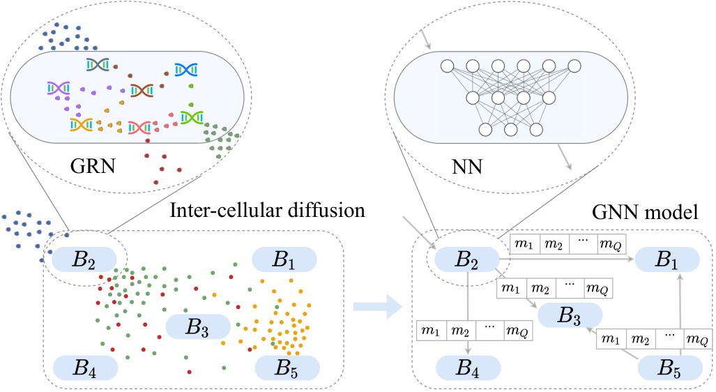
Bacterial cells are equipped with various regulatory systems, such as single/two/multi-component systems including Quorum sensing (QS), to respond to environmental stimuli. The receptors and transporters on cell membranes can react and transport extracellular molecules, which subsequently interact with respective genes. In turn, the GRN is triggered to go through a complex non-linear computational process in response to the input signals. In the literature, it has been suggested that the computational process through the GRN of a bacterial cell comprises a hidden neural network (NN)-like architecture [6, 7]. This indicates that, even though bacterial cells can be categorized as non-neural organisms, they perform neural decision-making processes through the GRN. This results in recent attention towards Molecular Machine Learning systems, where AI and ML are developed using molecular systems[8]. In these systems, several neural components can be identified in GRNs, in which genes may be regarded as computational units or neurons, transcription regulatory factors as weights/biases and proteins/second messenger Molecular Communications (MC) as neuron-to-neuron interactions. Owing to a large number of genes and the interactions in a GRN, it is possible to infer sub-networks with NN behaviors that we term Gene Regulatory Neural Networks (GRNN). The non-linear computing of genes results from various factors that expand through multi-omics layers, including proteomic, transcriptomic and metabolomic data (further explained in Section II-A). In contrast, the GRNN is a pure NN of genes with summarized non-linearity stemmed from multi-omics layers with weights/biases.
Identification of GRNNs can be used to model the decision-making process of the cell precisely, especially considering simultaneous multiple MC inputs or outputs. However, due to the limited understanding and data availability, it is still impossible to model the complete GRN with its NN-like behaviors. Therefore, this study uses a GRNN of Pseudomonas aeruginosa that is associated with PhoR-PhoB and BqsS-BqsR two-component systems (TCSs) and three QS systems related to pyocyanin production as a use case to explore the NN-like behaviors. Although a single bacterium can do a massive amount of computing, they prefer living in biofilms. Hence, in order to understand the biofilm decision-making mechanism, we extend this single-cell computational model to an ecosystem level by designing an in-silico single species biofilm with inter-cellular MC signaling as shown in Fig. 1.
The contributions of this study are as follows:
- •
Extracting a GRNN: Due to the complexity and insufficient understanding of the gene expression dynamics of the full GRN, we only focus on a sub-network associated with pyocyanin production (shown in Fig. ) to investigate the NN-like computational behavior of the GRN. Further, the genes of extracted sub-network are arranged following a NN structure that comprises input, hidden and output layers, as shown in Fig. .
- •
Modeling a biofilm as a GNN: The GRNN only represents the single-cell activities. To model the biofilm-wide decision-making process, we use a Graph Neural Network (GNN). First, we create a graph network of the bacterial cell and convert it to a GNN by embedding each node with the extracted GRNN as the update function. Second, the diffusion-based MCs between bacterial cells in the biofilm are encoded as the message-passing protocol of the GNN, as shown in Fig. .
- •
Exploring the behaviors of the GRNN and intra-cellular MC dynamics to predict cell decisions: The output of the GRNN is evaluated by comparing it with the transcriptomic and pyocyanin production data from the literature. Finally, an edge-level analysis of the GRNN is conducted to explore the causal relationships between gene expression and pyocyanin production.
This paper is organized as follows: Section II explains the background of bacterial decision-making in two levels: cellular-level in Section II-A and population-level in Section II-B, while the background on the P. aeruginosa is introduced in Section II-C. Section III is dedicated to explaining the model design of cellular and population levels. The results related to model validation and the intergenic intra-cellular signaling pattern analysis are presented in Section IV and the study is concluded in Section V.
II Background
As the model expands through single cellular and biofilm-wide decision-making layers, this section provides the background of how a bacterium uses the GRN to make decisions and how bacterial cells make decisions in biofilms. Moreover, we briefly discuss the cellular activities of the Pseudomonas aeruginosa as it is the use case species of this study.
II-A Decision-Making Process of an Individual Cell
Prokaryotic cells are capable of sensing the environment through multiple mechanisms, including TCSs that have been widely studied and it is one of the focal points of this study. The concentrations of molecular-input signals from the extracellular environment influence the bacterial activities at the cellular and ecosystem levels [9]. Apart from the extracellular signals of nutrients, it is evident that the QS input signals have a diverse set of regulative mechanisms in biofilm-wide characteristics, including size and shape [10]. These input signals undergo a computational process through the GRN, exhibiting a complex decision-making mechanism. Past studies have explored and suggested this underpinning computational mechanism in a plethora of directions, such as using differential equations [11] and probabilistic Boolean networks [12] and logic circuit [13]. All of these models mainly infer that the bacterial cells can make decisions not just based on the single input-output combinations, but they can integrate several incoming signals non-linearly to produce outputs.
The studies that focus on differences in gene expression levels suggest that a hidden weight behavior controls the impact of one gene on another [6]. This weight behavior emerges through several elements, such as the number of transcription factors that induce the expression, the affinity of the transcription factor binding site, and machinery such as thermoregulators and enhancers/silencers [14, 15]. Fig. 3 depicts a set of factors influencing the weight between genes. The weight of an edge between two genes has a higher dynamicity as it is combinedly determined by several of these factors.
Based on environmental conditions, the GRN of the bacterial cell adapts various weights to increase the survivability and repress unnecessary cellular functions to preserve energy. An example of such regulation is shown in Fig. 4 where a P. aeruginosa cell uses a thermoregulator to regulate the QS behaviors. Fig. has a set of relative weights based on cellar activities in an environment at 37C, while Fig. represents weights at 30C. The weights between the hn21 and rhlR are different in two conditions, and these cellar activities are further explained in [14].
II-B Biofilm Decision-Making
Even though an individual cell is capable of sensing, computing, and actuating, the majority of bacterial cells live in biofilms, where the survivability is significantly increased compared to their planktonic state. Biofilm formation can cause biofouling and corrosion in water supply and industrial systems [16]. However, biofilms formation can be desirable in many situations, for example, bioreactors in wastewater treatment [17], bioremediation of contaminated groundwater [18, 19], where biofilms serve as platforms for biogeochemical reactions. A massive number of factors can influence biofilm formation, including substratum surface geometrical characteristics, diversity of species constituting the biofilm, hydrodynamic conditions, nutrient availability, and especially communication patterns [20] where the TCS and QS play significant roles. A TCS comprises a histidine kinase that is the sensor for specific stimulus and a cognate response regulator that initiates expressions of a set of genes [21]. Hence, in each stage, essential functions can be traced back to their gene expression upon a response to the input signals detected by bacterial cells. For instance, in the first stage of biofilm formation, the attachment of bacteria to a surface is associated with sensing a suitable surface and altering the activities of the flagella. In the next stage, rhamnolipids production is associated with ferric iron availability in the environment, mostly sensed through BqsS-BqsR TCSs. Further, was identified as a regulator of pqsA, pqsR, and pqsE gene expressions that are associated with the production of two critical components for the formation of microcolonies: eDNA and EPS[22]. Similarly, in the final stage, the dispersion process can also be traced back to a specific set of gene regulations, including bdlA an rbdA [23, 24]. An understanding of the underlying decision-making process of bacteria may enable us to control their cellular activities.


II-C Pseudomonas Aeruginosa
The main reason for selecting P. aeruginosa in this work lies in its alarming role in human health. For example, this species is the main cause of death in cystic fibrosis patients [25]. P. aeruginosa is a gram-negative opportunistic pathogen with a range of virulence factors, including pyocyanin and cytotoxin secretion[26]. These secreted molecules can lead to complications such as respiratory tract ciliary dysfunction and induce proinflammatory and oxidative effects damaging the host cells [27]. The biofilms are being formed on more than 90% endotracheal tubes implanted in patients who are getting assisted ventilation, causing upper respiratory tract infections [28]. In addition, another important reason for targeting P. aeruginosa is the data availability for the GRN structure [29], pathways [30], genome [31], transcriptome [32] and data from mutagenesis studies [33, 34]. Compared to the complexity of the GRN, the amount of data and information available on the gene-to-gene interactions and expression patterns is insufficient to develop an accurate full in-silico model. Therefore, we chose a set of specific genes that are associated with QS, TCS, and pyocyanin production.
III System design
This section explains the system design in two main phases, extracting a NN-like architecture from the GRN targeting the set of genes and creating a model of the biofilm ecosystem.
III-A Extracting Natural Neural Network from GRN
We first fetch the structure of the GRN graph from RegulomePA [29] database that contains only the existence of interactions and their types (positive or negative). As the next step, using information from the past studies [35, 36, 37, 38], we identified the genes involved in the Las, Rhl and PQS QS systems, PhoR-PhoB and BqsS-BqsR TCSs, and pyocyanin production to derive the sub-network of GRN as shown in Fig . We further explored the expression dynamics using transcriptomic data [39, 40] where we observed the non-linearity in computations that are difficult to capture with existing approaches such as logic circuits, etc. [6], making the NN approach more suitable. However, a NN model with a black box that is trained on a large amount of transcriptomic data records to do computations similar to the GRN has a number of limitations, especially in understanding the core of the computational process[41]. Our model does not use a conventional NN model; instead, we extract a NN from the interaction patterns of the GRN, which we consider a pre-trained GRNN. In this sub-network, we observed that the lengths of expression pathways are not equal. For example, the path from PhoR-PhoB to the phz2 gene has two hops, but the path from the BqsS-BqsR system to the rhlR gene only has one hop. The extracted network has the structure of a random NN. Hence, we transform this GRNN to Gene Regulatory Feedforward Neural Network by introducing hypothetical nodes (hns) that do not affect the behaviors of the GRNN as shown in Fig . In this transformation, we decide the number of hidden layers based on the maximum number of hops in gene expression pathways. In our network, the maximum number of hops is two, which determines the number of hidden layers as one, and then the number of hops of all the pathways is leveled by introducing hns. If a hn is introduced between a source and target genes, the edge weights from the source node to the hn and from hn to the target node are made “1” so that the hn does not have an influence on the regulation of genes. Moreover, if a gene does not induce another in the network, the weight of the edge between that pair is made “0”.
Here, we summarize multiple factors of interaction into a weight that determines the transcriptional regulation of a particular gene. This regulation process occurs when the gene products get bound to the promoter region of another, influencing the transcriptional machinery. Hence, we observe this regulation process of a target gene as a multi-layered model that relies on the products of a set of source genes, the interaction between gene products, and the diffusion dynamics within the cell. Creating a framework to infer an absolute weight value using all the above factors is a highly complex task. In order to infer weight, one method is to train a NN model with the same structure as the GRN using a series of transcriptomic data. However, this approach also has numerous challenges, such as the lack of a sufficient amount of data in similar environments.
Therefore, we estimate a set of relative weights based on genomic, transcriptomic, and proteomic explanations of each interaction from the literature. The weights were further fine-tuned using the transcriptomics data. A relative weight value of an edge can be considered a summarizing of multi-layer transcriptional-translation to represent the impact of the source gene on a target gene.
In this computational process, we identify another layer of interactions that occur within the cell. The produced molecules by the considered TCs network go through a set of metabolic interactions that are crucial for the functionality of the cell. Since our primary goal is to explore the NN behaviors of GRN, we model these inter-cellular chemical reactions as a separate process, keeping the gene-to-gene interactions and metabolic interactions in two different layers. To model the complete pyocyanin production functionality of the cell, we use the inter-cellular molecular interactions shown in Fig 5. Here, RhlR is a transcriptional regulator of P. aeruginosa that forms a complex by getting attached to its cognate inducer C4-HSL and then binds to the promoter regions of relevant genes [42]. Similarly, LasR transcriptional regulator protein and 3-oxo-C12-HSL (3OC), and PqsR with PQS and HHQ form complexes and get involved in the regulation of a range of genes [43, 44]. Further, C10H10O6 in the environment are converted by the P. aeruginosa cells in multiple steps using the products of the GRNN we consider. First, C10H10O6 is converted into phenazine-1-carboxylic using the enzymes of pqsABCDEFG genes. Later, phenazine-1-carboxylic was converted into 5-Methylphenazine-1-carboxylate, and finally, 5-Methylphenazine-1-carboxylate into Pyocyanin by PhzM and PhzS, respectively [45].
Molecular accumulation within a bacterial cell can be considered its memory module where certain intra-cellular interactions occurs. Therefore, we define an internal memory matrix as,
| (1) |
where the concentration of the internal molecule is .
GRNN process molecular signals from the environment and other cells. Hence, we used the approach of GNN as a scalable mechanism to model the MCs and biofilm wide decision-making process. The extreme computational power demand of modeling the diffusion-based MCs of each cell is also avoided by using this approach.
III-B Graph Neural Network Modeling of Biofilm
First, the biofilm is created as a graph network of bacterial cells where each node is a representation of a cell, and an edge between two nodes is a MC channel. We convert the graph network into a Graph Neural Network (GNN) in three steps: 1) embedding the extracted GRNN of pyocyanin production into each node as the update function, 2) encoding the diffusion-based cell-to-cell MC channels as the message passing scheme, and 3) creating an aggregation function at the reception of molecular messages by a node as shown in Fig. 6. Next, we define feature vectors of each node of the GNN to represent the gene expression profile of the individual cell at a given time. Subsequently, considering is the number of genes in the GRNN, is the number of bacterial cells in the biofilm and is the expression of gene by the bacteria , we derive the following matrix that represents all the feature vectors of the GNN at time .
| (2) |
The computational output of the GRNN of each node results in the secretion of a set of molecules that are considered messages in our GNN model as illustrated in the Fig. 7.
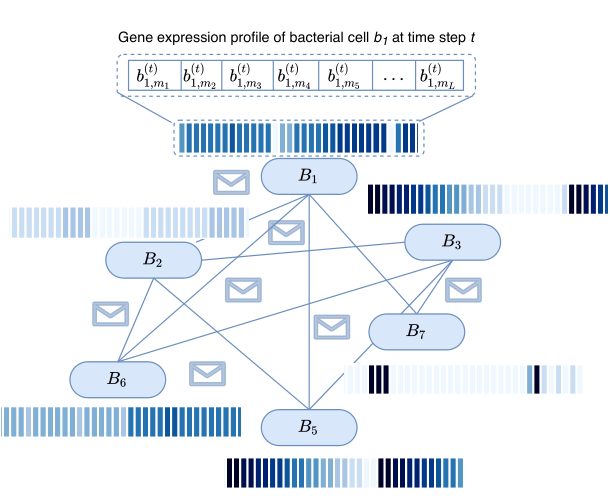
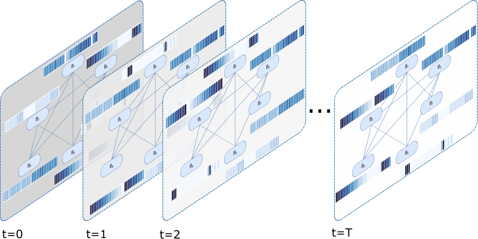

When the number of molecular species considered in the network is and output molecular message from bacterial cell at TS is , we derive the matrix
| (3) |
| Parameter | Value | Description |
|---|---|---|
| No. of cells | 2000 | The number of cells is limited due to the memory availability of the server. |
| No. of genes | 13 | The network only consists of the gene that are directly associated with QS, PhoR-PhoB and BqsS-BqsR TCSs, and pyocyanin production. |
| No. internal memory molecules | 16 | The set of molecules that involved in QS, PhoR-PhoB and BqsS-BqsR TCSs,and pyocyanin production. |
| No. messenger molecules | 4 | The number of molecules that were exchanged between cells in the sub network. |
| Dimensions of the environment | 20x20x20 | The dimensions were fixed considering the average sizes of P. aeruginosa biofilms and computational demand of the model. |
| Duration | 150 TSs | The number of TSs can be modified to explore the cellular and ecosystem level activities. For this experiment we fixed a TS to represent 30mins. |
| No. iterations per setup | 10 | Considering the stochasticity ranging from the gene expression to ecosystem-wide communications, the experiments were iterated 10 times. |
Further, we use a static diffusion coefficients vector
| (4) |
where is diffusion coefficient of molecular species .
We define another matrix that contains the euclidean distances between bacterial cells in the biofilm as follows
| (5) |
where is the euclidean distance between the and cells.
The feature vector of bacterial cell at the TS is then modeled as,
| (6) |
where is the message generated by the same cell in the previous TS. The is the extracted GRNN that is the update function in the GNN learning process and , is the aggregate function. In the aggregation component, the is the incoming signals from peer bacterial cells and is the external molecule input vector at the location of and the TS that is expressed as
| (7) |
In order to compute , we use a matrix ; , where is an all-ones matrix of dimension . The matrix is then defined as follows,
| (8) |
In the above matrix, is the Green’s function of the diffusion equation as shown below,
| (9) |
Further, the incoming signal vector is denoted as below,
| (10) |
Further, we equip our model with a 3-D environment to compensate for the noise element and external molecule inputs. Environment-layer is designed as a 3-D grid of voxels that can store precise information on external nutrients (similarly to our previous model in [46]). The diffusion of nutrient molecules through the medium is modeled as a random-walk process. This layer allows us to enrich the model with the dynamics of nutrient accessibility of bacterial cells due to diffusion variations between the medium and the Extracellular Polymeric Substance (EPS).
The bacterial cells in the ecosystem also perform their own computing tasks individually, resulting in a massively parallel processing framework. Hence, we use the python-cuda platform to make our model closer to the parallel processing architecture of the biofilm, where we dedicate a GPU block for each bacterial cell and the threads of each block for the matrix multiplication of the GRNN computation associated with the particular cell. Additionally, due to the massive number of iterative components in the model, the computational power demand faces significant challenges with serial programming making parallelization the best match for the model.
IV Simulations
In this section, we first explain the simulation setup and then discuss the results of gene expression and molecular production dynamics to prove the accuracy of the extracted GRNN, emphasizing that it works similarly to the real GRN. Later, we use computing through the GRNN to explain certain activities of the biofilm.
IV-A Simulation Setup
As our interest is to investigate the NN-like computational process, we do not model the formation process of the biofilm, but we only remodel a completely formed biofilm and disregarding the maturation and dispersion stages. In this model, we consider the biofilm as a static 3-D structure of bacterial cells. Hence, we first place bacterial cells randomly in the model in a paraboloid shape using the equation, where , and are the components of 3-D Cartesian coordinates. This paraboloid shape is chosen to make the spacial arrangement of the cells close to real biofilm while keeping the cell placement process mathematically simple. Within this 3-D biofilm region, we model the diffusivity according to , which is the mean relative diffusion [47] where and are the average molecular diffusion coefficients of the biofilm and pure water, respectively. Further, to start the simulation at a stage where the biofilm is fully formed and the MC is already taking place, we filled the internal memory vector of each cell with the average molecular level at the initial TS. Each bacterial cell will use the initial signals from the internal memory and use its GRNN to process and update the feature vector for the next TS. Table I presents the parameter descriptions and values used for the simulation. As shown in Table I, the model runs for 150 TSs, generating data on a range of functions for the system. For instance, this model can produce data on feature vector of each cell, MC between cells, molecular consumption by cells, secretion to the environment, and nutrient accessibility of cells for each TS.


In order to prove that our GRNN computes similarly to the natural bacterial cell and collective behaviors of the cells are the same as the natural biofilm, we conduct a series of experiments. We explore the GRNN computation and biofilm activities under High Phosphate (HP) and Low Phosphate (LP) levels using eight experimental setups as follows, 1) wild-type bacteria (WD) in LP, 2) lasR mutant (lasR) in LP, 3) phoB mutant (phoB) in LP, 4) lasR & PhoB double mutant (LasRPhoB) in LP, 5) WD in HP, 6) lasR in HP, 7) PhoB in HP and LasRPhoB in HP. While the WD uses the full GRNN, lasR is created by making the weight of the link between hn22 and lasR as “0”. Further, the GRNN of phoB is created by making the weights of links from PhoB to hn23 and PhoB to pqsABCDE also “0”.
IV-B Model Validation

First, we show the nutrient accessibility variation in the biofilm through Fig 8. The cells in the biofilm core have less accessibility while the cells closer to the periphery have more access to nutrients due to variations in diffusion between the environment and the EPS. Fig shows that when a low phosphate concentration is introduced to the environment, the direct access to the nutrient by the cells is limited. After the , around 60% of cells have access to 20% of the nutrient concentration. Further, Fig shows that the increased nutrient introduction to the environment positively reflects on the accessibility. This accessibility plays a role mainly in the deviation of gene expression patterns resulting in phenotypic differentiations that is further analyzed in Section IV-C.


Comparing the predictions of molecular production through GRNN computing with the wet-lab experimental data from the literature, we are able to prove that the components of the GRN work similarly to a NN. Fig. 9 shows the pyocyanin accumulation variations of the environment in the eight setups mentioned earlier as results of decision-making of the GRNN. Production of pyocyanin of the WD P. aeruginosa biofilms is high in LP, compared to the HP environments as shown in Fig: . Further, the same pattern can be observed in the lasR biofilms, but with a significantly increased pyocyanin production in LP as shown in Fig. . The phob and LasRphob biofilms produce a reduced level of pyocyanin compared to WD and LasR that are shown in Fig. and Fig. respectively. We then present a comparison between GRNN prediction and wet-lab experimental data [48] as ratios of HP to LP in Fig. 10. The differences between pyocyanin production through GRNN in HP and LP condition for all the four setups in Fig. 10 are fairly close to the wet-lab data. In the WD setup, the difference between the GRNN model and wet-lab data only has around 5% difference, while deviations around 10% can be observed in lasR and phoB. The most significant deviation around 20% of pyocyanin production difference is visible in lasRphoB that is caused by the lack of interaction from other gene expression pathways, as we only extracted a sub-network portion of the GRN. Therefore, these results prove that the extracted GRNN behaves similarly to the GRN dynamics.

We further prove that the GRNN computing process performs similarly to the GRN by comparing the gene expression behaviors of the model with the wet-lab data [48] as shown in Fig. 11. First, we show the expression dynamics of genes lasI, pqsA and rhlR of WD in LP in Fig. , Fig. and Fig. respectively. All the figures depict that gene expression levels are higher in LP compared to HP until around . Beyond that point, relative gene expression levels are close to zero as the the environment run out of nutrients. Moreover, the differences in gene expression levels predicted by the GRNN computing for LP and HP are also compared with the wet-lab data in Fig. . In this comparison, it is evident that the predicted gene expression differences of all three genes are close to the wet-lab data with only around 10% variation. The performance similarities between the GRNN and real cell activities once again prove that the GRN has underpinning NN-like behaviors.
IV-C Analysis of GRNN Computing
Fig. 12 and Fig. 13 are used to show the diverse information flow of the GRNN that cause the variations in pyocyanin production in LP and HP conditions, respectively. Here, we use gene expression profiles extracted from one bacterial cell located at (7, 9, 2)m in the Cartesian coordinates that is in the middle region of the biofilm with limited access to the nutrients. First, the gene expression variations of WD, lasR, and phob bacterial cells in LP (Fig. 12) and HP (Fig. 13) are shown for . Next, the information flow through the GRNN is illustrated above each expression profile at time , where the variations will be discussed. In Fig. , impact of the inputs 3OC-LasR and phosphate cause higher expression levels of the nodes hn12 and phoB in the input layer that cascade the nodes phZ1, phZ2, pqsR, lasR, 3OC, rhlR and PqsH in the output layer at . Fig. has significantly higher pqsA operon expression levels compared to HP conditions (Fig. ), reflecting higher pyocyanin production that can be seen in Fig. . Nevertheless, the reduced gene expression levels, except pqsA operon, of lasR biofilm in both LP (Fig. ) and HP (Fig. ) conditions compared to the other setups emphasize that the inputs via inter-cellular MC significantly alter GRNN computing outputs. In contrast, only a smaller gene expression difference can be observed between the two setups of phob in LP (Fig. and phob in HP (Fig. ) resulting in minimized pyocyanin production differences as shown earlier in Fig. .
The GRNN model supports the understanding of the gene expression variations due to factors such as nutrient accessibility, where in our case is a single species biofilm. Fig. 14 depicts the variability in the gene expression levels for four different locations of the biofilm at . Fig. 14a and Fig. 14b are the gene expression profiles and the signal flow through GRNN pairs of two cells located close to the attached surface and the center of the biofilm. The phosphate accessibility for these two locations is limited. Hence, edges from phob have a higher information flow compared to the other two cells near the periphery of the biofilm, which can be observed in Fig. 14c and Fig. 14d. The microbes in the center (Fig. 14a) and the bottom (Fig. 14b) mainly have access to the inter-cellular MCs, while the other two bacteria have direct access to the extracellular phosphate.
This GRNN produced data can further be used to understand the spatial and temporal dynamics of phenotypic clustering of gene expressions which is important in predicting and diagnosis of diseases[49]. Fig. 15 shows the phenotypic variation of WD biofilm in LP. Fig. 15a shows the number of cluster variations over the first 30 when the significant phenotypic changes of the biofilm is evident. At around and , the bacterial cells have the most diverse expression patterns due to the highest extracellular nutrient penetration (can be seen in Fig. ) to the biofilm and inter-cellular communications. Here we use four TSs ( - Fig. 15b, - Fig. 15c, - Fig. 15d and - Fig. 15e) to analyze this phenotypic differentiation. Each pair of Uniform Manifold Approximation and Projection (UMAP) plot and diagram of cell locations of each cluster explain how nutrient accessibility contribute to the phenotypic clustering. Although at (Fig. 15) the average number of clusters is over four, there are only two major clusters that can be observed with higher proportions, as shown in the pie chart. Among the two major clusters (blue and green) of Fig. 15b, the bacteria in the blue cluster can mostly be found in the center of the biofilm, while the green cluster cells are close to the periphery. Fig. 15c and Fig. 15d have more clusters as the nutrient accessibility among cells is high. In contrast, due to the lack of nutrients in the biofilm, a limited number of clusters can be seen in the biofilm after around , which can be observed Fig. 15e.
V Conclusion
The past literature has captured the non-linear signal computing mechanisms of Bacterial GRNs, suggesting underpinning NN behaviors. This study extracts a GRNN with summarized multi-omics gene expression regulation mechanisms as weights that can further analyze gene expression dynamics, design predictive models, or even conduct in-vivo computational tasks. We used P. aeruginosa single species biofilm as a use case and extracted relevant gene expression data from databases such as RegulomePA and transcriptomic data from databases including GEO. Due to the complexity of the GRN and expression dynamics, we only considered a smaller sub-network of the GRN as a GRNN that is associated with QS, iron and phosphate inputs, and pyocyanin production. Considering this GRNN, we modeled the computation process that drives cellular decision-making mechanism. As bacteria live in ecosystems in general where intra-cellular communication play a significant role in cellular activities, an in-silico biofilm is modeled using GNN to further analyze the biofilm-wide decision-making. A comparison between the GRNN generated data and the transcriptomic data from the literature exhibits that the GRN behaves similarly to a NN. Hence, this model can explore the causal relationships between gene regulation and cellular activities, predict the future behaviors of the biofilm as well as conduct bio-hybrid computing tasks. Further, in the GRNN extraction phase, we were able to identify the possibility of modeling more network structures with various number of input nodes, hidden layers, and output nodes. In addition, GRN components including auto regulated genes and bidirectional intergenic interactions hints the possibility of extracting more sophisticated types of GRNNs such as Recurrent NN and Residual NN in the future. The idea of extracting sub-networks as NNs can lead to more intriguing intra-cellular distributed computing. Further, this model can be extended to multi-species ecosystems for more advanced predictive models as well as distributed computing architectures combining various NNs.
References
- [1] E. Alm, K. Huang, and A. Arkin, “The evolution of two-component systems in bacteria reveals different strategies for niche adaptation,” PLoS Computational Biology, vol. 2, no. 11, p. e143, 2006.
- [2] D. F. Blair, “HOW BACTERIA SENSE AND SWIM,” Annual Review of Microbiology, vol. 49, pp. 489–520, Oct. 1995.
- [3] C. Wang, S. Xu, and Z.-P. Liu, “Evaluating gene regulatory network activity from dynamic expression data by regularized constraint programming,” IEEE Journal of Biomedical and Health Informatics, vol. 26, no. 11, pp. 5738–5749, 2022.
- [4] M. Land, L. Hauser, S.-R. Jun, I. Nookaew, M. R. Leuze, T.-H. Ahn, T. Karpinets, O. Lund, G. Kora, T. Wassenaar, S. Poudel, and D. W. Ussery, “Insights from 20 years of bacterial genome sequencing,” Functional & Integrative Genomics, vol. 15, pp. 141–161, Feb. 2015.
- [5] D. Ravì, C. Wong, F. Deligianni, M. Berthelot, J. Andreu-Perez, B. Lo, and G.-Z. Yang, “Deep learning for health informatics,” IEEE journal of biomedical and health informatics, vol. 21, no. 1, pp. 4–21, 2016.
- [6] J. VOHRADSKY, “Neural network model of gene expression,” the FASEB journal, vol. 15, no. 3, pp. 846–854, 2001.
- [7] D. C. Weaver, C. T. Workman, and G. D. Stormo, “Modeling regulatory networks with weight matrices,” in Biocomputing’99, pp. 112–123, World Scientific, 1999.
- [8] S. Balasubramaniam, S. Somathilaka, S. Sun, A. Ratwatte, and M. Pierobon, “Realizing molecular machine learning through communications for biological ai: Future directions and challenges,” arXiv preprint arXiv:2212.11910, 2022.
- [9] B. D. Unluturk, S. Balasubramaniam, and I. F. Akyildiz, “The impact of social behavior on the attenuation and delay of bacterial nanonetworks,” IEEE transactions on nanobioscience, vol. 15, no. 8, pp. 959–969, 2016.
- [10] T. De Kievit, “Quorum sensing in pseudomonas aeruginosa biofilms,” Environmental microbiology, vol. 11, no. 2, pp. 279–288, 2009.
- [11] T. Chen, H. L. He, and G. M. Church, “Modeling gene expression with differential equations,” in Biocomputing’99, World Scientific, 1999.
- [12] I. Shmulevich, E. Dougherty, and W. Zhang, “From boolean to probabilistic boolean networks as models of genetic regulatory networks,” Proceedings of the IEEE, vol. 90, no. 11, pp. 1778–1792, 2002.
- [13] D. Wang, K.-K. Yan, C. Sisu, C. Cheng, J. Rozowsky, W. Meyerson, and M. B. Gerstein, “Loregic: a method to characterize the cooperative logic of regulatory factors,” PLoS computational biology, vol. 11, no. 4, p. e1004132, 2015.
- [14] M. V. Grosso-Becerra, G. Croda-García, E. Merino, L. Servín-González, R. Mojica-Espinosa, and G. Soberón-Chávez, “Regulation of pseudomonas aeruginosa virulence factors by two novel rna thermometers,” Proceedings of the National Academy of Sciences, vol. 111, no. 43, pp. 15562–15567, 2014.
- [15] A. Ishihama, “Prokaryotic genome regulation: a revolutionary paradigm,” Proceedings of the Japan Academy, Series B, vol. 88, no. 9, pp. 485–508, 2012.
- [16] M. Fletcher, “Bacterial biofilms and biofouling,” Current opinion in biotechnology, vol. 5, no. 3, pp. 302–306, 1994.
- [17] N. Qureshi, B. A. Annous, T. C. Ezeji, P. Karcher, and I. S. Maddox, “Biofilm reactors for industrial bioconversion processes: employing potential of enhanced reaction rates,” Microbial cell factories, vol. 4, no. 1, pp. 1–21, 2005.
- [18] C. Kao, S. Chen, and J. Liu, “Development of a biobarrier for the remediation of pce-contaminated aquifer,” Chemosphere, vol. 43, no. 8, pp. 1071–1078, 2001.
- [19] D. P. Martins, K. Leetanasaksakul, M. T. Barros, A. Thamchaipenet, W. Donnelly, and S. Balasubramaniam, “Molecular communications pulse-based jamming model for bacterial biofilm suppression,” IEEE Transactions on NanoBioscience, vol. 17, no. 4, pp. 533–542, 2018.
- [20] C. C. Goller and T. Romeo, “Environmental influences on biofilm development,” in Current Topics in Microbiology and Immunology, pp. 37–66, Springer Berlin Heidelberg, 2008.
- [21] T. Mascher, J. D. Helmann, and G. Unden, “Stimulus perception in bacterial signal-transducing histidine kinases,” Microbiology and molecular biology reviews, vol. 70, no. 4, pp. 910–938, 2006.
- [22] D. Passos da Silva, M. C. Schofield, M. R. Parsek, and B. S. Tseng, “An update on the sociomicrobiology of quorum sensing in gram-negative biofilm development,” Pathogens, vol. 6, no. 4, p. 51, 2017.
- [23] M. Toyofuku, T. Inaba, T. Kiyokawa, N. Obana, Y. Yawata, and N. Nomura, “Environmental factors that shape biofilm formation,” Bioscience, biotechnology, and biochemistry, vol. 80, no. 1, pp. 7–12, 2016.
- [24] K. P. Rumbaugh and K. Sauer, “Biofilm dispersion,” Nature Reviews Microbiology, vol. 18, pp. 571–586, June 2020.
- [25] J. A. Driscoll, S. L. Brody, and M. H. Kollef, “The epidemiology, pathogenesis and treatment of pseudomonas aeruginosa infections,” Drugs, vol. 67, no. 3, pp. 351–368, 2007.
- [26] T. Strateva and I. Mitov, “Contribution of an arsenal of virulence factors to pathogenesis of pseudomonas aeruginosa infections,” Annals of Microbiology, vol. 61, pp. 717–732, May 2011.
- [27] G. W. Lau, D. J. Hassett, and B. E. Britigan, “Modulation of lung epithelial functions by pseudomonas aeruginosa,” Trends in microbiology, vol. 13, no. 8, pp. 389–397, 2005.
- [28] E. Pericolini, B. Colombari, G. Ferretti, R. Iseppi, A. Ardizzoni, M. Girardis, A. Sala, S. Peppoloni, and E. Blasi, “Real-time monitoring of pseudomonas aeruginosa biofilm formation on endotracheal tubes in vitro,” BMC Microbiology, vol. 18, Aug. 2018.
- [29] E. Galán-Vásquez, B. C. Luna-Olivera, M. Ramírez-Ibáñez, and A. Martínez-Antonio, “RegulomePA:a database of transcriptional regulatory interactions in pseudomonas aeruginosa pao1,” Database, 2020.
- [30] R. Caspi, R. Billington, I. M. Keseler, A. Kothari, M. Krummenacker, P. E. Midford, W. K. Ong, S. Paley, P. Subhraveti, and P. D. Karp, “The MetaCyc database of metabolic pathways and enzymes - a 2019 update,” Nucleic Acids Research, vol. 48, pp. D445–D453, Oct. 2019.
- [31] G. L. Winsor, E. J. Griffiths, R. Lo, B. K. Dhillon, J. A. Shay, and F. S. L. Brinkman, “Enhanced annotations and features for comparing thousands of pseudomonas genomes in the pseudomonas genome database,” Nucleic Acids Research, vol. 44, pp. D646–D653, Nov. 2015.
- [32] T. Barrett, S. E. Wilhite, P. Ledoux, C. Evangelista, I. F. Kim, M. Tomashevsky, K. A. Marshall, K. H. Phillippy, P. M. Sherman, M. Holko, A. Yefanov, H. Lee, N. Zhang, C. L. Robertson, N. Serova, S. Davis, and A. Soboleva, “NCBI GEO: archive for functional genomics data sets—update,” Nucleic Acids Research, vol. 41, Nov. 2012.
- [33] H. D. Kulasekara, I. Ventre, B. R. Kulasekara, A. Lazdunski, A. Filloux, and S. Lory, “A novel two-component system controls the expression of pseudomonas aeruginosa fimbrial cup genes,” Molecular Microbiology, vol. 55, pp. 368–380, Nov. 2004.
- [34] S. L. N. Kilmury and L. L. Burrows, “The pseudomonas aeruginosa PilSR two-component system regulates both twitching and swimming motilities,” mBio, vol. 9, Sept. 2018.
- [35] V. Venturi, “Regulation of quorum sensing in pseudomonas,” FEMS microbiology reviews, vol. 30, no. 2, pp. 274–291, 2006.
- [36] V. I. Francis, E. C. Stevenson, and S. L. Porter, “Two-component systems required for virulence in pseudomonas aeruginosa,” FEMS microbiology letters, vol. 364, no. 11, 2017.
- [37] M. Sultan, R. Arya, and K. K. Kim, “Roles of two-component systems in pseudomonas aeruginosa virulence,” International Journal of Molecular Sciences, vol. 22, no. 22, p. 12152, 2021.
- [38] G. Chambonnier, L. Roux, D. Redelberger, F. Fadel, A. Filloux, M. Sivaneson, S. De Bentzmann, and C. Bordi, “The hybrid histidine kinase lads forms a multicomponent signal transduction system with the gacs/gaca two-component system in pseudomonas aeruginosa,” PLoS genetics, vol. 12, no. 5, p. e1006032, 2016.
- [39] N. N. Kreamer, J. C. Wilks, J. J. Marlow, M. L. Coleman, and D. K. Newman, “Bqsr/bqss constitute a two-component system that senses extracellular fe (ii) in pseudomonas aeruginosa,” Journal of bacteriology, vol. 194, no. 5, pp. 1195–1204, 2012.
- [40] H. Huang, X. Shao, Y. Xie, T. Wang, Y. Zhang, X. Wang, and X. Deng, “An integrated genomic regulatory network of virulence-related transcriptional factors in pseudomonas aeruginosa,” Nature communications, vol. 10, no. 1, pp. 1–13, 2019.
- [41] A. Akay and H. Hess, “Deep learning: current and emerging applications in medicine and technology,” IEEE journal of biomedical and health informatics, vol. 23, no. 3, pp. 906–920, 2019.
- [42] J. R. Lamb, H. Patel, T. Montminy, V. E. Wagner, and B. H. Iglewski, “Functionaldomains of the rhlr transcriptional regulator of pseudomonas aeruginosa,” Journal of bacteriology, vol. 185, no. 24, 2003.
- [43] J. P. Pearson, E. C. Pesci, and B. H. Iglewski, “Roles of pseudomonas aeruginosa las and rhl quorum-sensing systems in control of elastase and rhamnolipid biosynthesis genes,” Journal of bacteriology, vol. 179, no. 18, pp. 5756–5767, 1997.
- [44] D. S. Wade, M. W. Calfee, E. R. Rocha, E. A. Ling, E. Engstrom, J. P. Coleman, and E. C. Pesci, “Regulation of pseudomonas quinolone signal synthesis in pseudomonas aeruginosa,” Journal of bacteriology, vol. 187, no. 13, pp. 4372–4380, 2005.
- [45] P. Nadal Jimenez, G. Koch, J. A. Thompson, K. B. Xavier, R. H. Cool, and W. J. Quax, “The multiple signaling systems regulating virulence in pseudomonas aeruginosa,” Microbiology and Molecular Biology Reviews, vol. 76, no. 1, pp. 46–65, 2012.
- [46] S. S. Somathilaka, D. P. Martins, W. Barton, O. O’Sullivan, P. D. Cotter, and S. Balasubramaniam, “A graph-based molecular communications model analysis of the human gut bacteriome,” IEEE Journal of Biomedical and Health Informatics, vol. 26, no. 7, pp. 3567–3577, 2022.
- [47] P. S. Stewart, “Diffusion in biofilms,” Journal of Bacteriology, vol. 185, no. 5, pp. 1485–1491, 2003.
- [48] X. Meng, S. D. Ahator, and L.-H. Zhang, “Molecular mechanisms of phosphate stress activation of pseudomonas aeruginosa quorum sensing systems,” MSphere, vol. 5, no. 2, pp. e00119–20, 2020.
- [49] P. Dutta, S. Saha, and S. Gulati, “Graph-based hub gene selection technique using protein interaction information: Application to sample classification,” IEEE journal of biomedical and health informatics, vol. 23, no. 6, pp. 2670–2676, 2019.