Codes and modular curves
Abstract
These lecture notes have been written for a course at the Algebraic Coding Theory (ACT) summer school 2022 that took place in the university of Zurich. The objective of the course propose an in–depth presentation of the proof of one of the most striking results of coding theory: Tsfasman Vlăduţ Zink Theorem, which asserts that for some prime power , there exist sequences of codes over whose asymptotic parameters beat random codes.
Introduction
Algebraic Geometry (AG) codes is a particularly exciting topic lying at the intersection between number theory, algebraic geometry and coding theory. The birth of this research area dates back to the early 80’s with the introduction by Goppa [Gop81] of a new family of codes obtained by evaluating residues of some differential forms on a given curve. Quickly after, Tsfasman, Vlăduţ, Zink [TVZ82] and independently Ihara [Iha81] proved the existence of sequences of modular curves and Shimura curves having an excellent asymptotic ratio number of points v.s. genus. An immediate but extremely striking corollary is the existence of sequences of codes beating the Gilbert Varshamov bound, in short: codes better than random codes. This remarkable and totally unexpected result turned out to be the first stone of the development of a whole theory: that of AG codes. Surprisingly, a very comparable breakthrough happened in graph theory the late 80’s. Indeed, in 1988, Lubotsky, Philips and Sarnak [LPS88] and independently Margulis [Mar88] used Cayley graphs on quotients of to prove the existence of a family of graphs whose girth, i.e. the length of their shortest cycle, exceeds the girth obtained with the probabilistic method. In both situations, coding theory and graph theory, the use of elegant algebraic structures unexpectedly beat random constructions.
The objective of this lecture is to present in an (almost) self-contained presentation, the beginning of this wonderful story: the original proof of Tsfasman, Vlăduţ and Zink Theorem. It should be mentioned that in 1995, Garcia and Stichtenoth [GS95] proposed another and somehow more explicit approach to design sequence of curves (actually function fields but the two objects are equivalent) reaching the so-called Drinfeld–Vlăduţ [VD83]. It could be considered as strange to present the original proof which turns out to be much more complicated than Garcia and Stichtenoth’s one but there are some reasonable motivations for that:
- •
Tsfasman, Vlăduţ and Zink’s proof testifies from the richness of the theory of algebraic geometry codes, with a proof involving deep results from algebraic geometry and number theory.
- •
This original proof is frequently cited while few references give a complete presentation of it and (in my personal opinion), none of the papers of Tsfasman et. al. and Ihara provide an enough detailed proof. In both articles, the proof is made of less than ten lines hiding a huge amount of prerequisites.
- •
Finally, I wished to give that lecture, because this proof is beautiful and elegant and even if I am not among the mathematicians who do maths pour la beauté de la chose11 1 Litterally : “for the beauty of the thing” it is sometimes pleasant to take the time to appreciate the elegance of some development.
Outline of these notes
We start in Section 1 with bases on linear codes and their asymptotic behaviour. Section 2 gives an introduction to algebraic curves by providing the necessary material in algebraic geometry. Section 3 introduces algebraic geometry codes and states the main result: Tsfasman–Vlăduţ–Zink Theorem. The remainder of the notes are dedicated to the proof of this statement. Sections 4 and 5 provide further material on elliptic and modular curves respectively. Section 6 concludes the proof.
Acknowledgements
First, I would like to thank Gianira Alfarano, Karan Khaturia, Alessandro Neri, Violetta Weger, the organisers of the Algebraic Coding Theory Summer School22 2 https://math.uzh.ch/act/ 2022 who gave me the motivation to type-write old hand-written notes. I would probably never have found the time to do it if they did not ask me for. Several colleagues spent time to carefully read these notes. In particular, I express a deep gratitude to Elena Berardini, Maxime Bombar, Grégoire Lecerf, Jade Nardi, Christophe Ritzenthaler, Joachim Rosenthal and Gilles Zémor for their relevant comments on the preliminary version of the notes.
The author is funded by the french Agence nationale de la recherche for the collaborative project ANR-21-CE39-0009-BARRACUDA.
1 Linear Codes
1.1 Context
In the sequel we are interested in linear –ary codes, which are linear subspaces of . What makes the study hard, but also deeply interesting is that we are not only considering elementary objects such as finite dimensional vector spaces but spaces endowed with a metric: the Hamming metric. The Hamming distance between two vectors is denoted by
The Hamming weight of a vector is its Hamming distance to the zero vector.
1.2 Linear codes
Unless otherwise specified, a code will denote a linear subspace . The vectors of are usually referred to as codewords. The dimension of regarded as an –vector space is always denoted by and its minimum distance denoted by is defined as
where the last equality is a consequence of the linearity. The parameters of a code refer to the triple and is usually denoted as , where the cardinality of the base field is recalled in subscript. Finally, one can also be interested in the rate and relative distance of a code, respectively defined and denoted as follows:
A longstanding problem in coding theory is which kind of triples of parameters can be achieved? A code will be considered as “good” if both and are as close as possible to . However, many upper bounds exist, the most elementary one being the Singleton bound saying that for any code with parameters we have
| (1) |
The rationale behind this question is that both and quantify some feature of linear codes. Suppose we are given a transmission channel, that can be either a wire or a wireless communication for instance an exchange between electronic devices like between a computer and a WiFi antenna. The rate is nothing but the ratio of information divided by the quantity of data which is actually sent across the channel. Hence, the rate quantifies the efficiency of encoding.
On the other hand, the minimum distance quantifies how far are words from each other and hence the theoretical ability to recover an original message from a corrupted codeword33 3 Here we do not introduce any consideration about practical algorithms to correct errors.
Finally, suppose that our objective is to correct errors from a given channel. Consider for instance the –ary symmetric channel with parameter which takes as input a vector and outputs the vector where and the ’s are independent random variables over taking value with probability and any other value in with probability . The average weight of our error vector satisfies
However, for small values of , deviations may happen and it is possible that our input vector is corrupted by much more than errors. Therefore, it is relevant to consider large values of for which the law of large numbers will assert us that the weight of the error will be close to its expectation.
This last discussion motivates the search of sequences of codes with parameters where
and
Remark 1.
Usually in the literature, the sequences and are not supposed to converge and ’s are used instead of actual limits.
In this setting, the question of the achievable pairs remains open. Some bounds are known:
- •
Singleton bound immediately entails that ;
- •
A more precise bound called Plotkin bound entails that . See for instance [Cou16, Chap. 4]
- •
A principle that “constructing bad codes from good ones is always possible” permits to prove that give an achievable pair any pair with and is achievable too.
Exercise 2.
Prove this last assertion.
- •
More precisely, it has been proved by Manin [VM84], that the frontier between the subdomain of of achievable pairs and the non achievable ones is the graph of a continuous function . However, if proving the existence and the continuity of this function is not very hard, having an explicit description of it remains a widely open problem. An upper bound for is given by the minimum of all the known upper bounds on the achievable pairs .
- •
On the other hand a famous result on the average behaviour of random codes referred to as the Gilbert--Varshamov bound asserts that for a random code44 4 This can be formalised as follows, consider the set of all codes of length and dimension in . This set is finite, and let be a random variable uniformly distributed over this set. with fixed rate , then for any the probability that the relative distance of satisfies
goes to when goes to infinity. The function is the –ary entropy function defined as
In short, the pair for a random sequence satisfies .
In summary, the unknown function whose graph is the frontier of the domain of achievable pairs is known to be continuous, to be bounded from below by the Gilbert–Varshamov bound and bounded from above by the min of all known upper bounds. For a long time, it has been supposed that Gilbert Varshamov bound was optimal and that somehow, no family of codes could asymptotically beat random codes. A breakthrough is due to Tsfasman, Vlăduţ and Zink [TVZ82] who showed that the asymptotic Gilbert Varshamov bound is not always optimal. More precisely, they proved the following statement.
Theorem 3.
Let where is a prime number. Then for any , there exists a sequence of codes whose length goes to infinity and whose asymptotic parameters satisfy
Remark 4.
Actually, the result holds for any where is prime and .
Remark 5.
Actually, the result on codes is the corollary of a statement on the existence of a sequence of algebraic curves with specific properties (see further Theorem 41). This statement on curves has proved by Tsfasman, Vlăduţ and Zink in [TVZ82] and independently by Ihara in [Iha81]. However, Ihara did not rely this result with coding theory while Tsfasman et. al. did.
It turns out that, as illustrated by Figures 1 and 2, for , such codes beat Gilbert Varshamov bound. These codes, are actually far from being random and are constructed using elegant techniques from number theory and algebraic geometry. The objective of these notes is to outline a proof of this incredible result, which is probably one of the major breakthroughs of coding theory.
2 Algebraic curves
The objective of this section is not to provide an in depth lecture of algebraic geometry but only to give the minimal prerequisites in algebraic geometry to understand the sequel of these notes. In particular, here most of the proofs will be omitted. I encourage any reader who feels comfortable with algebraic geometry and for whom reading Harsthorne’s book [Har77] is not harder than reading Harry Potter to skip this section for two reasons:
- •
she/he will not learn anything in it;
- •
for a reader who feels comfortable with the language of schemes, the contents of this section could appear to be dirty.
If you wish further details on algebraic geometry, I can encourage the following readings depending from your knowledge on the topic:
- •
Walker’s book [Wal00] is an excellent first reading if you do not know anything about algebraic geometry and algebraic geometry codes.
- •
If you do not like geometry, Stichtenoth’s book [Sti09] proposes an excellent introduction to algebraic geometry codes from a purely arithmetic point of view. It provides in particular a different proof of the Tsfasman–Vlăduţ–Zink theorem based on so–called recursive towers of function fields which excludes any geometric consideration.
- •
- •
2.1 Plane curves and functions
Let be a perfect field55 5 In the sequel the fields of interest will be either or finite fields . and be its algebraic closure. We denote by and respectively the affine and projective planes over . An affine plane curve over is the vanishing locus in of a nonzero two variables polynomial . Similarly, a projective plane curve is the vanishing locus in of a nonzero homogeneous polynomial . Recall that the projective plane is the set of vectorial lines of or equivalently is the quotient set
and its elements are represented as triples with the equivalence relation if there exists such that , and .
Such an affine (resp. projective) curve is said to be irreducible if (resp. ) is an irreducible polynomial in (resp. ) and absolutely irreducible if (resp. ) is irreducible when regarded as an element of (resp. ).
Example 6.
Suppose and consider the affine curve with equation . This curve is irreducible but not absolutely irreducible. Indeed, over , the equation of the curve factorizes as and this factorisation is not defined over : the polynomial is irreducible over but not over . Geometrically speaking, is the union of the two lines with respective equations and . These lines are not defined over but their union is.
Given an affine irreducible plane curve , the quotient ring is integral and its field of fractions is well–defined and referred to as the function field of . In the projective setting, the function field can also be defined as the field of fractions where are homogeneous polynomials of the same degree with is not divisible by and with the relation:
For an affine curve , elements of can be understood as restrictions of polynomial functions to the curve . Indeed, considering two polynomials regarded as functions , one can consider their restrictions to and a well–known result usually called Hilbert’s Nullstellensatz (see for instance [Ful89, § 1.7]) asserts that their restrictions to are the same if and only if divides and hence if and only if they are congruent modulo the ideal spanned by .
In the projective setting, a homogeneous polynomial cannot be interpreted as a function since an element of is described by a triple but also by any other triple for any . Hence, given a non constant homogeneous polynomial of degree , the evaluation cannot make sense since . Note however that, for such a polynomial, vanishing at a point is a well–defined notion. Moreover, the evaluation of a fraction of two homogeneous polynomials with the same degree makes sense since
This is the reason why we introduce these objects as the good definition of functions on a projective curve.
Remark 7.
Note that we are juggling with and . Here it is crucial no notice that the curve is defined as a set of points with coordinates in , while functions, should be rational functions with coefficients in . On one hand, the function field is defined over and describes the arithmetic of the curve. On the other hand, when describing a curve as a set of points, considering only the points with coordinates in would be too poor: think for instance about the case where is a finite field, in this situation the set of points with coordinates in is finite and might actually be empty! Then, very different equations may provide the same set of points with coordinates in while the sets of points over will be very different. This explains the rationale behind considering the points with coordinates in .
Remark 8.
Note that when speaking about functions, these objects may not be defined everywhere on the curve and may have some poles somewhere. These objects can be understood as the algebraic geometric counterpart of meromorphic functions in complex analysis.
Remark 9.
It is well–known that the projective plane can be covered by affine planes sometimes called affine charts. Indeed one can embed the affine plane into as:
The images of these three embeddings cover the full projective plane. Hence, given a projective curve, one can consider the restriction of the curve on the image of one of the above embeddings and get an affine curve. Practically, starting with a projective curve with equation one can consider for instance the affine curve with equation but also those with equations or . Hence, one can deduce affine curves (affine charts) from a given projective curve. On the other hand, starting from an affine curve with equation the homogeneous polynomial of degree such that (such a homogeneization is unique, details are left to the reader) is the equation of a curve sometimes referred to as the projective closure of .
A crucial fact is that a curve and its projective closure share a common object : their function field remains the very same one.
2.2 Points
A point of is an element (resp. ) such that (resp. ). A point is said to be a rational point or a –point if its coordinates all lie in . More generally, given an extension , one can define the notions of –points of . The set of –points or –points of respectively denoted by and . One of topics of interest for us in the sequel is the case . In this situation, one sees easily that is finite. Indeed, it is a subset of or which are both finite sets. On the other hand has been defined as a set of –points that we sometimes call the geometric points in the sequel, hence we can also denote it as when we wish to emphasize that we are interested in any possible point.
Given an affine (resp. projective) curve defined by the equation (resp. ) over a field , a point with coordinates (resp. ) is said to be singular if
resp.
A non singular point is said to be regular. A curve without singular points is said to be regular or smooth. On the other hand a curve having at least one singular point is said to be singular. It can be proved that the set of singular points of a curve is always finite.
From now on, unless otherwise specified, any curve is smooth projective and absolutely irreducible.
2.3 Galois action on points
Recall that, for the sake of simplicity, we restrict the definitions to the case where the base field is perfect. This is not a strong restriction for the subsequent purpose where will always be either finite or of characteristic zero.
Given a curve defined over , any point has coordinates (or in the projective setting). These coordinates being in while is defined by polynomial equations with coefficients in , there is a natural action of on points of . Note that the coordinates of are algebraic over and hence generate a finite extension of usually denoted . Therefore, even if may be a complicated object (a profinite group), is stabilized by and hence the orbit of is a finite set which is nothing but the orbit of under the action of the finite group , where is the Galois closure of over .
Definition 10.
Let be a perfect field, a closed point of a curve defined over is the orbit of a geometric point under the action of the absolute Galois group .
The number of elements in such an orbit is referred to as the degree of the closed point. It is also the extension degree . A rational point is always closed since it is fixed by any element of the absolute Galois group and hence it equals to its own orbit under this group action.
Remark 11.
If you prefer the language of number theory, closed points are nothing but the geometric analogue of the places of the function field .
Example 12.
Consider the case and the affine curve with equation (a circle). The point with coordinates is a rational point of , i.e. an element of . The complex point , (where ), is a geometric point of , i.e. an element of . Finally, is a closed point of degree of .
2.4 Maps between curves
As usually in algebra, once structures have been introduced: for instance groups, rings, modules, etc., one introduces morphisms between these objects. In the case of curves, we are interested in two kinds of maps referred to as morphisms and rational maps. A rational map between two affine (resp. projective) curves contained in (resp. ) is a map:
resp.
where (resp. ) are elements of (and, in the projective setting, at least one of the three functions is nonzero). The dashed arrow is here to emphasize the fact that this map is not defined at every point but only on a subset66 6 This subset turns out to be dense for a suitable topology called Zariski topology. For affine curves, at any point where have no pole, the map is defined and said to be regular. For projective curves, at any point where for some , have no pole at and are not simultaneously vanishing, the map is well–defined and said to be regular at . A rational map between two curves is said to be regular if it is regular at any point of .
A rational map induces a field extension the other way around which is defined as follows:
The degree of is defined as the degree of this field extension.
Example 13.
Back to example 12. The map
| (2) |
is a rational map. It is also possible to construct a rational map as
| (3) |
Note that these two maps are not inverses to each other.
Finally, the following statements are well–known. Their proofs are omitted.
Proposition 14.
Let be a rational map between two smooth projective absolutely irreducible curves .
- (i)
if is smooth, then is regular;
- (ii)
if is non constant, then it is surjective.
2.5 Valuations
Recall that a local ring is a ring having a unique maximal ideal. The term local comes precisely from the fact that many such rings may be understood as rings of functions characterized by a local property. For instance, given an affine curve and a rational point with coordinates , the ring defined as the subring of of functions which are regular (i.e. have no pole) at . Namely
One can prove that this ring is a local one whose maximal ideal is the ideal:
When the point is smooth, the ring is known to be a discrete valuation ring, which means that the maximal ideal is principal and that, given a generator of this maximal ideal, for any nonzero element , there exists a non negative integer and an element such that . Such a generator of is called a local parameter (or sometimes a uniformising parameter) at . Moreover, the integer does not depend on the choice of the generator and is referred to as the valuation of at and denoted as . Next, one can easily prove that is nothing but the field of fractions of . Then, any function can be written as , where and the valuation of at will be defined as
In summary, we introduced a map
and this map is known to satisfy the following properties,
- •
, ;
- •
, and equality holds when .
Finally, it should be emphasized that, even if we defined the notion at a rational point, one can actually extend the notion to any geometric point by replacing by , i.e. the field of rational functions on with coefficients in . Therefore, the valuation may be defined at any possible point.
2.6 Divisors
A fundamental object when studying the geometry and arithmetic of a curve is divisors which somehow are the curve/function fields counterpart of fractional ideals in the theory of number fields.
Given a smooth curve over a perfect field , a (geometric) divisor is a formal –linear combination of geometric points of . A divisor is said to be rational if it is globally invariant under the action of . Equivalently, it is a formal sum of closed points of .
Hence a divisor on can be represented as
| (4) |
where the ’s are integers and the ’s are geometric points of . The set is referred to as the support of . The divisor is rational if for any such that are in the same orbit under the action of , then .
Remark 15.
We emphasize that a sum of rational points yields a rational divisor but the converse is false. A rational divisor may be a sum of non rational points. See the subsequent Example 16.
Example 16.
Back to the curve of Example 12 defined over with equation , consider the points and . Then, is a rational divisor on the curve if and only if .
The group of divisors is equipped with a partial order relation denoted and defined as follows. Given two divisors
we say that if
In particular, a divisor is said to be positive if , where denotes the zero divisor.
Given a divisor as in (4), its degree is defined as
Given a function , one can associate its divisor denoted and defined as
| (5) |
Such a divisor is called a principal divisor.
Remark 17.
For such an object to be a divisor, we need to show that the sum (5) is finite, i.e. that the ’s are all zero but a finite number of them. This is actually due to a well–known fact appearing in the next statement whose proof is omitted.
Proposition 18.
A nonzero rational function on a curve has only a finite number of zeroes and poles.
Remark 19.
It is worth noting that a principal divisor is rational. Indeed, one can first note that, since and hence has its coefficients in , then for any geometric point and any then .
The following very classical statement is crucial in the sequel.
Proposition 20.
The degree of principal divisor is always .
We finish this discussion with a statement that we admit and which will be useful later.
Proposition 21.
A principal divisor associated to is zero if and only if is constant.
2.7 Genus and Riemann–Roch Theorem
The most elementary curve one may define is the affine line and its projective closure being the projective line . Regular functions on are nothing but univariate polynomials. Regarding such a polynomial as rational function on , it has a pole at the point “at infinity”, i.e. the points with homogeneous coordinates and one can prove that the valuation at this pole is nothing but .
Therefore, the space of polynomials of degree less than or equal to can be (with enough pedantry) defined as the space of rational functions on which are regular everywhere on an affine chart and with valuation larger than or equal to at the point at infinity. Denoting by this point at infinity, then the space can be regarded as the space of rational functions which are either or such that
As the following definition suggests, Riemann–Roch spaces are generalisations for curves of the spaces .
Definition 22 (Riemann–Roch space).
Let be a smooth projective absolutely irreducible curve over and be a rational divisor on . Then the Riemann–Roch space associated to is defined as
This is a vector space over .
Remark 23.
According to the previous discussion, on , we have .
The following statement summarises some properties of Riemann–Roch spaces.
Proposition 24.
- (i)
A Riemann–Roch space is a vector space over of finite dimension;
- (ii)
For any rational divisor , we have ;
- (iii)
For any rational divisor , we have .
With the above statement at hand, we can introduce a fundamental invariant of a curve: its genus. There are dozens of manners to define this object but none of them is trivial. The one given in these notes is far from being satisfying since it is clearly not intuitive. However, it permits to define the object with a minimal amount of material.
Definition 25 (Genus of a curve).
Let be a smooth projective absolutely irreducible curve. The genus of is defined as
where ranges over all the divisors of .
Remark 26.
Exercise 27.
Prove the statement of Remark 26.
Exercise 28.
Using Definition 25, prove that the genus of the projective line is zero.
Note that the effective computation of the genus is not a simple task. However, for smooth plane curves of degree , there is a closed formula (see [Ful89, Prop. VIII.5]):
This permits in particular to prove that the projective line and smooth conics have genus .
Remark 29.
The notion of genus can actually be defined for singular curves. In this context, two distinct invariants respectively called arithmetic genus and geometric genus can be defined. These two invariants coincide when the curve is smooth.
We conclude this section with Riemann–Roch Theorem, which is a crucial statement in the theory of algebraic curves. This statement is admitted and we refer the reader to Fulton [Ful89] or Stichtenoth’s [Sti09] book for a proof. The first part of the statement is actually a straightforward consequence of the definition we gave for the genus (Definition 25).
Theorem 30 (Riemann–Roch Theorem).
Let be a smooth absolutely irreducible curve of genus over and be a rational divisor on . Then
and equality holds when .
2.8 The Riemann–Hurwitz formula
The last statement that will be useful in the sequel is Riemann–Hurwitz formula which relates the genera of two smooth projective absolutely irreducible curves linked by a non constant rational map . Recall that, according to Proposition 14, such a map is regular and surjective. Denoting by its degree (see § 2.4 for the definition of degree), consider any geometric point . Then one can prove that is a finite subset of and that for any but finitely many of them the cardinality of always equals .
The finite number of points of where this no longer holds are called ramified points. Given , and a local parameter at , the ramification index of is defined as
being an element of . It can be proved that this definition does not depend on the choice of the local parameter at . According to the previous definition, for any point but finitely many of them, we have .
Here we have the material to state Riemann–Hurwitz formula.
Theorem 31 (Riemann–Hurwitz formula (Tame version)).
Let be two smooth projective absolutely irreducible curves over and be a rational map. Suppose that for any , the ramification index is prime to the characteristic of . Then, the genera of are related by the following formula.
Remark 32.
According to the previous discussion, the terms of the sum in the above formula are all zero but a finite number of them.
Remark 33.
The assumption “ramification indexes are prime to the characteristic” can be discarded at the cost of replacing the term by a more complicated one. See [Sti09, Thm. 3.4.13].
This formula is particularly useful since many curves are described by a morphism . Since is known to have genus , the genus of can be deduced from the knowledge of the degree of this map and the ramification indexes.
Example 34.
Consider the map (2) of Example 13 but here we regard the curve as a curve over . One sees that any point has 2 preimages by the map if and only one if . Therefore, there are two ramified points both with ramification index (one can show that the map does not ramify at infinity). Moreover, the map has degree . Then, Riemann–Hurwitz formula yields
Since , we deduce that too.
2.9 What about non plane curves?
A last important fact is that some curves are not plane and may be contained in for . It is actually important in the sequel since we are searching for smooth curves over a finite field with arbitrarily large. Since is finite (and equal to ) such a curve may not be embeddable in and requires a larger dimensional ambient space. So, the question is… what remains true when considering curves in with ? and actually, how are such objects defined?
We define a projective subvariety of as the common vanishing locus of the elements of a homogeneous ideal . If this ideal is prime, then the variety will be said to be irreducible and in this setting, the function field of the variety can be defined in the very same manner as in the plane case. Then, the dimension of the variety can be defined as the transcendence degree of the function field over . A curve will be a variety of dimension . Smoothness can be defined very similarly by requiring a non simultaneous vanishing of all the partial derivatives with respect to the variables. All the other objects, rational maps, valuations, divisors, Riemann–Roch spaces can be defined in the very same manner at the cost of heavier notation. Finally all the previous statements on plane curves actually hold for any curve.
3 Algebraic geometry codes
Now, we have the necessary material to define algebraic geometry (AG) codes. Before, let us recall the definition of Reed–Solomon codes that AG codes generalise.
3.1 Reed–Solomon codes
Definition 35.
Let be distinct elements of . Let , the code is defined as
It is well–known that these codes have parameters and hence reach the Singleton bound (1). However, they are constrained in the sense that the ’s should be distinct and hence the length should be bounded by . Thus, even if these codes have optimal parameters, it is hopeless to use them in order to construct an infinite family of codes over a fixed field whose length goes to infinity. Here, curves enter the game. Note first that Reed–Solomon codes may be defined in a much more pedant manner as follows. Consider the projective line and let be the rational points of with respective homogeneous coordinates . Then, may be defined as
This leads to a natural generalisation to algebraic curves. The interest being the fact that a curve may have more rational points than the projective line and hence replacing by an arbitrary curve may provide the opportunity of getting codes of length larger than .
3.2 Algebraic geometry codes
We give a minimal introduction to algebraic geometry (AG) codes. The reader interested in further references is encouraged to have a look at the surveys [HvLP98, Duu08, CR21] or the books [TVN07, Sti09]. We also refer to [HP95, BH08] for references on the decoding of AG codes.
Definition 36.
Let be a smooth absolutely irreducible curve over . Let be an ordered sequence of distinct rational points of . Let be a rational divisor on whose support avoids the points . Then, the algebraic geometry code is defined as
Once the codes are defined, their parameters can be evaluated using the previously introduced material of algebraic geometry.
Theorem 37.
Let be a smooth absolutely irreducible curve of genus over . let be a tuple of rational points of and be a rational divisor on whose support avoids . Suppose that . Then, the parameters of satisfy
| (6) | |||||
| (7) |
Proof.
Denote by the divisor Consider the map
Its image is trivially . The kernel of this map is the subspace of of functions vanishing at . This subspace is nothing but . By assumption, , is negative and hence, from Proposition 24 (ii), . Thus, is injective and
with equality if . Here, the last inequality together with the equality case are due to Riemann–Roch Theorem (Theorem 30).
Let us comment this last result. It was mentioned in § 1.2 that, from Singleton bound (1), any code satisfies
On the other hand, Theorem 37 asserts that an AG code satisfies
In summary, AG codes are in the worst case at “distance from Singleton bound”. Thus, one can expect good codes for a “not too large” genus . On the other hand, the objective is to construct sequences of codes whose length exceeds and more generally construct families of codes over whose length goes to infinity. Thus, for the length to be large, we look for curves with the largest possible number of rational points.
3.3 The problem of infinite sequence of curves with many points compared to their genus
We expect to get sequences of curves over whose genus grows slowly and number of rational points grows quickly. However, these two objectives are somehow in opposition: to get many rational points, we need a large genus. A well–known result due to Weil asserts that for a smooth absolutely irreducible curve over ,
| (8) |
Thus, we look for a good trade off between the genus and the number of rational points. Now, we have the material to reformulate our coding theoretic problem of producing asymptotically good infinite sequences of codes in terms of the construction of sequences of algebraic curves with specific features. For this, let us consider a sequence of curves with sequence of genera . We suppose that the sequence goes to infinity, hence, according to Weil’s bound (8), the sequence of genera should also go to infinity. Let
| (9) |
For any such curve in the sequence, we fix a rational divisor and the sequence of rational points will be chosen as the full list of rational points, i.e. .
Remark 38.
One could ask whether it is possible to have a rational divisor of any degree whose support avoids while ? The answer is positive, such divisors exist and the constraint that the support of should avoid is actually easy to satisfy. See [CR21, Rem. 15.3.8] for a detailed discussion on this specific question.
Then, the codes have parameters satisfying
Therefore, one can eliminate and get
| (10) |
Set
Then, dividing (10) by and letting go to infinity, we get
where is defined in (9). Therefore, any pair lying on the line of equation is achievable.
Remark 39.
Even if the term has been eliminated, this term is worth in order to chose the point in the line of equation you want to target.
Exercise 40.
Prove that by choosing a relevant sequence of rational divisors on the curves , one can reach any point of the line of equation
3.4 The Ihara constant
Now, we would like to estimate the optimal asymptotic parameters that can be achieved. For that, let us introduce the Ihara constant:
Then, the Tsfasman–Vlăduţ–Zink (TVZ) bound asserts the existence of families of codes whose asymptotic parameters satisfy
This opens the question of the value of . The remainder of these notes consists in outlining a proof of the following statement.
Theorem 41.
For and a prime number, we have
Combining the previous result with the TVZ bound, one ca prove that for , and hence when is the square of a prime and is larger than or equal to , the TVZ bound exceeds the Gilbert Varshamov one, proving that some families of codes from algebraic curves are better than random codes.
Let us conclude with some comments.
- •
- •
The TVZ bound is actually optimal. Indeed, subsequently to the publication of Tsfasman–Vlăduţ–Zink result, in [VD83] Drinfeld and Vlăduţ proved that for any prime power , we always have .
- •
The core of the proof of this wonderful result rests on the use of families of curves called modular curves which parameterise families of algebraic curves called elliptic curves.
4 Elliptic curves
Elliptic curves is another fascinating topic in number theory. They are also a fundamental object in cryptography but this is not the point of these notes. In this section, we start by presenting basic notions about these objects over an arbitrary field. Our objective is in particular to construct these so–called modular curves which will yield excellent codes. These modular curves are algebraic curves which parameterise families of elliptic curves with a specific extra structure called level.
Afterwards, in Section 5, we will discuss elliptic curves and modular curves over . This choice of discussing complex curves in such notes might seem surprising while our interest will clearly be curves over finite fields. However, a preliminary study of the complex case presents several advantages. First, it provides a much more intuitive presentation of the topics with the benefits of the possible use of analytical tools. Second, even if the analytic proofs cannot transpose in the finite field setting, they permit to compute algebraic formulas, i.e. polynomial equations defining modular curves. These equations turn out to be defined over and then — and this is very far from being trivial — their reduction modulo will give the equation of a curve parameterising elliptic curves over or with some level structure.
Note. In this section, we assume the ground field to have characteristic different from and . Most of the material of the present section and the subsequent one are taken from the book [Sil09] and the lecture notes [Mil17].
4.1 Basic definitions
An elliptic curve over a field is a smooth projective curve of genus 1 with at least one rational point denoted by . From Proposition 21, the Riemann–Roch space associated to the zero divisor contains only the constant functions and hence has dimension . Then, by Riemann–Roch Theorem, the spaces and have respective dimensions and (note that as soon as the divisor’s degrees are positive, they are and hence we fit in the equality case of Riemann–Roch Theorem). Denote by two functions such that
Note that these choices for and are not canonical and hence any of the following changes of variables are admissible
| (11) |
Now, consider the space . It contains the functions
Moreover, again from Riemann–Roch Theorem, has dimension and hence there is a nontrivial linear relation on these functions
Exercise 42.
Prove that and should be involved in this linear relation, which explains why, after a renormalisation, one can suppose the coefficient of to be . Deduce from this that .
Now, we perform successive changes of variables which are admissible, i.e. changes of variables of the form (11). A first one77 7 In order to keep light notation, we remove the ’ in and hence write the outputs of the change of variables as the input, hence the notation . This is not a completely rigorous notation and the reader bothered by this is encouraged to rewrite this page by replacing the ’s and ’s as and at the good spots.: leads to an equation:
| (12) |
for some . A change yields
| (13) |
for some . Next, a change of the form yields to an equation:
| (14) |
for some . Finally, applying the change of variables and dividing both sides by , we get an equation of the form
| (15) |
for some . Such an equation is called a Weierstrass equation of the curve.
Exercise 43.
Using Exercise 42, check that the last change of variables was admissible, i.e. that .
In summary, starting from an elliptic curve over , i.e. a smooth genus 1 curve with a rational point , we found two functions which are both regular everywhere but at . These functions are related by the relation (15) and hence the function vanishes everywhere on . This leads to the following statement.
Theorem 44.
Let be an elliptic over a field of characteristic different from 2 and 3, i.e. a smooth projective curve of genus 1 with a rational point , then there exist such that the map
induces an isomorphism from to the projective closure of the projective curve of equation .
Proof.
The fact that the image of is contained in such a curve is a consequence of the previous discussion. To prove that this map is actually an isomorphism and in particular that the target curve is smooth, we refer the reader to [Sil09, Prop. III.3.1]. ∎
Remark 45.
Geometrically speaking, the sequence of changes of variables can be interpreted as follow. We started from an elliptic curve and a first choice of functions in lead to an isomorphism between and a curve with equation (12). Then, we applied successive affine automorphisms to the plane in order to get curves of successive equations (13), (14) which are pairwise isomorphic and finish with a curve with equation (15) which is also isomorphic to .
Remark 46.
In the sequel, we will not only consider Weierstrass form. Actually, one can show that any curve of equation
where is a squarefree polynomial of degree is an elliptic curve and there is a change of variables permitting to put it in Weierstrass form.
4.2 The –invariant
In what follows, it will be important to classify elliptic curves up to isomorphism. For this sake, we introduce a fundamental invariant: the –invariant. Reconsider a Weierstrass equation (15)
This equation is not unique, since once we got it, one can still apply changes of variables of the form and dividing both sides by . This leads to another Weierstrass equation where and . Let us introduce
This quantity is well–defined since one can prove that the denominator is zero if and only if the corresponding curve is singular (see [Sil09, Prop. III.1.4(a)(i)]). Hence, is well–defined for any elliptic curve since, by definition, such curves are smooth. Moreover, is left invariant by the previous change of variables and one can show that, once we obtained a Weierstrass equation, the only changes of variables preserving the Weierstrass equation structure are the aforementioned ones.
We conclude this subsection by the following statements asserting that the –invariant characterises an elliptic curve over in a unique manner. The proof is omitted and can be found in [Sil09, Prop. III.1.4(b-c)].
Proposition 47.
Two elliptic curves are isomorphic over if and only if they have the same –invariant. Conversely, given , there exists an elliptic curve over with –invariant .
Remark 48.
Note that two elliptic curves defined over may be isomorphic over without being isomorphic over . For instance, suppose that is not a square in . Then, between the curves with equation
are related by the isomorphism defined over given by but there may not exist an isomorphism defined over . Such curves are said to be a twist of each other.
Remark 49.
Starting from a –invariant , an explicit equation for an elliptic curve with this –invariant is given by
and
4.3 The group law
A remarkable feature of such curves is that they naturally have a group structure. Namely, given an elliptic curve over , the set has a structure of abelian group. More generally, for any algebraic extension of , then has an abelian group structure too. This group structure is usually represented with a so–called chord and tangent process as represented by Figure 3. It can be described as follows:
- •
Given two points , draw the line (or ) joining them. If let be the tangent line of at .
- •
Since the curve has degree , its intersection with and has points counted with multiplicity and hence either is vertical and then the third point is or denote by be the third88 8 Possibly equals or . This is the reason why we mentioned 3 points counted with multiplicity. If the intersection multiplicity of with at (resp. ) is then, we set (resp. ). point of intersection of this line with .
- •
Let be the point with coordinates if and the point otherwise. This point is defined to be the sum of and .

Exercise 50.
- (1)
Prove that the intersection of with a line is made of points of possibly counted with multiplicity;
- (2)
Prove that ;
This description is simple to understand but it is not completely obvious to prove that it provides a group structure. In particular, the associativity is far from being obvious using this description. Here we will show that this group structure can also be understood as a group law inherited from that of some quotient of the divisor group. Indeed, denote by the group of rational divisors on and by the subgroup of divisors of degree . Finally denote by the group of principal divisors, i.e. of divisors of the form where . From Remark 19 together with Proposition 20, is a subgroup of and the quotient is denoted
Proposition 51.
Let be an elliptic curve over . Any element of has a representative of the form where is some rational point in .
Proof.
Let . The divisor has degree and, from Riemann–Roch Theorem has dimension . Thus, there exists . By definition of , the function satisfies
The latter divisor is positive with degree and hence equals some rational point . Thus , which entails that and have the same class in . ∎
Theorem 52.
Let and be the sum of according to the previously introduced addition law. Then, the classes of and are the same in .
Proof.
From Exercise 50 (1), there is a point which is contained in the line joining and . Moreover are contained in a vertical line , the verticality entails that, projectively speaking, and are in the projective closure of the line . Let and be homogeneous polynomials of degree providing equations of the projective closures of and respectively. The rational function has divisor
which concludes the proof. ∎
As a conclusion, we have the following bijection:
Via this bijection, we can equip with a group structure whose law is nothing but the previously described chord–tangent one. Therefore, equipped with the chord–tangent law has a group structure which is isomorphic to .
Remark 53.
Here again, note that we discussed about the group structure of the set of rational points but actually, for any algebraic extension , the set has also a group structure with as a subgroup. In particular, the whole set of geometric points has a structure of abelian group.
4.4 Torsion and isogenies
Once we know that elliptic curves are equipped with an abelian group structure it is of course natural to study the morphisms relating these curves. For this sake, we first need to discuss some specific subgroups of points of elliptic curves: their torsion subgroups.
4.4.1 Torsion subgroups
Given an elliptic curve and an integer , one is interested in the group
where means “” (added times). Interestingly, this group has a natural structure of –module, and, in particular, is an –vector space when is prime. The next theorem asserts that this space has always dimension when is prime to the characteristic. The proof of the next statement is omitted.
Theorem 54.
Let be an elliptic curve over . Let be an integer. If is prime to the characteristic of , then
Else, if denotes the characteristic of and , then
In the former case the curve is said to be ordinary, in the latter it is said to be supersingular.
4.4.2 Isogenies
Given two elliptic curves , an isogeny is a morphism between these curves sending the neutral element onto . Such a map is always surjective from into . A remarkable property is that such a map is necessarily a morphism of groups (see [Sil09, Thm. III.4.8]. As any morphism of curves, an isogeny induces a field extension . The degree of the isogeny is the degree of the field extension and the isogeny is said to be separable if the field extension is separable too. An isogeny of degree will usually be referred to as an –isogeny.
Example 55.
Taken from [Sil09, Ex. III.4.5]. Let , and . Consider the curves with equations:
The following map is a –isogeny:
| (16) |
Exercise 56.
Check that the map (16) actually sends into . Hint. Using a computer algebra software may be helpful for this exercise.
Example 57.
Another example for isogenies of elliptic curves over a finite field of characteristic is the Frobenius map
This isogeny is purely inseparable and sends the curve with Weierstrass equation onto the curve of equation . If is defined over (i.e. if ) then the Frobenius map is an endomorphism of .
Example 58.
For any prime to the characteristic and any elliptic curve over , the map is an isogeny from into itself. Its kernel is .
A separable isogeny of degree , regarded as a group morphism is surjective with a finite kernel of cardinality . Its kernel is a subgroup of .
Theorem 59 ([Sil09, Prop. III.4.12]).
For any finite subgroup , there exists an elliptic curve defined over and an isogeny such that . The curve is sometimes denoted as .
Remark 60.
In the previous statement, further precision can be given on the field of definition of and . The field of definition of the group is the smallest extension such that is globally invariant under the action of . The field of definition of and is that of .
Note that the field of definition is not the smallest field of definition of any geometric point of . For instance, there may be non rational –torsion points while is defined over .
Finally, even if an isogeny of degree is not an isomorphism in general, and hence has no inverse, it has a so–called dual isogeny which is the unique isogeny such that
The existence and uniqueness of this map are proven in [Sil09, § III.6].
Example 61.
In the case of a separable isogeny of degree , its kernel is a group with elements. By Lagrange Theorem, such a finite group is of –torsion and hence . Then is a finite subgroup and, from Theorem 59, there is an isogeny , which is nothing but the dual isogeny of . In particular . The last isomorphism is induced by the map .
All the previously introduced notions: torsion, isogenies, dual isogenies will be re–discussed and better illustrated in the subsequent section about elliptic curves over . In this context, these notions will be much easier to visualise.
4.5 Elliptic curves over the complex numbers
As already explained earlier, complex elliptic curves is not the topic of this lecture. It is however necessary to discuss a bit about them. In order not to spend too much time on the topic, many proofs of non trivial statements are omitted and replaced by precise references. Clearly, the summary to follow is strictly included in Chapter VI of Silverman’s book [Sil09].
4.5.1 Lattices and the Weierstrass function
In the complex setting, an elliptic curve is isomorphic to a complex torus. Namely, a lattice of is a discrete subgroup with compact quotient and it is well–known that such a group is of the form
where are linearly independent over . The relation between a torus and an elliptic curve is far from being obvious and the key for connecting these two objects is Weierstrass function defined as
This is a meromorphic function with pole locus which is –periodic, i.e. for any and , . The proof of convergence of the series is left to the reader.
Note that, since is –periodic, it passes to the quotient and induces a meromorphic function on the torus . The function is fundamental in the sense that actually, any –periodic meromorphic function can be expressed as a rational function in and its derivative as explained by the following statement.
Theorem 62.
There exist complex numbers , which depend on such that
Proof.
The series
is even and vanishes at . Hence, in the neighbourhood of , its Taylor series expansion depends only on . Thus, we deduce that has a Laurent series expansion at of the form
and
Therefore, in a neighbourhood of , and there is a constant such that
| (17) |
The function is –periodic, meromorphic on with pole locus contained in . From (17), it has no pole at and, by –periodicity has no pole at all and hence is holomorphic on . Since it continuous and –periodic on , it is bounded, and by Liouville’s theorem, it should be constant. Therefore, there exists such that . ∎
Exercise 63.
Prove that a –periodic holomorphic function is bounded on .
A finer analysis of the series permits to estimate in terms of and to prove that the equation is that of a smooth curve, and hence of an elliptic curve. With this theorem at hand, we deduce the existence of a map from the torus into the elliptic curve of equation :
| (18) |
Note that this map is well–defined everywhere, since at which is a pole of order of and of order of one can renormalise as and evaluate at , which yields the point . The following statement gathers several nontrivial and fundamental results on complex tori: it states a one-to-one correspondence between elliptic curves and complex tori when regarded as complex varieties but also as groups.
Theorem 64.
The map defined in (18) is a biholomorphic isomorphism between and the elliptic curve of equation . Moreover, it also induces a group isomorphism from equipped with the addition law inherited from that of into equipped with its group law introduced in § 4.3. Conversely, given any elliptic curve over , there exists a lattice such that is isomorphic to via the map .
4.5.2 Torsion, isogenies
An interest of the complex setting is that the previous results on torsion and isogenies are pretty easy to understand when regarding elliptic curves as complex tori.
Let us start with the torsion. From Theorem 54, for prime to the characteristic, the –torsion of an elliptic curve is isomorphic to . In the complex setting, consider a torus . Then, the torsion points correspond to points such that and hence they correspond to the points of the lattice . Then, the torsion subgroup of is isomorphic to . Since is of the form for some –independent elements , we deduce that
Now consider isogenies. When considering complex tori, isogenies are holomorphic maps . It turns out that such maps lift to and have a very particular structure.
Theorem 65.
Let be two lattices and be a holomorphic map sending onto . Then lifts to a holomorphic map such that
Moreover, is a similitude, i.e. there exists such that
Proof.
See [Sil09, Thm. VI.4.1]. ∎
With this statement at hand, we deduce that an isogeny is induced by a map with .
Example 66.
For instance, consider the lattices
then we easily see that the map induces an isogeny .
From a similitude such that , the degree of the corresponding isogeny is given by . In the previous example, the isogeny has degree .
Finally, let be a prime integer, and suppose that we have a degree– isogeny . This entails the existence of such that . From the structure theorem of finitely generated modules over principal ideal rings, we deduce the existence of such that
and is induced from the similitude .
Exercise 67.
Prove the last assertion.
Now consider the map . It induces an isogeny of degree . Moreover the composition of the two isogenies :
is defined by and hence is nothing but the multiplication by in . Therefore, is nothing but the dual isogeny map of .
4.6 Automorphisms
Now, we have a nice description of morphisms of complex elliptic curves. Moreover, an endomorphism of an elliptic curve, or equivalently of a complex torus , is induced by a similitude such that .
One will also be interested in the sequel by automorphisms of an elliptic curve, which correspond to similitudes such that . One can prove that such an satisfies .
Remark 68.
Clearly for any integer and any lattice we have and the map induces an endomorphism of which is the multiplication by map. In addition, if there exists such that , then the corresponding elliptic curve is said to be with complex multiplication.
An elementary automorphism for any complex torus is . Back to the map in (18) and using the fact that and are respectively even and odd, we deduce that this map corresponds on the elliptic curve to the symmetry with respect to the –axis:
Furthermore, some sporadic elliptic curves have nontrivial automophisms coming from with and .
Theorem 69.
Let be a complex torus with an automorphism with and . Equivalently, the lattice satisfies . Then, is the image by a similitude of one of these two lattices:
where .
Proof.
Let be a lattice such that and be a vector of minimal modulus. Since we look for up to a similitude, one can assume that and that for all , . Assuming that , then, by assumption on , we deduce that are elements of too. Since , its minimal polynomial over is
where denotes the real part of . Consequently,
Note that and entails . If , then there is such that
for some . Since the left–hand side is a –linear combination of elements of , then which contradicts the assumption that any nonzero satisfies . Therefore . Case provides the case and the two other cases provide the same lattice, namely . ∎
The corresponding elliptic curves can be proved to have respective equations:
| (19) |
The corresponding automorphisms being respectively
Note that these automorphisms have respective orders and which are the multiplicative orders of and . Finally, note that for any field containing fourth and sixth roots of , the curves with equations (19) have a nontrivial automorphism group. Moreover, one can prove that they are the only curves with non trivial automorphism groups [Sil09, Thm. III.10.1] and that their automorphism groups have respective cardinalities and .
5 Modular curves
5.1 The Poincaré upper half plane
The objective is to classify elliptic curves over up to isomorphism. As explained in § 4.5, this reduces to classify lattices up to similitudes whose definition is recalled there.
Definition 70 (Similitudes of ).
A similitude of is a map of the form for some .
Besides the action of the group of similitudes on the set of lattices of , lattices are described by a basis which is not unique. This requires to introduce another group action on the possible bases. Namely, given a lattice
the basis is not unique and any other basis is deduced from by
Up to swapping the entries of the basis, one can always assume that the bases we consider have the same orientation, i.e. that (resp. ), where denotes the imaginary part of a complex number. If the bases are chosen under this constraint, then the transition matrix always has a positive determinant and hence is in . Therefore, the set of lattices of is in one-to-one correspondence with the classes of pairs with modulo the action of . Next, we need to consider the action of similitudes. Starting from with and applying the similitude , we get a similar lattice:
with and hence . Let
be the Poincaré upper half plane. Then any lattice up to similitude can be associated to an element and the action of on bases of lattices induces the following action on . Starting from
acts on bases as:
Therefore since , we naturally define the action of on by
| (20) |
In summary, according to the discussion of § 4.5, we have the following correspondence:
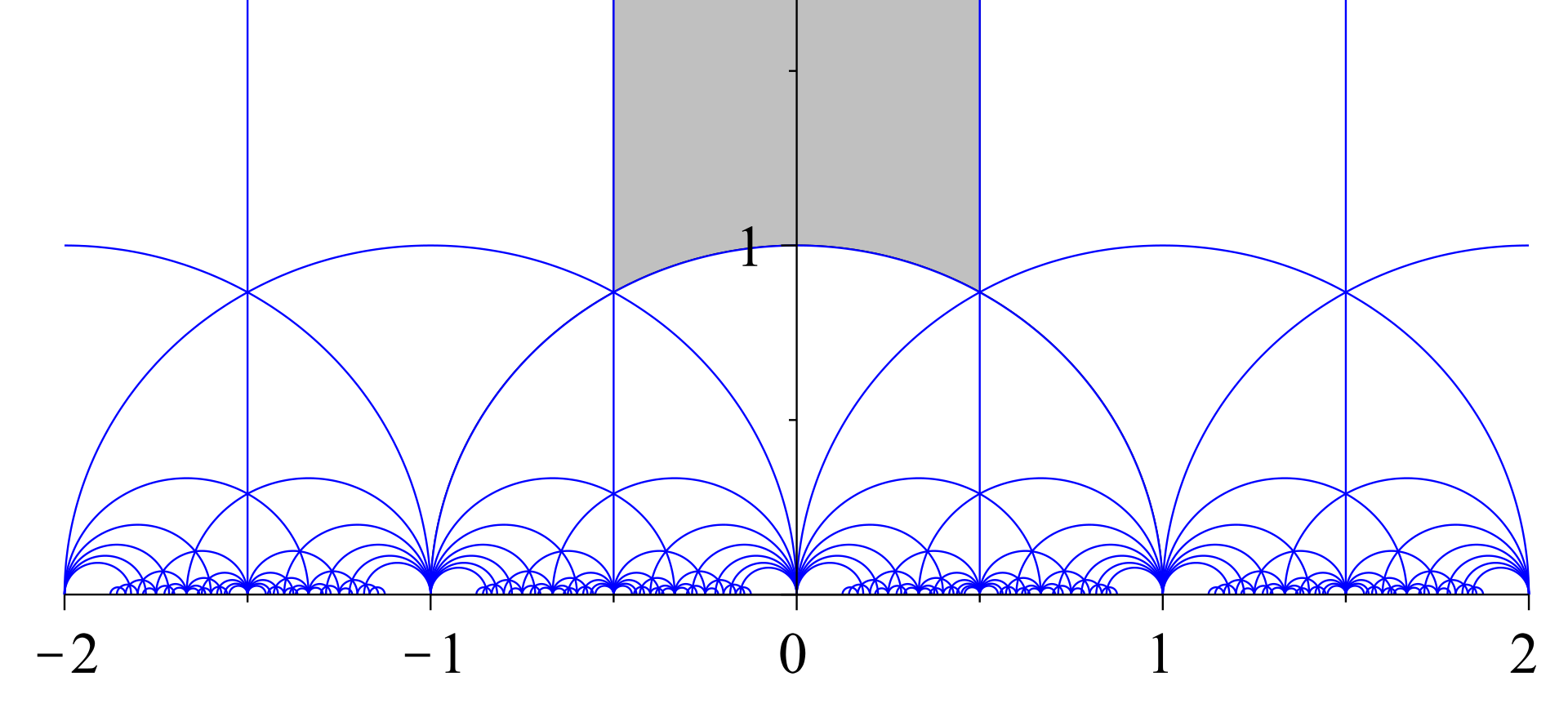
Moreover, fundamental domains for the action of on are represented in Figure 4, which is a famous picture that you can find in so many books of geometry or number theory.
5.2 The curve
So, to parameterise the set of elliptic curves up to isomorphism, we can consider the quotient . It is proved in [Mil17, Prop. 2.21] that this quotient is a complex variety isomorphic to , i.e. to the complex affine line. This is not surprising, Theorem 65 entails that complex elliptic curves up to ismomorphisms are in one-to-one correspondence with via the map , where denotes the –invariant of .
Next, for convenience and in order to apply results on algebraic curves introduced in § 2, it will be useful to have some projective closure of this parameterising curve. In the complex setting, this is nothing but a compactification and the affine line can be compactified with one point. However, for a reason which will appear to be more natural in the sequel, the compactification will be made via a somehow more complicated construction.
The idea is to join to all the elements of which lie on the boundary of together with a point at infinity. Namely, we define
Next let us see how the action of extends to .
Proposition 71.
Consider the following action of on :
This action is transitive, i.e. for any , there exists such that .
Proof.
First, let us prove that the orbit of equals the whole . Note first that
Hence is in the orbit of . Next, consider any other point , i.e. such that . After multiplying the coordinates by a common denominator, one can suppose that and after possibly dividing by their greatest common denominator, one can suppose are prime to each other. By Bézout’s Theorem, there exist such that and then
Therefore, any element of is in the orbit of . Finally, given two elements there exist such that and and . ∎
Therefore, the quotient is nothing but the compactification of by adjoining a single point. This quotient is usually denoted as and is nothing but the Riemann sphere .
In terms of functions on , there exists a holomorphic function which is invariant under the action of and such that the induced map is bijective. This map realises an isomorphism between and . It can be “made explicit” as follows. From construct the lattice . Then using the Weierstrass function, compute an equation of the elliptic curve corresponding to . Then, is nothing but the –invariant of this latter elliptic curve.
5.3 The curve
Once we have a curve parameterising elliptic curves up to isomorphisms, we are still a bit far from our objective since we look for a family of curves whose sequence of genera goes to infinity, while we only got which has genus . To get curves with a higher genus, we need to enhance the structure and the idea is not only to classify elliptic curves up to isomorphism but to classify for a fixed integer , the –isogenies up to isomorphism. In the sequel we are only interested in the case where is prime (but many of the results to follow extend to an arbitrary degree of isogeny).
Remark 72.
Note that, here, by “up to ismomorphism” we mean that two isogenies and will be said to be isomorphic if there exist two isomorphisms and such that the following diagram commutes.
From Theorem 59, an –isogeny corresponds to a pair where is a subgroup of cardinality . Then, in the complex setting, it reduces to classify pairs of lattices such that and . The structure theorem for finitely generated modules over a principal ideal ring asserts that there exists a basis of such that
With the above description, one sees easily that and identifies to an –subspace of dimension of , namely the subspace spanned by the class of . Since we wish to classify elliptic curves with a given –torsion subgroup , we need to classify changes of basis preserving this subgroup. Observe that the action of on bases of induces a natural action of on . The elements of that fix the class of are the upper triangular matrices. This motivates the definition of the congruence subgroup defined as
Namely, this is the group of elements of which induce an automorphism of fixing .
Exercise 73.
Prove that the canonical map
given by the reduction of the coefficients modulo is surjective. To do it:
- (a)
Prove that an element of has a lift with such that are nonzero and prime to each other.
- (b)
Prove that for such a lift, can be replaced by such that and so that
Therefore, the set of –isogenies between elliptic curves up to isomorphism is in one-to-one correspondence with the complex variety
This variety has a compactification
This is a compact Riemann surface and it can be proved that such an object is actually algebraic, i.e. is biholomorphic with a smooth complex projective curve. This structure of algebraic curve is discussed further.
The next statement gives a crucial information, namely the genus of .
Theorem 74.
For a prime number , the genus of equals
We first need two technical lemmas.
Lemma 75.
Let be a prime integer. Let be a lattice and be two distinct lattices both containing and . Suppose that for some . Then and . Equivalently, given an elliptic curve over and two distinct subgroups of cardinality of . If the curves and are isomorphic, then there is an automorphism of sending onto .
Remark 76.
Note that if has such an automorphism, then it should be one of the two curves mentioned in Theorem 69.
Proof of Lemma 75.
Step 1. An adapted basis. We claim that there exists such that
| (21) |
The existence of can be obtained as follows. First, the structure theorem for finitely generated modules over principal ideal rings asserts the existence of a basis such that
Next, we claim that
for some . Indeed, consider , which isomorphic to . In this quotient, and are identified to two –subspaces of dimension in direct sum. The subspace is spanned by the class of and the fact that and are in direct sum in entails that should be spanned by the class of for some . This implies that there exists such that and hence
Then, since , we can deduce that the above inclusion is actually an equality. Finally, define as
Note that the above change of variables is given by a matrix in and provides a basis for which satisfies (21).
Step 2. The modulus of . A classical notion in lattice theory is that of the determinant or volume of the lattice. It can be defined as follows. Consider and regard as a –dimensional –vector space with canonical basis . Since any basis of can be deduced from by applying a matrix in , i.e. a matrix with determinant , the quantity is the same for any basis of . Hence we denote this quantity . From (21), we have
| (22) |
Moreover, the multiplication by map regarded as an –linear endomorphism of has determinant . Indeed, writing , the map is represented in the basis by the matrix
whose determinant is . Next, the assumption together with (22) give
which yields .
Step 3. We aim to prove that . Suppose it does not. Since , and , then . Recall that and is prime. Then, since we assumed that , we get . Similarly, one deduces that . Next, from (21), we see that and hence
By induction,
Therefore, for any , there exists a finite sequence of elements of such that
Then, for any ,
where the ’s are in . When goes to infinity, the right hand side is a convergent series. Thus, so does the left hand side and hence, its general term should go to . From the previous step, we know that and since the ’s are in which is discrete, then for any sufficiently large . Therefore, the sequence of partial sums of the left–hand side is stationary while that of the right–hand side is note. This is a contradiction. Therefore . ∎
Lemma 77.
Let and consider its automorphism group induced by the multiplications by in . Then, any which has a non trivial stabiliser under the action of is in .
Similarly, let , where with its automorphism group induced by the multiplications by , then any with a non trivial stabiliser under the action of is in .
Proof.
In the case , denote by . Since is cyclic of order , its only nontrivial subgroups are and itself. A point stabilised by corresponds to such that . That is to say and hence . Similarly if is stabilised by all it is a fortiori stabilised by and hence should be in .
Consider now the case of . Denote by . Since is cyclic of order , its only possible nontrivial subgroups are , and itself. Let us consider points which are stabilised by one of these groups.
Let stabilised by , then the very same reasoning as for yields .
Let stabilised by . This corresponds to satisfying . Writing for some and using the relation , we get
This entails that
where . By elimination, we deduce that and , that is to say and hence .
Finally, the previous discussion entails that a point stabilised by the whole should be in , and hence is nothing but . ∎
Proof of Theorem 74.
The idea is to consider the projection map , which sends a class of isomorphisms of isogenies onto the isomorphism class of . This map is algebraic (this will appear more naturally in § 5.4). The objective is to apply Riemann Hurwitz formula (Theorem 31) to in order to compute the genus of .
Step 1. The degree of . The degree of is the generic number of pre-images of a point of . Such a point corresponds to a curve up to isomorphism and its pre-image is the set of isomorphism classes of –isogenies or equivalently, the ismomorphism classes of pairs where is a subgroup of cardinality of . From Lemma 75, if has no nontrivial automorphism, then two distinct subgroups provide non isomorphic pairs . Thus, in this situation, the number of pre-images of by corresponds to the number of subgroups of cardinality in . Since is prime, then from Theorem 54, and hence is a vector space of dimension over . Next, a subgroup of cardinality of is nothing but a subspace of dimension and the number of subspaces of dimension (i.e. of lines) of equals . Thus,
Now, the map is ramified at the points corresponding to curves with nontrivial automorphisms and possibly the point at inifinity. From Theorem 69, the curves with nontrivial automorphisms correspond to the tori and , where . For these tori, we need to understand the action of the automorphisms on the –torsion.
Step 2. Ramification at . The curve is equipped with a nontrivial automorphism of order , which corresponds to the multiplication by in . This automorphism acts on the –torsion and, from [Sil09, Thm. III.4.8], such an automorphism is a group automorphism and hence its action on regarded as an –vector space is –linear. We denote by , the automorphism restricted to . From Lemma 77, since any point in has has an orbit of cardinality under . Therefore, has order and two situations may occur. Either , then contains fourth roots of and regarded as an –automorphism of is diagonalisable as
where denotes a primitive fourth root of . In this situation, acts on the lines of by fixing the two lines corresponding to the eigenspaces of and any other line has an orbit of cardinality , indeed , which leaves any line invariant. Two lines of in a same orbit under correspond to a same point in . This point is a ramification point with ramification index . Therefore, if , then there are unramified points in the pre-image of the isomorphism class of by and ramified points with ramification index .
Otherwise . In this situation has no eigenspace in and the orbit of any line has cardinality . Thus, there are points above which are all ramified with ramification index .
Step 3. Ramification at . Here we have an automorphism of order and denote again by its restriction to . Here again, from Lemma 77, we know that has also order . In this situation, if , then contains sixth roots of unity and is diagonalisable. Therefore, the two eigenspaces of are left invariant and any other –line of has an orbit of cardinality . Indeed, here again and hence leaves any line globally invariant. In such a situation, the pre-image of consists in unramified points corresponding to the two eigenspaces of in and points with ramification index .
If , then any line of has an orbit of cardinality under the action of and hence the pre-image of by consists in points, all with ramification index .
Step 4. Ramification at infinity. The point at infinity of is the quotient of under the action of , which, from Proposition 71, consists in a single orbit. We wish to estimate the number of orbits in under the action of . We claim that their number is , namely, the orbit of and that of . Indeed,
and
One easily sees that the two orbits form a partition of . This entails that the pre-image of the point at infinity of consists in two points whose ramification indexes satisfy .
Final step. Computation of the genus. Denote by the genus of and by that of Riemann–Hurwitz formula asserts that
where and are the respective contributions of the ramifications above , and the point at infinity. We get
An easy but cumbersome calculation treating separately the four cases yields the expected result. ∎
5.4 The modular equation
To conclude this section, we give a statement whose proof is omitted but which may help the reader to be convinced that has a structure of algebraic curve. We refer the reader to [Mil17, Thm. 6.1] for a proof.
Theorem 78.
There exists an irreducible polynomial such that for any pair of elliptic curves related with a degree isogeny , then .
Remark 79.
A database of the polynomials for small values of is available on Andrew Sutherland’s webpage: https://math.mit.edu/drew/ClassicalModPolys.html
Let us give some comments about this statement. First, note that the projective closure of the complex curve of equation is a “singular model” for . Indeed, any point of corresponds to an isomorphism class of –isogeny . This yields a rational map
The image of this map is contained into the curve with equation . However, this latter curve is full of singularities and hence is not isomorphic to . Nevertheless, (and this is far from being obvious) this permits to deduce that is itself defined over and hence, its reduction modulo makes sense.
An interesting fact is that, since , for any pair of –isogenous curves over we have . Moreover, if and are prime to each other, it is known that the polynomial is irreducible modulo (see for instance [Mor90, Thm. 5.9]). Thus, the curve over of equation turns out to be a singular model of a smooth curve over , that we will also denote by such that parameterises –isogenies over up to isomorphism. These curves over will be the objects of interest in order to prove the main theorem of this course, namely Theorem 41.
6 Proof of the main Theorem
Now, we almost have the material to prove Theorem 41. We have our family of curves for a prime integer distinct from the characteristic .
6.1 Genus of modular curves over finite fields
Let us briefly discuss the genus of the curve. The discussion to follow is far from being trivial. Thus, the reader is encouraged first to directly admit the conclusion. Namely that the genus of a modular curve over a finite field is that of its complex counterpart. Let us briefly sketch the reasons why this holds.
It is known (see for instance in [Mor90, Thm. 5.9]) that, the curve has a smooth projective model described by equation with coefficients in and whose reduction modulo is smooth too.
Next, as already mentioned in Remark 29, two different notions of genus are associated to a curve, the arithmetic genus and the geometric one . The genus introduced by Definition 25 in § 2.7 is the geometric one. The arithmetic genus, which can be defined for instance from the Hilbert function of the variety [Har77, Ch. IV], is always larger than or equal to the geometric one and they coincide if and only if the curve is smooth.
Next, Grauert Theorem [Har77, Cor. III.12.9] permits to assert that the reduction modulo of the aforementioned model has the same arithmetic genus as the complex curve itself. Moreover, since this model and its reduction are smooth, they also have the same geometric genus. Therefore, the genus of the curve over is the same as that of its complex counterpart and hence is given by Theorem 74.
6.2 The locus of supersingular curves
There remains to get an estimate of the number of rational points of such curves. For this we will focus on –points since their number can be bounded from below using the two following statements.
Proposition 80.
Let be a supersingular elliptic curve over , then is defined over .
Proof.
By definition, a supersingular curve satisfies . Therefore, the multiplication by map is totally inseparable.
Consider now the Frobenius map
It is a degree isogeny, hence it has a dual isogeny such that . Since is totally inseparable, should be inseparable either and hence, so should be the Frobenius map
Thus, and hence is defined over . ∎
Theorem 81.
The number of –isomorphism classes of supersingular elliptic curves over equals
Proof.
See [Sil09, Thm. V.4.1]. ∎
6.3 Proof of the main theorem
With these two last statements at hand we can finally provide the proof of Theorem 41. We restrict the proof to the case . Note that Tsfasman–Vlăduţ–Zink theorem remains true when but the coding theoretic interest is rather limited.
Proof of Theorem 41.
Consider the sequence of curves for . From Theorem 74 it has genus . From Theorem 81, the curve has at least –rational points corresponding to isomorphism classes of supersingular elliptic curves. Such an elliptic curve with no nontrivial automorphism has pre-images in which also correspond to supersingular elliptic curves and hence are –rational points. Depending on the class of modulo the curves with –invariant and may be supersingular. More precisely, from [Sil09, Ex. V.4.4 & V.4.5],
- •
for , both curves are ordinary (i.e. non supersingular) and then any supersingular curve has no nontrivial automorphism and hence has pre-images in . Therefore, from Theorem 81,
- •
for , the curve with is supersingular and the one with is ordinary. Therefore, there are supersingular curves and all of them but one have distinct pre-images. The remaining curve is the one with and an automorphism group of order . Its treatment is very similar to the proof of Theorem 74. Consider the action of the automorphism of order on the –torsion. From Lemma 77, this induces an automorphism or order of . Since , then and hence does not contains the sixth roots of unity. Thus, is not diagonalisable and hence cannot fix a line. Consequently, one proves that the orbit of any line is the union of distinct lines (, which fixes the lines). Therefore, the curve with –invariant has pre-images and Consequently, using Theorem 81:
- •
for , the curve with is ordinary and the one with is supersingular. A similar reasoning yields
- •
for , both curves are supersingular and we get:
In summary, we always have a lower bound on the number of rational points. Then
Thus, over for , we identified a family of curves whose number of –rational points goes to infinity and whose ratio, number of –points divided by the genus goes to . Which turns out to be optimal. ∎
References
- [BH08] Peter Beelen and Tom Høholdt. The decoding of algebraic geometry codes. In Advances in algebraic geometry codes, volume 5 of Ser. Coding Theory Cryptol., pages 49–98. World Sci. Publ., Hackensack, NJ, 2008.
- [Cou16] Alain Couvreur. Introduction to coding theory, 2016. Personal lecture notes.
- [CR21] Alain Couvreur and Hugues Randriambololona. Algebraic geometry codes and some applications. In W. Cary Huffman, Jon-Lark Kim, and Patrick Solé, editors, Concise Encyclopedia of Coding Theory. Chapman and Hall/CRC, 2021.
- [DR73] P. Deligne and M. Rapoport. Les schémas de modules de courbes elliptiques. In Modular functions of one variable, II (Proc. Internat. Summer School, Univ. Antwerp, Antwerp, 1972), Lecture Notes in Math., Vol. 349, pages 143–316. Springer, Berlin, 1973.
- [Duu08] Iwan M. Duursma. Algebraic geometry codes: general theory. In Advances in algebraic geometry codes, volume 5 of Ser. Coding Theory Cryptol., pages 1–48. World Sci. Publ., Hackensack, NJ, 2008.
- [Ful89] William Fulton. Algebraic curves. Advanced Book Classics. Addison-Wesley Publishing Company Advanced Book Program, Redwood City, CA, 1989. An introduction to algebraic geometry, Notes written with the collaboration of Richard Weiss, Reprint of 1969 original.
- [Gop81] Valerii D. Goppa. Codes on algebraic curves. Dokl. Akad. Nauk SSSR, 259(6):1289–1290, 1981. In Russian.
- [GS95] Arnaldo Garcia and Henning Stichtenoth. A tower of Artin-Schreier extensions of function fields attaining the Drinfeld-Vladut bound. Inventiones Mathematicae, 121:211–222, 1995.
- [Har77] Robin Hartshorne. Algebraic geometry, volume 52 of Graduate Texts in Mathematics. Springer-Verlag, New York, 1977.
- [HP95] Tom Høholdt and Ruud Pellikaan. On the decoding of algebraic–geometric codes. IEEE Trans. Inform. Theory, 41(6):1589–1614, Nov 1995.
- [HvLP98] Tom Høholdt, Jacobus Hendricus van Lint, and Ruud Pellikaan. Algebraic geometry of codes. In Handbook of coding theory, Vol. I, II, pages 871–961. North-Holland, Amsterdam, 1998.
- [Iha81] Y. Ihara. Some remarks on the number of rational points of algebraic curves over finite fields. J. Fac. Sci. Univ. Tokyo Sect. IA Math., 28:721–724, 1981.
- [KM85] Nicholas M. Katz and Barry Mazur. Arithmetic moduli of elliptic curves, volume 108 of Annals of Mathematics Studies. Princeton University Press, Princeton, NJ, 1985.
- [Lor96] Dino Lorenzini. An invitation to arithmetic geometry, volume 9 of Graduate Studies in Mathematics. American Mathematical Society, Providence, RI, 1996.
- [LPS88] A. Lubotzky, R. Phillips, and P. Sarnak. Ramanujan graphs. Combinatorica, 8(3):261–277, 1988.
- [Mar88] G. A. Margulis. Explicit group-theoretic constructions of combinatorial schemes and their applications in the construction of expanders and concentrators. Problemy Peredachi Informatsii, 24(1):51–60, 1988.
- [Mil17] James S. Milne. Modular functions and modular forms (v1.31), 2017. Available at www.jmilne.org/math/.
- [Mor90] Carlos J. Moreno. Algebraic curves over finite fields. Cambridge tracts in mathematics. Cambridge University Press, Cambridge, 1990.
- [Sha94] Igor R. Shafarevich. Basic algebraic geometry. 1. Springer-Verlag, Berlin, second edition, 1994.
- [Sil09] Joseph Silverman. The arithmetic of elliptic curves, volume 106. Springer-Verlag New York, second edition, 2009.
- [Ste99] Serguei A. Stepanov. Codes on algebraic curves. Kluwer Academic/Plenum Publishers, New York, 1999.
- [Sti09] Henning Stichtenoth. Algebraic function fields and codes, volume 254 of Graduate Texts in Mathematics. Springer-Verlag, Berlin, second edition, 2009.
- [TVN07] Michael A. Tsfasman, Serge Vlăduţ, and Dmitry Nogin. Algebraic geometric codes: basic notions, volume 139 of Mathematical Surveys and Monographs. American Mathematical Society, Providence, RI, 2007.
- [TVZ82] Michael A. Tsfasman, Serge G. Vlăduţ, and Th. Zink. Modular curves, Shimura curves, and Goppa codes, better than Varshamov-Gilbert bound. Math. Nachr., 109:21–28, 1982.
- [VD83] Sergei G. Vlăduţ and Vladimir G. Drinfeld. Number of points of an algebraic curve. Funct. Anal. Appl., 17:53–54, 1983.
- [VM84] S. G. Vlăduţ and Yu. I. Manin. Linear codes and modular curves. In Current problems in mathematics, Vol. 25, Itogi Nauki i Tekhniki, pages 209–257. Akad. Nauk SSSR Vsesoyuz. Inst. Nauchn. i Tekhn. Inform., Moscow, 1984.
- [Wal00] Judy L. Walker. Codes and curves, volume 7 of Student Mathematical Library. American Mathematical Society, Providence, RI; Institute for Advanced Study (IAS), Princeton, NJ, 2000. IAS/Park City Mathematical Subseries.