Simplifying Open-Set Video Domain Adaptation with Contrastive LearningJournal: Computer Vision and Image Understanding
Abstract
In an effort to reduce annotation costs in action recognition, unsupervised video domain adaptation methods have been proposed that aim to adapt a predictive model from a labelled dataset (i.e., source domain) to an unlabelled dataset (i.e., target domain). In this work we address a more realistic scenario, called open-set video domain adaptation (OUVDA), where the target dataset contains “unknown” semantic categories that are not shared with the source. The challenge lies in aligning the shared classes of the two domains while separating the shared classes from the unknown ones. In this work we propose to address OUVDA with an unified contrastive learning framework that learns discriminative and well-clustered features. We also propose a video-oriented temporal contrastive loss that enables our method to better cluster the feature space by exploiting the freely available temporal information in video data. We show that discriminative feature space facilitates better separation of the unknown classes, and thereby allows us to use a simple similarity based score to identify them. We conduct thorough experimental evaluation on multiple OUVDA benchmarks and show the effectiveness of our proposed method against the prior art.
MSC
41A05, 41A10, 65D05, 65D17 \KWDKeyword1, Keyword2, Keyword31 Introduction
Action recognition is an important problem in the field of computer vision where the task consists in recognizing the action being performed in a video sequence. Supervised action recognition (Tran et al. 2015; Feichtenhofer et al. 2016; Carreira and Zisserman 2017; Zhou et al. 2018) is widely studied because of the growing need for automatically categorizing video content that are being generated everyday. However, it is nearly impossible for human annotators to keep pace with the enormous volumes of online videos, and thus supervised training becomes infeasible. A cheaper way of leveraging the massive pool of unlabelled data is by exploiting an already trained model to infer the labels on such data and then re-using them to build an improved model. Such an approach is also prone to failure because the unlabelled data may belong to a data distribution that is different from the annotated one, which is often referred to as the domain-shift problem (Torralba and Efros 2011).
To address the domain-shift problem, Unsupervised Video Domain Adaptation (UVDA) methods (Chen et al. 2019; Choi et al. 2020; Pan et al. 2020) have been proposed that aim to learn a model for the domain of interest by jointly leveraging the annotated source data and the unannotated target data. However, these methods make a strong and unrealistic assumption that the source and target domains share the same label space, which is also known as the closed-set scenario. The closed-set assumption is rarely the case in the real world as the target domain can contain video sequences from action categories that are not present in the source dataset. Such non-overlapping categories are known as the out-of-distribution (OOD) classes (Vaze et al. 2022). A naive application of the existing UVDA techniques will cause the model to incorrectly classify the OOD classes as one of the shared ones, which is undesirable.
Due to the limited applicability of the closed-set UVDA setting, the focus has been shifting towards the more challenging open-set scenario where the target dataset contains samples associated with categories that are not present in the source domain. In the context of action recognition, this task is referred to as the Open-Set Unsupervised Video Domain Adaptation (OUVDA) (Chen et al. 2021). The main goal in OUVDA consists in adapting a model to the target domain that can align the classes that are shared between the two domains while excluding the OOD (also known as target-private or unknown) classes from the alignment process. Although open-set unsupervised domain adaptation has received significant attention for the image classification task (Saito et al. 2018b; Saito et al. 2020; Bucci et al. 2020; Saito and Saenko 2021; Bucci et al. 2021), it is rather understudied in the field of action recognition (Chen et al. 2021).
The recently proposed OUVDA method, CEVT (Chen et al. 2021), uses a weighted adversarial learning strategy, with the weights derived from class-conditional extreme value theory, in order to recognize the target-private classes. However, adversarial learning-based alignment can be unstable in practice, especially in the open-set scenarios. In this work, we argue that OUVDA can be greatly simplified if we can learn discriminative features on both the source and target data for the following two reasons: (i) it can implicitly align the shared classes between the source and target domains by learning semantically distinct clusters (Wang and Isola 2020); and (ii) it results in the target-private classes being well separated from the shared ones (see Fig. 1). Based on this intuition, we propose to leverage contrastive learning (Gutmann and Hyvärinen 2010; Chen et al. 2020; He et al. 2020) to obtain discriminative representations to tackle OUVDA.
In details, we realize the above goals by proposing to use different instantiations of the contrastive loss that mainly differ in how the positives and negatives are mined. To recap, the contrastive loss (Chen et al. 2020) relies on positives and negatives which are then contrasted to learn feature representation. In our proposed method we use four such instantiations of contrastive loss: (i) a label-based supervised contrastive loss for the source; (ii) an augmentation-based contrastive loss for the target; (iii) a cross-domain contrastive loss between the source and the pseudo-labelled target; and (iv) a temporal contrastive loss to learn the temporal dynamics present in video data. One important advantage with such a proposal is that we can leverage an unique contrastive formulation to unify several losses, which cater to different learning aspects of the task at hand. It also ensures compatible gradients and dispose of the need of tuning several hyperparameters. To this end, we call our proposed method COLOSEO (COntrastive Learning for Open-SEt VideO Domain Adaptation).

Owing to the well-clustered feature space we observe that it becomes fairly straightforward to separate the target-private instances from the shared ones. In this work we use the nearest class prototypes (Mensink et al. 2013) with a simple cosine-similarity metric to exclude the target-private instances from the alignment process that lie far from all the source classes prototypes. We extensively validate our proposed method on multiple benchmarks: (i) HMDBUCF and UCFOlympic that contains actions from third-person view; and (ii) the challenging first-person (egocentric) Epic-Kitchens.
Contributions
To summarize, our main contributions are: (i) the COLOSEO framework, which uses an unified contrastive learning formulation to address the task of OUVDA. We demonstrate that learning compact and discriminative feature representations can greatly simplify the OUVDA task; (ii) a novel video-oriented temporal contrastive loss that improves the OOD robustness, thereby facilitating the task at hand; (iii) we advance the state-of-the-art on three standard OUVDA benchmarks by non-trivial margins.
2 Related Works
Open-set Unsupervised Domain Adaptation
There exists a large body of the open-set unsupervised domain adaptation (OUDA) literature but applied specifically to the image classification task. OUDA was first introduced by Panareda Busto and Gall 2017 and later then addressed in several subsequent works, which mostly rely either on adversarial learning or clustering approaches.
Most of the initial works (Saito et al. 2018b; Shermin et al. 2021) exploited adversarial learning to detect target-private samples while aligning features of different domains for the known categories. Fu et al. 2019 improved the adversarial objective of Saito et al. 2018b by replacing the binary cross entropy loss with a symmetrical Kullback-Leibler distance-based loss. Liu et al. 2019 addressed OUDA by training a multi-binary classifier with source data, alongside domain discriminator, to progressively separate the samples of unknown and known classes. A graph neural network based approach was proposed by Luo et al. 2020 that integrates episodic pseudo-labelling with adversarial learning to tackle the OUDA task.
Recently, the adversarial approaches have been replaced by clustering-based methods (Wang 2021) that ensure well clustered target space. For instance, Bucci et al. 2021 proposed HyMOS that uses contrastive learning to enforce invariance to the augmentations obtained via style transfer. However, HyMOS is tailored for the multi-source OUDA setting. Ma et al. 2021 introduced a method for active OUDA that combines adversarial learning with the clustering non-transferable gradient embedding approach. Recently, Saito et al. 2020 proposed DANCE that uses self-supervision to cluster the target data, followed by detecting the target-private instances based on the entropy computed by the classifier. Different to all other approaches, OVANet (Saito and Saenko 2021) trains one-vs-all binary open set classifiers on the source data to detect and reject the unknown samples. A common theme in all these above methods is that they are have been proposed for images and do not exploit the temporal information which video data has to offer.
Open-set Unsupervised Video Domain Adaptation
In the realm of action recognition the open-set video domain adaptation (OUVDA) the literature is relatively under explored. Busto et al. 2019 proposed a generic approach based on learning a mapping from the source to the target domain and learning an open-set classifier on the mapped samples. CEVT was introduced by Chen et al. 2021 that models the entropy of the target samples as generalised extreme value distribution in order to perform open-set separation. Differently from the prior art CEVT, our proposed approach additionally exploits the temporal dynamics in the video sequences. We observe that modelling the temporal dynamics can lead to better representations, which leads to even compact action clusters. Moreover, the adopted contrastive learning objective allows us to align the two domains without the need of any adversarial feature alignment.
Contrastive Representation Learning
As collecting annotated data is costly, the research community has focused on self-supervised representation learning (SSL) that learns discriminative features unsupervisedly with the help of a pretext task. Contrastive learning (Gutmann and Hyvärinen 2010; Chen et al. 2020; He et al. 2020) is one such family of SSL methods that casts the learning as an instance discrimination task where the similarity between two correlated views are maximized. So far in the literature, contrastive learning has recently been exploited in an attempt to learn discriminative features, but only in the context of closed-set UVDA (Munro and Damen 2020; Kim et al. 2021; Sahoo et al. 2021; Turrisi da Costa et al. 2022a; Turrisi da Costa et al. 2022b). Moreover, contrastive learning has found to be effective for detecting OOD images samples (Winkens et al. 2020). Different from these works, our proposed formulation of different contrastive losses takes into account the temporal dimension in video. In our experiments we show that the proposed temporal contrastive loss is influential in improving over the image-based counterparts.
3 Methods
In this work, we propose COLOSEO for addressing the Open-set Unsupervised Video Domain Adaptation (OUVDA) task. We first formally define OUVDA and then we introduce our proposed method.
Problem Definition and Notations
Let us assume that there is a labelled source dataset containing instances, where represents an input and the corresponding semantic categories. We also assume that there is an unlabelled target dataset of instances, containing the shared semantic categories of the source dataset and some additional categories, denoted as target-private or unknown classes11 1 In this work target-private and unknown classes are used interchangeably, which are absent in the . These unknown classes are designated as the th class. As per standard unsupervised domain adaptation assumption, the underlying marginal probability distributions between the source and the target domains differ from each other, i.e., . Under such conditions, the goal in the OUVDA is to learn a mapping , modelled by a neural network with parameters , that can correctly classify the shared instances of the into the first classes and all the target-private instances into the th class.
Since we are working with arbitrary-length video sequences, during training, we sub-sample frames from each video sequence to form constant-length clips. More formally, each input sample is given as , where denotes the number of frames used in constructing the clip. As it is done typically in the action recognition pipelines, clips from a video sequence are presented as input to and then later summarized (or aggregated) to provide the final class prediction.
Overview
In this work we propose to simplify the OUVDA task by resorting to contrastive learning (Chen et al. 2020; He et al. 2020). We choose contrastive learning because it learns very discriminative representations that are often useful for several downstream tasks (Ericsson et al. 2021). Moreover, it has also been shown in the work by Saito et al. 2020 that learning discriminative representations greatly alleviates the misalignment problem between the shared and unknown classes owing to the well-structured feature space. Furthermore, self-supervised representation learning has been found useful for detecting OOD samples (Hendrycks et al. 2019), which is also a key constituent challenge in the OUVDA.
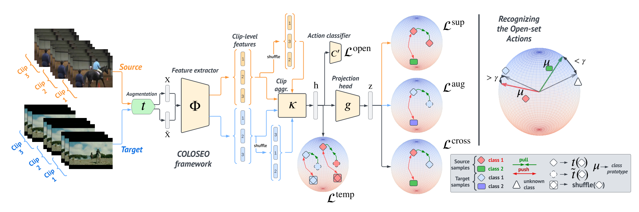
Our proposed COLOSEO is divided into two stages. In the first stage, we aim at learning useful video-level feature representations on both the source and the target data such that instances with the same underlying action are clustered together, facilitating the adaptation phase. Since the source data is labelled we use both the standard cross-entropy classification loss and the supervised contrastive loss (Sup-Con) (Khosla et al. 2020), such that instances from the same class are pulled closer to each other, while instances from different class are pushed apart. As the target data lack labels, we adopt the augmentation-based SimCLR (Chen et al. 2020) loss to cluster the instances in the target domain. Lastly, as temporal dynamics are crucial for distinguishing between different actions, we propose a temporal contrastive loss that contrasts between non-shuffled and shuffled clips in a given video sequence. The temporal contrastive loss allows the network to learn the salient temporal dynamics in an action, which is important for the recognition of the action (see Fig. 2 left).
The second stage deals with further aligning the feature representations of the source and target domains, while ensuring that the target-private instances are not aligned with the shared classes. To this end, we introduce a simple score-based nearest prototype classifier which determines if a target sample belongs to the shared classes or not. This score is measured with respect to the source prototypes (or class centroids) in order to be less prone to noisy outliers (see Fig. 2 right). If a target sample is deemed to belong to one of the shared classes, we find its pseudo-label with the help of the closed-set source classifier and employ the Sup-Con loss to align the source and the target representations. On the other hand, if the target sample is detected to be far from all the source prototypes, it is then excluded from the cross-domain feature alignment. A -way classifier is learned in the second stage that additionally classifies the detected target-private instances into the th class. An overview of our method is provided in the Fig. 2, and we describe it in detail below.
3.1 COLOSEO: Contrastive Learning for OUVDA
To address the OUVDA, we employ contrastive learning (Chen et al. 2020; He et al. 2020) in both the stages to (i) produce discriminative feature representations for both the source and target data; and (ii) align the source and target domains over the shared classes. We realize the above goals by using four different versions of the contrastive losses that differ in a way the positives and negatives are created, which are: (i) the label-based Sup-Con (Khosla et al. 2020) , where positives consist of samples with the same class label and negatives are the samples with a different class label; (ii) the augmentation-based contrastive loss where the positives are the augmented views of a given sample, and negatives consist of all other samples in the mini-batch; (iii) the temporal contrastive loss where the positives are the same as in the augmentation-based loss, but the negatives are created by shuffling the order of the clips of the same video; and (iv) the cross-domain contrastive loss which is similar to the , except that the pseudo-labels are utilized for the unlabelled target samples.
Given a mini-batch of source domain video sequences and target domain video sequences of size , we apply two stochastic data augmentation transformations and on each sample to create the positive pairs (or views) as , and , . As each video sequence consists of clips, we first forward the clips through the feature extractor to obtain clip-level features, which are then fused using the clip aggregator network . In detail, for every input video sequence the aggregator network yields a video-level feature . Thus, corresponding to the positive pairs , and , in the input space we have and in the video-level feature space . Following, the previous works on self-supervised learning (Chen et al. 2020; Khosla et al. 2020), we also use a non-linear projection head that operates on the video-level features producing .
Label-based Contrastive Loss
Since the source data is annotated, we exploit the class label information to create more informative positives and negatives. In detail, given an instance belonging to the class , another instance is a positive in the mini-batch if it shares the same class label, i.e., . Similarly, all other instances in the mini-batch which do not share the same class label with are considered negatives. The label-based contrastive loss is then defined, for the th source sample, as:
where , is the dot product between the L2 normalized and and is a temperature parameter. The operator evaluates to 1 with or 0 otherwise. Similarly, the operator yields 1 if the class labels are different, or 0 otherwise.
Augmentation-based Contrastive Loss
For the unlabelled target data, we use the augmentation-based contrastive loss. Given an instance , its positive is defined as the augmented view of itself and its negatives are all the other instances in the mini-batch. We can define the augmentation-based contrastive loss on the th target sample as:
| (4) |
We make the loss symmetric by swapping and and averaging the losses.
Temporal Contrastive Loss
While the self-supervised contrastive loss is very much potent at modelling the shapes of objects in the clips while ignoring the low-level appearance information, it still might not be sufficient in the case of action recognition due to the temporal dynamics associated with an action. Consider an example, where the network must discriminate between the actions “push-up” and “pull-up”. Since both these classes depict humans performing work-out routines, the invariances induced by the strong augmentations in the contrastive loss would favour discovering the human shape, which is confounding for the two action classes. However, the classes “push-up” and “pull-up” inherently exhibit different temporal dynamics, which are unique of their own. We conjecture that, asides from modelling the shape with the contrastive loss, capturing the temporal dynamics can lead to even more discriminative features. Thus, in order to benefit from the temporal information inherently conveyed in video data, we design a video-oriented temporal contrastive loss that contrasts between video sequences with shuffled and non-shuffled clips.

As before, given a sample , we create its positive view with the help of a strong augmentation. Whereas, for contrasting with a regular video sequence, we artificially generate negatives by randomly permuting the order of clips in , producing . However, as the contrastive loss requires a significant amount of negatives in a mini-batch to work (Chen et al. 2020; He et al. 2020), one would need perform repeated forward passes through the clip aggregator network for every permutation. To circumvent this, we simplified the contrastive formulation to a triplet loss (Chechik et al. 2010), which achieves a similar effect. Then, the goal is to push the anchor close to the augmented sequence , while pushing away from the shuffled (see Fig. 3) in the feature space. The temporal contrastive loss for the th sample is given as:
| (5) |
where is a distance function defined as , where indicates the margin of the triplet loss.
Cross-domain Contrastive Loss
While the aforementioned contrastive losses can lead to a well-clustered feature space, they do not guarantee that the source and target class clusters are perfectly aligned. This is primarily caused by domain shift. To further align the two domains, we propose to use a cross-domain contrastive loss that is similar to the label-based contrastive loss , except that pseudo-labels are used for the unlabelled target samples. In particular, to align a target sample with the source samples, we first infer the pseudo-label of the th target sample using the source classifier . Then we proceed as in Eq. (3.1) to define the cross-domain contrastive loss as:
While inferring the pseudo-label of a target sample with the -way source classifier may work seamlessly in the closed-set UVDA, it is problematic in the OUVDA case because of the presence of the target-private classes. To prevent the target-private classes from being assigned to one of the shared categories, we present an unknown class detection protocol that eliminates the target samples that are unlikely to belong to one of the shared classes. Next we elaborate the unknown class detection protocol.
3.2 Recognizing the Open-set Actions
Before the pseudo-labels are inferred for the target samples, we need a mechanism that can automatically detect the target-private classes. For this purpose, we design a metric which assigns a score to each target sample. A low score means that the target sample’s representation is far from the training data, and is likely to be a target-private instance. For this purpose, we use cosine similarity as the metric between the target feature and the nearest source class prototype. The class prototype for a source class is obtained by averaging the features of all the training samples of class , which is defined as:
| (9) |
where is the number of source samples from the class . If the target feature is farther than its nearest source class prototype by a threshold , i.e., it has cosine similarity lower than the , we consider this sample as target-private. Thus, we have an indicator variable which is 1 if a target sample is target-private and 0 otherwise. We can define it formally as:
| (10) |
where all the target samples with are not included in the cross-domain contrastive loss .
Since the final goal in the OUVDA is not only to classify the shared target instances into one of the classes but also to classify all the target-private instances into the th class, we initialize a -way classifier in the second stage of training. All the target samples where using Eq. (10) are assigned an “unknown” label . We then use a standard cross-entropy loss to assign a high likelihood to the target private instances to be belonging to the th class. Whereas, for the source samples we keep the standard classification loss. The cross-entropy loss is for a source and target-private instance is defined as:
| (11) |
where is the softmax function for normalizing the network logits into a probability distribution. Note that in Eq. (11), for a target-private instance , we backpropagate only for the th class.
Overall objective
We train our model with a mini-batch using the following final objective:
| (12) |
where is a weight for the temporal contrastive loss.
Inference. During inference the classifier is used for classifying the target samples into one of the known or the unknown th category.
4 Experiments
4.1 Experimental Set-up
Benchmarks
We evaluate our proposed framework under the OUVDA task on four benchmarks that are derived from UCF101 (Soomro et al. 2012), HMDB (Kuehne et al. 2011), Olympic Sports (Niebles et al. 2010) and Epic Kitchens (Damen et al. 2018) action recognition datasets. The four benchmarks are described below.
| Method | Backbone | HMDBUCF | UCFHMDB | ||||||
|---|---|---|---|---|---|---|---|---|---|
| ALL | UNK | HOS | ALL | UNK | HOS | ||||
| DANN (Ganin et al. 2015) + OSVM (Jain et al. 2014) | ResNet101 | 64.6 | 62.9 | 74.7 | 68.3 | 66.1 | 48.3 | 83.9 | 61.3 |
| JAN (Long et al. 2016) + OSVM (Jain et al. 2014) | 61.5 | 62.9 | 73.8 | 67.9 | 61.1 | 47.8 | 74.4 | 58.2 | |
| AdaBN (Li et al. 2018) + OSVM (Jain et al. 2014) | 62.9 | 58.8 | 73.3 | 65.3 | 62.9 | 58.8 | 73.3 | 65.3 | |
| MCD (Saito et al. 2018a) + OSVM (Jain et al. 2014) | 66.7 | 63.5 | 73.8 | 68.3 | 66.7 | 57.8 | 75.6 | 65.5 | |
| TA2N (Chen et al. 2019) + OSVM (Jain et al. 2014) | 63.4 | 61.3 | 79.0 | 69.1 | 65.3 | 56.1 | 74.4 | 64.0 | |
| TA3N (Chen et al. 2019) + OSVM (Jain et al. 2014) | 60.6 | 58.4 | 82.5 | 68.4 | 62.2 | 53.3 | 71.7 | 61.2 | |
| OSBP (Saito et al. 2018b) + AvgPool | 64.8 | 55.3 | 85.7 | 67.2 | 67.2 | 50.8 | 84.5 | 63.5 | |
| CEVT (Chen et al. 2021) | 70.6 | 66.8 | 84.3 | 74.5 | 75.3 | 56.1 | 94.5 | 70.4 | |
| OVANet (Saito and Saenko 2021) | I3D | 80.8 | 90.4 | 76.0 | 82.6 | 70.6 | 67.0 | 71.4 | 69.6 |
| CEVT (Chen et al. 2021) | 67.6 | 59.7 | 93.0 | 72.7 | 80.1 | 60.3 | 96.1 | 74.1 | |
| COLOSEO- (ours) | 79.3 | 87.5 | 80.8 | 84.0 | 82.2 | 80.6 | 84.4 | 82.5 | |
| COLOSEO (ours) | 78.3 | 81.1 | 88.7 | 84.7 | 89.1 | 76.7 | 98.9 | 86.4 | |
| Method | Backbone | UCFOlympic | OlympicUCF | ||||||
|---|---|---|---|---|---|---|---|---|---|
| ALL | UNK | HOS | ALL | UNK | HOS | ||||
| DANN (Ganin et al. 2015) + OSVM (Jain et al. 2014) | ResNet101 | 94.4 | 96.7 | 91.3 | 93.9 | 83.3 | 86.4 | 80.6 | 83.4 |
| JAN (Long et al. 2016) + OSVM (Jain et al. 2014) | 94.4 | 100.0 | 87.0 | 93.0 | 88.7 | 80.5 | 95.5 | 87.3 | |
| AdaBN (Li et al. 2018) + OSVM (Jain et al. 2014) | 87.0 | 78.5 | 100.0 | 87.9 | 84.1 | 76.9 | 89.5 | 82.8 | |
| MCD (Saito et al. 2018a) + OSVM (Jain et al. 2014) | 87.0 | 86.7 | 87.0 | 86.8 | 83.7 | 85.5 | 82.1 | 83.8 | |
| TA2N (Chen et al. 2019) + OSVM (Jain et al. 2014) | 96.3 | 100.0 | 91.3 | 95.4 | 87.9 | 78.5 | 95.5 | 86.2 | |
| TA3N (Chen et al. 2019) + OSVM (Jain et al. 2014) | 88.9 | 87.9 | 91.0 | 89.6 | 85.8 | 85.6 | 85.8 | 85.7 | |
| OSBP (Saito et al. 2018b) + AvgPool | 96.9 | 94.4 | 100.0 | 97.1 | 89.0 | 84.3 | 92.0 | 88.0 | |
| CEVT (Chen et al. 2021) | 98.1 | 97.0 | 100.0 | 98.5 | 89.2 | 86.4 | 91.0 | 88.7 | |
| OVANet (Saito and Saenko 2021) | I3D | 80.8 | 90.4 | 76.0 | 82.6 | 70.6 | 67.0 | 71.4 | 69.6 |
| CEVT (Chen et al. 2021) | 81.4 | 67.2 | 100.0 | 80.4 | 90.8 | 84.3 | 96.2 | 89.9 | |
| COLOSEO- (ours) | 92.8 | 100.0 | 100.0 | 100.0 | 84.1 | 95.8 | 76.4 | 85.0 | |
| COLOSEO (ours) | 98.2 | 100.0 | 95.0 | 97.4 | 90.8 | 86.7 | 94.0 | 90.7 | |
The HMDBUCF (Chen et al. 2021) benchmark is constructed by collecting the 12 overlapping categories, viz., Climb, Fencing, Golf, Kick Ball, Pull-up, Punch, Push-up, Ride Bike, Ride Horse, Shoot Ball, Shoot Bow and Walk, present in the HMDB and UCF-101 datasets. Out of these 12 classes, the first six of them are selected as shared classes and the remaining six as target-private classes. Similarly, the UCFOlympic benchmark contains six overlapping categories, viz., Basketball, Clean and Jerk, Diving, Pole Vault, Tennis and Discus Throw, from the UCF-101 and the Olympic Sports datasets, where the first half are shared classes and the rest are target-private ones. For both of these two benchmarks we follow the splits proposed in the CEVT (Chen et al. 2021).
Given saturated performance on the above benchmarks, we also consider the benchmarks which is constructed from the egocentric action recognition dataset Epic Kitchens (EK). The original EK dataset is composed of first-person video sequences depicting egocentric actions (e.g.“insert”, “mix”, etc.) performed in various kitchen environments, with a total of 32 environments. The closed-set UVDA work MM-SADA Munro and Damen 2020 introduced a UVDA benchmark with three kitchens P01, P22 and P08 from the EK as the three domains D1, D2 and D3, respectively, with eight action classes (viz., Put, Take, Open, Close, Wash, Cut, Mix, Pour) overlapping among them. We adapt these three domains as a benchmark for the OUVDA by additionally including all the instances from the non-overlapping classes of the target domain as target-private.
Evaluation metrics
To compare our proposed COLOSEO to the baselines we adopt the metrics reported in the recent OUVDA work CEVT (Chen et al. 2021). Specifically, we report: the ALL (or the K+1 way) accuracy that is the percentage of correctly predicted target samples over all the target samples; the is the averaged class accuracy over the known classes only; the UNK recall metric which denotes the ratio of correctly predicted “unknown” target instances over the total number of “unknown” instances; and the HOS which is the harmonic mean between the known and unknown UNK accuracy. The HOS is the preferred metric in the open-set literature (Bucci et al. 2020; Saito and Saenko 2021) because the model can classify all the target instances to “unknown” class and attain 100% UNK accuracy but 0% accuracy. Thus, in order to have a high HOS score the model must do well in both the and the UNK metrics. Note that the CEVT also reports OS, the open-set average accuracy over the classes, but is similar to the ALL accuracy in nature. Being redundant, we do not report the OS accuracy.
Implementation details
We use the I3D architecture as backbone, pretrained on Kinetics-400 as provided by Carreira and Zisserman 2017. We input clip-level features, each of dimension 1024 to the aggregation module , which outputs a 1024 dimensional feature . Both the projection head and modules are implemented as a 2-layer MLP network. The classifiers and are implemented as linear layers, with input 1024 (video-level feature) and output equal to and , respectively. In both the stages we trained our network with an SGD optimizer having momentum as 0.9, and learning rates 0.01 for the HMDBUCF and UCFOlympic, whereas 0.001 for the Epic-Kitchens. We use batch size equal to 16 for all settings, and the parameter was kept at the default value of 1. Our code is publicly available at https://github.com/gzaraunitn/COLOSEO.
Baselines
We adopt the baselines from Chen et al. 2021, most of which are closed-set UDA methods adapted to the open-set scenario using OSVM (Jain et al. 2014). In details, we report DANN (Ganin et al. 2015), JAN (Long et al. 2016), AdaBN (Li et al. 2018), MCD (Saito et al. 2018a), OSBP (Saito et al. 2018b) and video-oriented TA2N, TA3N (Chen et al. 2019) and CEVT (Chen et al. 2021). Moreover, we compare with an image-based OUDA method OVANet (Saito and Saenko 2021), which we re-purposed to make it video-oriented. We additionally compare to the CEVT (Chen et al. 2021) that uses the I3D backbone (Carreira and Zisserman 2017), instead of the original Resnet-101, for a fair comparison.
Finally, we also consider a variant of our proposed COLOSEO, where the target-private rejection is carried out by thresholding the entropy computed by the closed-set classifier , instead of using the source prototypes as described in Sec. 3. We call this variant as the COLOSEO-. Through our experiments we demonstrate that this entropy-based variant is often suboptimal with respect to our final method COLOSEO.
4.2 Comparison to the State of the Art
| D2D1 | D3D1 | D1D2 | ||||||||||
|---|---|---|---|---|---|---|---|---|---|---|---|---|
| ALL | UNK | HOS | ALL | UNK | HOS | ALL | UNK | HOS | ||||
| CEVT (Chen et al. 2021) | 27.8 | 6.2 | 65.7 | 11.3 | 32.3 | 4.2 | 93.6 | 8.0 | 18.9 | 5.4 | 85.1 | 10.2 |
| OVANet (Saito and Saenko 2021) | 29.2 | 18.8 | 45.8 | 26.7 | 35.6 | 22.3 | 42.5 | 29.3 | 23.9 | 16.0 | 45.9 | 23.7 |
| COLOSEO- (ours) | 36.3 | 22.4 | 70.8 | 34.0 | 32.4 | 11.7 | 72.9 | 20.2 | 23.8 | 17.0 | 88.2 | 28.5 |
| COLOSEO (ours) | 38.8 | 24.8 | 60.4 | 35.2 | 33.1 | 21.8 | 60.4 | 32.0 | 28.3 | 25.4 | 64.7 | 36.5 |
| D3D2 | D1D3 | D2D3 | ||||||||||
| ALL | UNK | HOS | ALL | UNK | HOS | ALL | UNK | HOS | ||||
| CEVT (Chen et al. 2021) | 21.9 | 10.4 | 96.3 | 18.8 | 21.3 | 4.2 | 70.7 | 7.9 | 25.3 | 6.6 | 83.9 | 12.2 |
| OVANet (Saito and Saenko 2021) | 30.8 | 31.4 | 31.8 | 31.6 | 28.5 | 15.9 | 35.9 | 22.0 | 34.0 | 16.7 | 50.0 | 25.0 |
| COLOSEO- (ours) | 28.8 | 25.6 | 70.5 | 37.6 | 25.9 | 10.9 | 70.3 | 18.9 | 30.8 | 22.6 | 56.2 | 32.2 |
| COLOSEO (ours) | 33.3 | 34.3 | 47.0 | 39.7 | 34.4 | 24.9 | 39.0 | 30.4 | 32.1 | 17.6 | 40.2 | 24.5 |
We report in the Tab. 1, 2 and 3 the results obtained on the HMDBUCF, UCFOlympic and Epic-Kitchens benchmarks, respectively. Overall, we observe from these tables that our proposed COLOSEO outperforms the competitors in 8/10 adaptation settings in terms of the all important HOS metric.
In details, from the Tab. 1 we can see that for the UCFHMDB adaptation setting our proposed COLOSEO yields the best UNK and HOS metrics, and the second best closed-set accuracy denoted by . In addition, COLOSEO achieves the best score for the ALL metric as well. On the other hand, for the reverse adaptation setting HMDBUCF, although our COLOSEO does not outperform the competitors in individual metrics, it surpasses them in terms of the HOS, by obtaining a better balance between and UNK. On the contrary, we can observe that several competitors fail to maintain a good trade-off between the and UNK, achieving a higher value in one or the other metric, but at the cost of a severe drop in the other one, resulting in a lower overall HOS.
As for UCFOlympic benchmark, it is worth noting that the benchmark is very small (composed of only three known and three unknown classes) and has saturated performance. Nonetheless, we can observe in the Tab. 2 that COLOSEO has competitive or better HOS scores when compared to its competitors. In particular, in the OlympicUCF setting COLOSEO achieves the best HOS score, whereas in the reverse direction our other variant COLOSEO- outperforms every method.
In the Tab. 3 we report the results for the challenging Epic-Kitchens (EK) benchmark. For the EK benchmark we compare our proposed method with two existing state-of-the-art image-based OVANet and video-based CEVT methods. From a first glance we notice that the overall scores in the Tab. 3 is lower as compared to the HMDBUCF and UCFOlympic benchmarks. This can be attributed to: the challenging nature of the first-person (egocentric) actions performed in cluttered indoor kitchen environments; and the mismatch of the I3D pre-training Kinetics dataset containing actions from third-person views performed outdoor. Nevertheless, our two variants COLOSEO- and COLOSEO outperforms the existing state-of-the-art in several adaptation settings of the EK.
In particular, the results in the Tab. 3 show that COLOSEO’s HOS score generally benefits from a higher closed-set accuracy when compared to other methods, although it doesn’t achieve the best score with respect to the open-set accuracy UNK. Contrary to our proposed method, the competitor method CEVT is prone to classifying most of the target instances as “unknown”, as evident from high UNK accuracy but very low closed-set accuracy . This leads to the CEVT exhibiting significantly lower HOS scores when compared to our COLOSEO- and COLOSEO.
| Method | ALL | UNK | HOS | |
|---|---|---|---|---|
| Ours w/o | 74.1 | 71.7 | 89.4 | 79.6 |
| Ours w/o | 78.1 | 85.0 | 80.7 | 82.8 |
| Ours w/o | 74.8 | 73.5 | 90.0 | 80.9 |
| Ours w/o | 74.1 | 79.6 | 77.1 | 78.4 |
| Ours w/o , , | 71.6 | 81.1 | 73.7 | 77.2 |
| Ours (full) | 78.3 | 81.1 | 88.7 | 84.7 |
4.3 Ablation Analysis
We report the results of a thorough ablation analysis of the COLOSEO framework conducted to better understand the impact of the proposed components and the sensitivity of COLOSEO to the hyperparameters.
Impact of the contrastive losses
First, we analyze the impact of the contrastive losses on the performance obtained by the proposed COLOSEO. In the Tab. 4 we report the performance of COLOSEO for the adaptation setting HMDBUCF when removing the individual contrastive losses described in Sec. 3. In details, we ablate by removing , , and one at a time from the final objective in Eq. 12. We can observe that all the contrastive losses positively contribute to the final score and removing any of them negatively impacts the metrics. Notably, the absence of the newly proposed temporal contrastive loss leads to a significant drop in performance (by -6.3% points). This highlights the importance of leveraging the temporal information in videos for a well structured representation space, which can be realized for free without needing any labels.
Furthermore, note that even without the cross-domain alignment loss the performance is relatively high, with a drop of only 3.8% points, which is lower than without the loss (6.3% points drop). It hints at the fact that the and can effectively and implicitly align the two domains without needing any alignment technique.
| Method | # clips = 3 | # clips = 4 | ||||||
|---|---|---|---|---|---|---|---|---|
| ALL | UNK | HOS | ALL | UNK | HOS | |||
| COP | 72.5 | 73.4 | 90.0 | 80.8 | 53.8 | 73.6 | 42.1 | 53.5 |
| COLOSEO | 78.3 | 81.1 | 88.7 | 84.7 | 67.9 | 63.1 | 84.7 | 72.3 |
| Method | HMDBUCF | UCFHMDB | ||||||
|---|---|---|---|---|---|---|---|---|
| ALL | UNK | HOS | ALL | UNK | HOS | |||
| CEVT (Chen et al. 2021) | 66.70.9 | 49.99.2 | 87.26.4 | 62.88.0 | 72.65.7 | 57.711.6 | 89.25.9 | 64.17.9 |
| COLOSEO- (ours) | 83.13.8 | 79.37.4 | 87.82.5 | 83.02.8 | 81.90.4 | 74.46.3 | 94.87.3 | 82.93.1 |
| COLOSEO (ours) | 83.73.8 | 80.10.8 | 90.92.5 | 85.40.5 | 83.53.9 | 74.94.2 | 93.04.6 | 82.92.9 |
Comparison to video-based pretext task
Temporal information offered by video data has previously been exploited in a UVDA method SAVA (Choi et al. 2020) that in particular uses the clip ordering prediction (COP) as a pretext task. In details, the COP consist in training the model to predict the correct order in which the input clips have been permuted. The key idea is that while trying to distinguish between the input clips that are temporally shuffled from the non-shuffled (or original) ones, the network will learn salient and representative features from the actions. Given that our proposed temporal loss shares similar spirit with the pretext task of COP, we also compare and report in Tab. 5 the results obtained with COLOSEO, except by replacing with the COP loss, for and clips. It is evident from the Tab. 5 that our significantly outperforms the COP baseline, which produces much more unstable results, with a tendency to either over-accept or over-reject samples. Furthermore, when using 4 clips, the COP loss produces a drastic drop with respect to the final score, as the ordering problem becomes more challenging (being a -way classification problem), which aligns with the findings in Choi et al. 2020. In contrast to the COP loss, our temporal loss is significantly more robust to the increased number of clips, which is evident by an increased gap in the HOS scores between the two methods.
Sensitivity to hyperparameters
In the Fig. 4 we demonstrate the sensitivity analysis on the hyperparameter described in the Eq. (10). The governs whether to assign a target instance to a shared class or reject it as target-private class. The Fig. 4 shows that HOS score of our COLOSEO remains fairly stable over a wide range of values. From our experiments we observe that extreme low or high values of results in the protocol over-accepting and over-rejecting target instances, respectively, thus favoring one of the metrics between and UNK but impacting negatively the final HOS score. Thus, we limit the values of within reasonable limits despite the theoretical bounds of lies in [0, 1].
We also ablate on the second hyperparameter that controls the contribution of the temporal contrastive loss to the final objective described in Eq. 12. Given our implementation of the , described in Eq. 5, uses a triplet loss instead of the traditional InfoNCE contrastive objective (Gutmann and Hyvärinen 2010), we had to balance the maginitude of the . In the Fig. 5 we plot the HOS score by varying the in logarithmic scale. We can observe that the chosen value in the final version of our framework (i.e. 0.1) leads to the best HOS score. Furthermore, it emerges that the HOS score remains quite stable until , and only degrades for very large values (), which is a reasonable behaviour.
Impact of shared/unknown classes splits
As shown in the open-set recognition literature (Vaze et al. 2022), the UNK performance relies heavily on the split between the shared and OOD classes, it also becomes imperative to test the OUVDA methods under different shared/unknown classes splits. To this end, we report in Tab. 6 the averaged results obtained by our proposed method and compare them to the best competitor CEVT under three random splits of 6 shared and 6 unknown classes of the HMDBUCF benchmark. We can see that our COLOSEO and COLOSEO- outperforms the CEVT by significant margins even under different different splits of the shared and unknown classes. More interestingly, the standard deviation in the HOS score attained by our COLOSEO is also substantially lower than that of CEVT (0.5 versus 8.0 and 2.9 versus 7.9 in the HMDBUCF and UCFHMDB adaptation settings, respectively). This shows that irrespective of the shared action categories present in the source, the representation space learned by COLOSEO is more compact and thereby rejecting unknown classes becomes easier than the weighted adversarial strategy used in the CEVT.
Quality of pseudo-labels
Given our cross-domain contrastive loss in the Eq. 3.1 relies on the pseudo-labels computed on the target, in Fig. 6 we visualize the ALL accuracy metric of the pseudo-labels for the HMDBUCF adaptation setting, as the training progresses. As expected, we observe that ALL pseudo-label accuracy on the target training data is increasing as the training progresses. This in turn positively impacts the to better align the source and the shared target classes. Moreover, as the ALL also includes the accuracy of the unknown class prediction, it also indirectly reflects the usefulness of the unknown target rejection.
5 Conclusions
In this work we presented the COLOSEO framework for addressing open-set unsupervised video domain adaptation. Our proposed COLOSEO leverages contrastive learning under complementary yet unified formulations to: (i) learn discriminative and compact feature representations in both the source and target domains; and (ii) align source and target distributions with respect to the shared classes. In particular, the COLOSEO includes a video oriented temporal contrastive loss that clusters different actions by exploiting the temporal information available freely in video data. We showed that learning compact representations can simplify the separation between the shared and unknown classes. We carried out an extensive experimental evaluation on three OUVDA benchmarks and demonstrated that our COLOSEO significantly outperforms the existing state-of-the-art methods.
References
- Bucci et al. (2021) Bucci, S., Borlino, F.C., Caputo, B., Tommasi, T., 2021. Distance-based hyperspherical classification for multi-source open-set domain adaptation, in: WACV.
- Bucci et al. (2020) Bucci, S., Loghmani, M.R., Tommasi, T., 2020. On the effectiveness of image rotation for open set domain adaptation, in: ECCV.
- Busto et al. (2019) Busto, P.P., Iqbal, A., Gall, J., 2019. Open set domain adaptation for image and action recognition, in: IEEE Transactions on Pattern Analysis and Machine Intelligence.
- Carreira and Zisserman (2017) Carreira, J., Zisserman, A., 2017. Quo vadis, action recognition? a new model and the kinetics dataset, in: CVPR.
- Chechik et al. (2010) Chechik, G., Sharma, V., Shalit, U., Bengio, S., 2010. Large scale online learning of image similarity through ranking. Journal of Machine Learning Research .
- Chen et al. (2019) Chen, M.H., Kira, Z., AlRegib, G., Yoo, J., Chen, R., Zheng, J., 2019. Temporal attentive alignment for large-scale video domain adaptation, in: ICCV.
- Chen et al. (2020) Chen, T., Kornblith, S., Norouzi, M., Hinton, G., 2020. A simple framework for contrastive learning of visual representations, in: ICML.
- Chen et al. (2021) Chen, Z., Luo, Y., Baktashmotlagh, M., 2021. Conditional extreme value theory for open set video domain adaptation, in: ACM Multimedia Asia, Association for Computing Machinery.
- Choi et al. (2020) Choi, J., Sharma, G., Schulter, S., Huang, J., 2020. Shuffle and attend: Video domain adaptation, in: ECCV.
- Turrisi da Costa et al. (2022a) Turrisi da Costa, V.G., Zara, G., Rota, P., Oliveira-Santos, T., Sebe, N., Murino, V., Ricci, E., 2022a. Dual-head contrastive domain adaptation for video action recognition, in: 2022 IEEE/CVF Winter Conference on Applications of Computer Vision (WACV).
- Turrisi da Costa et al. (2022b) Turrisi da Costa, V.G., Zara, G., Rota, P., Oliveira-Santos, T., Sebe, N., Murino, V., Ricci, E., 2022b. Unsupervised domain adaptation for video transformers in action recognition, in: ICPR.
- Damen et al. (2018) Damen, D., Doughty, H., Farinella, G.M., Fidler, S., Furnari, A., Kazakos, E., Moltisanti, D., Munro, J., Perrett, T., Price, W., Wray, M., 2018. Scaling egocentric vision: The epic-kitchens dataset, in: ECCV.
- Ericsson et al. (2021) Ericsson, L., Gouk, H., Hospedales, T.M., 2021. Why do self-supervised models transfer? investigating the impact of invariance on downstream tasks, in: CVPR.
- Feichtenhofer et al. (2016) Feichtenhofer, C., Pinz, A., Zisserman, A., 2016. Convolutional two-stream network fusion for video action recognition, in: CVPR.
- Fu et al. (2019) Fu, J., Wu, X., Zhang, S., Yan, J., 2019. Improved open set domain adaptation with backpropagation, in: ICIP. doi:10.1109/ICIP.2019.8803287.
- Ganin et al. (2015) Ganin, Y., Ustinova, E., Ajakan, H., Germain, P., Larochelle, H., Laviolette, F., Marchand, M., Lempitsky, V., 2015. Domain-adversarial training of neural networks, in: JMLR.
- Gutmann and Hyvärinen (2010) Gutmann, M., Hyvärinen, A., 2010. Noise-contrastive estimation: A new estimation principle for unnormalized statistical models, in: Proceedings of the thirteenth international conference on artificial intelligence and statistics.
- He et al. (2020) He, K., Fan, H., Wu, Y., Xie, S., Girshick, R., 2020. Momentum contrast for unsupervised visual representation learning, in: CVPR.
- Hendrycks et al. (2019) Hendrycks, D., Mazeika, M., Kadavath, S., Song, D., 2019. Using self-supervised learning can improve model robustness and uncertainty. Advances in neural information processing systems 32.
- Jain et al. (2014) Jain, L.P., Scheirer, W.J., Boult, T.E., 2014. Multi-class open set recognition using probability of inclusion, in: ECCV.
- Khosla et al. (2020) Khosla, P., Teterwak, P., Wang, C., Sarna, A., Tian, Y., Isola, P., Maschinot, A., Liu, C., Krishnan, D., 2020. Supervised contrastive learning, in: NeurIPS.
- Kim et al. (2021) Kim, D., Tsai, Y.H., Zhuang, B., Yu, X., Sclaroff, S., Saenko, K., Chandraker, M., 2021. Learning cross-modal contrastive features for video domain adaptation, in: ICCV.
- Kuehne et al. (2011) Kuehne, H., Jhuang, H., Garrote, E., Poggio, T., Serre, T., 2011. Hmdb: a large video database for human motion recognition, in: ICCV.
- Li et al. (2018) Li, Y., Wang, N., Shi, J., Hou, X., Liu, J., 2018. Adaptive batch normalization for practical domain adaptation. Pattern Recognition 80, 109–117.
- Liu et al. (2019) Liu, H., Cao, Z., Long, M., Wang, J., Yang, Q., 2019. Separate to adapt: Open set domain adaptation via progressive separation, in: Proceedings of the IEEE/CVF Conference on Computer Vision and Pattern Recognition (CVPR).
- Long et al. (2016) Long, M., Zhu, H., Wang, J., Jordan, M.I., 2016. Deep transfer learning with joint adaptation networks, in: ICML.
- Luo et al. (2020) Luo, Y., Wang, Z., Huang, Z., Baktashmotlagh, M., 2020. Progressive graph learning for open-set domain adaptation, in: III, H.D., Singh, A. (Eds.), Proceedings of the 37th International Conference on Machine Learning, PMLR. pp. 6468–6478.
- Ma et al. (2021) Ma, X., Gao, J., Xu, C., 2021. Active universal domain adaptation, in: Proceedings of the IEEE/CVF International Conference on Computer Vision (ICCV), pp. 8968–8977.
- Mensink et al. (2013) Mensink, T., Verbeek, J., Perronnin, F., Csurka, G., 2013. Distance-based image classification: Generalizing to new classes at near-zero cost. TPAMI .
- Munro and Damen (2020) Munro, J., Damen, D., 2020. Multi-modal domain adaptation for fine-grained action recognition, in: CVPR.
- Niebles et al. (2010) Niebles, J.C., Chen, C.W., Fei-Fei, L., 2010. Modeling temporal structure of decomposable motion segments for activity classification, in: ECCV.
- Pan et al. (2020) Pan, B., Cao, Z., Adeli, E., Niebles, J.C., 2020. Adversarial cross-domain action recognition with co-attention., in: AAAI.
- Panareda Busto and Gall (2017) Panareda Busto, P., Gall, J., 2017. Open set domain adaptation, in: ICCV.
- Sahoo et al. (2021) Sahoo, A., Shah, R., Panda, R., Saenko, K., Das, A., 2021. Contrast and mix: Temporal contrastive video domain adaptation with background mixing.
- Saito et al. (2020) Saito, K., Kim, D., Sclaroff, S., Saenko, K., 2020. Universal domain adaptation through self supervision, in: NeurIPS.
- Saito and Saenko (2021) Saito, K., Saenko, K., 2021. Ovanet: One-vs-all network for universal domain adaptation, in: ICCV.
- Saito et al. (2018a) Saito, K., Watanabe, K., Ushiku, Y., Harada, T., 2018a. Maximum classifier discrepancy for unsupervised domain adaptation, in: CVPR.
- Saito et al. (2018b) Saito, K., Yamamoto, S., Ushiku, Y., Harada, T., 2018b. Open set domain adaptation by backpropagation, in: ECCV.
- Shermin et al. (2021) Shermin, T., Lu, G., Teng, S.W., Murshed, M., Sohel, F., 2021. Adversarial network with multiple classifiers for open set domain adaptation. IEEE Transactions on Multimedia 23, 2732–2744. doi:10.1109/TMM.2020.3016126.
- Soomro et al. (2012) Soomro, K., Zamir, A.R., Shah, M., 2012. Ucf101: A dataset of 101 human actions classes from videos in the wild. arXiv preprint arXiv:1212.0402 .
- Torralba and Efros (2011) Torralba, A., Efros, A.A., 2011. Unbiased look at dataset bias, in: Proceedings of the IEEE Conference on Computer Vision and Pattern Recognition (CVPR), pp. 1521–1528.
- Tran et al. (2015) Tran, D., Bourdev, L., Fergus, R., Torresani, L., Paluri, M., 2015. Learning spatiotemporal features with 3d convolutional networks, in: ICCV.
- Vaze et al. (2022) Vaze, S., Han, K., Vedaldi, A., Zisserman, A., 2022. Open-set recognition: A good closed-set classifier is all you need, in: ICLR.
- Wang (2021) Wang, J., 2021. Exploring category attention for open set domain adaptation. IEEE Access .
- Wang and Isola (2020) Wang, T., Isola, P., 2020. Understanding contrastive representation learning through alignment and uniformity on the hypersphere, in: International Conference on Machine Learning.
- Winkens et al. (2020) Winkens, J., Bunel, R., Roy, A.G., Stanforth, R., Natarajan, V., Ledsam, J.R., MacWilliams, P., Kohli, P., Karthikesalingam, A., Kohl, S., et al., 2020. Contrastive training for improved out-of-distribution detection. arXiv preprint arXiv:2007.05566 .
- Zhou et al. (2018) Zhou, B., Andonian, A., Oliva, A., Torralba, A., 2018. Temporal relational reasoning in videos, in: ECCV.