Do Performance Aspirations Matter for Guiding Software Configuration Tuning?Journal: TOSEMVolume: 1111Price: 15.00DOI: 10.1145/3571853CCS: Software and its engineering Search-based software engineeringCCS: Software and its engineering Empirical software validationCCS: Software and its engineering Software performance

Tao Chen email: t.t.chen@lboro.ac.uk Affiliation: Loughborough University , Loughborough , United Kingdom and Miqing Li Affiliation: University of Birmingham , Birmingham , United Kingdom email: m.li.8@bham.ac.uk

2023© acmlicensed;

Abstract.

Configurable software systems can be tuned for better performance. Leveraging on some Pareto optimizers, recent work has shifted from tuning for a single, time-related performance objective to two intrinsically different objectives that assess distinct performance aspects of the system, each with varying aspirations to be satisfied, e.g., “the latency is less than 10s” while “the memory usage is no more than 1GB”. Before we design better optimizers, a crucial engineering decision to make therein is how to handle the performance requirements with clear aspirations in the tuning process. For this, the community takes two alternative optimization models: either quantifying and incorporating the aspirations into the search objectives that guide the tuning, or not considering the aspirations during the search but purely using them in the later decision-making process only. However, despite being a crucial decision that determines how an optimizer can be designed and tailored, there is a rather limited understanding of which optimization model should be chosen under what particular circumstance, and why.

In this paper, we seek to close this gap. Firstly, we do that through a review of over 426 papers in the literature and 14 real-world requirements datasets, from which we summarize four performance requirement patterns that quantify the aspirations in the configuration tuning. Drawing on these, we then conduct a comprehensive empirical study that covers 15 combinations of the state-of-the-art performance requirement patterns, four types of aspiration space, three Pareto optimizers, and eight real-world systems/environments, leading to 1,296 cases of investigation. Our findings reveal that (1) the realism of aspirations is the key factor that determines whether they should be used to guide the tuning; (2) the given patterns and the position of the realistic aspirations in the objective landscape are less important for the choice, but they do matter to the extents of improvement; (3) the available tuning budget can also influence the choice for unrealistic aspirations but it is insignificant under realistic ones. To promote open science practice, we make our code and dataset publicly available at: https://github.com/ideas-labo/aspiration-study.

Keywords:

Search-based software engineering, software configuration tuning, performance requirement, performance aspiration, multi-objective optimization..

1. Introduction

Many software systems are highly configurable, such that there is a daunting number of configuration options (e.g., the max_spout in Apache Storm), which the software engineers can tune to meet the requirements of some performance objectives, e.g., improving latency, throughput, and resource consumption (Xu et al. 2015; Chen and Bahsoon 2015; Gong and Chen 2022; Chen et al. 2018a; Li et al. 2020a). Configuration tuning for software systems plays an integral role in Software Engineering as a recent interview reveals that industrial practitioners have recognized it as a key to the success of software products (Sayagh et al. 2020). Indeed, it has been reported that globally 59% of the software performance issues—wherein the performance requirements were severely violated—are related to ill-suited configuration rather than code (Han and Yu 2016), leading to serious consequences. For example, in 2017-2018, configuration-related performance issues cost at least 400,000 USD per hour for more than 50% of the software companies worldwide¹¹ 1 https://www.evolven.com/blog/downtime-outages-and-failures-understanding-their-true-costs.html.

Finding good configurations (i.e., the possible combinational settings of the configuration options) is challenging, because:

•

The default configuration is often far from ideal. Jamshidi and Casale (Jamshidi and Casale 2016) show that the defaults for Apache Storm can lead to 480 times worse performance than some others.
•

The configuration space can be large and the measurement is often expensive (Nair et al. 2020), rendering greedy search unrealistic.
•

While traditionally software configuration tuning has been focusing on a single performance objective (Ye and Kalyanaraman 2003; Oh et al. 2017; Xi et al. 2004; Li et al. 2014b; Behzad et al. 2013; Ramirez et al. 2009; Sinha et al. 2020; Guo et al. 2010; Chen 2022), recent work raises the necessity of simultaneously tuning for multiple performance objectives. Our review (see Section 3) found that considering two performance objectives is the most common case (Gerasimou et al. 2018; Chen et al. 2018b; Nair et al. 2020; Hort et al. 2021). For example, naturally, improving the image quality while reducing the energy consumption are both critical for video encoders like x264; higher accuracy with shorter training time are two inherent performance objectives for deep learning models, e.g., the deep neural network supported by frameworks such as Keras. This further complicates the tuning process as the performance objectives may be conflicting and the extents to such a conflict are often unknown a priori (Chen et al. 2018b; Nair et al. 2020).

To automatically tune software configuration for better performance, different approaches have been proposed, such as rule-based (Gias et al. 2019; Garlan et al. 2004), learning-based (Bao et al. 2019; Jamshidi et al. 2018), and search-based (Chen et al. 2018b; Nair et al. 2020; Singh et al. 2016; Calinescu et al. 2017; Calinescu et al. 2018; Kumar et al. 2020). Among these, search-based approach, primarily relying on the Pareto optimizers widely used in the Search-Based Software Engineering (SBSE) paradigm (Harman et al. 2012), has been a promising way to handle all the aforementioned challenges in software configuration tuning, especially in the presence of more than one performance objective (Singh et al. 2016; Calinescu et al. 2017; Calinescu et al. 2018; Chen et al. 2018b). In a nutshell, a Pareto optimizer most commonly maintains a population (or at least an archive) of configurations, which can be repeatedly reproduced and evaluated by directly profiling the software, aiming to find the Pareto optimal ones. The output is a set of configurations that are nondominated to each other, which approximates the Pareto front of the software system.

1.1. The Problem and Significance

An important factor in software configuration tuning is the possible requirements with clear aspirations for the performance objectives (Ramirez and Cheng 2011; Calinescu et al. 2017; Esfahani et al. 2011; Calinescu et al. 2018), for which we distinguish two important notions in this work:

•

Aspiration: The information that allows us to quantify the extent to which the performance is considered satisfactory (or unsatisfactory).
•

Performance requirement: The context under which the preference of the performance is defined.

For example, according to the research in the Requirement Engineering community (Whittle et al. 2009; Baresi et al. 2010), it is not uncommon to have performance requirements from the requirement documents, such as “the latency shall be less than $x$ ” while “the memory usage shall be no more than $y$ ”, where “less than $x$ ” and “no more than $y$ ” are the clear aspirations therein. It is worth noting that not all performance requirements would contain aspiration, e.g., “the latency shall be low” is a requirement with no aspiration since nothing can be quantified with respect to the level of satisfaction. Indeed, given a scenario with clear aspirations in the performance requirements, it has been well-acknowledged that the information provided serves as useful metrics for the software engineers to conduct a posterior cherry-picking after the tuning completes, extracting the satisficing configuration(s) from the set produced by a Pareto optimizer (Li et al. 2022). The natural motivations behind this are:

•

Given a fixed tuning budget, finding the optimal performance is not always feasible or even desirable to the stakeholders.
•

The clear aspiration levels allow an implicit trade-off/preferences between the conflicting performance objectives according to the stakeholders.

Regardless of the Pareto optimizer used, in the tuning process, existing work takes one of two intrinsically different optimization models to handle aspirations when tuning for two performance objectives, namely: Pareto search with aspirations (denoted as PS-w) (Calinescu et al. 2017; Martens et al. 2010; Gerasimou et al. 2016; Calinescu et al. 2018) and Pareto search without aspirations (denoted as PS-w/o) (Chen et al. 2018b; Singh et al. 2016; Nair et al. 2020; Koziolek et al. 2011). In PS-w, the performance requirements with aspirations are quantified in certain forms (we will elaborate on this in Section 3), which then serve as new search objectives in the tuning. The motivation is simple: since the aspirations provide information on the degree of satisficing, one can exploit this advantage to guide the tuning process. PS-w/o, in contrast, is more classic and simply ignores the aspirations in the tuning. The assumption here is that, since the search in whatever a Pareto optimizer is essentially an optimization process that seeks to find the Pareto optimal configurations, the tuning always aims to achieve the best possible performance, which preserves the tendency towards satisficing whatever aspirations²² 2 This assumes the most common case that the best possible performance is at least equally preferred than some other values.. For example, finding the Pareto optimal configuration latency=10s and memory usage=1GB will certainly meet the requirement and aspiration of “latency shall be less than 20s” while “memory usage shall be no more than 2GB”. This matches with Odhnoff’s argument that “optimizing” and “satisficing” are merely stylistically different but fundamentally the same (Odhnoff 1965).

Despite either of the two optimization models being respectively used by their corresponding research groups, the choice was mostly ad-hoc and there is often an implied belief that “they do not differ much hence can be used arbitrarily.” As such, there remains a rather limited understanding of which optimization model should be chosen under what particular circumstance, and why. This has been well-echoed by some researchers. Ghanbari et al. (Ghanbari et al. 2012) have stated that it is important to consider the choice, as the shape of the function that guides the tuning, especially after passing the aspirations, may impact the behavior of the optimizer; but they did not discuss what implication that would be. Yet another example from a recent work by Fekry et al. (Fekry et al. 2019) recommends that studying whether to leverage aspirations for guiding the optimizers and measuring its effectiveness is an important future challenge for software configuration tuning. Indeed, understanding in this regard is non-trivial as it will help practitioners to make more informed-decision, especially when given the expensive measurements of configurable software systems, it is unrealistic to always empirically compare the two models in a case-by-case manner. Furthermore, the insights can hint at future research directions for software configuration tuning: if the PS-w/o is more promising, then we can largely simplify the research to the design of an effective optimizer without considering the given requirements since the human inputs (i.e., the requirements/aspirations) are less important in the overall tuning process. On the other hand, if PS-w is overall more effective, then the problem can become more complicated but also provide more opportunities, e.g., future research can largely focus on how to better quantify those performance requirements and aspirations, together with how to better embed them into more specialized optimizers.

To understand this, we have also tuned into the literature on general multi-objective optimization, with a particular focus on preference-driven multi-objective optimization (Wang et al. 2017; Bechikh et al. 2015; Li et al. 2020; Yu et al. 2019). However, we did not find answers that are directly relevant to our case, due to two reasons: (1) the representation of the preferences (e.g., weights and ranks) in preference-driven multi-objective optimization is different from the requirement patterns we summarized from the work for software configuration tuning; (2) they mainly develop algorithms/optimizers that are tailored to a specific preference representation while software configuration tuning often relies on a vanilla optimizer (Calinescu et al. 2017; Calinescu et al. 2018).

Our work is, therefore, motivated by the desirability of the community to understand the following:

Should we incorporate requirements and aspirations to guide the software configuration tuning process? If so, in what context and why?

1.2. Research Questions

In this paper, we seek to fill the above gap via an empirical study that systematically compares PS-w and PS-w/o for tuning software configuration under two performance objectives. Suppose that there are some realistic aspirations (i.e., all the aspirations are achievable by tuning the configuration of the software system), the first research question (RQ) we wish to answer is:

RQ1 seeks to provide a global picture of the comparison between the two optimization models. However, the diverse possible requirement scenarios imply that the specific aspirations can be radically different in the objective landscape. For example, one may have higher expectations on latency while lower needs on throughput, or vice versus. Therefore, what we would like to understand in more detail is:

RQ1 and RQ2 investigate under the normal context where the given aspirations are reasonable and achievable. However, since the actual aspirations are negotiated by the software engineers and stakeholders a priori, they could turn out to be unrealistic and may require attention beyond configurations, i.e., no configuration in the search landscape can reach the required aspiration levels for all performance objectives simultaneously, despite that may be possible for a single objective. This brings our next RQ, in which we ask:

While we are interested in cases where the tuning budget is reasonably sufficient to achieve a good convergence, it is possible that, in real-world scenarios, there is a limited resource for tuning software configuration due to, e.g., pressure for quick release or task prioritization. Therefore, our last question aims to explore:

1.3. Contributions

To address these RQs , we conducted an extensive empirical study on 15 combinations of patterns to quantify aspirations, four types of aspiration space in the objective landscape, three Pareto optimizers, and eight real-world systems/environments with diverse performance objectives, leading to 1,296 cases of investigations. Briefly, the first contribution in this paper is a set of performance requirement patterns (for individual performance objectives) summarized from 426 papers in the literature from the Software Engineering community and 14 widely-used real-world requirements datasets. These patterns are:

(1)

No aspiration is given but assuming that the optimal possible performance is preferred, e.g., “the lower latency is preferred”, meaning that one prefers the best possible latency.
(2)

The performance in the aspiration space is equally good or otherwise there is a certain degree of tolerance, e.g., “the minimum latency shall ideally be 500ms”, implying that anything better than 500ms is equally good while a performance worse than that is acceptable but not ideal.
(3)

The performance in the aspiration space is equally good while anything outside the space is unacceptable, e.g., “the latency shall be 500ms”. This suggests that a latency better than 500ms is equally good and no tolerance is allowed for performance worse than that.
(4)

Preferring the optimal performance while anything outside the aspiration space is unacceptable, e.g., “the latency shall be at most 500ms”, reflecting that no tolerance is allowed for worse than 500ms while the lower the latency, the better.

Our second contribution is the pragmatic findings that answer the aforementioned RQs over the 1,296 cases as follows:

•

To RQ1: PS-w performs considerably better or similar to PS-w/o on 84% of the cases, out of which over 60% show statistically significant improvement.
•

To RQ2: The improvement of PS-w over PS-w/o is often largely biased to a certain position of the aspiration space in the objective landscape, e.g., centered or left-shifted.
•

To RQ3: PS-w/o is no worse than PS-w for 70% cases, wherein the difference is considerable with statistical significance for more than 85%.
•

To RQ4: Under realistic aspirations, PS-w obtains consistently better outcomes than PS-w/o throughout the trajectory and with a speedup up to $10\times$ . When the aspirations are unrealistic, in contrast, the two optimization models are competitive in the early stage of tuning but soon PS-w/o would lead to better results with considerably high speedup.

Hence, we conjecture that the performance aspirations do matter for guiding bi-objective software configuration tuning in general. Yet, depending on the context, it can either be helpful or harmful. We provide, as part of the third contribution, some in-depth analysis and discussions on the reasons behind the above observations. More importantly, these findings allow us to derive our fourth contribution: the key lessons learned on the choice between PS-w and PS-w/o for bi-objective software configuration tuning, which are:

•

Lesson 1: The choice on whether to exploit aspirations for guiding the tuning is primarily dependent on their realism.
•

Lesson 2: It is unlikely that the combinations of patterns can change the decision on whether to incorporate aspiration in the tuning, but it can influence the benefit/detriment of aspiration-guided tuning.
•

Lesson 3: The positions of realistic aspiration space in the objective space can largely affect the benefits brought by considering aspirations within tuning, but it is less likely to influence the choice.
•

Lesson 4: The given tuning budget has a marginal impact on the choice when the aspirations are realistic. However, it can be an important factor to consider under unrealistic aspirations.

Drawing on those lessons, our fifth contribution outlines three future opportunities for this field of research, namely:

•

Landscape Analysis for Configurable Software Systems.
•

Requirement-Robust Optimizer for Configuration Tuning.
•

Study on the Relative Impact between Requirement Patterns to the Tuning.

To promote open science practice, all the code, dataset, and necessary supplementary documents for this work can be publicly accessed at: https://github.com/ideas-labo/aspiration-study.

The rest of this paper is organized as follows: Section 2 formalizes the problem and presents the motivating example. Section 3 discusses the patterns that quantify performance requirements with aspirations and how they were identified. Section 4 elaborates the design of our empirical study. Section 5 presents and analyzes the experiment results. Thereafter, Section 6 discusses the lessons learned and future opportunities, followed by threats to validity in Section 7. Finally, Sections 8 and 9 review the related work and conclude the paper, respectively.

2. Theory

In this section, we present the theoretical knowledge for understanding the purpose of this work.

2.1. Formal Definition

2.1.1. Background and Problem Formalization

In the DevOps era, software configuration tuning involves two fundamental roles that interact frequently (Sayagh et al. 2020) — the stakeholders (whose benefit is directly affected by the software performance) negotiate their performance requirements with the software engineers, who then act as the operators to tune the configurations for satisfying these requirements. Beyond a single performance concern, recently there has been an increasing demand for considering multiple performance objectives (Hort et al. 2021; Chen et al. 2020). Among those, our literature review from Section 3 shows that 90% of the recent work has considered two performance objectives (Gerasimou et al. 2018; Chen et al. 2018b; Nair et al. 2020), such as the latency versus throughput for Storm; image quality versus energy usage for x264. This makes software configuration tuning with requirements in mind even more complex.

Without loss of generality, we assume that a configurable software comes with a set of configuration options, whereby the $i$ th option is denoted as $c_{i}$ , which can be a binary, integer, or enumerate variable. A particular configuration is denoted as $\boldsymbol{\overline{c}}$ . The search space, $\mathbfcal{C}$ , is the Cartesian product of the possible values for all the $c_{i}$ . Formally, given a scenario of requirements with clear aspirations for two performance objectives, the goal of PS-w for software configuration tuning is to find the configuration(s) that achieve:

(1)

\displaystyle maximize~p_{x}(f_{1}(\boldsymbol{\overline{c}})),p_{y}(f_{2}(\boldsymbol{\overline{c}})),~~\boldsymbol{\overline{c}}\in\mathbfcal{C}

whereby $f$ is the raw measurement of the performance value achieved by $\boldsymbol{\overline{c}}$ ; $p$ is the corresponding requirement pattern, which quantifies the degree of satisficing given $f(\boldsymbol{\overline{c}})$ (see Section 3). In this work, we consider cases where at least one $p$ contains a clear aspiration level³³ 3 We use $p_{x}$ and $p_{y}$ to distinguish two performance requirement patterns..

In contrast, the goal of PS-w/o is to:

(2)

\displaystyle minimize~f_{1}(\boldsymbol{\overline{c}}),f_{2}(\boldsymbol{\overline{c}}),~~\boldsymbol{\overline{c}}\in\mathbfcal{C}

As can be seen, PS-w explicitly leverages information about the given requirements with clear aspirations to guide the search and tuning while PS-w/o assumes the basic Pareto optimality⁴⁴ 4 We assume that all performance objectives are to be minimized; maximizing ones can be easily converted..

Refer to caption — Figure 1. A performance requirement snippet from the requirement document of a real-world project in the PURE dataset (Ferrari et al. 2017).

Figure 2. The aspiration space (highlighted by color) and aspiration levels within the bi-objective space (latency and throughput) for Storm under the Rolling Sort benchmark.

2.1.2. Aspiration Space

Following the normal software engineering practice of requirement negotiation, it is likely that a single performance requirement can come with a clear aspiration, in which case we define aspiration space as the portion of performance points that are not inferior to the given aspiration level. A real-world example has been shown in Figure 1. Here, “the system shall support at least 1,000 concurrent users” contains a clear aspiration level of 1,000 users, meaning that the aspiration space covers throughput between 1,000 (inclusive) and the true optimum (which is case-dependent). Beyond such a one-dimensional case, it is easy to know that the aspiration space can be generalized to a two-dimensional case when the aspiration levels of two performance objectives are involved. For example, Figure 2 shows the aspiration space for the requirements “the system shall perform with 39800 users at a time” while “the latency shall be no worse than 160 seconds” for Storm (with log-transformed values ( $\log_{10}$ ) and all performance objectives are to be minimized as we consider the reciprocal of Throughput). This forms the foundation of our analysis in what follows.

Input: Configuration space

\mathcal{V}

; the system

\mathcal{F}

; a matrix of fitness quantified by the requirements

\Gamma

Output: A set of nondominated configurations

\mathcal{S^{\prime}}

Randomly initialize a population of

n

configurations

\mathcal{P}

/* measuring on the actual configurable system */ 1

measure(

\mathcal{P},\mathcal{F}

)
2

/* for PS-w, the fitness that guides the search is computed according to Equation (1) */ 3

if PS-w then

\Gamma\leftarrow

getFitnessBasedonRequirements(

\mathcal{P}

) 4

while The search budget is not exhausted do 6

\mathcal{P^{\prime}}=\emptyset

while $\mathcal{P^{\prime}}<n$ do 7

/* for PS-w, selecting parents with respect to their compliance to the requirements */ 9

if PS-w then

\{s_{x},s_{y}\}\leftarrow

mating(

\mathcal{P},\Gamma

) 10

else

\{s_{x},s_{y}\}\leftarrow

mating(

\mathcal{P}

) 11

\{o_{x},o_{y}\}\leftarrow

doCrossoverAndMutation(

\mathcal{V},s_{x},s_{y}

)
measure(

o_{x},o_{y},\mathcal{{F}}

)
12

if PS-w then

\Gamma\leftarrow

getFitnessBasedonRequirements(

o_{x},o_{y}

) 13

\mathcal{P^{\prime}}\leftarrow\mathcal{P^{\prime}}\bigcup\{o_{x},o_{y}\}

/* for PS-w, the configurations are preserved according to the fitness computed with respect to the requirements */ 15

if PS-w then

\mathcal{U}\leftarrow

nondominatedSorting(

\mathcal{P}\bigcup\mathcal{P^{\prime}},\Gamma

) 16

else

\mathcal{U}\leftarrow

nondominatedSorting(

\mathcal{P}\bigcup\mathcal{P^{\prime}}

) 17

\mathcal{P}\leftarrow

top

n

configurations from

\mathcal{U}

if PS-w then return

\mathcal{S^{\prime}}\leftarrow

nondominatedConfigurations(

\mathcal{P},\Gamma

) 21

else return

\mathcal{S^{\prime}}\leftarrow

nondominatedConfigurations(

\mathcal{P}

) 22

Algorithm 1 Unified code for PS-w and PS-w/o with NSGA-II.

2.1.3. Pareto search with and without Aspirations for Tuning Software

To illustrate the difference between PS-w and PS-w/o, a pseudo-code using NSGA-II as the underlying optimizer has been shown in Algorithm 1. As can be seen, PS-w and PS-w/o mainly differ in the fact that the former is guided by the information extracted from the given requirements and aspirations (denoted as $\Gamma$ ) while the latter runs without, i.e., it uses the raw values of the measured performance objectives. This means that all the fitness of configurations evaluated in the PS-w makes use of the $\Gamma$ while that of the configuration in PS-w/o does not. For example, under the raw performance, a latency of 500ms is certainly more preferred than the case of 700ms. However, under the requirement and aspiration that any latency less than 900ms is equally preferred, they are actually equivalent therein and hence PS-w reflects precisely that.

As a result, the above generates two differences between PS-w and PS-w/o. Firstly, the process of deciding on which two configurations to be selected as parents for generating new configurations is guided differently (i.e., lines 10–11). Secondly, the environmental selection that determines what configurations to be preserved in the next iteration is also guided by different fitness (i.e., lines 17–18).

As we will show, even with such a simple deviation the leading results can be radically different depending on the circumstances.

2.2. Motivating Scenario

Taking x264 — a configurable video encoder — as a concrete example, a possible requirement scenario could involve performance requirements (denoted as $\mathbfcal{P}_{1}$ ) ‘‘the PNSR⁵⁵ 5 PNSR stands for Peak signal-to-noise ratio, which measures the reconstruction quality for images; the larger the PNSR, the better. shall be at least 40dB’’ and ‘‘the energy usage shall be at most 80 watts’’. Here, there is a clear aspiration level 40dB and 80 watts for the performance attribute PNSR and energy usage, respectively. Indeed, depending on the requirement scenario, the preference for performance deviating from the aspiration level could vary even with a clear aspiration level (as we will discuss in Section 3). For instance, the above example may imply that one would not accept any performance worse than 40dB or 80 watts but prefers any configurations with better PNSR and energy usage. This means that, suppose there are three configurations $\boldsymbol{A}=\{65dB,30watts\}$ , $\boldsymbol{B}=\{80dB,25watts\}$ , and $\boldsymbol{C}=\{35dB,10watts\}$ , the $\boldsymbol{C}$ , although it has the best energy usage, would be ruled out as it fails to meet aspiration for PNSR; $\boldsymbol{B}$ would certainly be more ideal under such a requirement scenario since it has better results on both performance objectives than $\boldsymbol{A}$ . In a different requirement scenario, the requirements (denoted as $\mathbfcal{P}_{2}$ ) may become ‘‘the PNSR shall be no worse than 40dB’’ while ‘‘the energy usage shall be no worse than 80 watts’’, which implies that one would not accept any performance worse than 40dB or 80 watts, but equally prefer anything that goes beyond 40dB and 80 watts. Here, $\boldsymbol{C}$ is ruled out again but $\boldsymbol{A}$ and $\boldsymbol{B}$ would become equally preferred as their PNSR and energy usages are better than 40dB and 80 watts, respectively. Of course, the given 40dB and/or 80 watts may well be unrealistic aspirations, i.e., none of the configurations would reach them (or at least no one can be found under the possible tuning budget).

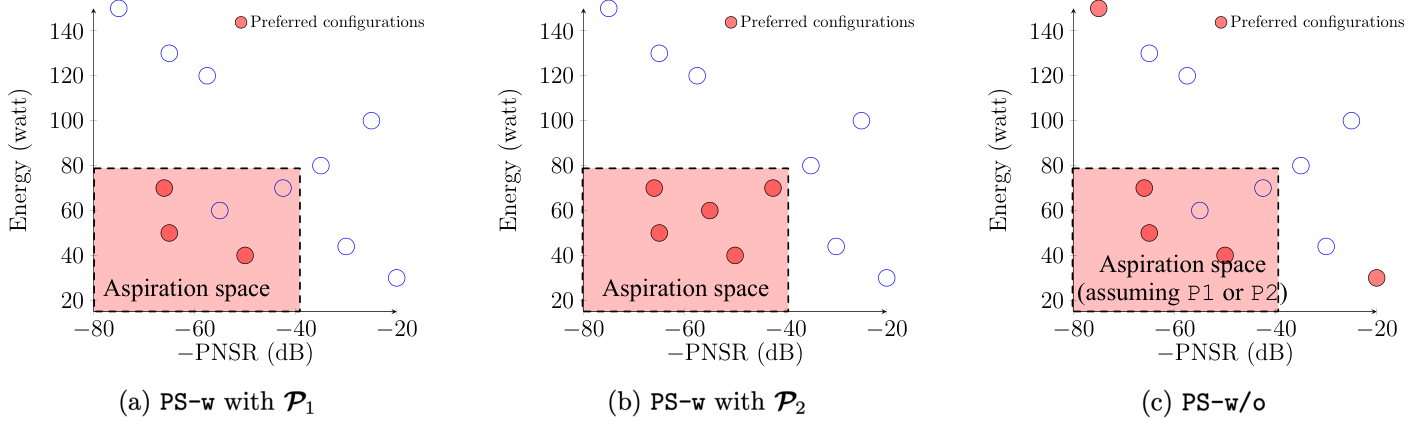
To make the meaning of the above clear for PS-w and PS-w/o, Figure 3 illustrates what configurations are preferred when using PS-w and PS-w/o in the tuning under $\mathbfcal{P}_{1}$ or $\mathbfcal{P}_{2}$ . Here, the quality of the configurations produced would need to be evaluated with respect to the requirements and PS-w prefers precisely what is needed therein. PS-w/o, in contrast, naturally prefers all configurations on the Pareto front. Intuitively, we note that PS-w/o would also prefer some configurations that are preferred by its PS-w counterpart. For example, when comparing Figure 3a and 3c, all the points preferred by PS-w are also preferred by PS-w/o (but not vice versus), hence they should converge to the same satisfiability under $\mathbfcal{P}_{1}$ . In Figure 3b and 3c, although PS-w/o prefers different points to that of PS-w in the aspiration space, they should be able to reach the same degree of satisfaction with respect to the requirements because all configurations within the aspiration space are deemed equivalent when being evaluated by $\mathbfcal{P}_{2}$ . Indeed, if both PS-w and PS-w/o can find all their preferred points in the space, then the engineers can simply cherry-pick the fully satisfied ones according to the given performance requirements from the final set of configurations returned. Yet, the unanswered question would be: is the above assumption true and hence there would be no difference regarding whether PS-w or PS-w/o is chosen?

The rest of this paper provides an empirical understanding of the above confusion.

3. How Requirements are Handled

Here we describe the process of mining, classifying, and analyzing the real-world performance requirements with aspirations. We use Cohen’s Kappa coefficient ( $\kappa$ ) (McHugh 2012) to mitigate bias between authors — the classification is often regarded as unbiased and sustainable when $\kappa>0.7$ . In a nutshell, Cohen’s Kappa coefficient is generally thought to be a more robust measure than a simple percent agreement calculation between the raters, as it takes into account the possibility of the agreement occurring by chance. In this work, we use the coefficient in two aspects:

•

Measure the agreement on which implication category a requirement belongs to (we have $\kappa=0.85$ ).
•

Measure the agreement on which patterns that a paper assumes (we have $\kappa=0.76$ ).

3.1. Real-world Requirements with Aspirations

To understand what are the common real-world performance requirements with aspirations and their implications in the industry, in Jan 2021, we mined the publicly available requirement dataset from Zenodo (under the Empirical Software Engineering label), GitHub, and the Google Dataset Search, using a keyword “requirement dataset”, as shown in Figure 4. The results led to 386 items, including duplication and many irrelevant ones which can be easily identified from their titles. As such, we filtered the candidates down to 14, within which we followed the criteria below to extract the most relevant ones for this study:

•

The dataset has clearly documented requirement statements for the software systems to be built.
•

The dataset contains labeled requirements for performance objectives or there is readily available code to do so.
•

To ensure external validity, the dataset contains performance requirements for systems from different domains.

The process has resulted in nine shortlisted datasets, based on which we attempted to identify the statements of performance requirements according to the following rules:

•

The performance requirement should contain a quantifiable aspiration level, such as “the system shall perform with 1500 users at a time”. In contrast, “the system shall be fast” is too vague to be quantified.
•

To ensure fairness when comparing with the PS-w/o, we eliminate the performance requirements that do not prefer one extreme of the objective, such as “the display shall be refreshed every 60 seconds”. This is because such requirements prefer the performance to reach a clear aspiration (e.g., 60 seconds) instead of a maximum/minimum of the performance objective. Therefore, in such a case, PS-w should always be preferred, since there is no point to use PS-w/o which naturally maximizes/minimizes the objectives while does not take aspiration into account⁶⁶ 6 Note that, indeed, in some cases, the preference of this kind of requirement can be derived by inferring from the context. Using the same example, if the display could not be refreshed because some long-running analyses could not be terminated within 60 seconds, then the preference would be to guarantee the ability to refresh every 60-sec or less. However, in our cases, most of those requirements come from the PROMISE dataset, which has no extra information other than some sentences describing the requirement. This makes it difficult for us to correctly infer the preferences implied. Hence, in the above example, we stick with the literal meaning that one would prefer and only prefer a refresh rate of 60 seconds; no more and no less..

The above has led us to rule out four datasets that contain no appropriate requirements. Table 1 shows details of the final five datasets used in our study (removing duplication).

Table 1. Performance requirements with aspirations.

Dataset	# Requirements	Link
Do et al. (Do et al. 2019)	52	https://github.com/aqd14/ICSR-2019
PROMISE (Menzies et al. 2012)	48	https://zenodo.org/record/268542
PURE (Ferrari et al. 2017)	28	https://zenodo.org/record/1414117
Shaukat et al. (Shaukat et al. 2018)	13	https://zenodo.org/record/1209601
Dalpiaz et al. (Dalpiaz et al. 2019)	10	https://zenodo.org/record/3309669

3.2. Literature Search of Patterns

As from Figure 4, we also conducted a literature search according to the best practice of a systematic literature review in software engineering (Kitchenham et al. 2009), containing search protocol, inclusion, and exclusion criteria. Our goal is to understand a single question: how are the implications of real-world performance requirements with aspirations, which are generic to the software systems as identified from Section 3.1, have been specifically quantified in current bi-objective software configuration tuning work? Note that we do not intend to be comprehensive, but rather to gather representatives.

In Feb 2021, we conducted a full-text search over Google Scholar for papers published since 2010 from the software engineering community (we exclude the system-related papers for better representation in the community), using a focused search string below:

“requirement” AND (“multi objective” OR “multi goal” OR “multi criteria”) AND (“performance” OR “non-functional”) AND (“configurable software” OR “adaptive software”) AND (“tuning” OR “optimization”)

This gives us 426 papers. We then filtered patents, inaccessible papers, and any non-English documents, leading to 393 papers. Next, we further extracted the papers by using the following inclusion criteria on the title and abstract:

•

The paper is relevant to tuning the configuration of the software system.
•

The paper seeks to improve or evaluate the performance objectives of the software system.
•

The paper considers performance requirements.
•

The paper is peer-reviewed and is not a survey or tutorial.

A paper was ruled out if it does not meet all the above criteria, which resulted in 107 papers. Then, we removed papers based on the following exclusion criteria by reviewing the content:

•

The considered performance requirements do not have a clear aspiration level.
•

The paper tackle only a single performance objective.
•

The paper does not have quantitatively experimental results with clear instructions on how the results were obtained.

A paper was ruled out if it met any of the above criteria. Finally, we obtained 29 papers, as shown in Table 2.

Table 2. Identified papers with aspiration quantification.

Venue	# Papers	Venue	# Papers	Venue	# Papers
TSE (journal)	3	JSS (journal)	6	TAAS (journal)	3
ASE (journal)	2	ESE (journal)	1	ICPE (conference)	1
ICSE (conference)	1	FSE (conference)	3	ASE (conference)	1
SEAMS (symposium)	6	ICSA (conference)	1	MODELS (conference)	1

3.3. Results Analysis

3.3.1. Number of Performance Objectives

From the review, we found that 26 out of 29 (90%) of the papers considered two performance objectives in their tuning process. The remaining three papers take into account three or more. This is a clear sign that two performance objectives remain a state-of-the-art setting for tuning software configuration, which is consistent with the finding from the recent survey for a related field (Chen et al. 2020). Therefore, in this work, we focus on bi-objective software configuration tuning.

3.3.2. Implications

We analyzed all 151 performance requirements with aspirations from Section 3.1, and found three possible implications on the aspiration space for a given performance objective:

•

$\mathbf{\mathcal{I}_{1}}$ : Anything in the aspiration space is equally preferred. This gives a clear upper aspiration bound without other information, e.g., “the server will support a maximum of 1,000 simultaneous users”; or there is a lower aspiration bound but clear information has been given for the cases when the performance reaches the aspiration space, e.g., “results shall be returned in under 15 seconds”.
•

$\mathbf{\mathcal{I}_{2}}$ : Anything not in the aspiration space is equally non-preferred. For example, “the system shall allow for a minimum of 6 users at the same time”, in which case there is only information for a clear lower aspiration bound.
•

$\mathbf{\mathcal{I}_{3}}$ : No information is available with respect to the aspiration space. This often refers to the requirements where there is a clear aspiration level, but no indication about whether it is an upper or lower aspiration bound while any other information is unavailable. For example “the system shall cater to 10 simultaneous users”.

The distribution of the implications can be found in Figure 5(a) and we achieve a Kappa coefficient $\kappa=0.85$ for this.

(a)

\#

requirements per implication

(b)

\#

papers per pattern

Pattern	Implication
$\boldsymbol{p}_{1}$	$\mathcal{I}_{1}$ , $\mathcal{I}_{3}$
$\boldsymbol{p}_{2}$	$\mathcal{I}_{1}$ , $\mathcal{I}_{2}$ , $\mathcal{I}_{3}$
$\boldsymbol{p}_{3}$	$\mathcal{I}_{2}$ , $\mathcal{I}_{3}$

Figure 5. Distribution of implications, patterns and their mappings (six papers consider more than one pattern).

Figure 6. Requirement patterns with (and without) aspiration from the literature.

\alpha

and

\beta

denote the lower and upper bound of the performance objective, respectively.

d

is the aspiration level and the aspiration space has been shaded.

3.3.3. Patterns

Next, with the above implications in mind, we seek to understand how they are quantified within the 29 papers identified. This led to three state-of-the-art patterns on the functions to quantify requirements with aspiration level (assuming the lower bound is optimum). Suppose that $\alpha$ and $\beta$ denote the lower and upper bound of the performance objective, respectively; $d$ is the aspiration level, the patterns, and their quantification have been shown in Figure 6 and are explained below:

•

$\boldsymbol{p_{1}}$ : The performance in the aspiration space is equally good or otherwise there is a certain degree of tolerance (Figure 6b). The function can be formulated as:

(3) $\displaystyle\boldsymbol{p_{1}}(x)=\begin{cases}{{\beta-x}\over{\beta-d}}&x>d\\ 1&x\leq d\end{cases}$
•

$\boldsymbol{p_{2}}$ : The performance in the aspiration space is equally good while anything outside the space is unacceptable (Figure 6c), such that:

(4) $\displaystyle\boldsymbol{p_{2}}(x)=\begin{cases}0&x>d\\ 1&x\leq d\end{cases}$
•

$\boldsymbol{p_{3}}$ : Preferring the optimal performance while anything outside the aspiration space is unacceptable (Figure 6d), which is defined as:

(5) $\displaystyle\boldsymbol{p_{3}}(x)=\begin{cases}0&x>d\\ {{d-x}\over{d-\alpha}}&x\leq d\end{cases}$

Similarly, we can also formalize the requirement with no clear aspiration level involved (e.g., “the latency shall be small”), denoted as $\boldsymbol{p_{0}}$ , which is illustrated in Figure 6a and can be formulated as follow:

(6)

\displaystyle\boldsymbol{p_{0}}(x)={{\beta-x}\over{\beta-\alpha}}

The distribution of the patterns has been shown in Figure 5(b) where we have $\kappa=0.76$ , which is sustainable (McHugh 2012).

Through normalization in those patterns, the raw measurement of a performance objective is transformed into the satisficing degree with respect to a given aspiration space (if any), ranging between 0 and 1 where the latter means fully satisfied. As such, the transformation depends on the assumption of satisficing over measurements included or excluded by the aspiration space, which distinguishes the patterns. At this point, we can immediately see the mappings between the patterns and the extracted implications from the real-world dataset. Such mappings have been illustrated in Figure 5(c), from which we see that each pattern, except $\boldsymbol{p_{0}}$ , can fit with at least two implications from the real-world requirements. For example, $\boldsymbol{p_{1}}$ can fit with $\mathcal{I}_{1}$ and $\mathcal{I}_{3}$ , because the former prefers anything within the aspiration space and specifies nothing on the other extreme, while the latter has no information at all and thus one needs to rely on an assumption when quantifying $\mathcal{I}_{3}$ to guide the search, meaning that it has the possibility to fit with all the three patterns.

From the above, it is confirmed that there exist patterns from current work which can reflect the implication of real-world performance requirements and their aspirations. We, therefore, will seek to examine all of them in our empirical study.

Figure 7. Example of using the patterns for evaluating the goodness of configurations and guiding PS-w in the transformed space.

3.4. Respecting Requirements and Aspiration in Software Configuration Tuning

While the above requirement patterns are the key to evaluating the “better” or “worse” in the set of configurations produced by any Pareto optimizer and optimization model, they directly influence the behavior of PS-w (they correspond to the $p_{n}$ in Equation (1)) but not that of the PS-w/o.

Most importantly, those patterns allow us to precisely quantify what is the best configuration(s) amongst the configurations produced by those two optimization models given a set of requirements and aspirations. Figure 7 shows an example of evaluating the configurations (and guiding PS-w) in a transformed space when taking the requirements and aspirations into account, i.e., energy usage with $\boldsymbol{p_{1}}$ and aspiration of 80 watts while PNSR with $\boldsymbol{p_{3}}$ and aspiration of 40dB. Here, we certainly prefer the points within the aspiration space in contrast to those outside. However, for those points within the aspiration space, we only prefer those with better PNSR while the energy usage is deemed as equivalent (due to the implication of $\boldsymbol{p_{1}}$ and $\boldsymbol{p_{3}}$ ).

The above is difficult to assess and quantify in the original space (Figure 7 left), since naturally the points that are non-dominated by each other (in the sense of the original objective values) are considered as equivalent when the requirements and aspiration are not involved. Therefore, the actual most preferred point (arrow highlighted) is not considered the best. In contrast, the evaluation becomes immediately obvious on what is the best point in the transformed space, where the energy and PNSR are converted by the equations for $\boldsymbol{p_{1}}$ and $\boldsymbol{p_{3}}$ , respectively. Now, clearly, the most preferred point is the only non-dominated point therein (Figure 7 right).

4. Empirical Study Design

As shown in Figure 8, our methodology consists of the following steps:

Step 1:

Assume that a requirement scenario has been negotiated by the software engineers and stakeholders, we quantify the requirements such that they are ready for the Pareto optimizers, i.e., in the forms of a combination of patterns from Section 3 and their aspiration space. In particular, to form a requirement scenario, the given combination of the patterns is denoted as a two-dimensional vector $\mathbfcal{P}$ , such that there is at least one that comes with a clear aspiration level, e.g., $\mathbfcal{P}=\{\boldsymbol{p}_{0},\boldsymbol{p}_{3}\}$ . In this work, we examine all possible combinations of the patterns (including $\boldsymbol{p_{0}}$ ). Under each combination, we also consider different aspiration spaces for our RQs; this will be further elaborated in Section 4.2.

Figure 8. Overview of the empirical study.
Step 2:

Run both PS-w/o and PS-w on different software systems. Particularly, when formulating the performance objectives, PS-w/o is steered by the raw measurements only⁷⁷ 7 This is effectively identical to using $\boldsymbol{p_{0}}$ for all performance objectives. while PS-w is designed to be guided by the given vector of patterns $\mathbfcal{P}$ as the new objectives. To ensure fairness, both optimization models are examined under the same optimizer and we consider three representative optimizers in this work, i.e., NSGA-II (Deb et al. 2002), IBEA (Zitzler and Künzli 2004), and MOEA/D (Zhang and Li 2007).
Step 3:

Measure the system as the search proceeds until the tuning budget has been exhausted; repeat 100 times.
Step 4:

Evaluate the set of configurations thereafter using $\mathbfcal{P}$ as part of the Quality Evaluation phase.
Step 5:

Go back to Step 1 if there are more combinations of patterns and aspirations to examine.

Table 3. The considered requirement scenarios (in terms of the combination of the patterns identified from Section 3) and their example interpretations. The interpretations are based on the assumption that the performance objectives are

\{latency,throughput\}

with possible aspiration levels

d_{1}

and

d_{2}

, respectively.

Possible $\mathbfcal{P}$	Example Interpretation
$\{\boldsymbol{p_{0}},\boldsymbol{p_{1}}\}$	Prefer better latency and throughput better than $d_{2}$ , but any configurations better than $d_{2}$ are equally preferred; willing to accept throughput worse than $d_{2}$ .
$\{\boldsymbol{p_{1}},\boldsymbol{p_{0}}\}$	Prefer better throughput and latency better than $d_{1}$ , but any configurations better than $d_{1}$ are equally preferred; willing to accept latency worse than $d_{1}$ .
$\{\boldsymbol{p_{0}},\boldsymbol{p_{2}}\}$	Prefer better latency and throughput better than $d_{2}$ , but any configurations better than $d_{2}$ are equally preferred; do not accept throughput worse than $d_{2}$ .
$\{\boldsymbol{p_{2}},\boldsymbol{p_{0}}\}$	Prefer better throughput and latency better than $d_{1}$ , but any configurations better than $d_{1}$ are equally preferred; do not accept latency worse than $d_{1}$ .
$\{\boldsymbol{p_{0}},\boldsymbol{p_{3}}\}$	Prefer better latency and throughput; do not accept throughput worse than $d_{2}$ .
$\{\boldsymbol{p_{3}},\boldsymbol{p_{0}}\}$	Prefer better latency and throughput; do not accept latency worse than $d_{1}$ .
$\{\boldsymbol{p_{1}},\boldsymbol{p_{1}}\}$	Prefer latency better than $d_{1}$ and throughput better than $d_{2}$ , but any configurations better than $d_{1}$ and $d_{2}$ are equally preferred; willing to accept latency and throughput worse than $d_{1}$ and $d_{2}$ , respectively.
$\{\boldsymbol{p_{2}},\boldsymbol{p_{2}}\}$	Prefer latency better than $d_{1}$ and throughput better than $d_{2}$ , but any configurations better than $d_{1}$ and $d_{2}$ are equally preferred; do not accept latency and throughput worse than $d_{1}$ and $d_{2}$ , respectively.
$\{\boldsymbol{p_{3}},\boldsymbol{p_{3}}\}$	Prefer better latency and throughput; do not accept latency and throughput worse than $d_{1}$ and $d_{2}$ , respectively.
$\{\boldsymbol{p_{1}},\boldsymbol{p_{2}}\}$	Prefer latency better than $d_{1}$ and throughput better than $d_{2}$ , but any configurations better than $d_{1}$ and $d_{2}$ are equally preferred; willing to accept latency worse than $d_{1}$ but do not accept throughput worse than $d_{2}$ .
$\{\boldsymbol{p_{2}},\boldsymbol{p_{1}}\}$	Prefer latency better than $d_{1}$ and throughput better than $d_{2}$ , but any configurations better than $d_{1}$ and $d_{2}$ are equally preferred; willing to accept throughput worse than $d_{2}$ but do not accept latency worse than $d_{1}$ .
$\{\boldsymbol{p_{1}},\boldsymbol{p_{3}}\}$	Prefer better throughput and latency better than $d_{1}$ , but any configurations better than $d_{1}$ are equally preferred; willing to accept latency worse than $d_{1}$ but do not accept throughput worse than $d_{2}$ .
$\{\boldsymbol{p_{3}},\boldsymbol{p_{1}}\}$	Prefer better latency and throughput better than $d_{2}$ , but any configurations better than $d_{2}$ are equally preferred; willing to accept throughput worse than $d_{2}$ but do not accept latency worse than $d_{1}$ .
$\{\boldsymbol{p_{2}},\boldsymbol{p_{3}}\}$	Prefer better throughput and latency better than $d_{1}$ , but any configurations better than $d_{1}$ are equally preferred; do not accept latency worse than $d_{1}$ nor throughput worse than $d_{2}$ .
$\{\boldsymbol{p_{3}},\boldsymbol{p_{2}}\}$	Prefer better latency and throughput better than $d_{2}$ , but any configurations better than $d_{2}$ are equally preferred; do not accept latency worse than $d_{1}$ nor throughput worse than $d_{2}$ .

It is worth noting that, although the patterns from Section 3 are for single performance objective, they can be arbitrarily combined for the bi-objective software configuration tuning in the Scenario Identification phase of Step 1 (Calinescu et al. 2017; Martens et al. 2010; Gerasimou et al. 2016; Calinescu et al. 2018), as illustrated in Table 3.

In the Configuration Tuning phase (Step 2 and 3), the patterns require normalization using the lower and/or upper bound (except for $\boldsymbol{p_{0}}$ and $\boldsymbol{p_{2}}$ ). However, since these are often unknown, we adopt a dynamic method wherein the raw measurements are normalized using the maximal and minimal values found so far as the tuning proceeds, which is common in SBSE for software configuration tuning (Shahbazian et al. 2020; Bowers et al. 2018). We record the raw measurements of each configuration throughout the tuning to efficiently utilize the tuning budget (Section 4.3.2).

To mitigate stochastic bias, we repeat each experiment 100 runs. The study is conducted on a cluster of machines each with Intel i5 six cores CPU at 2.9GHz and 8GB memory, running numerous experiments in parallel over the course of five months ( $24\times 7$ ).

4.1. Subject Software Systems

We conduct our study on a set of real-world highly configurable software systems and environments that have been widely studied in existing work (Jamshidi et al. 2018; Nair et al. 2020; Jamshidi and Casale 2016; Chen and Li 2021). These are selected according to the criteria below:

(1)

To ensure that the search landscape is not too trivial to be explored, the system should contain a mix of binary and enumerative configuration options.
(2)

A full exploration of the search space is infeasible, i.e., it cannot be done within 24 hours.
(3)

There are clear instructions on how to set up the benchmark under which the system will be measured.
(4)

If the same system of an environment has been used with a different set of configuration options, choose those with relatively higher complexity, i.e., larger search space and more configuration options. For example, Storm can be tuned under different workload benchmarks, and we choose WordCount and RollingSort as the two that satisfy the above criteria.

We firstly eliminated LLVM from (Nair et al. 2020), as it violates Criterion (1). Similarly, sort-256 and noc-CM-log is also ruled out due to their rather small search space which can be exhaustively explored in 24 hours, i.e., Criterion (2). We cannot consider the system SaC as there is no clear instruction on under what benchmark it can be profiled, which violates Criterion (3). We also noticed that Storm and Keras (with DNN or LSTM) have been much more commonly used than others, but with different configuration options and environments. Therefore, according to Criterion (4), we use the settings that lead to a much larger search space and more options. As shown in Table 4, the selected software systems come from diverse domains, e.g., video encoding, stream processing, and deep/machine learning, while having different performance objectives, scales, and search spaces. Their measurements are also expensive⁸⁸ 8 Each measurement consists of 5 repeated samples and the median value is used., e.g., XGBoost needs 2,807 hours to explore less than 1% of its search space.

We keep the same performance objectives, configuration options, and their ranges as studied in the prior work that made use of them, e.g., (Jamshidi et al. 2018; Nair et al. 2020; Jamshidi and Casale 2016; Chen and Li 2021), since those have been shown to be the key ones for the software systems under the related environment. As a result, although the software systems are the same, the actual search spaces are different, such as Storm/WC and Storm/RS. In particular, following what has been used in previous work, the environment/workload we consider are:

Table 4. Configurable software systems studied. We run all software systems under their standard benchmarks. Storm and Keras (with DNN) use two benchmarks and three dataset, respectively.

Software	Domain	Performance Objectives	$\#$ Options	Search Space	Used By
Trimesh	Mesh solver	Latency and $\#$ Iteration	13	239,260	(Nair et al. 2020; Chen and Li 2021)
x264	Video encoding	PSNR and Energy Usage	17	53,662	(Nair et al. 2020; Chen and Li 2021)
Storm/WC	Stream processing	Latency and Throughput	6	2,880	(Nair et al. 2020; Chen and Li 2021; Jamshidi and Casale 2016; Jamshidi et al. 2018)
Storm/RS	Stream processing	Latency and Throughput	6	3,839	(Nair et al. 2020; Chen and Li 2021; Jamshidi and Casale 2016; Jamshidi et al. 2018)
Keras/Adiac	Deep learning	AUC and Inference Time	13	3.99 $\times 10^{13}$	(Jamshidi et al. 2018)
Keras/DSR	Deep learning	AUC and Inference Time	13	3.32 $\times 10^{13}$	(Jamshidi et al. 2018; Chen and Li 2021)
Keras/SA	Deep learning	AUC and Inference Time	13	2.66 $\times 10^{13}$	(Jamshidi et al. 2018)
XGBoost	Machine learning	Accuracy and Training Time	13	2.88 $\times 10^{10}$	(Jamshidi et al. 2018)

•

Trimesh: we use the Shapenet dataset that contains 51,300 unique 3D models. In this work, we randomly sample 100 models as the standard benchmark.
•

x264: for this, the benchmark used is a standard video of 1GB size, which was chosen randomly.
•

Storm/WC: we use the WordCount as the benchmark. This is a typical simple streaming example where Storm is used to keep track of the words and their counts streaming in. WordCount generates a CPU-intensive workload.
•

Storm/RS: similar to Storm/WC, here we use the RollingSort as the benchmark. Unlike WordCount, RollingSort generates a memory intensive workload.
•

Keras/Adiac: we use the Deep Neural Network (DNN) from the Keras software and run it on the Adiac dataset. Generally, the dataset contains a task of automatic identification of diatoms (unicellular algae) among 31 classes with a training and testing size of 390 and 391, respectively.
•

Keras/DSR: we use the DNN from the Keras software and run it on the DiatomSizeReduction dataset. The dataset concerns the prediction of four types of diatoms with a training and testing size of 16 and 306, respectively.
•

Keras/SA: we use the DNN from the Keras software and run it on the ShapesAll dataset. Generally, the dataset aims to test contour/image and skeleton-based descriptors; there are 60 classes with a training and testing size of 600 each.
•

XGBoost: we use the Covertype dataset that contains 54 forest cover type from cartographic variables only. The size of the dataset is 581,012 and we follow a 70%-30% training and testing split.

Indeed, the analyzed dataset and literature in Section 3 may not specifically target the software systems considered in this work. However, the extracted implication and patterns are rather generic such that they can be applied to different cases. Further, some widely studied performance objectives (from both the dataset and literature) are overwhelmingly applicable. For example, latency- and throughput-related requirements (with different aspiration levels) are prevalent for a wide range of software (Nair et al. 2020).

Table 5. Aspiration levels and spaces for the configurable software systems studied (used for all combinations of patterns).

l

r

c

, and

u

denote left-shifted, right-shifted, centered, and unrealistic aspirations, respectively.

Software	Performance Objectives	$l$	$r$	$c$	$u$
Trimesh	$\{$ Latency (s), # Iterations $\}$	$\{81,4\}$	$\{461,15\}$	$\{135,7\}$	$\{37,501\}$
x264	$\{$ PSNR (dB), Energy Usage (W) $\}$	$\{50,3680\}$	$\{37,462\}$	$\{46,1260\}$	$\{100,34\}$
Storm/WC	$\{$ Throughput (msgs/m), Latency (ms) $\}$	$\{16473,15677\}$	$\{994,5\}$	$\{8982,101\}$	$\{34740,3\}$
Storm/RS	$\{$ Throughput (msgs/m), Latency (ms) $\}$	$\{1.3\times 10^{5},7819\}$	$\{3006,5\}$	$\{3.7\times 10^{4},126\}$	$\{2.3\times 10^{5},1.9\}$
Keras/Adiac	$\{$ AUC, Inference Time (ms) $\}$	$\{0.030,44\}$	$\{0.017,0.05\}$	$\{0.028,3\}$	$\{0.292,0.03\}$
Keras/DSR	$\{$ AUC, Inference Time (ms) $\}$	$\{0.307,123\}$	$\{0.107,0.12\}$	$\{0.300,25\}$	$\{0.581,0.031\}$
Keras/SA	$\{$ AUC, Inference Time (ms) $\}$	$\{0.167,21\}$	$\{0.157,0.07\}$	$\{0.160,6\}$	$\{0.325,0.04\}$
XGBoost	$\{$ Accuracy (%), Training Time (s) $\}$	$\{80,42\}$	$\{54,3\}$	$\{72,8\}$	$\{92,1\}$

4.2. Aspiration Space

To improve external validity, we consider aspiration levels that draw two types of aspiration space under two performance objectives: realistic and unrealistic ones. To that end, for each software system, we run all the Pareto optimizers for three hours each to obtain a landscape that contains an approximated Pareto front. We do so by ensuring that the obtained front is reasonably converged, i.e., increasing the budget only marginally changes the results. We then set the aspiration space based on such a front as summarized in Table 5.

4.2.1. Realistic Aspiration Space

For software configuration tuning with two performance objectives, we say an aspiration space is realistic if there is at least one configuration that can reach the aspiration levels of both performance objectives.

Using Storm/RS as an example in Figure 9, for the realistic ones under each combination of patterns, we set three aspiration space based on their positions in the objective space: left-shifted ( $l$ ), right-shifted ( $r$ ) and centered ( $c$ ). In particular, $l$ is defined as using the value of the 20 $th$ percentile for throughput and the value of the 80 $th$ percentile for latency as their corresponding aspiration levels; similarly, $r$ uses the value of the 20 $th$ percentile for latency and the value of the 80 $th$ percentile for throughput; finally, $c$ uses the values of the 50 $th$ percentile for both performance objectives. Clearly, despite covering diverse regions in the overall space of performance objectives, all those spaces contain at least one point (configuration). Note that the aspiration space is applicable to any combination of patterns with and without $\boldsymbol{p_{0}}$ (in Figure 9a and Figure 9b respectively), as long as there is a clear aspiration level for at least one performance objective.

4.2.2. Unrealistic Aspiration Space

Since the aspiration level/space is negotiated beforehand, it may be unrealistic. In this work, we refer to an unrealistic aspiration space as the situation wherein the aspiration levels of two performance objectives can be at most reached one at a time, but not both simultaneously. For example, in the case of two performance objectives from Figure 9a, $u$ is an unrealistic aspiration space such that the level is achievable for either of the two objectives individually (as indicated by the dashed lines), but not for both, as there is no point (configuration) residing in the space. As a result, it is not applicable when only one performance objective contains clear aspiration, e.g., in Figure 9b. To define such a space, we set the value of 5 $th$ percentile of both performance objectives as the corresponding aspiration levels, which we have found as sufficient to create an unrealistic aspiration space for each system.

4.3. Tuning Settings

4.3.1. Pareto Optimizer

We consider three Pareto optimizers, i.e., NSGA-II (Deb et al. 2002), IBEA (Zitzler and Künzli 2004), and MOEA/D (Zhang and Li 2007), because:

•

They have been widely used for software configuration tuning in prior work (Singh et al. 2016; Calinescu et al. 2017; Martens et al. 2010; Gerasimou et al. 2016; Calinescu et al. 2018; Chen et al. 2018b).
•

They are the representatives of three fundamentally different frameworks for Pareto search (Emmerich and Deutz 2018).
•

They can, but do not have to, rely on a surrogate model(s) (Chen et al. 2018b), which greatly reduces the noise in our empirical study.

All the above optimizers are adopted for both PS-w and PS-w/o based on the implementations in jMetal (Durillo and Nebro 2011).

4.3.2. Tuning Budget

In this work, we set a budget of one hour for each run as commonly used for expensive SBSE problems (Li et al. 2020b). However, directly relying on the time as a termination criterion can suffer severe interference during the tuning as numerous experiments need to be run in parallel. To prevent this, for each software system, we did the following to convert the one-hour tuning budget into the number of unique measurements:

(1)

incrementally (100 each step) measuring distinct configurations on a dedicated machine using random sampling until the one-hour time budget is exhausted.
(2)

repeating the above 5 times and collect the number of measurements.
(3)

the median of the 5 repeats serves as the key termination criterion of the tuning thereafter (in Table 6).

Note that in each run of the tuning, we cached the measurement of every distinct configuration for direct reuse. Hence, only the distinct configurations would consume the budget.

Table 6. Population size and measurement tuning budget.

Software	Population Size	# Measurements	Software	Population Size	# Measurements
Trimesh	10	500	x264	50	1,500
Storm/WC	50	500	Storm/RS	30	700
Keras/Adiac	50	700	Keras/DSR	60	500
Keras/SA	60	500	XGBoost	30	300

4.3.3. Parameters

For the three optimizers in all cases, we apply the binary tournament, boundary mutation, and uniformed crossover, as used in prior work (Chen et al. 2018b; Chen et al. 2019). The mutation and crossover rates are set to 0.1 and 0.9, respectively, which also follows the most common setting for software configuration tuning (Chen et al. 2018b; Chen et al. 2019). Other specific settings for IBEA and MOEA/D are kept as default values, which have been shown to be effective (Chen et al. 2018b).

For each system, we pragmatically set the population size via:

(1)

examining different sizes in pilot runs under the budget in Table 6, i.e., $\{10,20,...,$ $100\}$ , over all optimizers, combinations of patterns and aspiration (on both PS-w and PS-w/o).
(2)

recording the average change rate of population over the last 10% generations using $g={1\over k}\times\sum^{k}_{i=0}{c_{i}\over s}$ , where $k$ is the number of the last 10% generations; $c_{i}$ denotes the number of different configurations in the ith generation compared with those in the i-1th generation; $s$ is the population size.
(3)

the largest population size where $g\leq 0.1$ across all conditions (or 10, if no size satisfies the above constraints) will be used.

The results are also shown in Table 6. In this way, we seek to reach a balance between convergence (smaller population change) and diversity (larger population size) under the given tuning budget. That is, increasing the budget will unlikely change the result. This has been practiced in (Gerasimou et al. 2018; Chen and Li 2021).

4.4. Analysis and Comparison

4.4.1. Metric

To make a comparison and determine which optimization model is better in this work, we need to measure the “best” with two conditions in mind:

•

Condition 1: The metric needs to be able to comprehensively compare the different sets of configurations as produced by the Pareto optimizers, covering diverse quality aspects, such as convergence and diversity.
•

Condition 2: The metric should be able to reflect the given requirement scenarios, i.e., taking the given patterns identified from Section 3 into account when conducting the comparisons and evaluations.

To that end, we use Hypervolume (HV) (Zitzler and Thiele 1998; Zitzler et al. 2007) as the basic metric to assess the quality of the configuration set produced in each run. In a nutshell, HV measures the volume between all points of a configuration set and a reference point (usually a nadir point); the larger the volume, the better convergence, and diversity that the set achieves. HV is chosen in this work because:

•

HV is a comprehensive metric that covers all quality aspects of a configuration set, i.e., convergence, uniformity, spread, and cardinality (Li and Yao 2019; Li et al. 2022), which meets Condition 1.
•

HV also does not require a reference Pareto front and is Pareto compliant⁹⁹ 9 Generally speaking, a quality indicator being Pareto compliant means that its evaluation result does not conflict with the Pareto dominance relation between two solution sets. More strictly, if a solution set $A$ is better (Zitzler et al. 2003) than $B$ (i.e., for any solution in $B$ , there exists one solution in $A$ that covers (dominates or is equivalent to) it, and there exists at least one solution in $A$ that is not covered by any solution in $B$ ), then $A$ is always evaluated better than $B$ by the indicator., which fits our case as the true Pareto front is unknown.
•

By following the guidelines proposed by (Li et al. 2018; Li et al. 2022), we landed on HV as the appropriate metric for our SBSE problem.

(a) Evaluating with HV in the original space

(b) Evaluating with HV in the transformed space

Figure 10. Evaluation of HV with and without requirements/aspirations.

Since we are interested in a requirement scenario that has a specific combination of patterns and aspiration space ( $\mathbfcal{P}$ ) in the objective space, the original HV, which always favors the configurations that are close to the entire Pareto front, is no longer suitable. Therefore, we need to transfer these preferences into the HV following the guidance by Li et al. (Li et al. 2022) and leveraging the patterns and quantification from Section 3 (for satisfying Condition 2). Using the same example from Section 2.2, as shown in Figure 10, the requirement scenario is that: the stakeholders prefer better PNSR and energy usage better than 80 watts, but any configurations better than 80 watts are equally preferred; willing to accept energy usage worse than 80 watts but do not accept PNSR worse than 40dB. This means for any points in the aspiration space, the ones with better PNSR would be preferred more. Therefore, point $\boldsymbol{A}$ is the best based on the requirements and should contribute the most to the chosen metric. However, directly applying HV would make some configurations, which are less preferred to the requirements, contribute significantly to the HV value (Figure 10a). This would misleadingly evaluate some sets that have many non-preferred points to have a very good HV value. In contrast, when transferring the information of patterns before using HV (i.e., in the transformed space), the above requirements and aspirations can be better complied with, as $\boldsymbol{A}$ is certainly the one that contributes the most and other non-preferred points tend to have no or little contributions. (Figure 10b)

To that end, we extend the HV in this work. Suppose that there are $m$ performance objectives (we have $m=2$ in this work) and $\mathbfcal{A}$ is a produced configuration set wherein the vector of a configuration’s raw measurements is $\boldsymbol{\overline{x}_{i}}=\{x_{1},x_{2},...x_{m}\}$ , we calculate HV based on the converted satisficing value of $\boldsymbol{\overline{x}_{i}}$ according to the given $\mathbfcal{P}$ . We call it aspiration-aware HV (dubbed A-HV), which is formulated as:

(7)

A\mathchar 45\relax HV(\mathbfcal{A})=\lambda(\bigcup_{\boldsymbol{\overline{x}_{i}}\in\mathbfcal{A}}\{\boldsymbol{v}|\mathbfcal{P}(\boldsymbol{\overline{x}_{i}})\prec\boldsymbol{v}\prec\boldsymbol{r}\})

where $\lambda$ is the Lebesgue measure that quantifies the volume (Zitzler and Thiele 1998) as used in the original HV; $\boldsymbol{r}$ is the reference nadir point, which is often taken as the 1.1 times of the range of the nondominated set (Li et al. 2022), hence in our case, this would be $\{-0.1,-0.1\}$ as $\mathbfcal{P}(\boldsymbol{\overline{x}_{i}})$ converts the outputs to $[0,1]$ . Like HV, a higher A-HV value is better. To ensure fair comparison with A-HV, we use the minimum and/or maximum values (of each performance objective) from all experiments for the posterior normalization in the patterns.

To enable more intuitive exposition, we report on the % gain of the A-HV for considering requirements and aspirations in the tuning, i.e., PS-w, over that for PS-w/o on each run, which is defined as:

(8)

\text{\% Gain}={{{x_{i}-y_{i}}\over{y_{i}}}}\times 100

whereby $x_{i}$ and $y_{i}$ are the A-HV value at the $i$ th run for PS-w and PS-w/o, respectively, in their sorted lists. Clearly, a positive % gain indicates that the aspirations are helpful (PS-w is better) while a negative value implies they are harmful (PS-w/o is better); zero gain means identical result.

4.4.2. Statistical Validation

We use the standard methods to interpret the significance of the results over 100 runs in each case (Arcuri and Briand 2011; Kampenes et al. 2007):

•

Wilcoxon test: We apply the Wilcoxon test (Wilcoxon 1945) with $a=0.05$ (Arcuri and Briand 2011) to investigate the statistical significance of the A-HV comparisons over all 100 runs, as it is a non-parametric statistical test that makes little assumption about the data distribution and has been recommended in software engineering research for pair-wise comparisons (Arcuri and Briand 2011).
•

$\mathbf{\hat{A}_{12}}$ effect size: To ensure that a $p<0.05$ is not caused by a trivial amount of the samples, we apply $\hat{A}_{12}$ (Vargha and Delaney 2000) to measure the effect size. In this work, $\hat{A}_{12}>0.5$ denotes PS-w wins wherein it has better A-HV for more than 50% of the runs. $\hat{A}_{12}\geq 0.6$ or $\hat{A}_{12}\leq 0.4$ indicate a non-trivial effect size. Since there are 100 runs (instead of the commonly used 30), we use a stricter interpretation by which $0.6\leq\hat{A}_{12}<0.7$ (0.3 < $\hat{A}_{12}\leq 0.4$ ), $0.7\leq\hat{A}_{12}<0.8$ (0.2 < $\hat{A}_{12}\leq 0.3$ ), and $\hat{A}_{12}\geq 0.8$ ( $\hat{A}_{12}\leq 0.2$ ) indicate small, medium, and large effect, respectively.

5. Results and Findings

In this section, we present the results of our empirical study and address the research questions posed in Section 1.

5.1. RQ1: Which is Better under Requirements with Realistic Aspirations?

5.1.1. Method

To answer RQ1, we compare PS-w and PS-w/o across 15 combinations of patterns, three realistic aspiration spaces ( $l$ , $r$ , and $c$ ), three optimizers and eight subject systems, leading to $15\times 3\times 3\times 8=1,080$ cases. Since we are interested in a pair-wise comparison of the A-HV under each case, the Wilcoxon test and $\hat{A}_{12}$ are used to verify the statistical significance over 100 runs.

5.1.2. Results

As an overview, Figure 11 shows a summary of the $\hat{A}_{12}$ outcomes across the cases. Clearly, we see that PS-w performs overwhelmingly better than its PS-w/o counterpart. In particular, PS-w wins for 61% (657/1080) of the cases and loses for 16% (175/1080), while there is a 23% (248/1080) tie. In other words, PS-w is better or similar for 84% (905/1080) of the cases in contrast to the 39% (423/1080) when using PS-w/o. Statistically, PS-w wins 572 cases with $\hat{A}_{12}\geq 0.6$ and $p<0.05$ , while there are only 127 significant cases when it loses.

Table 7. Comparing PS-w and PS-w/o under realistic requirements and aspirations over 100 runs. {adjustbox}max width=.1 and {adjustbox}max width=.1 denote the average (Avg) and standard error (SE) of the positive and negative % gain, respectively. {adjustbox}max width=.1 means zero gain overall. The column “PS-w” and “PS-w/o” show the number of cases that the corresponding optimization model wins. 9 (6) means one wins on 9 cases within which 6 shows statistical significance, i.e.,

\hat{A}_{12}\geq 0.6

(or

\hat{A}_{12}\leq 0.4

) and

p<0.05

(each combination of requirement patterns has 9 cases in total, as there are 3 aspiration space and 3 optimizers). The blue cells denote PS-w wins more while red cells mean it loses more.

{adjustbox}

max width = 1

	PS-w	PS-w/o	Tie	Avg (SE) of A-HV Gain
${\{\boldsymbol{p_{0}}\textit{,}\boldsymbol{p_{1}}\}}$	8 (7)	1 (1)	0	1.1% (0.3%)	{adjustbox}max width=.1
${\{\boldsymbol{p_{1}}\textit{,}\boldsymbol{p_{0}}\}}$	7 (7)	2 (2)	0	-4.6% (1.4%)	{adjustbox}max width=.1
${\{\boldsymbol{p_{0}}\textit{,}\boldsymbol{p_{2}}\}}$	5 (5)	4 (4)	0	36.4% (10.4%)	{adjustbox}max width=.1
${\{\boldsymbol{p_{2}}\textit{,}\boldsymbol{p_{0}}\}}$	7 (7)	2 (2)	0	-3.5% (2.4%)	{adjustbox}max width=.1
${\{\boldsymbol{p_{0}}\textit{,}\boldsymbol{p_{3}}\}}$	6 (5)	3 (2)	0	29.0% (7.2%)	{adjustbox}max width=.1
${\{\boldsymbol{p_{3}}\textit{,}\boldsymbol{p_{0}}\}}$	8 (8)	1 (1)	0	2.9% (0.6%)	{adjustbox}max width=.1
${\{\boldsymbol{p_{1}}\textit{,}\boldsymbol{p_{1}}\}}$	3 (0)	2 (1)	4	-4.6% (1.4%)	{adjustbox}max width=.1
${\{\boldsymbol{p_{2}}\textit{,}\boldsymbol{p_{2}}\}}$	1 (0)	5 (1)	3	-7.6% (5.1%)	{adjustbox}max width=.1
${\{\boldsymbol{p_{3}}\textit{,}\boldsymbol{p_{3}}\}}$	6 (5)	3 (3)	0	17.8% (7.0%)	{adjustbox}max width=.1
${\{\boldsymbol{p_{1}}\textit{,}\boldsymbol{p_{2}}\}}$	3 (0)	3 (1)	3	-3.5% (5.2%)	{adjustbox}max width=.1
${\{\boldsymbol{p_{2}}\textit{,}\boldsymbol{p_{1}}\}}$	2 (0)	4 (1)	3	-6.2% (1.6%)	{adjustbox}max width=.1
${\{\boldsymbol{p_{1}}\textit{,}\boldsymbol{p_{3}}\}}$	6 (6)	3 (3)	0	6.0% (5.2%)	{adjustbox}max width=.1
${\{\boldsymbol{p_{3}}\textit{,}\boldsymbol{p_{1}}\}}$	9 (9)	0 (0)	0	3.1% (1.3%)	{adjustbox}max width=.1
${\{\boldsymbol{p_{2}}\textit{,}\boldsymbol{p_{3}}\}}$	6 (6)	3 (3)	0	-1.4% (5.9%)	{adjustbox}max width=.1
${\{\boldsymbol{p_{3}}\textit{,}\boldsymbol{p_{2}}\}}$	4 (4)	5 (3)	0	28.1% (8.2%)	{adjustbox}max width=.1

	PS-w	PS-w/o	Tie	Avg (SE) of A-HV Gain
${\{\boldsymbol{p_{0}}\textit{,}\boldsymbol{p_{1}}\}}$	9 (9)	0 (0)	0	0.2% (0.0%)	{adjustbox}max width=.1
${\{\boldsymbol{p_{1}}\textit{,}\boldsymbol{p_{0}}\}}$	6 (6)	2 (2)	1	0.1% (0.0%)	{adjustbox}max width=.1
${\{\boldsymbol{p_{0}}\textit{,}\boldsymbol{p_{2}}\}}$	8 (6)	1 (1)	0	4.9% (4.2%)	{adjustbox}max width=.1
${\{\boldsymbol{p_{2}}\textit{,}\boldsymbol{p_{0}}\}}$	6 (5)	3 (3)	0	0.1% (0.0%)	{adjustbox}max width=.1
${\{\boldsymbol{p_{0}}\textit{,}\boldsymbol{p_{3}}\}}$	3 (2)	6 (4)	0	7.2% (2.1%)	{adjustbox}max width=.1
${\{\boldsymbol{p_{3}}\textit{,}\boldsymbol{p_{0}}\}}$	6 (6)	3 (3)	0	2.1% (0.3%)	{adjustbox}max width=.1
${\{\boldsymbol{p_{1}}\textit{,}\boldsymbol{p_{1}}\}}$	1 (0)	0 (0)	8	0.1% (0.0%)	{adjustbox}max width=.1
${\{\boldsymbol{p_{2}}\textit{,}\boldsymbol{p_{2}}\}}$	1 (0)	0 (0)	8	5.0% (4.5%)	{adjustbox}max width=.1
${\{\boldsymbol{p_{3}}\textit{,}\boldsymbol{p_{3}}\}}$	3 (3)	6 (6)	0	3.6% (1.1%)	{adjustbox}max width=.1
${\{\boldsymbol{p_{1}}\textit{,}\boldsymbol{p_{2}}\}}$	1 (0)	0 (0)	8	5.0% (4.5%)	{adjustbox}max width=.1
${\{\boldsymbol{p_{2}}\textit{,}\boldsymbol{p_{1}}\}}$	1 (0)	0 (0)	8	0.1% (0.0%)	{adjustbox}max width=.1
${\{\boldsymbol{p_{1}}\textit{,}\boldsymbol{p_{3}}\}}$	5 (5)	4 (3)	0	10.0% (2.8%)	{adjustbox}max width=.1
${\{\boldsymbol{p_{3}}\textit{,}\boldsymbol{p_{1}}\}}$	9 (9)	0 (0)	0	2.8% (0.3%)	{adjustbox}max width=.1
${\{\boldsymbol{p_{2}}\textit{,}\boldsymbol{p_{3}}\}}$	6 (6)	3 (3)	0	9.3% (2.8%)	{adjustbox}max width=.1
${\{\boldsymbol{p_{3}}\textit{,}\boldsymbol{p_{2}}\}}$	8 (6)	1 (1)	0	6.3% (3.5%)	{adjustbox}max width=.1

	PS-w	PS-w/o	Tie	Avg (SE) of A-HV Gain
${\{\boldsymbol{p_{0}}\textit{,}\boldsymbol{p_{1}}\}}$	8 (8)	1 (1)	0	0.1% (0.0%)	{adjustbox}max width=.1
${\{\boldsymbol{p_{1}}\textit{,}\boldsymbol{p_{0}}\}}$	8 (8)	1 (1)	0	0.1% (0.0%)	{adjustbox}max width=.1
${\{\boldsymbol{p_{0}}\textit{,}\boldsymbol{p_{2}}\}}$	8 (8)	0 (0)	1	82.6% (17.2%)	{adjustbox}max width=.1
${\{\boldsymbol{p_{2}}\textit{,}\boldsymbol{p_{0}}\}}$	6 (6)	3 (3)	0	-0.1% (0.0%)	{adjustbox}max width=.1
${\{\boldsymbol{p_{0}}\textit{,}\boldsymbol{p_{3}}\}}$	7 (6)	2 (1)	0	90.4% (17.4%)	{adjustbox}max width=.1
${\{\boldsymbol{p_{3}}\textit{,}\boldsymbol{p_{0}}\}}$	9 (9)	0 (0)	0	67.4% (13.4%)	{adjustbox}max width=.1
${\{\boldsymbol{p_{1}}\textit{,}\boldsymbol{p_{1}}\}}$	1 (1)	0 (0)	8	0.1% (0.0%)	{adjustbox}max width=.1
${\{\boldsymbol{p_{2}}\textit{,}\boldsymbol{p_{2}}\}}$	1 (1)	0 (0)	8	83.0% (17.4%)	{adjustbox}max width=.1
${\{\boldsymbol{p_{3}}\textit{,}\boldsymbol{p_{3}}\}}$	9 (8)	0 (0)	0	142.1% (18.8%)	{adjustbox}max width=.1
${\{\boldsymbol{p_{1}}\textit{,}\boldsymbol{p_{2}}\}}$	1 (1)	0 (0)	8	83.0% (17.4%)	{adjustbox}max width=.1
${\{\boldsymbol{p_{2}}\textit{,}\boldsymbol{p_{1}}\}}$	1 (1)	0 (0)	8	0.1% (0.0%)	{adjustbox}max width=.1
${\{\boldsymbol{p_{1}}\textit{,}\boldsymbol{p_{3}}\}}$	7 (7)	2 (2)	0	91.5% (17.6%)	{adjustbox}max width=.1
${\{\boldsymbol{p_{3}}\textit{,}\boldsymbol{p_{1}}\}}$	9 (9)	0 (0)	0	67.9% (13.4%)	{adjustbox}max width=.1
${\{\boldsymbol{p_{2}}\textit{,}\boldsymbol{p_{3}}\}}$	6 (6)	3 (3)	0	91.5% (17.6%)	{adjustbox}max width=.1
${\{\boldsymbol{p_{3}}\textit{,}\boldsymbol{p_{2}}\}}$	8 (8)	1 (0)	0	142.9% (19.6%)	{adjustbox}max width=.1

(a). Trimesh

(b). x264

(c). Storm/WC

	PS-w	PS-w/o	Tie	Avg (SE) of A-HV Gain
${\{\boldsymbol{p_{0}}\textit{,}\boldsymbol{p_{1}}\}}$	8 (8)	1 (1)	0	0.1% (0.0%)	{adjustbox}max width=.1
${\{\boldsymbol{p_{1}}\textit{,}\boldsymbol{p_{0}}\}}$	6 (5)	3 (2)	0	-0.1% (0.0%)	{adjustbox}max width=.1
${\{\boldsymbol{p_{0}}\textit{,}\boldsymbol{p_{2}}\}}$	8 (7)	1 (1)	0	1.0% (2.0%)	{adjustbox}max width=.1
${\{\boldsymbol{p_{2}}\textit{,}\boldsymbol{p_{0}}\}}$	8 (7)	1 (0)	0	114.8% (19.9%)	{adjustbox}max width=.1
${\{\boldsymbol{p_{0}}\textit{,}\boldsymbol{p_{3}}\}}$	5 (5)	4 (4)	0	1.5% (1.9%)	{adjustbox}max width=.1
${\{\boldsymbol{p_{3}}\textit{,}\boldsymbol{p_{0}}\}}$	9 (9)	0 (0)	0	145.6% (18.5%)	{adjustbox}max width=.1
${\{\boldsymbol{p_{1}}\textit{,}\boldsymbol{p_{1}}\}}$	2 (1)	0 (0)	7	0.1% (0.0%)	{adjustbox}max width=.1
${\{\boldsymbol{p_{2}}\textit{,}\boldsymbol{p_{2}}\}}$	2 (1)	0 (0)	7	117.0% (20.2%)	{adjustbox}max width=.1
${\{\boldsymbol{p_{3}}\textit{,}\boldsymbol{p_{3}}\}}$	8 (8)	1 (1)	0	95.5% (14.3%)	{adjustbox}max width=.1
${\{\boldsymbol{p_{1}}\textit{,}\boldsymbol{p_{2}}\}}$	2 (1)	0 (0)	7	1.0% (2.0%)	{adjustbox}max width=.1
${\{\boldsymbol{p_{2}}\textit{,}\boldsymbol{p_{1}}\}}$	2 (1)	0 (0)	7	116.0% (20.1%)	{adjustbox}max width=.1
${\{\boldsymbol{p_{1}}\textit{,}\boldsymbol{p_{3}}\}}$	5 (4)	4 (3)	0	1.5% (1.9%)	{adjustbox}max width=.1
${\{\boldsymbol{p_{3}}\textit{,}\boldsymbol{p_{1}}\}}$	9 (9)	0 (0)	0	151.4% (19.4%)	{adjustbox}max width=.1
${\{\boldsymbol{p_{2}}\textit{,}\boldsymbol{p_{3}}\}}$	8 (7)	1 (0)	0	112.5% (19.3%)	{adjustbox}max width=.1
${\{\boldsymbol{p_{3}}\textit{,}\boldsymbol{p_{2}}\}}$	8 (7)	1 (1)	0	139.5% (19.2%)	{adjustbox}max width=.1

	PS-w	PS-w/o	Tie	Avg (SE) of A-HV Gain
${\{\boldsymbol{p_{0}}\textit{,}\boldsymbol{p_{1}}\}}$	6 (5)	3 (2)	0	-0.1% (0.0%)	{adjustbox}max width=.1
${\{\boldsymbol{p_{1}}\textit{,}\boldsymbol{p_{0}}\}}$	9 (9)	0 (0)	0	0.1% (0.0%)	{adjustbox}max width=.1
${\{\boldsymbol{p_{0}}\textit{,}\boldsymbol{p_{2}}\}}$	7 (7)	2 (1)	0	5.0% (4.5%)	{adjustbox}max width=.1
${\{\boldsymbol{p_{2}}\textit{,}\boldsymbol{p_{0}}\}}$	9 (9)	0 (0)	0	0.1% (0.0%)	{adjustbox}max width=.1
${\{\boldsymbol{p_{0}}\textit{,}\boldsymbol{p_{3}}\}}$	6 (4)	3 (2)	0	8.3% (4.5%)	{adjustbox}max width=.1
${\{\boldsymbol{p_{3}}\textit{,}\boldsymbol{p_{0}}\}}$	2 (1)	7 (6)	0	-1.2% (0.6%)	{adjustbox}max width=.1
${\{\boldsymbol{p_{1}}\textit{,}\boldsymbol{p_{1}}\}}$	1 (0)	0 (0)	8	0.1% (0.0%)	{adjustbox}max width=.1
${\{\boldsymbol{p_{2}}\textit{,}\boldsymbol{p_{2}}\}}$	1 (0)	0 (0)	8	5.0% (4.5%)	{adjustbox}max width=.1
${\{\boldsymbol{p_{3}}\textit{,}\boldsymbol{p_{3}}\}}$	6 (5)	2 (1)	1	10.6% (5.0%)	{adjustbox}max width=.1
${\{\boldsymbol{p_{1}}\textit{,}\boldsymbol{p_{2}}\}}$	1 (0)	0 (0)	8	5.0% (4.5%)	{adjustbox}max width=.1
${\{\boldsymbol{p_{2}}\textit{,}\boldsymbol{p_{1}}\}}$	1 (0)	0 (0)	8	0.1% (0.0%)	{adjustbox}max width=.1
${\{\boldsymbol{p_{1}}\textit{,}\boldsymbol{p_{3}}\}}$	9 (9)	0 (0)	0	8.4% (4.5%)	{adjustbox}max width=.1
${\{\boldsymbol{p_{3}}\textit{,}\boldsymbol{p_{1}}\}}$	6 (4)	3 (2)	0	-1.4% (0.6%)	{adjustbox}max width=.1
${\{\boldsymbol{p_{2}}\textit{,}\boldsymbol{p_{3}}\}}$	9 (9)	0 (0)	0	9.6% (4.5%)	{adjustbox}max width=.1
${\{\boldsymbol{p_{3}}\textit{,}\boldsymbol{p_{2}}\}}$	6 (5)	3 (1)	0	5.5% (5.0%)	{adjustbox}max width=.1

	PS-w	PS-w/o	Tie	Avg (SE) of A-HV Gain
${\{\boldsymbol{p_{0}}\textit{,}\boldsymbol{p_{1}}\}}$	6 (3)	3 (2)	0	0.2% (0.1%)	{adjustbox}max width=.1
${\{\boldsymbol{p_{1}}\textit{,}\boldsymbol{p_{0}}\}}$	8 (8)	1 (0)	0	0.1% (0.0%)	{adjustbox}max width=.1
${\{\boldsymbol{p_{0}}\textit{,}\boldsymbol{p_{2}}\}}$	6 (5)	2 (1)	1	1.1% (1.9%)	{adjustbox}max width=.1
${\{\boldsymbol{p_{2}}\textit{,}\boldsymbol{p_{0}}\}}$	8 (7)	1 (0)	0	9.1% (6.0%)	{adjustbox}max width=.1
${\{\boldsymbol{p_{0}}\textit{,}\boldsymbol{p_{3}}\}}$	6 (4)	3 (2)	0	1.3% (1.9%)	{adjustbox}max width=.1
${\{\boldsymbol{p_{3}}\textit{,}\boldsymbol{p_{0}}\}}$	6 (5)	3 (1)	0	22.6% (5.3%)	{adjustbox}max width=.1
${\{\boldsymbol{p_{1}}\textit{,}\boldsymbol{p_{1}}\}}$	2 (1)	0 (0)	7	0.1% (0.0%)	{adjustbox}max width=.1
${\{\boldsymbol{p_{2}}\textit{,}\boldsymbol{p_{2}}\}}$	2 (1)	0 (0)	7	18.1% (7.3%)	{adjustbox}max width=.1
${\{\boldsymbol{p_{3}}\textit{,}\boldsymbol{p_{3}}\}}$	8 (7)	1 (1)	0	23.9% (3.6%)	{adjustbox}max width=.1
${\{\boldsymbol{p_{1}}\textit{,}\boldsymbol{p_{2}}\}}$	2 (1)	0 (0)	7	1.0% (2.0%)	{adjustbox}max width=.1
${\{\boldsymbol{p_{2}}\textit{,}\boldsymbol{p_{1}}\}}$	2 (1)	0 (0)	7	9.1% (6.0%)	{adjustbox}max width=.1
${\{\boldsymbol{p_{1}}\textit{,}\boldsymbol{p_{3}}\}}$	9 (8)	0 (0)	0	1.5% (2.0%)	{adjustbox}max width=.1
${\{\boldsymbol{p_{3}}\textit{,}\boldsymbol{p_{1}}\}}$	8 (8)	1 (1)	0	49.1% (6.4%)	{adjustbox}max width=.1
${\{\boldsymbol{p_{2}}\textit{,}\boldsymbol{p_{3}}\}}$	8 (8)	1 (1)	0	22.6% (7.3%)	{adjustbox}max width=.1
${\{\boldsymbol{p_{3}}\textit{,}\boldsymbol{p_{2}}\}}$	9 (8)	0 (0)	0	44.6% (6.9%)	{adjustbox}max width=.1

(d). Storm/RS

(e). Keras/Adiac

(f). Keras/DSR

	PS-w	PS-w/o	Tie	Avg (SE) of A-HV Gain
${\{\boldsymbol{p_{0}}\textit{,}\boldsymbol{p_{1}}\}}$	5 (5)	3 (2)	1	0.1% (0.0%)	{adjustbox}max width=.1
${\{\boldsymbol{p_{1}}\textit{,}\boldsymbol{p_{0}}\}}$	9 (9)	0 (0)	0	0.1% (0.0%)	{adjustbox}max width=.1
${\{\boldsymbol{p_{0}}\textit{,}\boldsymbol{p_{2}}\}}$	4 (3)	5 (4)	0	0.1% (0.0%)	{adjustbox}max width=.1
${\{\boldsymbol{p_{2}}\textit{,}\boldsymbol{p_{0}}\}}$	9 (9)	0 (0)	0	0.1% (0.0%)	{adjustbox}max width=.1
${\{\boldsymbol{p_{0}}\textit{,}\boldsymbol{p_{3}}\}}$	6 (5)	3 (3)	0	0.5% (0.1%)	{adjustbox}max width=.1
${\{\boldsymbol{p_{3}}\textit{,}\boldsymbol{p_{0}}\}}$	6 (3)	3 (0)	0	-0.5% (0.3%)	{adjustbox}max width=.1
${\{\boldsymbol{p_{1}}\textit{,}\boldsymbol{p_{1}}\}}$	0 (0)	0 (0)	9	0.0% (0.0%)	{adjustbox}max width=.1
${\{\boldsymbol{p_{2}}\textit{,}\boldsymbol{p_{2}}\}}$	0 (0)	0 (0)	9	0.0% (0.0%)	{adjustbox}max width=.1
${\{\boldsymbol{p_{3}}\textit{,}\boldsymbol{p_{3}}\}}$	6 (6)	2 (1)	1	0.4% (0.1%)	{adjustbox}max width=.1
${\{\boldsymbol{p_{1}}\textit{,}\boldsymbol{p_{2}}\}}$	0 (0)	0 (0)	9	0.0% (0.0%)	{adjustbox}max width=.1
${\{\boldsymbol{p_{2}}\textit{,}\boldsymbol{p_{1}}\}}$	0 (0)	0 (0)	9	0.0% (0.0%)	{adjustbox}max width=.1
${\{\boldsymbol{p_{1}}\textit{,}\boldsymbol{p_{3}}\}}$	9 (9)	0 (0)	0	0.7% (0.1%)	{adjustbox}max width=.1
${\{\boldsymbol{p_{3}}\textit{,}\boldsymbol{p_{1}}\}}$	4 (3)	3 (1)	2	-0.3% (0.3%)	{adjustbox}max width=.1
${\{\boldsymbol{p_{2}}\textit{,}\boldsymbol{p_{3}}\}}$	9 (9)	0 (0)	0	0.7% (0.1%)	{adjustbox}max width=.1
${\{\boldsymbol{p_{3}}\textit{,}\boldsymbol{p_{2}}\}}$	4 (3)	5 (4)	0	-0.2% (0.3%)	{adjustbox}max width=.1

	PS-w	PS-w/o	Tie	Avg (SE) of A-HV Gain
${\{\boldsymbol{p_{0}}\textit{,}\boldsymbol{p_{1}}\}}$	8 (5)	0 (0)	1	0.1% (0.0%)	{adjustbox}max width=.1
${\{\boldsymbol{p_{1}}\textit{,}\boldsymbol{p_{0}}\}}$	9 (9)	0 (0)	0	0.1% (0.0%)	{adjustbox}max width=.1
${\{\boldsymbol{p_{0}}\textit{,}\boldsymbol{p_{2}}\}}$	8 (3)	0 (0)	1	0.1% (0.0%)	{adjustbox}max width=.1
${\{\boldsymbol{p_{2}}\textit{,}\boldsymbol{p_{0}}\}}$	9 (9)	0 (0)	0	0.1% (0.0%)	{adjustbox}max width=.1
${\{\boldsymbol{p_{0}}\textit{,}\boldsymbol{p_{3}}\}}$	4 (4)	5 (5)	0	-0.1% (0.0%)	{adjustbox}max width=.1
${\{\boldsymbol{p_{3}}\textit{,}\boldsymbol{p_{0}}\}}$	6 (5)	3 (1)	0	1.7% (0.2%)	{adjustbox}max width=.1
${\{\boldsymbol{p_{1}}\textit{,}\boldsymbol{p_{1}}\}}$	0 (0)	0 (0)	9	0.0% (0.0%)	{adjustbox}max width=.1
${\{\boldsymbol{p_{2}}\textit{,}\boldsymbol{p_{2}}\}}$	0 (0)	0 (0)	9	0.0% (0.0%)	{adjustbox}max width=.1
${\{\boldsymbol{p_{3}}\textit{,}\boldsymbol{p_{3}}\}}$	5 (3)	4 (4)	0	0.3% (0.1%)	{adjustbox}max width=.1
${\{\boldsymbol{p_{1}}\textit{,}\boldsymbol{p_{2}}\}}$	0 (0)	0 (0)	9	0.0% (0.0%)	{adjustbox}max width=.1
${\{\boldsymbol{p_{2}}\textit{,}\boldsymbol{p_{1}}\}}$	0 (0)	0 (0)	9	0.0% (0.0%)	{adjustbox}max width=.1
${\{\boldsymbol{p_{1}}\textit{,}\boldsymbol{p_{3}}\}}$	9 (9)	0 (0)	0	0.1% (0.0%)	{adjustbox}max width=.1
${\{\boldsymbol{p_{3}}\textit{,}\boldsymbol{p_{1}}\}}$	9 (5)	0 (0)	0	1.9% (0.2%)	{adjustbox}max width=.1
${\{\boldsymbol{p_{2}}\textit{,}\boldsymbol{p_{3}}\}}$	9 (9)	0 (0)	0	0.1% (0.0%)	{adjustbox}max width=.1
${\{\boldsymbol{p_{3}}\textit{,}\boldsymbol{p_{2}}\}}$	8 (4)	0 (0)	1	1.9% (0.2%)	{adjustbox}max width=.1

(g). Keras/SA

(h). XGBoost

To provide a more comprehensive view on the different systems and requirement scenarios, in Table 7, we see that PS-w performs considerably better in general, as it achieves reasonably well positive gains on the majority of the cases (up to 145% improvement on A-HV in average) with generally more statistically significance wins. It is worth noting that we observed particularly high gains on PS-w under Storm (Table 7c and Table 7d). This is attributed to the highly diverse performance between configurations for the system, as what has been reported in prior work (Chen and Li 2021; Jamshidi and Casale 2016; Nair et al. 2020).

It is exciting to see that the superiority of PS-w is consistent across the given requirement patterns — a clear sign to confirm that the requirements can offer important guidance to steer the tuning. However, as expected, when the scenario requires $\boldsymbol{p_{1}}$ or $\boldsymbol{p_{0}}$ only, PS-w and PS-w/o perform mostly identical (or very similar). As for the very few cases where PS-w is inferior to PS-w/o, the results can be the cause of some accidentally encountered local optima issues, which we will discuss in greater detail in what follow.

Therefore, we say:

(a) x264, PS-w wins

(b) x264, PS-w/o wins

Figure 12. Example runs of the final configuration sets (with NSGA-II) under realistic aspiration space indicated by the shaded areas.

5.1.3. Discussion

To understand what causes the results under realistic aspiration space, in Figure 12 we show a common example from x264, where all PSNR values better than its aspiration are equally preferred and no worse results are acceptable ( $\boldsymbol{p_{2}}$ ), while the energy usage is desired to be as low as possible, even if its aspiration has already been exceeded ( $\boldsymbol{p_{3}}$ ). Figure 12a is a superior case of PS-w, in which we see that the aspirations drive the tuning to focus more on the local regions within the objective space, hence the points of PS-w is much less spread than those of PS-w/o (as see in the Original Space). Such a “focused pressure” is mostly sufficient to help find some more preferred regions by the scenario under a fixed tuning budget, hence the PS-w has better A-HV than PS-w/o (larger volume, as seen in the A-HV area).

However, PS-w is not always beneficial. As reported by Chen and Li (Chen and Li 2021), Nair et al. (Nair et al. 2020), and the others (Jamshidi and Casale 2016; Ha and Zhang 2019), configurable software systems are known to exhibit a high degree of sparsity, i.e., the close configurations can also have radically different performance, thus only a small amount of them may achieve certain performance range, causing rather sparse objective points (e.g., Figure 9). For example, switching the wait_strategy in Storm can have dramatic impacts on the performance, despite that it is merely a single change on an option. This is because the wait_strategy conserves CPU usage depending on whether the wait is a fixed interval or is progressively determined based on the length of the queue at runtime, therefore it has a large impact on latency and throughput. However, in the tuning, it is represented as a single configuration option with a value chosen from $\{0,1,2,3\}$ where each value represents a distinct wait strategy. The presence of high sparsity exacerbates the problem of local optima traps — some undesired regions that are difficult to escape from by an optimizer. Occasionally, searching focally under high sparsity does cause PS-w to overemphasize the less desired local optima, which harms the results. This is why there are some cases where the PS-w show no advantage, as illustrated in Figure 12b where the points of PS-w are too densely populated compared with those of the PS-w/o (as see in the Original Space), causing the volume covered by PS-w is smaller than that of PS-w/o and smaller A-HV (as see in the A-HV area).

It is interesting to observe that under certain combinations of patterns, i.e., with $\boldsymbol{p_{0}}$ and/or $\boldsymbol{p_{1}}$ only, both optimization models perform similarly. This makes sense, as in those cases the requirements would create similar discriminative power between configurations to that of PS-w/o (which is essentially guided by $\{\boldsymbol{p_{0}},\boldsymbol{p_{0}}\}$ ), generating configurations that are equally preferred under the given needs.

5.2. RQ2: How do Different Aspirations Influence the Comparisons?

5.2.1. Method

To understand RQ2, we follow the procedure used for RQ1, but with particular focus on the results with respect to the three aspiration spaces used (i.e., $l$ , $c$ , and $r$ ).

5.2.2. Results

Figure 13 plots the sensitivity of A-HV to the different aspiration spaces. While the overall conclusion is consistent with that for RQ1 over different patterns and systems, we see that there is often a strong bias on the gains for a certain position of the aspiration spaces. For example, on x264 and Keras/Adiac, the improvement of PS-w is particularly high for aspiration space located at the centered area of the objective space. In contrast, the gain is particularly high on left-shifted aspiration space under Storm/RS and centered space for Storm/WC, which is possible depending on the landscape of a system (as we will discuss next). Indeed, some aspiration spaces can easily cause the PS-w to be trapped at the local optima, making its improvements over PS-w/o blurred. For example, on Storm/WC with right-shifted aspiration space, this effect is largely detrimental and hence severely influence the benefits of PS-w.

In summary, we have:

Figure 14. A projected landscape of the performance objective Latency with respect to configuration options Splitters and Counters for Storm/WC.

c

and

r

denote centered and right-shifted aspiration space, respectively. Note that the aspirations spaces are bounded because the throughput objective is also considered; it is however not showed here for simpler exposition.

5.2.3. Discussion

As discussed for RQ1, the main reason that PS-w can perform better than PS-w/o is due to the “focused search pressure”. However, this may not be always helpful if the tuning encounters complex local optima that are difficult for the optimizer to escape from. The high sensitivity of the gains to the positions of aspiration space suggests that the local optima can be distributed unevenly across the landscape. If the aspiration space covers many local optima regions, then certainly the gains of PS-w would be marginal.

For example, in Figure 14, clearly the aspiration space $c$ (which covers the requirements for latency and throughput) would be bounded on some regions in the landscape with a much more smooth surface for the latency. However, for $r$ , the region becomes highly rugged and steep, which involves some very difficult local optima. Unfortunately, we did not see consistent patterns of such a sensitivity across the configurable software systems, which makes sense as the performance landscape of those systems can be very different too.

5.3. RQ3: What if the Aspirations are Unrealistic?

Table 8. Comparing PS-w and PS-w/o under unrealistic requirements and aspirations over 100 runs. Formats are the same as Table 7.

{adjustbox}

max width = 1

	PS-w	PS-w/o	Tie	Avg (SE) of A-HV Gain
${\{\boldsymbol{p_{1}}\textit{,}\boldsymbol{p_{1}}\}}$	2 (2)	1 (1)	0	-1.1% (0.7%)	{adjustbox}max width=.1
${\{\boldsymbol{p_{2}}\textit{,}\boldsymbol{p_{2}}\}}$	0 (0)	3 (3)	0	-1.3% (22.8%)	{adjustbox}max width=.1
${\{\boldsymbol{p_{3}}\textit{,}\boldsymbol{p_{3}}\}}$	0 (0)	3 (2)	0	-30.7% (5.3%)	{adjustbox}max width=.1
${\{\boldsymbol{p_{1}}\textit{,}\boldsymbol{p_{2}}\}}$	1 (1)	2 (1)	0	-18.1% (8.0%)	{adjustbox}max width=.1
${\{\boldsymbol{p_{2}}\textit{,}\boldsymbol{p_{1}}\}}$	1 (1)	2 (2)	0	15.7% (17.2%)	{adjustbox}max width=.1
${\{\boldsymbol{p_{1}}\textit{,}\boldsymbol{p_{3}}\}}$	1 (1)	2 (1)	0	-24.6% (4.5%)	{adjustbox}max width=.1
${\{\boldsymbol{p_{3}}\textit{,}\boldsymbol{p_{1}}\}}$	2 (2)	1 (1)	0	0.1% (0.1%)	{adjustbox}max width=.1
${\{\boldsymbol{p_{2}}\textit{,}\boldsymbol{p_{3}}\}}$	0 (0)	3 (2)	0	12.3% (26.1%)	{adjustbox}max width=.1
${\{\boldsymbol{p_{3}}\textit{,}\boldsymbol{p_{2}}\}}$	0 (0)	3 (2)	0	-36.0% (5.5%)	{adjustbox}max width=.1

	PS-w	PS-w/o	Tie	Avg (SE) of A-HV Gain
${\{\boldsymbol{p_{1}}\textit{,}\boldsymbol{p_{1}}\}}$	1 (1)	2 (2)	0	-3.8% (0.4%)	{adjustbox}max width=.1
${\{\boldsymbol{p_{2}}\textit{,}\boldsymbol{p_{2}}\}}$	0 (0)	0 (0)	3	0.0% (0.0%)	{adjustbox}max width=.1
${\{\boldsymbol{p_{3}}\textit{,}\boldsymbol{p_{3}}\}}$	0 (0)	0 (0)	3	0.0% (0.0%)	{adjustbox}max width=.1
${\{\boldsymbol{p_{1}}\textit{,}\boldsymbol{p_{2}}\}}$	1 (1)	2 (2)	0	-2.7% (0.3%)	{adjustbox}max width=.1
${\{\boldsymbol{p_{2}}\textit{,}\boldsymbol{p_{1}}\}}$	1 (1)	2 (2)	0	-0.8% (0.1%)	{adjustbox}max width=.1
${\{\boldsymbol{p_{1}}\textit{,}\boldsymbol{p_{3}}\}}$	1 (1)	2 (2)	0	-2.7% (0.3%)	{adjustbox}max width=.1
${\{\boldsymbol{p_{3}}\textit{,}\boldsymbol{p_{1}}\}}$	1 (1)	2 (2)	0	-0.7% (0.1%)	{adjustbox}max width=.1
${\{\boldsymbol{p_{2}}\textit{,}\boldsymbol{p_{3}}\}}$	0 (0)	0 (0)	3	0.0% (0.0%)	{adjustbox}max width=.1
${\{\boldsymbol{p_{3}}\textit{,}\boldsymbol{p_{2}}\}}$	0 (0)	0 (0)	3	0.0% (0.0%)	{adjustbox}max width=.1

	PS-w	PS-w/o	Tie	Avg (SE) of A-HV Gain
${\{\boldsymbol{p_{1}}\textit{,}\boldsymbol{p_{1}}\}}$	2 (1)	1 (1)	0	-0.0% (0.0%)	{adjustbox}max width=.1
${\{\boldsymbol{p_{2}}\textit{,}\boldsymbol{p_{2}}\}}$	2 (2)	1 (1)	0	70.0% (29.8%)	{adjustbox}max width=.1
${\{\boldsymbol{p_{3}}\textit{,}\boldsymbol{p_{3}}\}}$	1 (1)	2 (1)	0	-95.5% (224.5%)	{adjustbox}max width=.1
${\{\boldsymbol{p_{1}}\textit{,}\boldsymbol{p_{2}}\}}$	2 (0)	1 (1)	0	53.0% (30.4%)	{adjustbox}max width=.1
${\{\boldsymbol{p_{2}}\textit{,}\boldsymbol{p_{1}}\}}$	1 (1)	2 (2)	0	-90.4% (218.8%)	{adjustbox}max width=.1
${\{\boldsymbol{p_{1}}\textit{,}\boldsymbol{p_{3}}\}}$	2 (2)	1 (1)	0	119.1% (37.0%)	{adjustbox}max width=.1
${\{\boldsymbol{p_{3}}\textit{,}\boldsymbol{p_{1}}\}}$	1 (1)	2 (2)	0	-52.7% (136.9%)	{adjustbox}max width=.1
${\{\boldsymbol{p_{2}}\textit{,}\boldsymbol{p_{3}}\}}$	2 (1)	1 (1)	0	74.2% (30.0%)	{adjustbox}max width=.1
${\{\boldsymbol{p_{3}}\textit{,}\boldsymbol{p_{2}}\}}$	2 (0)	1 (1)	0	21.2% (21.7%)	{adjustbox}max width=.1

(a). Trimesh

(b). x264

(c). Storm/WC

	PS-w	PS-w/o	Tie	Avg (SE) of A-HV Gain
${\{\boldsymbol{p_{1}}\textit{,}\boldsymbol{p_{1}}\}}$	2 (2)	1 (1)	0	0.0% (0.0%)	{adjustbox}max width=.1
${\{\boldsymbol{p_{2}}\textit{,}\boldsymbol{p_{2}}\}}$	1 (1)	2 (2)	0	-243.4% (541.0%)	{adjustbox}max width=.1
${\{\boldsymbol{p_{3}}\textit{,}\boldsymbol{p_{3}}\}}$	1 (1)	2 (2)	0	-147.7% (336.0%)	{adjustbox}max width=.1
${\{\boldsymbol{p_{1}}\textit{,}\boldsymbol{p_{2}}\}}$	1 (1)	2 (2)	0	6.2% (23.3%)	{adjustbox}max width=.1
${\{\boldsymbol{p_{2}}\textit{,}\boldsymbol{p_{1}}\}}$	2 (2)	1 (1)	0	195.3% (44.2%)	{adjustbox}max width=.1
${\{\boldsymbol{p_{1}}\textit{,}\boldsymbol{p_{3}}\}}$	1 (1)	2 (2)	0	-10.3% (19.1%)	{adjustbox}max width=.1
${\{\boldsymbol{p_{3}}\textit{,}\boldsymbol{p_{1}}\}}$	2 (1)	1 (1)	0	81.9% (28.0%)	{adjustbox}max width=.1
${\{\boldsymbol{p_{2}}\textit{,}\boldsymbol{p_{3}}\}}$	1 (1)	2 (2)	0	-214.2% (478.1%)	{adjustbox}max width=.1
${\{\boldsymbol{p_{3}}\textit{,}\boldsymbol{p_{2}}\}}$	1 (1)	2 (2)	0	-139.8% (320.2%)	{adjustbox}max width=.1

	PS-w	PS-w/o	Tie	Avg (SE) of A-HV Gain
${\{\boldsymbol{p_{1}}\textit{,}\boldsymbol{p_{1}}\}}$	1 (1)	2 (2)	0	-0.0% (0.0%)	{adjustbox}max width=.1
${\{\boldsymbol{p_{2}}\textit{,}\boldsymbol{p_{2}}\}}$	0 (0)	3 (3)	0	-56.6% (5.0%)	{adjustbox}max width=.1
${\{\boldsymbol{p_{3}}\textit{,}\boldsymbol{p_{3}}\}}$	0 (0)	3 (3)	0	-42.4% (5.1%)	{adjustbox}max width=.1
${\{\boldsymbol{p_{1}}\textit{,}\boldsymbol{p_{2}}\}}$	1 (1)	2 (2)	0	1.4% (20.4%)	{adjustbox}max width=.1
${\{\boldsymbol{p_{2}}\textit{,}\boldsymbol{p_{1}}\}}$	2 (2)	1 (1)	0	55.8% (28.3%)	{adjustbox}max width=.1
${\{\boldsymbol{p_{1}}\textit{,}\boldsymbol{p_{3}}\}}$	0 (0)	3 (2)	0	-9.7% (10.8%)	{adjustbox}max width=.1
${\{\boldsymbol{p_{3}}\textit{,}\boldsymbol{p_{1}}\}}$	1 (0)	2 (2)	0	-26.4% (4.6%)	{adjustbox}max width=.1
${\{\boldsymbol{p_{2}}\textit{,}\boldsymbol{p_{3}}\}}$	0 (0)	3 (3)	0	-45.4% (5.1%)	{adjustbox}max width=.1
${\{\boldsymbol{p_{3}}\textit{,}\boldsymbol{p_{2}}\}}$	0 (0)	3 (3)	0	-57.9% (4.8%)	{adjustbox}max width=.1

	PS-w	PS-w/o	Tie	Avg (SE) of A-HV Gain
${\{\boldsymbol{p_{1}}\textit{,}\boldsymbol{p_{1}}\}}$	2 (1)	1 (1)	0	0.1% (0.1%)	{adjustbox}max width=.1
${\{\boldsymbol{p_{2}}\textit{,}\boldsymbol{p_{2}}\}}$	1 (1)	2 (2)	0	-47.3% (122.7%)	{adjustbox}max width=.1
${\{\boldsymbol{p_{3}}\textit{,}\boldsymbol{p_{3}}\}}$	1 (1)	2 (2)	0	-33.6% (89.6%)	{adjustbox}max width=.1
${\{\boldsymbol{p_{1}}\textit{,}\boldsymbol{p_{2}}\}}$	0 (0)	3 (3)	0	-1.7% (26.9%)	{adjustbox}max width=.1
${\{\boldsymbol{p_{2}}\textit{,}\boldsymbol{p_{1}}\}}$	2 (1)	1 (0)	0	53.3% (24.2%)	{adjustbox}max width=.1
${\{\boldsymbol{p_{1}}\textit{,}\boldsymbol{p_{3}}\}}$	1 (1)	2 (2)	0	-2.4% (18.5%)	{adjustbox}max width=.1
${\{\boldsymbol{p_{3}}\textit{,}\boldsymbol{p_{1}}\}}$	2 (1)	1 (0)	0	69.8% (25.8%)	{adjustbox}max width=.1
${\{\boldsymbol{p_{2}}\textit{,}\boldsymbol{p_{3}}\}}$	2 (1)	1 (1)	0	5.9% (11.0%)	{adjustbox}max width=.1
${\{\boldsymbol{p_{3}}\textit{,}\boldsymbol{p_{2}}\}}$	1 (1)	2 (2)	0	-33.3% (93.2%)	{adjustbox}max width=.1

(d). Storm/RS

(e). Keras/Adiac

(f). Keras/DSR

	PS-w	PS-w/o	Tie	Avg (SE) of A-HV Gain
${\{\boldsymbol{p_{1}}\textit{,}\boldsymbol{p_{1}}\}}$	3 (2)	0 (0)	0	-1.0% (0.0%)	{adjustbox}max width=.1
${\{\boldsymbol{p_{2}}\textit{,}\boldsymbol{p_{2}}\}}$	0 (0)	3 (3)	0	-64.6% (4.6%)	{adjustbox}max width=.1
${\{\boldsymbol{p_{3}}\textit{,}\boldsymbol{p_{3}}\}}$	0 (0)	3 (3)	0	-39.1% (4.7%)	{adjustbox}max width=.1
${\{\boldsymbol{p_{1}}\textit{,}\boldsymbol{p_{2}}\}}$	0 (0)	3 (3)	0	6.7% (17.0%)	{adjustbox}max width=.1
${\{\boldsymbol{p_{2}}\textit{,}\boldsymbol{p_{1}}\}}$	0 (0)	3 (3)	0	-46.2% (5.2%)	{adjustbox}max width=.1
${\{\boldsymbol{p_{1}}\textit{,}\boldsymbol{p_{3}}\}}$	0 (0)	3 (3)	0	4.9% (15.3%)	{adjustbox}max width=.1
${\{\boldsymbol{p_{3}}\textit{,}\boldsymbol{p_{1}}\}}$	1 (0)	2 (2)	0	-26.6% (4.3%)	{adjustbox}max width=.1
${\{\boldsymbol{p_{2}}\textit{,}\boldsymbol{p_{3}}\}}$	0 (0)	3 (3)	0	-67.7% (4.3%)	{adjustbox}max width=.1
${\{\boldsymbol{p_{3}}\textit{,}\boldsymbol{p_{2}}\}}$	0 (0)	3 (3)	0	-38.3% (5.1%)	{adjustbox}max width=.1

	PS-w	PS-w/o	Tie	Avg (SE) of A-HV Gain
${\{\boldsymbol{p_{1}}\textit{,}\boldsymbol{p_{1}}\}}$	2 (1)	1 (1)	0	-1.0% (0.0%)	{adjustbox}max width=.1
${\{\boldsymbol{p_{2}}\textit{,}\boldsymbol{p_{2}}\}}$	0 (0)	3 (3)	0	-58.3% (4.4%)	{adjustbox}max width=.1
${\{\boldsymbol{p_{3}}\textit{,}\boldsymbol{p_{3}}\}}$	0 (0)	3 (3)	0	-68.4% (3.8%)	{adjustbox}max width=.1
${\{\boldsymbol{p_{1}}\textit{,}\boldsymbol{p_{2}}\}}$	0 (0)	3 (3)	0	-51.0% (5.1%)	{adjustbox}max width=.1
${\{\boldsymbol{p_{2}}\textit{,}\boldsymbol{p_{1}}\}}$	1 (0)	2 (1)	0	106.3% (36.4%)	{adjustbox}max width=.1
${\{\boldsymbol{p_{1}}\textit{,}\boldsymbol{p_{3}}\}}$	0 (0)	3 (3)	0	-60.3% (3.9%)	{adjustbox}max width=.1
${\{\boldsymbol{p_{3}}\textit{,}\boldsymbol{p_{1}}\}}$	2 (0)	1 (1)	0	-0.0% (0.0%)	{adjustbox}max width=.1
${\{\boldsymbol{p_{2}}\textit{,}\boldsymbol{p_{3}}\}}$	0 (0)	3 (3)	0	-63.2% (3.7%)	{adjustbox}max width=.1
${\{\boldsymbol{p_{3}}\textit{,}\boldsymbol{p_{2}}\}}$	0 (0)	3 (3)	0	-64.8% (4.7%)	{adjustbox}max width=.1

(g). Keras/SA

(h). XGBoost

5.3.1. Method

To investigate RQ3, we omit the scenarios with $\boldsymbol{p_{0}}$ as they cannot create an unrealistic aspiration space. This has left us with nine combinations of patterns, which, together with three Pareto optimizers and eight subjects, provide $9\times 3\times 8=216$ cases. All other settings are identical to those for RQ1.

5.3.2. Results

As the summary from Figure 15, we see that PS-w/o is generally better across all the cases, as it wins on 64% (139/216) while loses on 30% (65/216). There is also a 6% (12/216) tie. This means that PS-w/o is better or similar on 70% (151/216) of the cases against the 36% (77/216) for PS-w. Among these, PS-w/o wins 129 cases with $\hat{A}_{12}\leq 0.4$ and $p<0.05$ comparing with 41 of such cases when it loses.

Similar results can be confirmed in Table 8 when inspecting specific system and requirement scenarios. Albeit there is a limited number of cases where PS-w is still advantageous, it is more common to show no improvement at all or even cause fairly negative gains, which could be up to an average of $-$ 243%. It also has overall much less statistically significant wins across the cases. Particularly, we found that under $\{\boldsymbol{p_{1}},\boldsymbol{p_{1}}\}$ on all systems, the two optimization models perform similarly but PS-w tends to obtain more wins. This is because such a combination pattern is the only case where the unrealism of aspiration does not lead to too many incomparable configurations.

Overall, we conclude that:

5.3.3. Discussion

Given unrealistic aspiration space, the most common cases are similar to the Storm/RS example in Figure 16, where the PS-w is commonly inferior to PS-w/o when the diversity tends to be high (Figure 16a), but sometimes superior to PS-w/o under limited diversity (Figure 16b). This is because in most of the cases, after being transformed using the requirements with unrealistic aspirations, PS-w tends to find too many incomparable configurations from the beginning (as in the cases other than $\{\boldsymbol{p_{1}},\boldsymbol{p_{1}}\}$ , most configurations are fully unsatisfied on at least one performance objective), implying that the guidance provided by an unrealistic aspiration space is dramatically weakened. Such an incomparability, although may prompt slightly better diversity to escape from the local regions, can often severely harm the tendency towards more preferred configurations that reach/exceed the aspirations, leading to worse A-HV (the smaller volume) than PS-w/o in Figure 16a. This is because no selection pressure (i.e., discriminative power) can be generated in such a case. It is also the reason why PS-w is not deteriorated by the unrealistic aspirations under $\{\boldsymbol{p_{1}},\boldsymbol{p_{1}}\}$ , which can still ensure that the configurations are comparable. Yet sometimes (Figure 16b), such a high incomparability does help PS-w to find a good configuration by chance (e.g., better than the aspiration of latency), which is more desired than those of PS-w/o, leading to better HV (the larger volume). Hence the PS-w remains better for certain cases, despite that the tuning would be easily trapped at that configuration due to the high sparsity.

(a) Storm/RS, PS-w/o wins

(b) Storm/RS, PS-w wins

Figure 16. Example runs of the final configuration sets (with NSGA-II) under unrealistic aspiration space indicated by the shaded areas.

5.4. RQ4: Does the Given Tuning Resource Important?

5.4.1. Method

To understand the resource efficiency of both optimization models in RQ4, for each system, we use the following procedure:

(1)

Plot the trajectories of A-HV along with the number of measurements for both PS-w and PS-w/o, where each point is the average of all requirement patterns, aspiration spaces, and optimizers.
(2)

Identify a baseline, $b$ , taken as the smallest number of measurements that the baseline model consumes to achieve its best A-HV (say $T$ ).
(3)

For the other model, find the smallest number of measurements, denoted as $m$ , at which the average A-HV is equivalent to or better than $T$ .
(4)

Calculate the speedup over the baseline model, i.e., $s={b\over m}$ , according to the metric used by Gao et al. (Gao et al. 2021).

Since we found that the generally better optimization model differs depending on the realism of the aspiration space, we use PS-w/o and PS-w as the baseline for realistic and unrealistic aspiration situations, respectively.

Figure 17. Speedup on PS-w over PS-w/o under realistic aspirations (each point is the average and standard error over all combinations of patterns, aspiration space, optimziers and their runs).

Figure 18. Speedup on PS-w/o over PS-w under unrealistic aspirations (each point is the average and standard error over all combinations of patterns, optimziers and their runs).

5.4.2. Results

From the results under realistic aspirations as shown in Figure 17, we see that PS-w outperforms PS-w/o throughout the trajectories over different configurable systems, which further strengthen our findings for RQ1. The improvement in resource efficiency has been remarkable: there is a speedup between $1.05\times$ and $10\times$ . In contrast, when the given aspirations are unrealistic (Figure 18), PS-w/o is much more resource-efficient, as it enables a speedup from $1.18\times$ to $10\times$ . This again complies with the findings for RQ3. However, under unrealistic aspirations, the advantages of PS-w/o may not be obvious at the early stage of the tuning; on some systems (e.g., Figure 18c and Figure 18f), it is even inferior to the PS-w until around 250 configurations have been measured.

In summary, we found that:

5.4.3. Discussion

Under realistic aspirations, the reasons that PS-w has better A-HV throughout the trajectory with remarkably high speedup are two folds: firstly, as what we have already discussed for RQ1, the guidance provided by the requirements and aspirations are often helpful to enable the tuning to be more focus-driven, hence better utilizing the resources to explore the more promising area. Secondly, PS-w/o would waste the valuable tuning budget to explore those configurations that it favors, but would never be preferred under the given requirements, since it is naturally interested in the whole Pareto front. Therefore, the above difference enables PS-w to be a particularly attractive model for some systems, such as Storm, where the performance of diverse configurations can be radically different.

The situation is completely different when the given aspirations are unrealistic and it is mainly due to the high incomparability in PS-w as mentioned for RQ3 — many of the configurations are incomparable when transformed using the requirements with unrealistic aspirations. It has been shown that this situation can cause severe issues for any Pareto optimizer (Li et al. 2014a), as the resources would have been spent mainly on exploration. However, such an incomparability can occasionally be helpful to explore some preferred configurations by chance, especially at the early stage of the tuning where the PS-w/o has yet explored enough space to pursue the Pareto front. As such, we see that at the beginning PS-w performs similarly to PS-w/o and, sometimes, even better.

6. Lessons Learned

In this section, we discuss how our findings can be useful for the practitioners in the field in light of the lessons learned and future opportunities discovered.

It is interesting to find that we cannot draw the conclusion to choose between PS-w and PS-w/o arbitrarily for software configuration tuning with two performance objectives, as opposed to what has been overwhelmingly assumed in existing work. Instead, from RQ1, RQ3, and RQ4, we discovered that the realism of the given aspirations is crucial to the choice: PS-w is more beneficial for realistic aspirations while PS-w/o is safer when the aspirations are unrealistic (given that the tuning budget is also sufficient). This raises the importance of understanding whether the given requirements and aspirations can be realistic, or the assumption therein, prior to choosing the right optimization model for tuning software configuration with two performance objectives.

Although from RQ1, we noticed that the benefits of PS-w is blurred when the given combination of patterns contain $\boldsymbol{p_{1}}$ and/or $\boldsymbol{p_{0}}$ only, this does not change the decision as PS-w remains outperform its PS-w/o counterpart. The only definitive case is when the aspirations are unrealistic, PS-w should be chosen under a patterns of $\{\boldsymbol{p_{1}},\boldsymbol{p_{1}}\}$ . Therefore, we envisage that the sensitivity of given patterns to the choice between PS-w and PS-w/o is marginal and we have discovered other more important factors. However, we do see that the extent of improvement/degradation from PS-w can be sensitive to the given patterns.

An unexpected discovery from RQ2 is that, when given realistic aspirations, the position of the aspiration space can largely influence the benefits of PS-w. While this is unlikely to affect the choice between PS-w and PS-w/o, it does raise the need to systematically analyze the correlation between the aspiration space and the configuration landscape of the system, particularly on the likelihood of covering some difficult local optima and their implication.

According to RQ4 we have also revealed that, given realistic aspirations, the choice between PS-w and PS-w/o is marginally sensitive to the tuning budget, but it can be influenced by the budget when the aspirations are unrealistic. This adds an extra layer of consideration for unrealistic aspirations. In this case, what we observed, in general, is that for a small tuning budget, the benefit of PS-w/o is much less justified, hence using either of the two optimization models may not lead to significantly different results. However, given sufficient budget, PS-w/o is likely to dominate its PS-w counterparts. Unfortunately, with the current evidence, it remains very difficult to precisely quantify how “small” or “large” the tuning budget is required to make such a distinction.

The above lessons not only reveal the important factors for the practitioners to consider when choosing PS-w and PS-w/o for bi-objective software configuration tuning but also hint at a few future research opportunities in this regard. These are:

•

Landscape analysis for configurable software systems: We have found that the realism of aspiration space, its position in the objective landscape, and tuning budget can be the key factors to consider when choosing between PS-w and PS-w/o. All of those are relevant to the landscape analysis of the configurable system itself. Indeed, by systematically analyzing any collected data, we are able to obtain more knowledge about the above factors, and hence make more informed decisions on whether to incorporate requirements into the tuning.
•

Requirement-robust optimizer for configuration tuning: The realism of the aspiration is certainly the key factor in the choice between PS-w and PS-w/o. However, it may not be always possible to obtain such knowledge in advance, leaving uncertainty to the decision. In this regard, it would be desirable to combine the strength of PS-w and PS-w/o to design an optimizer that is robust to such an uncertainty in the requirements. Again, the landscape analysis from the previous opportunity can provide insights into the designs.
•

Rigorous analysis of requirement patterns and their relationships to the tuning: Although we see little implication of the requirement patterns to the choice between PS-w and PS-w/o, it is important to better understand why they work more diversely on some of the patterns and how exactly they can affect the performance of PS-w. In fact, on the theoretical side, the quantification from Section 3 provides the foundation of theoretical reasoning for switching between patterns, which is important in the topic of requirement relaxation. For example, this can be achieved in two aspects:
- –
  
  With the quantification of the patterns, one can formally show the relations between them. For example, since all points in $\boldsymbol{p_{1}}$ have a higher satisficing value than those of $\boldsymbol{p_{3}}$ , we can say that $\boldsymbol{p_{1}}$ is a “relaxed” form of $\boldsymbol{p_{3}}$ .
- –
  
  Similarly, we can quantify the relationships between a pattern with two different aspiration levels.
With the above understanding, we allow the software engineers to achieve more explainability in terms of the given requirements during the tuning. For example, once the tuning completes, one would know how to relax or tighten the requirements, such that the most preferred configuration can be found under the requirements. This can be a unified process that combines both requirement negotiations and the tuning itself.
•

Interactive configuration tuning: On the empirical side, our findings provide a few insights on what to do under different circumstances during interactive tuning. For example, if the software engineers find that the tuning never (or rarely) produces configurations that satisfy the requirements/aspirations under PS-w, then one can immediately switch to PS-w/o instead before concerns about the suitability of the underlying optimizer. Similarly, one can influence the results produced by PS-w (or PS-w/o) by changing the position of the aspiration space.

7. Threats to Validity

As with other empirical studies in software engineering, our work may contain threats to construct validity in the following aspects:

•

Metric: Pareto search produces a set of configurations, and thus the comparisons need to work on a set rather than a single configuration. We used HV, which is a comprehensive metric for evaluating solution sets, following the methodology proposed by Li et al. (Li et al. 2022). Since there can be different given sets of requirements with aspirations, the configuration sets ought to be compared under such a scenario. To that end, we extend the HV to explicitly consider the patterns of requirements, as discussed in Section 4.4.1.
•

Statistics: The stochastic nature of the Pareto optimizers can raise threats to the stability of results. To mitigate such, we repeat the experiments 100 runs and use Wilcoxon test along with $\hat{A}_{12}$ to verify all pairwise comparisons. All the above methods have been recommended and widely used for Software Engineering research (Arcuri and Briand 2011).

Two factors may form threats to internal validity in our study:

•

Tuning budget: Given the size of our study, we set a one-hour budget for each case, which is a common setting for expensive problems in SBSE (Li et al. 2020b). To mitigate the interference of our experiments, this is then converted into the number of unique measurements following systematic steps (Section 4.3.2). We have also analyzed the trajectories of A-HV, in Section 5.4, showing what would happen if a smaller budget is used. Admittedly, investigating a larger tuning budget may affect some of the results, but confirming this would need even more computational resources and time (due to the expensive tuning), which we will plan as part of future work.
•

Optimizer setting: In this work, we follow what has been shown to be effective for a SBSE problem in the literature, as our aim is to compare the most common practices. The only part we could not have found for sure is the population size, which is highly problem-dependent. To tackle this, we have followed carefully designed criteria (Section 4.3.3) that strike a balance between reasonable convergence and the time required under the tuning budget. However, we do agree that exploring alternative parameter settings can be a thread that requires further exploration, which we leave as part of future work.

Threats to external validity can come from various sources, including:

•

Software systems: In this work, we select the eight most representative systems/environments from existing work on software configuration tuning based on carefully codified rules (Section 4.1). Those subject systems come from diverse domains and with different scales, performance objectives, and search spaces. A worth noting point is that the requirements extracted include those for more complex systems, such as Cyber-Physical systems, while the subjects we examined are mainly software systems. This does not severely invalid our conclusion because the extracted implication and patterns are rather generic such that they can be applied to different cases while there exist some performance attributes that are of relevance to a wide range of systems, e.g., latency- and throughput-related requirements (with different aspiration levels) (Nair et al. 2020). Nonetheless, we agree that this list of the studied systems is not exhaustive and we may miss some particular situations that can only become clear for more complex systems. Experimenting with more systems that are of diverse types may prove fruitful. A relevant point is that we did not examine our results on highly complex software systems that cut across the software and hardware layers. In those cases, the interaction between cross-layered configuration options can be more complex, leading to some different configuration landscapes (Iqbal et al. 2022). Therefore, examining those highly complex systems may provide new insights and further consolidate our findings.

It is worth noting that it can be particularly attractive to relate the results with respect to the different types of software systems. However, unfortunately, we have not yet observed consistent patterns in the results according to the domain of systems, hence unable to draw a general conclusion thereupon. This can be attributed to two reasons:
- –
  
  The workload and benchmark under which each of the systems runs are rather different, creating a distinct configuration landscape.
- –
  
  Because of the above, the appropriate aspirations (levels) used are also different even for systems that are of the same domain.
Again, using even more software systems may help us to achieve such, which we certainly plan to do for future work. However, this does not invalidate the conclusions drawn regarding the comparison between PS-w and PS-w/o.
•

Configuration options: The discretization level of each configuration option can have a non-trivial impact on the tuning. In this work, we use exactly the same configuration options and their values as used in previous work (Jamshidi et al. 2018; Nair et al. 2020; Jamshidi and Casale 2016; Chen and Li 2021). However, it is necessary to note that changing the discretization level may disclose new insights, which we will seek to investigate as part of future work.
•

Requirement patterns and aspiration space: To emulate real-world requirement scenarios, as shown in Section 3, we capture the implications and how they are quantified by surveying the relevant datasets and papers. This has enabled us to concentrate on four patterns that cover a wide range of situations, leading to 15 combinations of the patterns. As for the aspiration space, we cover both realistic and unrealistic aspirations, and for the former, we set three types of aspiration space including two skewed spaces and a more balanced one. Yet, admittedly, unintentionally ignored cases are always possible.
•

Optimizers: In this study, three common Pareto optimizers based on evolutionary search are used, each of which is a distinct representative of its own kind. Admittedly, there are other popular multi-objective optimization approaches used in SBSE, such as exact methods and Bayesian optimization methods.

When the given multi-objective optimization problems are of special characteristics (e.g., linearity in both objective functions and constraints and the scale is small or moderate), then exact methods (e.g., integer linear programming) can be very good choices, where solutions of the Pareto front can be iteratively found by specifying different weights or desirable/tolerant values. Such optimization problems have been commonly seen in the next release problem, and well-established exact methods, such as $\epsilon$ -constraint and augmented Tchebycheff methods, have shown promising results (Domínguez-Ríos et al. 2019; Veerapen et al. 2015).

Another popular kind of optimizers, particularly used in software configuration tuning, is Bayesian optimization. Recently, there are multi-objective Bayesian optimizers (e.g., (Iqbal et al. 2020)) which search for the whole Pareto front of the problem. Compared to evolutionary algorithms, Bayesian optimizers are usually more sample efficient (Jamshidi and Casale 2016; Jamshidi et al. 2017). However, one issue with such approaches is that they may not be as straightforward as evolutionary algorithms to incorporate the stakeholders’ performance aspirations (e.g., for Bayesian optimization this may need a careful design of the acquisition function). Different incorporation ideas may lead to different results, thus likely affecting the reliability of the conclusions drawn from the direct comparison between Pareto search with and without performance aspirations.

In addition, it is necessary to point out that the conclusions drawn from multi-objective evolutionary algorithms may not apply to other optimization approaches. Optimizers, which are guided “heavily” by the aspirations, may find them quickly if they are realistic, but may end up with undesirable solutions if unrealistic. Optimizers, which can strike a good balance between exploitation and exploration (under limited budgets) like Bayesian optimization, may bring different results, though it depends on the incorporation of the aspirations in the optimization process. Consequently, it is desirable to investigate different optimization approaches to study the generalizability of our findings, particularly those with fruitful theoretical results (e.g., convergence rate regarding the response surface’s smoothness as well as the regret bounds in Bayesian optimization), which may help support our empirical conclusions. This will be an important part of our future work.
•

Number of objectives: Our study covers the case of two performance objectives for software configuration tuning, which, as we have found from our review in Section 3, tends to be the most common situation when multiple objectives are considered. The results may not be generalizable to higher dimension cases of the objectives though. Extending the study to more objectives can be part of future work, but there would also be exponentially increasing factors to consider, e.g., the number of pattern combinations. Our results from this work serve as the very first step to raising the importance of studying whether to use aspiration to guide software configuration tuning with more than one performance objective.

Overall, the above settings have provided us with more than 1,000 cases to generalize our findings in this study.

8. Related Work

Here, we discuss the related work in light of the purpose of our empirical study.

8.1. PS-w/o for Software Configuration Tuning

Search-based approaches for software configuration tuning have been commonly studied under a wide range of optimizers, such as random search (Oh et al. 2017), hill climbing (Xi et al. 2004), genetic algorithm (Shahbazian et al. 2020), and ant colony optimization (Chen and Bahsoon 2017b). In the presence of more than one objective, Pareto search has been shown to be highly effective. Among others, Chen et al. (Chen et al. 2018b) and Singh et al. (Singh et al. 2016) leverage different multi-objective evolutionary algorithms to search the Pareto optimal configurations. Nair et al. (Nair et al. 2020) also aim for the same, but their approach applies Bayesian optimization wherein the two performance objectives are handled similarly to MOEA/D. More recently, Zhu et al. (Gao et al. 2021) also propose an extended Bayesian optimization approach to reach a given performance aspiration while considering both latency and resource consumption; however, such information has not been used to explicitly guide the search.

The above work has one thing in common: they have ignored the aspirations in the search process. The assumption therein is that the concept of optimization can obtain whatever best configuration that satisfies any given patterns of requirements.

8.2. PS-w for Software Configuration Tuning

In contrast, Calinescu et al. (Calinescu et al. 2017; Gerasimou et al. 2018) explicitly quantifies aspirations as part of the objectives (as $\boldsymbol{p_{1}}$ ) to guide the Pareto search. Martens et al. (Martens et al. 2010) also bear similar idea, but their pattern matches with $\boldsymbol{p_{3}}$ . Ghanbari et al. (Ghanbari et al. 2012) has also been relying aspiration to guide the tuning, and they assume a smoother curve over the requirement patterns. However, there has been no study that justifies the importance of aspirations in guiding the Pareto search for bi-objective software configuration tuning. Indeed, a recent discussion paper from Fekry et al. (Fekry et al. 2019) commented that studying the aspirations for guiding the optimizers and measuring its effectiveness is an important future challenge for software configuration tuning.

These are typical examples of the PS-w optimization model, such that the performance requirements are precisely quantified as part of the search and tuning process. It is also worth noting that the actual requirements patterns used can vary depending on the assumption, and none of the existing work for PS-w has considered all the patterns we summarized in our study.

8.3. Tuning with or without Surrogate

From another perspective, existing search-based approaches, regardless the number of performance objectives considered, can be classified as model-based (e.g., EvoChecker (Gerasimou et al. 2018), FLASH (Nair et al. 2020), and BOCA (Chen et al. 2021)) and measurement-based (e.g., FEMOSAA (Chen et al. 2018b), eQual (Shahbazian et al. 2020), and Plato (Ramirez et al. 2009)), by which the former relies on surrogate models (Chen and Bahsoon 2017a) to guide the search while the latter do so via direct measurements from the software. The key difference between those two are the landscape upon which the search is conducted: the measurement-based approaches do so directly on the configuration landscape while the model-based approaches searches in a surrogate landscape, which is an approximation of the true configuration landscape.

This work focuses on tuning by directly measuring the systems without using the surrogate, because for the following reasons:

•

We seek to avoid the noises caused by the surrogate models as they would inevitably introduce errors, which, as demonstrated by Zhu et al. (Zhu et al. 2017), can severely affect the search and tuning behavior.
•

In fact, we treat these two categories as complementary rather than alternative. For example, a measurement-based approach that works well can be also applied in Bayesian optimization, which is model-based, to search for the acquisition. This means that our findings on whether aspirations matter are also applicable therein.

8.4. General Multi-objective Optimization

Conceptually, our work can be relevant to the theme of preference-driven multi-objective optimization. In this regard, as surveyed by Wang et al. (Wang et al. 2017), the preferences on the objective values (i.e., the performance requirements in this work) can form the following categories:

•

Weights: In this case, a weight vector representing the relative importance of the objectives is given. Most commonly, this would convert the multi-objective problem into a single one via some form of aggregation, e.g., weighted sum. Indeed, both the weights and the aspirations in this work are some forms of preferences. However, they are very different because the weights need to be specified in-between the performance objectives, representing an explicit trade-off (Shahbazian et al. 2020). The aspiration level, in contrast, serves as the expectation for a single objective, which is often easier to specify, and no explicit trade-off is required. In fact, using the weight can be thought as a special case of the kind of preference we consider in this work: in the case of weight, the best configuration is typically a particular point on the Pareto front. In contrast, under the requirements and aspirations considered, there are often more than one best point, including a proportion of the points on the Pareto front. Interestingly, given a set of weights, it has been shown that the Pareto search (which runs without the weights) can generally find better configurations than the search guided by the weights (Chen and Li 2022).
•

Objective relation: This refers to the case where a full or partial rank of the objectives has been provided. For example, one may prefer to satisfy the requirement of throughput first before considering latency. The combinations of patterns and aspirations in this work, in contrast, have no direct ranking between the objectives.
•

Area of objective space: One may provide a rough notion of a particularly preferred area in the objective space, e.g., knee points or extreme points. Compared with the combinations of patterns from Section 3, this preference is vague — the knee or extreme points are relative among the solutions found, while the patterns are still guided by a clearly defined aspiration space.
•

Reference points (Yu et al. 2019; Li et al. 2020): Here, a vector representing the expectations of the objectives are given. In this regard, the concept is indeed similar to the aspiration levels we discussed in this work. However, a major difference is that reference point-based multi-objective optimization is always under the assumption that Pareto optimality needs to be considered first, i.e., the Pareto optimal solutions close to the reference point (along certain direction specified by the decision-maker) are preferred (Auger et al. 2009). Moreover, additional parameters are required to specify the spread of the preferred solutions (Li et al. 2020). In contrast, the combinations of patterns we discovered for software configuration tuning can be rather different from the above, as the solutions in (outside) the aspiration space may be equally preferred (unpreferred) while do not favor the solutions close to the aspiration vector. Further, no other parameters are needed besides the aspiration levels.

Therefore, all the above forms of preferences differ from the requirement aspirations and patterns used for software configuration tuning, as we summarized in Section 3. This is important as the summarized patterns are derived from empirical findings for the characteristics of the problems — they may not be generalizable to other problems but are significant to software configuration tuning.

An empirical study on the importance of considering preferences in the search also exists from the general optimization community (Li et al. 2020; Yu et al. 2016). However, they differ from our work in two aspects:

•

They focus on reference points, which, as we discussed, are rather different from the patterns considered in this work.
•

The studied optimizers are specialized algorithms that take specific forms of preferences into account. In contrast, our study considers classic optimizers which are equipped with the requirement patterns to guide the search, as what has been commonly used for software configuration tuning.

In summary, this work is, to the best of our knowledge, the first empirical study to understand whether, when, and why aspirations matter for guiding bi-objective software configuration tuning, according to the characteristics of requirement patterns and practice summarized for the problem.

9. Conclusion

In this paper, we conduct a comprehensive empirical study, which offers an in-depth understanding of whether performance aspirations matter to bi-objective tuning for configurable software systems. Our study covers 15 combinations of patterns that quantify the aspirations, four types of aspiration space, three search algorithms, and eight software systems/environments, leading to 1,296 cases of investigation. The results challenge the belief of “it does not matter whether to use aspiration in the tuning” and reveal that:

•

the aspirations are generally helpful in guiding the tuning when they are realistic.
•

but, they can often be harmful to the tuning when these aspirations are unrealistic.
•

the different patterns and position of the aspiration space do not change the above conclusion, but can affect the extent of benefits/detriments generated.
•

when the aspirations are realistic, the tuning budget has marginal implication on their benefits during tuning. In contrast, it is an important factor when the aspirations are unrealistic.

Our findings in this work provide useful insights for the practitioners in this particular field of research, particularly on the factors/information needed for answering the question of “when aspirations should be considered during the tuning?”.

We outline some exciting future research opportunities:

•

To better understand the likelihood of realism and position of the given aspirations, we shall analyze the landscape of the configurable software systems even based on some limited samples.
•

To cater for the uncertainty of given requirements and aspirations (e.g., possible to be unrealistic), we should investigate requirement-robust optimizers for tuning software configuration.
•

To explain the impact of requirements patterns for guiding the tuning, we ought to provide the foundation to rigorously analyze their relationships and how they may be able to switch to one another for achieving relaxation.

References

(1)
Arcuri and Briand (2011) Andrea Arcuri and Lionel C. Briand. 2011. A practical guide for using statistical tests to assess randomized algorithms in software engineering. In Proceedings of the 33rd International Conference on Software Engineering, ICSE 2011, Waikiki, Honolulu , HI, USA, May 21-28, 2011. 1–10.
Auger et al. (2009) Anne Auger, Johannes Bader, Dimo Brockhoff, and Eckart Zitzler. 2009. Articulating user preferences in many-objective problems by sampling the weighted hypervolume. In Proceedings of the 11th Annual conference on Genetic and evolutionary computation. 555–562.
Bao et al. (2019) Liang Bao, Xin Liu, Fangzheng Wang, and Baoyin Fang. 2019. ACTGAN: Automatic Configuration Tuning for Software Systems with Generative Adversarial Networks. In 34th IEEE/ACM International Conference on Automated Software Engineering, ASE 2019, San Diego, CA, USA, November 11-15, 2019. IEEE, 465–476. https://doi.org/10.1109/ASE.2019.00051
Baresi et al. (2010) Luciano Baresi, Liliana Pasquale, and Paola Spoletini. 2010. Fuzzy Goals for Requirements-Driven Adaptation. In RE 2010, 18th IEEE International Requirements Engineering Conference, Sydney, New South Wales, Australia, September 27 - October 1, 2010. IEEE Computer Society, 125–134. https://doi.org/10.1109/RE.2010.25
Bechikh et al. (2015) Slim Bechikh, Marouane Kessentini, Lamjed Ben Said, and Khaled Ghédira. 2015. Chapter Four - Preference Incorporation in Evolutionary Multiobjective Optimization: A Survey of the State-of-the-Art. Adv. Comput. 98 (2015), 141–207. https://doi.org/10.1016/bs.adcom.2015.03.001
Behzad et al. (2013) Babak Behzad, Huong Vu Thanh Luu, Joseph Huchette, Surendra Byna, Prabhat, Ruth A. Aydt, Quincey Koziol, and Marc Snir. 2013. Taming parallel I/O complexity with auto-tuning. In International Conference for High Performance Computing, Networking, Storage and Analysis, SC’13, Denver, CO, USA - November 17 - 21, 2013, William Gropp and Satoshi Matsuoka (Eds.). ACM, 68:1–68:12. https://doi.org/10.1145/2503210.2503278
Bowers et al. (2018) Kate M. Bowers, Erik M. Fredericks, and Betty H. C. Cheng. 2018. Automated Optimization of Weighted Non-functional Objectives in Self-adaptive Systems. In Search-Based Software Engineering - 10th International Symposium, SSBSE 2018, Montpellier, France, September 8-9, 2018, Proceedings (Lecture Notes in Computer Science, Vol. 11036), Thelma Elita Colanzi and Phil McMinn (Eds.). Springer, 182–197.
Calinescu et al. (2017) Radu Calinescu, Milan Ceska, Simos Gerasimou, Marta Kwiatkowska, and Nicola Paoletti. 2017. Designing Robust Software Systems through Parametric Markov Chain Synthesis. In IEEE International Conference on Software Architecture.
Calinescu et al. (2018) Radu Calinescu, Milan Ceska Jr., Simos Gerasimou, Marta Kwiatkowska, and Nicola Paoletti. 2018. Efficient synthesis of robust models for stochastic systems. Journal of Systems and Software 143 (2018), 140–158.
Chen et al. (2021) Junjie Chen, Ningxin Xu, Peiqi Chen, and Hongyu Zhang. 2021. Efficient Compiler Autotuning via Bayesian Optimization. In 43rd IEEE/ACM International Conference on Software Engineering, ICSE 2021, Madrid, Spain, 22-30 May 2021. IEEE, 1198–1209. https://doi.org/10.1109/ICSE43902.2021.00110
Chen (2022) Tao Chen. 2022. Lifelong Dynamic Optimization for Self-Adaptive Systems: Fact or Fiction?. In IEEE International Conference on Software Analysis, Evolution and Reengineering, SANER 2022, Honolulu, HI, USA, March 15-18, 2022. IEEE, 78–89. https://doi.org/10.1109/SANER53432.2022.00022
Chen and Bahsoon (2015) Tao Chen and Rami Bahsoon. 2015. Toward a Smarter Cloud: Self-Aware Autoscaling of Cloud Configurations and Resources. Computer 48, 9 (2015), 93–96. https://doi.org/10.1109/MC.2015.278
Chen and Bahsoon (2017a) Tao Chen and Rami Bahsoon. 2017a. Self-Adaptive and Online QoS Modeling for Cloud-Based Software Services. IEEE Trans. Software Eng. 43, 5 (2017), 453–475. https://doi.org/10.1109/TSE.2016.2608826
Chen and Bahsoon (2017b) Tao Chen and Rami Bahsoon. 2017b. Self-Adaptive Trade-off Decision Making for Autoscaling Cloud-Based Services. IEEE Transactions on Services Computing 10, 4 (2017), 618–632.
Chen et al. (2018a) Tao Chen, Rami Bahsoon, and Xin Yao. 2018a. A Survey and Taxonomy of Self-Aware and Self-Adaptive Cloud Autoscaling Systems. ACM Comput. Surv. 51, 3 (2018), 61:1–61:40. https://doi.org/10.1145/3190507
Chen et al. (2018b) Tao Chen, Ke Li, Rami Bahsoon, and Xin Yao. 2018b. FEMOSAA: Feature Guided and Knee Driven Multi-Objective Optimization for Self-Adaptive Software. ACM Transactions on Software Engineering and Methodology 27, 2 (2018).
Chen and Li (2021) Tao Chen and Miqing Li. 2021. Multi-objectivizing software configuration tuning. In ESEC/FSE ’21: 29th ACM Joint European Software Engineering Conference and Symposium on the Foundations of Software Engineering, Athens, Greece, August 23-28, 2021, Diomidis Spinellis, Georgios Gousios, Marsha Chechik, and Massimiliano Di Penta (Eds.). ACM, 453–465. https://doi.org/10.1145/3468264.3468555
Chen and Li (2022) Tao Chen and Miqing Li. 2022. The Weights Can Be Harmful: Pareto Search versus Weighted Search in Multi-Objective Search-Based Software Engineering. ACM Transactions on Software Engineering and Methodology (Jan 2022). https://doi.org/10.1145/3514233
Chen et al. (2020) Tao Chen, Miqing Li, Ke Li, and Kalyanmoy Deb. 2020. Search-Based Software Engineering for Self-Adaptive Systems: Survey, Disappointments, Suggestions and Opportunities. CoRR abs/2001.08236 (2020).
Chen et al. (2019) Tao Chen, Miqing Li, and Xin Yao. 2019. Standing on the shoulders of giants: Seeding search-based multi-objective optimization with prior knowledge for software service composition. Inf. Softw. Technol. 114 (2019), 155–175. https://doi.org/10.1016/j.infsof.2019.05.013
Dalpiaz et al. (2019) Fabiano Dalpiaz, Davide Dell’Anna, Fatma Basak Aydemir, and Sercan Çevikol. 2019. Requirements Classification with Interpretable Machine Learning and Dependency Parsing. In 27th IEEE International Requirements Engineering Conference, RE 2019, Jeju Island, Korea (South), September 23-27, 2019, Daniela E. Damian, Anna Perini, and Seok-Won Lee (Eds.). IEEE, 142–152. https://doi.org/10.1109/RE.2019.00025
Deb et al. (2002) K. Deb, A. Pratap, S. Agarwal, and T. Meyarivan. 2002. A fast and elitist multiobjective genetic algorithm: NSGA-II. IEEE Transactions on Evolutionary Computation 6, 2 (2002), 182–197.
Do et al. (2019) Quoc Anh Do, Surendra Raju Chekuri, and Tanmay Bhowmik. 2019. Automated Support to Capture Creative Requirements via Requirements Reuse. In Reuse in the Big Data Era - 18th International Conference on Software and Systems Reuse, ICSR 2019, Cincinnati, OH, USA, June 26-28, 2019, Proceedings (Lecture Notes in Computer Science, Vol. 11602), Xin Peng, Apostolos Ampatzoglou, and Tanmay Bhowmik (Eds.). Springer, 47–63. https://doi.org/10.1007/978-3-030-22888-0_4
Domínguez-Ríos et al. (2019) Miguel Ángel Domínguez-Ríos, Francisco Chicano, Enrique Alba, Isabel del Águila, and José del Sagrado. 2019. Efficient anytime algorithms to solve the bi-objective Next Release Problem. Journal of Systems and Software 156 (2019), 217–231.
Durillo and Nebro (2011) Juan José Durillo and Antonio J. Nebro. 2011. jMetal: A Java framework for multi-objective optimization. Adv. Eng. Softw. 42, 10 (2011), 760–771. https://doi.org/10.1016/j.advengsoft.2011.05.014
Emmerich and Deutz (2018) Michael TM Emmerich and André H Deutz. 2018. A tutorial on multiobjective optimization: fundamentals and evolutionary methods. Natural computing 17, 3 (2018), 585–609.
Esfahani et al. (2011) Naeem Esfahani, Ehsan Kouroshfar, and Sam Malek. 2011. Taming uncertainty in self-adaptive software. In SIGSOFT/FSE’11 19th ACM SIGSOFT Symposium on the Foundations of Software Engineering (FSE-19) and ESEC’11: 13th European Software Engineering Conference (ESEC-13), Szeged, Hungary, September 5-9, 2011, Tibor Gyimóthy and Andreas Zeller (Eds.). ACM, 234–244. https://doi.org/10.1145/2025113.2025147
Fekry et al. (2019) Ayat Fekry, Lucian Carata, Thomas F. J.-M. Pasquier, Andrew Rice, and Andy Hopper. 2019. Towards Seamless Configuration Tuning of Big Data Analytics. In 39th IEEE International Conference on Distributed Computing Systems, ICDCS 2019, Dallas, TX, USA, July 7-10, 2019. IEEE, 1912–1919. https://doi.org/10.1109/ICDCS.2019.00189
Ferrari et al. (2017) Alessio Ferrari, Giorgio Oronzo Spagnolo, and Stefania Gnesi. 2017. PURE: A Dataset of Public Requirements Documents. In 25th IEEE International Requirements Engineering Conference, RE 2017, Lisbon, Portugal, September 4-8, 2017, Ana Moreira, João Araújo, Jane Hayes, and Barbara Paech (Eds.). IEEE Computer Society, 502–505. https://doi.org/10.1109/RE.2017.29
Gao et al. (2021) Yanjie Gao, Yonghao Zhu, Hongyu Zhang, Haoxiang Lin, and Mao Yang. 2021. Resource-Guided Configuration Space Reduction for Deep Learning Models. In 43rd IEEE/ACM International Conference on Software Engineering, ICSE 2021, Madrid, Spain, 22-30 May 2021. IEEE, 175–187. https://doi.org/10.1109/ICSE43902.2021.00028
Garlan et al. (2004) David Garlan, S-W Cheng, A-C Huang, Bradley Schmerl, and Peter Steenkiste. 2004. Rainbow: Architecture-based self-adaptation with reusable infrastructure. Computer 37, 10 (2004), 46–54.
Gerasimou et al. (2018) Simos Gerasimou, Radu Calinescu, and Giordano Tamburrelli. 2018. Synthesis of probabilistic models for quality-of-service software engineering. Autom. Softw. Eng. 25, 4 (2018), 785–831.
Gerasimou et al. (2016) Simos Gerasimou, Giordano Tamburrelli, and Radu Calinescu. 2016. Search-Based Synthesis of Probabilistic Models for Quality-of-Service Software Engineering (T). In IEEE/ACM International Conference on Automated Software Engineering. 319–330.
Ghanbari et al. (2012) Hamoun Ghanbari, Bradley Simmons, Marin Litoiu, and Gabriel Iszlai. 2012. Feedback-based optimization of a private cloud. Future Gener. Comput. Syst. 28, 1 (2012), 104–111. https://doi.org/10.1016/j.future.2011.05.019
Gias et al. (2019) Alim Ul Gias, Giuliano Casale, and Murray Woodside. 2019. ATOM: Model-Driven Autoscaling for Microservices. In 39th IEEE International Conference on Distributed Computing Systems, ICDCS 2019, Dallas, TX, USA, July 7-10, 2019. IEEE, 1994–2004. https://doi.org/10.1109/ICDCS.2019.00197
Gong and Chen (2022) Jingzhi Gong and Tao Chen. 2022. Does Configuration Encoding Matter in Learning Software Performance? An Empirical Study on Encoding Schemes. In 19th IEEE/ACM International Conference on Mining Software Repositories, MSR 2022, Pittsburgh, PA, USA, May 23-24, 2022. ACM, 482–494. https://doi.org/10.1145/3524842.3528431
Guo et al. (2010) Jichi Guo, Qing Yi, and Apan Qasem. 2010. Evaluating the role of optimization-specific search heuristics in effective autotuning. Technical report (2010).
Ha and Zhang (2019) Huong Ha and Hongyu Zhang. 2019. DeepPerf: performance prediction for configurable software with deep sparse neural network. In Proceedings of the 41st International Conference on Software Engineering, ICSE 2019, Montreal, QC, Canada, May 25-31, 2019, Joanne M. Atlee, Tevfik Bultan, and Jon Whittle (Eds.). IEEE / ACM, 1095–1106. https://doi.org/10.1109/ICSE.2019.00113
Han and Yu (2016) Xue Han and Tingting Yu. 2016. An Empirical Study on Performance Bugs for Highly Configurable Software Systems. In Proceedings of the 10th ACM/IEEE International Symposium on Empirical Software Engineering and Measurement, ESEM 2016, Ciudad Real, Spain, September 8-9, 2016. ACM, 23:1–23:10. https://doi.org/10.1145/2961111.2962602
Harman et al. (2012) Mark Harman, S Afshin Mansouri, and Yuanyuan Zhang. 2012. Search-based software engineering: Trends, techniques and applications. ACM Computing Surveys (CSUR) 45, 1 (2012), 11.
Hort et al. (2021) Max Hort, Maria Kechagia, Federica Sarro, and Mark Harman. 2021. A Survey of Performance Optimization for Mobile Applications. IEEE Transactions on Software Engineering (2021), 1–1. https://doi.org/10.1109/TSE.2021.3071193
Iqbal et al. (2022) Md Shahriar Iqbal, Rahul Krishna, Mohammad Ali Javidian, Baishakhi Ray, and Pooyan Jamshidi. 2022. Unicorn: reasoning about configurable system performance through the lens of causality. In EuroSys ’22: Seventeenth European Conference on Computer Systems, Rennes, France, April 5 - 8, 2022, Yérom-David Bromberg, Anne-Marie Kermarrec, and Christos Kozyrakis (Eds.). ACM, 199–217. https://doi.org/10.1145/3492321.3519575
Iqbal et al. (2020) Md Shahriar Iqbal, Jianhai Su, Lars Kotthoff, and Pooyan Jamshidi. 2020. Flexibo: Cost-aware multi-objective optimization of deep neural networks. arXiv preprint arXiv:2001.06588 (2020).
Jamshidi and Casale (2016) Pooyan Jamshidi and Giuliano Casale. 2016. An Uncertainty-Aware Approach to Optimal Configuration of Stream Processing Systems. In 24th IEEE International Symposium on Modeling, Analysis and Simulation of Computer and Telecommunication Systems, MASCOTS 2016, London, United Kingdom, September 19-21, 2016. IEEE Computer Society, 39–48.
Jamshidi et al. (2018) Pooyan Jamshidi, Miguel Velez, Christian Kästner, and Norbert Siegmund. 2018. Learning to sample: exploiting similarities across environments to learn performance models for configurable systems. In Proceedings of the 2018 ACM Joint Meeting on European Software Engineering Conference and Symposium on the Foundations of Software Engineering, ESEC/SIGSOFT FSE 2018, Lake Buena Vista, FL, USA, November 04-09, 2018, Gary T. Leavens, Alessandro Garcia, and Corina S. Pasareanu (Eds.). ACM, 71–82. https://doi.org/10.1145/3236024.3236074
Jamshidi et al. (2017) Pooyan Jamshidi, Miguel Velez, Christian Kästner, Norbert Siegmund, and Prasad Kawthekar. 2017. Transfer learning for improving model predictions in highly configurable software. In 2017 IEEE/ACM 12th International Symposium on Software Engineering for Adaptive and Self-Managing Systems (SEAMS). IEEE, 31–41.
Kampenes et al. (2007) Vigdis By Kampenes, Tore Dybå, Jo Erskine Hannay, and Dag I. K. Sjøberg. 2007. A systematic review of effect size in software engineering experiments. Information & Software Technology 49, 11-12 (2007), 1073–1086.
Kitchenham et al. (2009) Barbara A. Kitchenham, Pearl Brereton, David Budgen, Mark Turner, John Bailey, and Stephen G. Linkman. 2009. Systematic literature reviews in software engineering - A systematic literature review. Inf. Softw. Technol. 51, 1 (2009), 7–15. https://doi.org/10.1016/j.infsof.2008.09.009
Koziolek et al. (2011) Anne Koziolek, Heiko Koziolek, and Ralf H. Reussner. 2011. PerOpteryx: automated application of tactics in multi-objective software architecture optimization. In 7th International Conference on the Quality of Software Architectures, QoSA 2011 and 2nd International Symposium on Architecting Critical Systems, ISARCS 2011. Boulder, CO, USA, June 20-24, 2011, Proceedings, Ivica Crnkovic, Judith A. Stafford, Dorina C. Petriu, Jens Happe, and Paola Inverardi (Eds.). ACM, 33–42. https://doi.org/10.1145/2000259.2000267
Kumar et al. (2020) Satish Kumar, Tao Chen, Rami Bahsoon, and Rajkumar Buyya. 2020. DATESSO: self-adapting service composition with debt-aware two levels constraint reasoning. In SEAMS ’20: IEEE/ACM 15th International Symposium on Software Engineering for Adaptive and Self-Managing Systems, Seoul, Republic of Korea, 29 June - 3 July, 2020, Shinichi Honiden, Elisabetta Di Nitto, and Radu Calinescu (Eds.). ACM, 96–107. https://doi.org/10.1145/3387939.3391604
Li et al. (2020) K. Li, M. Liao, K. Deb, G. Min, and X. Yao. 2020. Does Preference Always Help? A Holistic Study on Preference-Based Evolutionary Multiobjective Optimization Using Reference Points. IEEE Transactions on Evolutionary Computation 24, 6 (2020), 1078–1096. https://doi.org/10.1109/TEVC.2020.2987559
Li et al. (2020a) Ke Li, Zilin Xiang, Tao Chen, and Kay Chen Tan. 2020a. BiLO-CPDP: Bi-Level Programming for Automated Model Discovery in Cross-Project Defect Prediction. In 35th IEEE/ACM International Conference on Automated Software Engineering, ASE 2020, Melbourne, Australia, September 21-25, 2020. IEEE, 573–584. https://doi.org/10.1145/3324884.3416617
Li et al. (2020b) Ke Li, Zilin Xiang, Tao Chen, Shuo Wang, and Kay Chen Tan. 2020b. Understanding the automated parameter optimization on transfer learning for cross-project defect prediction: an empirical study. In ICSE ’20: 42nd International Conference on Software Engineering, Seoul, South Korea, 27 June - 19 July, 2020, Gregg Rothermel and Doo-Hwan Bae (Eds.). ACM, 566–577. https://doi.org/10.1145/3377811.3380360
Li et al. (2018) Miqing Li, Tao Chen, and Xin Yao. 2018. A Critical Review of "A Practical Guide to Select Quality Indicators for Assessing Pareto-Based Search Algorithms in Search-Based Software Engineering": Essay on Quality Indicator Selection for SBSE. In 2018 IEEE/ACM 40th International Conference on Software Engineering: New Ideas and Emerging Technologies Results. 17–20.
Li et al. (2022) Miqing Li, Tao Chen, and Xin Yao. 2022. How to Evaluate Solutions in Pareto-based Search-Based Software Engineering? A Critical Review and Methodological Guidance. IEEE Transactions on Software Engineering 48, 5 (2022), 1771–1799. https://doi.org/10.1109/TSE.2020.3036108
Li et al. (2014a) Miqing Li, Shengxiang Yang, Ke Li, and Xiaohui Liu. 2014a. Evolutionary algorithms with segment-based search for multiobjective optimization problems. IEEE Transactions on Cybernetics 44, 8 (2014), 1295–1313.
Li and Yao (2019) Miqing Li and Xin Yao. 2019. Quality Evaluation of Solution Sets in Multiobjective Optimisation: A Survey. Comput. Surveys 52, 2 (2019).
Li et al. (2014b) Min Li, Liangzhao Zeng, Shicong Meng, Jian Tan, Li Zhang, Ali Raza Butt, and Nicholas C. Fuller. 2014b. MRONLINE: MapReduce online performance tuning. In The 23rd International Symposium on High-Performance Parallel and Distributed Computing, HPDC’14, Vancouver, BC, Canada - June 23 - 27, 2014, Beth Plale, Matei Ripeanu, Franck Cappello, and Dongyan Xu (Eds.). ACM, 165–176. https://doi.org/10.1145/2600212.2600229
Martens et al. (2010) Anne Martens, Heiko Koziolek, Steffen Becker, and Ralf H. Reussner. 2010. Automatically improve software architecture models for performance, reliability, and cost using evolutionary algorithms. In Proceedings of the first joint WOSP/SIPEW International Conference on Performance Engineering, San Jose, California, USA, January 28-30, 2010, Alan Adamson, Andre B. Bondi, Carlos Juiz, and Mark S. Squillante (Eds.). ACM, 105–116. https://doi.org/10.1145/1712605.1712624
McHugh (2012) Mary L McHugh. 2012. Interrater reliability: the kappa statistic. Biochemia medica 22, 3 (2012), 276–282.
Menzies et al. (2012) Tim Menzies, Bora Caglayan, Ekrem Kocaguneli, Joe Krall, Fayola Peters, and Burak Turhan. 2012. The promise repository of empirical software engineering data.
Nair et al. (2020) Vivek Nair, Zhe Yu, Tim Menzies, Norbert Siegmund, and Sven Apel. 2020. Finding faster configurations using FLASH. IEEE Transactions on Software Engineering 46, 7 (2020).
Odhnoff (1965) Jan Odhnoff. 1965. On the techniques of optimizing and satisficing. The Swedish Journal of Economics 67, 1 (1965), 24–39.
Oh et al. (2017) Jeho Oh, Don S. Batory, Margaret Myers, and Norbert Siegmund. 2017. Finding near-optimal configurations in product lines by random sampling. In Proceedings of the 2017 11th Joint Meeting on Foundations of Software Engineering, ESEC/FSE 2017, Paderborn, Germany, September 4-8, 2017, Eric Bodden, Wilhelm Schäfer, Arie van Deursen, and Andrea Zisman (Eds.). ACM, 61–71. https://doi.org/10.1145/3106237.3106273
Ramirez and Cheng (2011) Andres J. Ramirez and Betty H. C. Cheng. 2011. Automatic Derivation of Utility Functions for Monitoring Software Requirements. In Model Driven Engineering Languages and Systems, 14th International Conference, MODELS 2011, Wellington, New Zealand, October 16-21, 2011. Proceedings (Lecture Notes in Computer Science, Vol. 6981), Jon Whittle, Tony Clark, and Thomas Kühne (Eds.). Springer, 501–516. https://doi.org/10.1007/978-3-642-24485-8_37
Ramirez et al. (2009) Andres J. Ramirez, David B. Knoester, Betty H. C. Cheng, and Philip K. McKinley. 2009. Applying genetic algorithms to decision making in autonomic computing systems. In Proceedings of the 6th International Conference on Autonomic Computing, ICAC 2009, June 15-19, 2009, Barcelona, Spain, Simon A. Dobson, John Strassner, Manish Parashar, and Onn Shehory (Eds.). ACM, 97–106. https://doi.org/10.1145/1555228.1555258
Sayagh et al. (2020) Mohammed Sayagh, Noureddine Kerzazi, Bram Adams, and Fábio Petrillo. 2020. Software Configuration Engineering in Practice Interviews, Survey, and Systematic Literature Review. IEEE Trans. Software Eng. 46, 6 (2020), 646–673. https://doi.org/10.1109/TSE.2018.2867847
Shahbazian et al. (2020) Arman Shahbazian, Suhrid Karthik, Yuriy Brun, and Nenad Medvidovic. 2020. eQual: informing early design decisions. In ESEC/FSE ’20: 28th ACM Joint European Software Engineering Conference and Symposium on the Foundations of Software Engineering, Virtual Event, USA, November 8-13, 2020, Prem Devanbu, Myra B. Cohen, and Thomas Zimmermann (Eds.). ACM, 1039–1051. https://doi.org/10.1145/3368089.3409749
Shaukat et al. (2018) Zain Shaukat Shaukat, Rashid Naseem, and Muhammad Zubair. 2018. A Dataset for Software Requirements Risk Prediction. In 2018 IEEE International Conference on Computational Science and Engineering, CSE 2018, Bucharest, Romania, October 29-31, 2018, Florin Pop, Catalin Negru, Horacio González-Vélez, and Jacek Rak (Eds.). IEEE Computer Society, 112–118. https://doi.org/10.1109/CSE.2018.00022
Singh et al. (2016) Ravjot Singh, Cor-Paul Bezemer, Weiyi Shang, and Ahmed E. Hassan. 2016. Optimizing the Performance-Related Configurations of Object-Relational Mapping Frameworks Using a Multi-Objective Genetic Algorithm. In Proceedings of the 7th ACM/SPEC International Conference on Performance Engineering, ICPE 2016, Delft, The Netherlands, March 12-16, 2016, Alberto Avritzer, Alexandru Iosup, Xiaoyun Zhu, and Steffen Becker (Eds.). ACM, 309–320. https://doi.org/10.1145/2851553.2851576
Sinha et al. (2020) Urjoshi Sinha, Mikaela Cashman, and Myra B. Cohen. 2020. Using a Genetic Algorithm to Optimize Configurations in a Data-Driven Application. In Search-Based Software Engineering - 12th International Symposium, SSBSE 2020, Bari, Italy, October 7-8, 2020, Proceedings (Lecture Notes in Computer Science, Vol. 12420), Aldeida Aleti and Annibale Panichella (Eds.). Springer, 137–152. https://doi.org/10.1007/978-3-030-59762-7_10
Vargha and Delaney (2000) András Vargha and Harold D. Delaney. 2000. A Critique and Improvement of the CL Common Language Effect Size Statistics of McGraw and Wong.
Veerapen et al. (2015) Nadarajen Veerapen, Gabriela Ochoa, Mark Harman, and Edmund K Burke. 2015. An integer linear programming approach to the single and bi-objective next release problem. Information and Software Technology 65 (2015), 1–13.
Wang et al. (2017) Handing Wang, Markus Olhofer, and Yaochu Jin. 2017. A mini-review on preference modeling and articulation in multi-objective optimization: current status and challenges. Complex & Intelligent Systems 3, 4 (2017), 233–245.
Whittle et al. (2009) Jon Whittle, Peter Sawyer, Nelly Bencomo, Betty H. C. Cheng, and Jean-Michel Bruel. 2009. RELAX: Incorporating Uncertainty into the Specification of Self-Adaptive Systems. In RE 2009, 17th IEEE International Requirements Engineering Conference, Atlanta, Georgia, USA, August 31 - September 4, 2009. IEEE Computer Society, 79–88. https://doi.org/10.1109/RE.2009.36
Wilcoxon (1945) Frank Wilcoxon. 1945. Individual Comparisons by Ranking Methods.
Xi et al. (2004) Bowei Xi, Zhen Liu, Mukund Raghavachari, Cathy H. Xia, and Li Zhang. 2004. A smart hill-climbing algorithm for application server configuration. In Proceedings of the 13th international conference on World Wide Web, WWW 2004, New York, NY, USA, May 17-20, 2004, Stuart I. Feldman, Mike Uretsky, Marc Najork, and Craig E. Wills (Eds.). ACM, 287–296. https://doi.org/10.1145/988672.988711
Xu et al. (2015) Tianyin Xu, Long Jin, Xuepeng Fan, Yuanyuan Zhou, Shankar Pasupathy, and Rukma Talwadker. 2015. Hey, you have given me too many knobs!: understanding and dealing with over-designed configuration in system software. In Proceedings of the 2015 10th Joint Meeting on Foundations of Software Engineering, ESEC/FSE 2015, Bergamo, Italy, August 30 - September 4, 2015, Elisabetta Di Nitto, Mark Harman, and Patrick Heymans (Eds.). ACM, 307–319. https://doi.org/10.1145/2786805.2786852
Ye and Kalyanaraman (2003) Tao Ye and Shivkumar Kalyanaraman. 2003. A recursive random search algorithm for large-scale network parameter configuration. In Proceedings of the International Conference on Measurements and Modeling of Computer Systems, SIGMETRICS 2003, June 9-14, 2003, San Diego, CA, USA, Bill Cheng, Satish K. Tripathi, Jennifer Rexford, and William H. Sanders (Eds.). ACM, 196–205. https://doi.org/10.1145/781027.781052
Yu et al. (2019) Guo Yu, Yaochu Jin, and Markus Olhofer. 2019. References or Preferences - Rethinking Many-objective Evolutionary Optimization. In IEEE Congress on Evolutionary Computation, CEC 2019, Wellington, New Zealand, June 10-13, 2019. IEEE, 2410–2417. https://doi.org/10.1109/CEC.2019.8790106
Yu et al. (2016) Guo Yu, Jinhua Zheng, Ruimin Shen, and Miqing Li. 2016. Decomposing the user-preference in multiobjective optimization. Soft Computing 20, 10 (2016), 4005–4021.
Zhang and Li (2007) Qingfu Zhang and Hui Li. 2007. MOEA/D: A Multiobjective Evolutionary Algorithm Based on Decomposition. IEEE Trans. Evol. Comput. 11, 6 (2007), 712–731.
Zhu et al. (2017) Yuqing Zhu, Jianxun Liu, Mengying Guo, Yungang Bao, Wenlong Ma, Zhuoyue Liu, Kunpeng Song, and Yingchun Yang. 2017. BestConfig: tapping the performance potential of systems via automatic configuration tuning. In Proceedings of the 2017 Symposium on Cloud Computing, SoCC 2017, Santa Clara, CA, USA, September 24-27, 2017. ACM, 338–350. https://doi.org/10.1145/3127479.3128605
Zitzler et al. (2007) E. Zitzler, D. Brockhoff, and L. Thiele. 2007. The hypervolume indicator revisited: On the design of Pareto-compliant indicators via weighted integration. In International Conference on Evolutionary Multi-Criterion Optimization. Springer, 862–876.
Zitzler and Künzli (2004) Eckart Zitzler and Simon Künzli. 2004. Indicator-Based Selection in Multiobjective Search. In Parallel Problem Solving from Nature - PPSN VIII, 8th International Conference, Birmingham, UK, September 18-22, 2004, Proceedings (Lecture Notes in Computer Science, Vol. 3242), Xin Yao, Edmund K. Burke, José Antonio Lozano, Jim Smith, Juan Julián Merelo Guervós, John A. Bullinaria, Jonathan E. Rowe, Peter Tiño, Ata Kabán, and Hans-Paul Schwefel (Eds.). Springer, 832–842.
Zitzler and Thiele (1998) E. Zitzler and L. Thiele. 1998. Multiobjective optimization using evolutionary algorithms - A comparative case study. In Proceedings of the International Conference on Parallel Problem Solving from Nature (PPSN). 292–301.
Zitzler et al. (2003) E. Zitzler, L. Thiele, M. Laumanns, C. M. Fonseca, and V. G. Da Fonseca. 2003. Performance assessment of multiobjective optimizers: An analysis and review. IEEE Transactions on Evolutionary Computation 7, 2 (2003), 117–132.