Network Sparsification via Degree- and Subgraph-based Edge Sampling
Abstract
Network (or graph) sparsification compresses a graph by removing inessential edges. By reducing the data volume, it accelerates or even facilitates many downstream analyses. Still, the accuracy of many sparsification methods, with filtering-based edge sampling being the most typical one, heavily relies on an appropriate definition of edge importance. Instead, we propose a different perspective with a generalized local-property-based sampling method, which preserves (scaled) local node characteristics. Apart from degrees, these local node characteristics we use are the expected (scaled) number of wedges and triangles a node belongs to. Through such a preservation, main complex structural properties are preserved implicitly. We adapt a game-theoretic framework from uncertain graph sampling by including a threshold for faster convergence (at least times faster empirically) to approximate solutions. Extensive experimental studies on functional climate networks show the effectiveness of this method in preserving macroscopic to mesoscopic and microscopic network structural properties.
Index Terms:
Graph sparsification, edge sampling, triadsI Introduction
Network science facilitates the study of various complex systems. Apart from physically (e.g., technological networks) or conceptually (e.g., social networks) connected entities, time series data from different contexts can be analyzed by relating nodes to each other that are correlated in some way. For example, in climate science, by treating locations on earth as nodes and establishing edges between nodes according to the corresponding time series, climate data are represented as networks [1] (= graphs, we use both terms interchangeably). The resulting objects are often referred to as functional networks.
Due to the large size of many real-world networks, downstream analyses, such as visualization and structural queries, can be time-consuming or even prohibitive. A natural solution often seen in the literature is to discard a large proportion of possibly redundant edges by sparsification (without the aggregation of nodes). Under the basic premise of preserving essential network properties, it allows a faster and sometimes even more accurate analysis of the available network data [2].
Which properties to preserve with the subgraph resulting from sparsification, depends on the application context. Theoretical work considered, among others, spectral properties such as eigenvalues [3], requiring the solution of many Laplacian linear systems. For practical applications, alternative objectives that can be computed faster are often preferred. Typically, this happens by sampling the edges to be preserved in the sparser subgraph according to some probability distribution. The simplest one is uniform sampling, which preserves a type of restricted spectral property with high probability [4]. Other sampling methods aiming at preserving structural properties were systematically compared in [2]. The general sampling process used there contains two primary steps: edge scoring and filtering. Edge scoring assigns each edge a value that describes how ‘essential’ it is; filtering then removes all edges with scores below a certain threshold such that the network is compressed to a desired ratio.
By preserving degree- and subgraph-based local properties, one can reconstruct complex properties of a given network [5, 6]. This is also true for functional networks. In particular, it has been shown for general networks that a node’s importance correlates with its degree as well as with the number of triangles and wedges it belongs to [7]. Motivated by this, we want to sparsify the input graph such that these three measures above are preserved in expectation – just scaled appropriately with the sparsification ratio.
To the best of our knowledge, there is limited work closely related to this objective. Zeng et al. 2021, Zeng et al. 2022 formulate a similar approach as an optimization problem, but they preserve only the expected degrees – which seems overly myopic. Since triads (connected -node-subgraphs) play an important role in (functional) networks, we thus transfer results from uncertain graph sampling [10, 11, 12] to network sparsification. In uncertain graphs, the objective is to sample a representative instance from the set of all possible instances. We adapt this idea for sampling edges such that the three desired node properties above are retained in expectation. Although the preservation of subgraphs could be extended to larger sizes, the computational cost can be prohibitive above three [11].
| Symbol | Definition |
|---|---|
| An undirected network with nodes, edges, and confidence values associated with the edges | |
| The generic contribution of each edge to form the final sparse structure, by multiplying a scaling factor | |
| The final sparse subgraph after edge sampling with nodes, edges | |
| The current subgraph during edge sampling with nodes, edges | |
| The basic local properties associated with each node to be preserved, i.e., for degree, for triangles, and/or for wedges | |
| The possible degree of node and possible number of triangles and wedges belongs to based on | |
| The maximum possible degree of node and maximum possible number of triangles and wedges belongs to based on | |
| The expected degree of node and expected number of triangles and wedges belongs to based on | |
| The current degree of node and current number of triangles and wedges belongs to based on | |
| The distance, for node , between the current local properties based on and the corresponding expectations | |
| The total distance of the current to the expectation, summarized over and over all nodes |
The contributions of this paper are as follows: We propose a scaled local-property-based (degrees and 3-node subgraphs) edge sampling, adapted from uncertain graph sampling, for network sparsification. This new perspective of sparsification relaxes the dependency on a specific edge-scoring method. To this end, we adapt a game-theoretic framework [11] and experiments demonstrate that our focus on scaled local properties usually leads to a better preservation of more complex properties than other state-of-the-art sparsification methods.
II Problem Definition
II-A Preliminaries
Let be an undirected network, where is the set of nodes and is the set of edges. Let be an assigned probability to indicate the confidence on the existence of an edge. We consider particularly for functional networks in this paper, which is why we restrict the range of to . They are usually constructed in a statistical manner with high confidences (more details see Section IV-A) from time series. If , then the constructed network is called deterministic. For the most common symbols used throughout this work, see Table I.
The sparse network after edge sampling is a subgraph of . Both have the same number of nodes as we do not consider node aggregation. To obtain in the desired way, we first need to derive scaled degrees, triangles, and wedges associated with nodes. The basic idea is that each edge in contributes to the emergence of observed structural properties, such as degree distribution and community structure. By scaling down the contribution, one can expect the corresponding properties to be scaled similarly. To this end, we include a scaling factor with , which implicitly determines the ratio of preserved edges after sparsification.
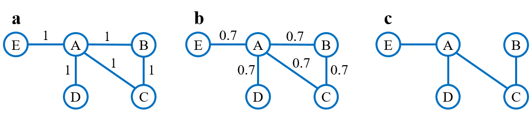
Since now edges are attached with probabilities, should eventually conform well with the scaled structural properties of in expectation. That is, we can define the expected degree of a node and the expected number of triangles and wedges the node belongs to, as the scaled local properties to specifically indicate the optimization goal. We also note that the expected number of wedges is often not as important as the (more prominent) expected number of triangles. Therefore, whether to preserve both the expected number of triangles and wedges associated with nodes depends on the application context.
II-B Sparsification via scaled local properties
To expand on [8, 9] and to take more than local degrees into account, we further consider -size subgraphs and propose a normalized definition of network sparsification. The expected degree of a node and the expected number of triangles and wedges the node belongs to have been defined in the context of uncertain graphs [11] and can also be applied here.
For a given and a randomly selected node , all possible neighbors of form the set with being the degree of in . Given , the corresponding set containing edge contributions is . Similarly, all possible triangles that belongs to form the set . The maximum possible number of triangles that can have in hence is and we also have .
By assuming the independence of edge probabilities [10], the expected degree of as well as the expected number of triangles and wedges that belongs to (respectively), are derived using the linearity of expectation as [11]:
| (1) |
| (2) |
| (3) |
where and iterate over the members of the sets and , respectively. An example for the calculation of Eqs. (1) and (2) is given in Figure 1b. For Eq. (3), if we let be a discrete random variable with , then it represents all possible degrees of during the edge sampling process. To obtain , we calculate by using dynamic programming based on [13].
In a sparse subgraph , each node should be as close as possible to its expected basic local properties. For this, we define the normalized distance from the current degree () of and the current number of triangles () and wedges () that belongs to in , to their expectations:
| (4) |
where is a normalization factor to distinguish the positions of different nodes. It emphasizes that the sparsification by edge sampling is built on top of the original network. Note that previous studies [8, 9, 10, 11] ignore this factor. We demonstrate its importance in Section IV-C. The total distance for a subgraph is therefore defined as:
Definition 1.
Given an undirected network and scaled local properties (on the expected degree of each node and the expected number of triangles and wedges each node belongs to) to be preserved, the distance of any subgraph to its overall expectation is:
| (5) |
The network sparsification problem via edge sampling is therefore defined as:
Definition 2.
(Sparsification via scaled local properties). Given an undirected network , find a subgraph such that:
| (6) |
By default, this is meant as the for all three properties together. In our experiments, we will also look at subsets thereof (degrees and triangles), though. According to Ref. [10], for this problem is a special case of the closest vector problem, which is -hard [14]. As our problem is a generalization, it is -hard, too. We hence aim at providing heuristic solutions that are fast and accurate enough for practical purposes.
III The game-theoretic sparsification with tolerance (GST)
Parchas et al. 2015 proposed a game-theoretic framework for uncertain graph sampling. It consists of an exact potential game with convergence to a Nash equilibrium based on best-response dynamics [15]. We adapt this framework to sparsification and include a tolerance factor that allows to terminate when the progress is below a user-specified threshold.
The basic idea is that each edge in a given is modeled as a player involved in an exact potential game. In this game, the gain change in the individual cost function is reflected in a global potential function. Specifically, each edge decides whether to be preserved (binary states: for preservation) in the final sparse graph . Suppose that the decision of changes the current into ; the current state of is updated only if this leads to a positive gain change (), which is defined as [11]:
| (7) |
where the sum of is the gain (or the distance to the overall expectation) of by retaining its current state, while the sum of is the gain of by changing its state. The result is the overall gain change resulting from the global potential function where each node is involved. Recall that we consider basic local properties: degrees and -node subgraphs (wedges and triangles). Only a limited number of nodes are therefore affected by a change in in Eq. (7). These nodes include , , and common neighbors of and in , forming a set we denote as . Therefore, as proved in [11], Eq. (7) is equivalent to:
| (8) |
which represents the change of the individual cost function. The equivalence of Eqs. (7) and (8) ensures that this game is an exact potential game. The best-response dynamics – that each edge repeatedly changes its state based on the decisions of all others – on the exact potential game guarantees the convergence to a Nash equilibrium [15]. That is, if the corresponding algorithm models this process, it will terminate.
Algorithm 1 presents the pseudocode of GST, which models such an exact potential game. We emphasize again that although we consider by default the preservation of the expected number of wedges () in GST, empirical studies still need to compare two cases: with and without . The inputs include an undirected network and two important values, the tolerance for early termination and the scaling factor for sparsification. Stage I (lines 1-5) computes the expected local properties based on and . The computation of Eqs. (1) and (2) are parallelized since they need only local information. Stage II initializes the current subgraph with the entire set in line 6. The in line 8 are therefore exactly the same as for . represents the set of all affected nodes and is initialized with the entire set . We include another array for recording during iterations. Starting from line 10, the algorithm proceeds in rounds. In each round, given an edge incident to a node in , it first finds all affected nodes in by the decision of . That is, includes , , and common neighbors of and in . Then, it computes induced by assuming that changes its current state. If and the removal of leads to a positive , then changes from to . If and the preservation of gives a positive , then switches from to . The iteration stops based on the progress in the gain in relation to the threshold .
for do in parallel 2
for do in parallel 5
repeat 6
for each incident (in ) to a node in do 7
until and 11
Regarding (sequential) time complexity, we note for Stage I that computing Eq. (1) takes time. When computing triangles, we use a merge-based intersection operation between and each of its neighbors, since each node already has a sorted neighbor set. Computing Eq. (2) therefore takes time in total, where is the maximum (possible) degree in . According to [16], an even tighter bound is , with being the arboricity of . Computing Eq. (3) via dynamic programming also takes time. Hence, the total time complexity of Stage I is .
Stage II depends mostly on the time spent on the repeat-loop. Finding involves a linear-time intersection operation with time each for two already sorted neighbor sets. For similar reasons as in Stage I, the for-loop takes time (per iteration of the repeat-loop). Stage II therefore needs in total, where is the number of iterations of the repeat-loop. Thus, in total, the time complexity of Algorithm 1 is . We show in Section IV-B how the tolerance threshold affects the convergence positively. Moreover, we present in Section IV-D the empirical running times of both stages.
IV Applications to climate data
We assess the performance of GST by answering the following three questions in Secs. IV-B, IV-C, and IV-D, respectively:
- Q1:
How well does GST generate a sparse preserving scaled local properties?
- Q2:
How well does GST generate a sparse preserving non-local / complex properties?
- Q3:
How is the running time of GST?
| Network | Nodes () | edges () | Edge confidence () | |
|---|---|---|---|---|
| Glo_ERA5SP | 7,320 | 593,736 | 81.11 | 1 |
| Glo_ERA5ST | 7,320 | 882,102 | 120.51 | 1 |
| Glo_TRMM | 36,000 | 2,139,214 | 59.42 | [0.99, 1] |
| ASM_TRMM | 20,000 | 1,771,609 | 88.58 | [0.99, 1] |
IV-A Experimental settings
(1) Climate data sets. Our particular focus on climate data is mainly driven by studies of complex climate phenomena using complex networks during the last two decades. The reconstructed functional climate networks can be large especially when a high spatial resolution is considered. Four functional networks are summarized in Table II. If , then the corresponding networks are completely deterministic:
- •
Glo_ERA5SP: we use the time series of daily surface level pressure (SP) within the June-July-August season from 1998 to 2019 from ERA5 reanalysis data [17], with the global spatial resolution of 1∘ 1∘. The functional network reconstruction process is adapted from [18] by viewing grid points as nodes and using Spearman correlation as the similarity between time series.
- •
Glo_ERA5ST: it is the same as Glo_ERA5SP, but using daily surface level temperature (ST) [17].
- •
Glo_TRMM: we consider the observational data of global precipitation from Tropical Rainfall Measuring Mission 3B42v6 product (TRMM) [19]. Time series represent the daily rainfall sums within the June-July-August season from 1998 to 2019 with a spatial resolution of . As precipitation data are spiking series, we adopt event synchronization (ES) as a nonlinear similarity measure [20]. By treating grid points as nodes, the reconstruction process is the same as in [1].
- •
ASM_TRMM: it is the same as Glo_TRMM, but focuses on a relatively small region, i.e., the Asian summer monsoon (ASM) region, instead of the global scale.
(2) Baselines. We compare GST with four baselines. Zeng et al. 2021, Zeng et al. 2022 studied preserving the expected degree of each node and adapted two approximate methods similar to those in uncertain graph sampling [11]. Parchas et al. 2015 concluded that among all approximate methods they proposed, the game-theoretic framework generates better representative instances. We directly adapt this framework for network sparsification. In particular, GST2 preserves only the scaled degrees and corresponds to [8, 9]. Therefore, the first comparison is between GST2 and our extensions GST2,3/GST2,3,w, where and denote 3-node subgraphs (triangles and wedges, respectively) associated with each node (see Section IV-B). Other three well-known sampling methods are local degree (LD) [2], local jaccard similarity (LJS) [21], and random edge (RE) [4] (see Section IV-C). We choose them due to their effectiveness in preserving the overall connectivity (by LD), community structure (by LJS), and spectral property (by RE), at least in non-functional networks. They have been systematically compared in [2] and implemented in NetworKit [22], a tool suite for scalable network analysis.
(3) Evaluation metrics. For Q1, we analyze the extent to which the expected degree and the expected number of 3-node subgraphs associated with each node are preserved, even when bearing some loss with the inclusion of a tolerance threshold in GST. The four measures below are used (see Section IV-B):
- •
Node-wise distance distribution: . It represents the summarized overall distance of the local properties (degrees, triangles, and wedges) for each node in the generated to the expectation. Hence, is a sequence of length . The minimization of the sum of over all nodes corresponds to the objective of Eq. (6).
- •
Mean distance: .
- •
Convergence of mean distance: . This measure is designed for convergence analysis, since it is based on the current (at line 20 of Algorithm 1) instead of .
- •
Cumulative time: total time spent until the current iteration (lines 10-25 in Algorithm 1), also for empirical convergence analysis.
For Q2, the following property queries are considered: macroscopic: the global clustering coefficient and largest connected component; mesoscopic: community structure and betweenness centrality; microscopic: degree and local clustering coefficient. Both mesoscopic and microscopic queries have been applied in functional climate network analysis [1, 18]. In particular, computing the exact betweenness values is in practice very expensive for the unsparsified network. Therefore, we use ApproxBetweenness from NetworKit [22] with a guarantee that the error is no larger than 0.01, with a probability of at least 0.9. Measures used to estimate the similarity between the properties calculated from and are (see Section IV-C):
- •
Average Deviation [2]: we analyze the deviation of the macroscopic properties in from those in , because these properties are single-valued representations.
- •
Average Adjusted rand index (ARI) [23]: this one is particularly used for giving the similarity between two clusterings obtained based on the final sparse network and the original network , respectively.
- •
Average Spearman rank correlation coefficient [2]: microscopic properties are node-wise representations, therefore similarities are estimated using correlation with a significance level of .
The estimation process is as follows. Taking the comparison between GST2,3() and LD as an example, we first generate 100 sparse networks for a given , based on GST2,3(). Then, another 100 sparse networks, say LD, are created by using LD with the preservation ratio of edges calculated based on the edge ratio between and . Assuming the query on community structure, we apply the parallel Louvain method [24] from NetworKit [22] to , , and LD, respectively. We then compute the ARI between the highest-quality (out of 100 repeated runs) community structures obtained from and each ; the same process is applied to and each LD. One can notice that it is hard to ensure that one edge sampling method outperforms the rest for all of these property queries. Therefore, we need additional measures summarizing all queries, instead of checking them one by one (see Section IV-C):
- •
Ranking distribution: for each given scaling factor , each query task gives a ranking between GST, LD, LJS and RE, from 1 to 4. We summarize all rankings of each method for different and property queries.
- •
Mean ranking: the mean of all rankings of each method.
For Q3, to give a fair comparison between GST, LD, LJS, and RE (see Section IV-D), we choose a single-threaded environment without parallelization. The comparison shows the average running time over 100 runs.
IV-B Basic property preservation
We show the distribution of using boxplots and in Figures 2, 3, 4 and 5. The preservation scenarios which include 3-node subgraphs (triangles and wedges) are highlighted with hatches (see GST2,3 and GST2,3,w). Regarding Q1, we conclude that preserving both the expected degrees and the expected number of 3-node subgraphs generates sparse structures closer to the expectation than only considering degrees. This fact holds even when the tolerance is set to . From here on we focus only on GST2,3 and GST2,3,w.


As for the convergence and cumulative time of GST, due to limited space, we show the result for Glo_ERA5SP as an example in Figure 6; results for the other three networks are similar to this one. When the tolerance is empirically given, the convergence of strictly follows the convergence trajectories of , as it should be. The final running times of GST2,3() and GST2,3,w() (blue circles) are at least 4 times faster than that of GST2,3() and GST2,3,w() (blue triangles). More importantly, the qualities of the final sparse structure by (the last black circles) are still quite close to those of (the last black triangles).
IV-C Complex property preservation
As for property queries, how to compare the similarity estimates obtained for different queries is not obvious, as mentioned in Section IV-A. We therefore give such a similarity result only for Glo_ERA5SP as an example in Figure 7, and focus on overall rankings in Figure 8. In Figure 7, GST2,3() and GST2,3,w() are quite good at preserving degrees (see Figure 7c), which can be expected due to the explicit preservation of scaled degrees. Although Hamann et al. 2016 concluded that LD is best for preserving the overall connectivity of a network, we here see from Figures 7a and 7b that LJS is even better. This should be due to different network structures in different domains. They use mostly social networks, while we focus on functional climate networks. Another noteworthy point is that for a given scaling factor , only similarity estimates of community structure show a slightly larger variance. This suggests the stability of all these sampling methods applicable for practical scenarios. Still, comparing different queries in Figure 7 is not conclusive due to the diverse performance of the different methods. We thus summarize Figure 7 in Figure 8a by using their rankings.
In Figure 8a, GST2,3() ranks first in the comparisons of both median (red dash lines) and mean (blue dots) rankings. From Figure 8, one can conclude that, for a given , a good performance of GST2,3() does not guarantee that GST2,3,w() also has a similarly good performance. For example, GST2,3() works better for Glo_ERA5SP, Glo_ERA5ST, and ASM_TRMM, while GST2,3,w() is better for Glo_TRMM and ASM_TRMM. We conjecture that this is due to the diversity of different network structures, as we expected in Secs. II-A and III. Nonetheless, either one of our two methods is always the best. Thus, preserving both scaled degrees and 3-node subgraphs yields a sparser graph that better preserves complex properties overall. This answers Q2.
We also compare GST2,3() with UNGST2,3() to verify the necessity of including a normalization factor in Eq. (4), where UNGST2,3() is an unnormalized version of GST by removing from Eqs. (4) and (8) this normalization factor. The same estimation process based on the above six property queries is adopted and the summarized rankings are shown in Figure 9. UNGST2,3() proceeds until the final convergence instead of early convergence, since . GST2,3() still generates sparse networks with a higher similarity to the original Glo_ERA5SP properties.
IV-D Running times
To answer Q3, we compare the running times of GST, LD, LJS and RE in Figure 10. Taking Glo_ERA5SP as an example, GST2,3() is chosen as the sampling method based on Figure 8a. For each given scaling factor , GST2,3() generates 100 sparse subgraphs . We calculate the average and deviation of running time for both stages of Algorithm 1. The edge ratio between and is used for the initialization of LD, LJS, and RE, further to obtain the corresponding running time.
According to [2], the running times of LD and LJS are slightly slower than RE, which only takes linear time in the number of edges. The running time of GST mainly depends on the number of iterations in Stage II, even with a tolerance factor included for early termination. In Figure 10, GST is therefore roughly 19, 12, and 90 times slower than LD, LJS, and RE, respectively. Nonetheless, GST is still applicable to large-scale networks.
V Conclusion
In summary, we proposed a different perspective (by preserving scaled local node characteristics) from the general filtering-based sampling methods for network sparsification. Our empirical studies on functional climate networks verify that the proposed method generates sparse subgraphs that preserve the overall similarity to the original network in a considerably better way.
As future work, we will further study the robustness of this method in other network application scenarios as well as for synthetic data. Which preservation of -node subgraphs ( or ) one should choose for best results on a wide range of unknown data sets remains as another issue not fully settled yet.
Acknowledgements
We would like to thank Panos Parchas for data sharing. Z.S. was funded by the China Scholarship Council (CSC) scholarship. J.K. was supported by the Federal Ministry of Education and Research (BMBF) grant No. 01LP1902J (climXtreme). H.M. was partially supported by German Research Foundation (DFG) grant ME-3619/4-1 (ALMACOM).
References
- Su et al. [2022] Z. Su, H. Meyerhenke, and J. Kurths, “The climatic interdependence of extreme-rainfall events around the globe,” Chaos: An Interdisciplinary Journal of Nonlinear Science, vol. 32, no. 4, p. 043126, 2022.
- Hamann et al. [2016] M. Hamann, G. Lindner, H. Meyerhenke, C. L. Staudt, and D. Wagner, “Structure-preserving sparsification methods for social networks,” Social Network Analysis and Mining, vol. 6, no. 1, p. 22, 2016.
- Batson et al. [2013] J. Batson, D. A. Spielman, N. Srivastava, and S.-H. Teng, “Spectral sparsification of graphs: Theory and algorithms,” Communications of the ACM, vol. 56, no. 8, pp. 87–94, 2013.
- Sadhanala et al. [2016] V. Sadhanala, Y.-X. Wang, and R. Tibshirani, “Graph Sparsification Approaches for Laplacian Smoothing,” in Proceedings of the 19th International Conference on Artificial Intelligence and Statistics. PMLR, 2016, pp. 1250–1259.
- Mahadevan et al. [2006] P. Mahadevan, D. Krioukov, K. Fall, and A. Vahdat, “Systematic topology analysis and generation using degree correlations,” ACM SIGCOMM Computer Communication Review, vol. 36, no. 4, pp. 135–146, 2006.
- Orsini et al. [2015] C. Orsini, M. M. Dankulov, P. Colomer-de-Simón, A. Jamakovic, P. Mahadevan, A. Vahdat, K. E. Bassler, Z. Toroczkai, M. Boguñá, G. Caldarelli, S. Fortunato, and D. Krioukov, “Quantifying randomness in real networks,” Nature Communications, vol. 6, no. 1, p. 8627, 2015.
- Benzi and Klymko [2015] M. Benzi and C. Klymko, “On the Limiting Behavior of Parameter-Dependent Network Centrality Measures,” SIAM Journal on Matrix Analysis and Applications, vol. 36, no. 2, pp. 686–706, 2015.
- Zeng et al. [2021] Y. Zeng, C. Song, and T. Ge, “Selective Edge Shedding in Large Graphs Under Resource Constraints,” in 2021 IEEE 37th International Conference on Data Engineering (ICDE), 2021, pp. 2057–2062.
- Zeng et al. [2022] Y. Zeng, C. Song, T. Ge, and Y. Zhang, “Reduction of large-scale graphs: Effective edge shedding at a controllable ratio under resource constraints,” Knowledge-Based Systems, vol. 240, p. 108126, 2022.
- Parchas et al. [2014] P. Parchas, F. Gullo, D. Papadias, and F. Bonchi, “The pursuit of a good possible world: Extracting representative instances of uncertain graphs,” in Proceedings of the 2014 ACM SIGMOD International Conference on Management of Data, ser. SIGMOD ’14. New York, NY, USA: Association for Computing Machinery, 2014, pp. 967–978.
- Parchas et al. [2015] ——, “Uncertain Graph Processing through Representative Instances,” ACM Transactions on Database Systems, vol. 40, no. 3, pp. 20:1–20:39, 2015.
- Song et al. [2016] S. Song, Z. Zou, and K. Liu, “Triangle-Based Representative Possible Worlds of Uncertain Graphs,” in Database Systems for Advanced Applications, ser. Lecture Notes in Computer Science, S. B. Navathe, W. Wu, S. Shekhar, X. Du, S. X. Wang, and H. Xiong, Eds. Cham: Springer International Publishing, 2016, pp. 283–298.
- Bonchi et al. [2014] F. Bonchi, F. Gullo, A. Kaltenbrunner, and Y. Volkovich, “Core decomposition of uncertain graphs,” in Proceedings of the 20th ACM SIGKDD International Conference on Knowledge Discovery and Data Mining, ser. KDD ’14. New York, NY, USA: Association for Computing Machinery, 2014, pp. 1316–1325.
- Micciancio [2001] D. Micciancio, “The hardness of the closest vector problem with preprocessing,” IEEE Transactions on Information Theory, vol. 47, no. 3, pp. 1212–1215, 2001.
- Monderer and Shapley [1996] D. Monderer and L. S. Shapley, “Potential Games,” Games and Economic Behavior, vol. 14, no. 1, pp. 124–143, 1996.
- Ortmann and Brandes [2013] M. Ortmann and U. Brandes, “Triangle Listing Algorithms: Back from the Diversion,” in 2014 Proceedings of the Meeting on Algorithm Engineering and Experiments (ALENEX), ser. Proceedings. Society for Industrial and Applied Mathematics, 2013, pp. 1–8.
- Hersbach et al. [2020] H. Hersbach, B. Bell, P. Berrisford, S. Hirahara, A. Horányi, J. Muñoz-Sabater, J. Nicolas, C. Peubey, R. Radu, D. Schepers, A. Simmons, C. Soci, S. Abdalla, X. Abellan, G. Balsamo, P. Bechtold, G. Biavati, J. Bidlot, M. Bonavita, G. De Chiara, P. Dahlgren, D. Dee, M. Diamantakis, R. Dragani, J. Flemming, R. Forbes, M. Fuentes, A. Geer, L. Haimberger, S. Healy, R. J. Hogan, E. Hólm, M. Janisková, S. Keeley, P. Laloyaux, P. Lopez, C. Lupu, G. Radnoti, P. de Rosnay, I. Rozum, F. Vamborg, S. Villaume, and J.-N. Thépaut, “The ERA5 global reanalysis,” Quarterly Journal of the Royal Meteorological Society, vol. 146, no. 730, pp. 1999–2049, 2020.
- Gupta et al. [2021] S. Gupta, N. Boers, F. Pappenberger, and J. Kurths, “Complex network approach for detecting tropical cyclones,” Climate Dynamics, vol. 57, no. 11, pp. 3355–3364, 2021.
- Huffman et al. [2007] G. J. Huffman, D. T. Bolvin, E. J. Nelkin, D. B. Wolff, R. F. Adler, G. Gu, Y. Hong, K. P. Bowman, and E. F. Stocker, “The TRMM Multisatellite Precipitation Analysis (TMPA): Quasi-Global, Multiyear, Combined-Sensor Precipitation Estimates at Fine Scales,” Journal of Hydrometeorology, vol. 8, no. 1, pp. 38–55, 2007.
- Quian Quiroga et al. [2002] R. Quian Quiroga, T. Kreuz, and P. Grassberger, “Event synchronization: A simple and fast method to measure synchronicity and time delay patterns,” Physical Review E, vol. 66, no. 4, p. 041904, 2002.
- Satuluri et al. [2011] V. Satuluri, S. Parthasarathy, and Y. Ruan, “Local graph sparsification for scalable clustering,” in Proceedings of the 2011 ACM SIGMOD International Conference on Management of Data, ser. SIGMOD ’11. New York, NY, USA: Association for Computing Machinery, 2011, pp. 721–732.
- Staudt et al. [2016] C. L. Staudt, A. Sazonovs, and H. Meyerhenke, “NetworKit: A tool suite for large-scale complex network analysis,” Network Science, vol. 4, no. 4, pp. 508–530, 2016.
- Vinh et al. [2010] N. X. Vinh, J. Epps, and J. Bailey, “Information Theoretic Measures for Clusterings Comparison: Variants, Properties, Normalization and Correction for Chance,” Journal of Machine Learning Research, vol. 11, no. 95, pp. 2837–2854, 2010.
- Staudt and Meyerhenke [2016] C. L. Staudt and H. Meyerhenke, “Engineering Parallel Algorithms for Community Detection in Massive Networks,” IEEE Transactions on Parallel and Distributed Systems, vol. 27, no. 1, pp. 171–184, 2016.