Spin Transport in Magnetically Ordered Systems: Ferromagnets, Antiferromagnets and Frustrated Systems
Abstract
In this review, we outline the important results on the resistivity encountered by an electron in magnetically ordered materials. The mechanism of the collision between the electron and the lattice spins is shown. Experiments on the spin resistivity in various magnetic materials as well as theoretical background are recalled. We focus on our works since 15 years using principally Monte Carlo simulations. In these works, we have studied the spin resistivity in various kinds of magnetic systems ranging from ferromagnets and antiferromagnets to frustrated spin systems. It is found that the spin resistivity shows a broad peak at the transition temperature in systems with a second-order phase transition, while it undergoes a discontinuous jump at the transition temperature of a first-order transition. New results on the hexagonal-close-packed (HCP) antiferromagnet are also shown in extended details for the Ising case in both the frustrated and non-frustrated parameter regions.
Keywords:
spin resistivity; ferromagnets; antiferromagnets; frustrated spin systems; Monte Carlo simulationI Introduction
The resistivity encountered by the displacement of an electron driven by an applied electric field in a material is due to its collisions with the material constituents such as atoms. In general these collisions are caused not by direct contacts but by various potentials, magnetic and electric fields from different sources. As a matter of fact, the motion of the electron is slowed down except in the superconducting regime. One can mention many simple examples such as the motion of an electron in a magnet, or in a lattice with vibrating atoms (phonons) under an applied electric field.
The investigation of the resistivity is one of the most important tasks in condensed matter physics. Apart from the desire to understand the mechanisms lying behind the resistivity, the numerous applications using the transport properties of electrons in electronic devices have motivated an increasing number of studies, experimentally, theoretically and numerically. The study of the resistivity has started after the discovery of the electron more than a century ago by the simple free-electron Drude theory taking into account the relaxation time between two successive collisions due to atoms. The following relation has been established
| (1) |
where is the conductivity, the electron charge, the electron relaxation time, the electron mass, and the number of electrons crossing a unit srface per unit of time.
Over the years, there has been a large number of more realistic theories of resistivity which take into account different interactions. Nevertheless, this relation is still valid if the electron mass is replaced by its effective mass which includes effects of the interactions of the electron with its environment. The relaxation time should also be modified, it is no more a constant but it depends on the collision mechanism. In a crystal it is known that the effective mass of the electron can be ”heavier” or ”lighter” than its mass at rest because it contains the effects of various interactions. This strongly modifies the mobility of the electron in crystals. As for , it has a strong effect on the temperature dependence of the resistivity. It has been established that depends on a power of the electron energy. This power depends on the collision process such as collisions with charged impurities, neutral impurities, magnetic impurities, phonons, magnons, etc. Thus, in a crystal the total resistivity is a sum of the contributions coming from various collision processes. At low temperature (), it is given by
| (2) |
where , and are constants. The first term is -independent, the second term, proportional to , stems from the scattering of the conducting electron at low by lattice spin-waves. Note that the resistivity caused by a Fermi liquid is also proportional to with another coefficient. The term which is observed in metals comes from the diffusion of conduction electrons by atomic vibrations. However, the resistivity in metals show a linear- dependence at high . The last term expresses the contribution from the quantum Kondo effect, namely the scattering of conduction electrons by magnetic impurities at extremely low .
In this review, we focus our attention on the resistivity due to the spin of the conduction electron in magnetically ordered materials. For short let us call it the ”spin resistivity” hereafter. This spin resistivity has been widely studied both experimentally and theoretically for more than five decades. The rapid development of the field is due mainly to many applications in spintronics.
We are interested in magnetic materials which show a phase transition from a magnetically ordered phase, such as ferromagnets and antiferromagnets, to the paramagnetic state. Let us mention in the following some experiments which have been performed in magnetic materials including metals, semiconductors and superconductors. These experiments carried out on various materials show different shapes of the spin resistivity around the phase-transition temperature: SrRuO3 thin films Xia, Ru-doped La0.4Ca0.6MnO3 Lu2009, antiferromagnetic -(Mn1-xFex)3.25Ge Du2007, semiconducting Pr0.7Ca0.3MnO3 thin films Zhang, superconducting BaFe2As2 single crystals Wang-Chen, LaFeAsO McGuire2008 and La1-xSrxMnO3 Santos2009. We see in these works that depending on the nature of the compound, can have a pronounced peak Matsukura or a change of its slope, or a curvature change at the transition temperature . Note that in the last case, one has a maximum of the differential resistivity Stishov; Shwerer.
Theoretically, the magnetic contribution in Eq. (2) has been obtained by Kasuya Kasuya taking into account the scattering of the electron spin by the spin waves at low . However, at higher , specially in the region of the phase transition of the magnetic lattice, there has been no such clear mechanisms explaining different experimental behaviors of the spin resistivity. de Gennes and Friedel DeGennes have conjectured that the spin resistivity has the origin in the spin-spin correlation so it should behave as the magnetic susceptibility. As a consequence, it should diverge at . However, Fisher and Langer Fisher, and Kataoka Kataoka have made the observation that the range of spin-spin correlation should not be infinite at due to collisions. This changes the shape of with respect to the magnetic susceptibility near the phase transition. Let us mention that the resistivity due to magnetic impurities has been calculated by Zarand et al. Zarand as a function of the Anderson’s localization length. This parameter expresses in fact a kind the correlation sphere induced around each impurity. Their result shows that the resistivity peak depends on this parameter, thus in agreement with the spin-spin correlation idea.
Note that the spin resistivity depends on the spin orientation of the environment: the electron encounters less resistance in a ferromagnet with spins parallel to its spin than in a ferromagnet with spins antiparallel to its spin. Imagine a film composed of three ferromagnetic layers where the middle one is a soft ferromagnet. In the layer-coupling configuration , the movement of an up spin perpendicular to the film encounters a resistance . One applies now an external magnetic field in the negative direction, small enough to reverse the spins in the (middle) soft layer: one has the three-layer configuration . The up spin is found to encounter much difficulty to cross the three layers: the resistance is which is much larger than . This is the phenomenon Giant-Magneto-Resistance (GMR) discovered in Refs. Fert1; Fert2; Grunberg which has many applications in spintronics.
The absence of Monte Carlo (MC) simulation in the literature on the spin resistivity has motivated our works since 2007: we have studied the spin current in a number of systems including ferromagnets Akabli; Akabli2; Akabli3 and antiferromagnets Akabli4; Magnin; Magnin3; Magnin2012 by MC simulations. The behavior of as a function of has been shown to be in general agreement with experiments and theories mentioned above. In addition to ferromagnets and antiferromagnets, we have also studied the spin resistivity in frustrated spin systems Magnin2; Hoang2011. These systems discovered in the early 80’s have been intensively studied. Many unusual properties have been found. The reader is referred to Ref. DiepFSS for reviews on various frustrated spin systems. In this paper, we will summarize the most important aspects and results of works on the spin resistivity in ferromagnets, antiferromagnets and in some frustrated magnets.
In section II, we present our generic model and the MC method which we employ to study the spin resistivity. Section III is devoted to the presentation of our main MC results since 2007. Comparison with some experiments is made in this section. In section IV, we show new results in the case of a hexagonal-close-packed (HCP) crystal where we tune a frustration parameter allowing to study both the non-frustrated case and the frustrated case in the phase space. Conclusing remarks are given in section V.
II Model and Method
II.1 Model
We have investigated the spin resistivity in magnetically ordered materials by using a newly-deviced efficient MC simulation method Magnin; Magnin3. The success of the method was demonstrated when we studied the semiconducting MnTe where the agreement with experiment is excellent Magnin2012. This case will be reviewed below. In ferromagnets, we found that the spin resistivity has a high peak at the lattice order-disorder transition tremperature . As said earlier, this anomaly comes from the spin-spin correlation DeGennes; Fisher; Kataoka but remains finite at . In antiferromagnets, one observes only a broad maximum Haas. In addition to ferromagnets and antiferromagnets, we have investigated the spin resistivity in the following two frustrated systems: the face-centered cubic (FCC) lattice with Ising spins Magnin2 and the simple cubic (SC) lattice Hoang2011. We found that that the first-order phase transition in these frustrated systems causes a discontinuity of the spin resistivity at .
Let us recall here the model and method which have been used in our early works shown in Refs. Magnin; Magnin2: simulations have been carried out to calculate the current of itinerant spins moving in the system under the action of an electric field applied in the direction. The itinerant spin carried by a conduction electron interacts with its surrounding lattice spins inside the sphere of radius centered at its position at the time on its trajectory across the crystal. The Hamiltonian is supposed to be
| (3) |
where the sum is carried over all lattice spins in the sphere centered at the itinerant Ising spin . denotes the distance-dependent interaction between and . To be general, we also consider the following interaction between an electron spin with neighboring conduction spins within a sphere of radius
| (4) |
For simplicity, we suppose the distance-dependent interactions are
| (5) | |||||
| (6) |
where , , and are constants to be chosen so that the energy of a conduction electron spin is much smaller than that of a lattice spin. This choice is made from a physical consideration: in choosing so, we avoid the influence of itinerant spins on the ordering of the lattice spins. Note that this choice is justified in the almost-free electron model where , and in semiconductors where they are larger but still weak with respect to the exchange intergrals of the lattice spins and . A discussion in details on the choice of these parameters has been given for example in Ref. Magnin.
Let us assume in the folklowing a concentration of one itinerant electron per two lattice cells. This concentration is thus of the order of electron concentration in normal metals which is . With this concentration, it is obvious that the averaged distance between two conduction electrons is much larger than the cutoff distance which is of the order of the lattice constant. However, due to the attractive nature of the electron-electron interaction, Eq. (6), it is neccessary to introduce a chemical potential term to insure that itinerant spins are uniformmly dispersed in the crystal and they do not form clusters. This chemical potential is written as
| (7) |
where is a positive constant, denotes the concentration of conduction spins in the sphere of cutoff radius centered at the position of the conduction spin under consideration, and the averaged electron concentration.
is defined in Eq. (5) which represents the magnitude of the interaction between a conduction electron and a localized lattice spin [Eq. (3)]. is the magnitude of the interaction between two conduction electrons [see Eq. (4) and (6)]. is the magnitude of the chemical potential [Eq. (7)]. When we simulate a real material, if we have experimental data on the resistivity and the exchange interactions, such as in the case MnTe presented in section III.3, we can estimate the values of these coefficients.
II.2 Simulation Method
Let us study a film of size where is the film thickness which is much smaller than the sizes and in the and , respectively. Usually, we use and . Itinerant spins move under the action of an electric field acting on the electron charge, applied in the direction . The electric field energy is
| (8) |
where is the electron charge, the applied electrical field and the displacement vector of the electron.
The interaction between the lattice spins is given by the Hamiltonian
| (9) |
where is the exchange interaction between nearest neighbors (NN) and . For ferromagnets , and for antiferromagnets .
We use the standard Monte Carlo (MC) method to thermalize the lattice alone at . Next, we introduce the electrons into the lattice. We suppost that each electron spin interacts with the surrounding lattice spins inside a sphere centered at its position, of radius . The electron spin also interacts with other electron spins within a sphere of radius . Electrons move under the applied electric field.
In order to obtain the spin current we have to thermalize the state of the spins of conduction electrons in the lattice. This is done by the following steps:
i) we take a conduction spin and calculate its actual energy using the different interactions mentioned above,
ii) we make a trial move for the electron in a random direction between 0 and where is the lattice constant. If the move takes the itinerant electron outside the sample, then we put it inside on the other sample end by virtue of the periodic boundary condition,
iii) we then calculate the new energy . If , then the trial position is accepted. Otherwise, it is accepted with the probability .
iv) we take another conduction electron and repeat the three steps above. We continue with other electrons until all electrons are considered: this accomplishes one MC step/spin. A large number of MC steps/spin is neccessary to arrive at a steady current state. We next average physical quantities of interest at the temperature under consideration.
iv) we take another and repeat the above four steps. We should cover the temperature region of interest.
This paper is a review of our publications over the past 15 years. In each publication, we used various sample sizes to detect finite size effects. We increased the sample size until the results do not depend anymore on the size. The results are considered as valid thermodynamically. The finite size effect and the finite size scaling are what the simulators do before reaching conclusions. This problem is particularly important when one wants to study the criticality or the order of a phase transion. In the review, we do not repeat these details which depend on the studied system. Rather, we emphasize on the results. The reader interested on the details of the simulation methods is referred to each original publication.
We calculate the spin resistivity as :
| (10) |
where is the number of mobile electrons passing thru a unit surface perpendicular to the direction of the applied electric field , per MC time unit. An application with a real material using real units is presented in subsect. III.3.
For a good thermal average, we have to perform very long MC runs and we proceed as follows: for each configuration of the lattice spins we average the spin resistivity over MC steps, then we thermalize again the lattice with MC steps to get rid of the correlation between lattice spin configurations, before averaging again the resistivity for MC steps. We repeat this cycle for a large number of times . The total MC steps of resistivity averaging is about steps per spin in our runs. We found by comparison that this ”multi-step” averaging method strongly suppresses statistical fluctuations seen in our earlier work Akabli2.
It is obvious that the larger and yields the better statistics. We know that depending on , the relaxation time of the lattice spins varies. We have to compare with the relaxation time of conduction electron spins in order to choose a right value of in order to calculate the average of the resistivity with one lattice spin configuration at . We know the two limiting cases. The first case is when . In this case, we have to take , namely the lattice spin configuration should change with each move of itinerant spins. The second case is when . In this case itinerant spins can be scattered many times along its trajectory across the same lattice configuration and for many times across the lattice.
In order to choose a right value of , we consider the following temperature dependence of in non frustrated spin systems. The relaxation time is expressed in this case as Hohenberg; Peczak; Prudnikov
| (11) |
where is a constant, the correlation critical exponent, and the dynamic exponent which depends on the spin model and space dimension. For 3D Ising model, and . From this expression, we see that as tends to , diverges. In the critical region around the system encounters thus the so-called ”critical slowing down”: the spin relaxation is extremely long due to the divergence of the spin-spin correlation. When we take into account the temperature dependence of , the shape of the resistivity is strongly modified near where is very long, in contrast to the paramagnetic phase where the relaxation time is very short due to rapid thermal fluctuations. We should emphasize that at low , does not depend on since in that temperature range where the ordering of the lattice spins is almost perfect: the spin landscape from one microscopic state to another does not change significantly, so the motion of the itinerant electron spin does not significantly vary (see Ref. Magnin3).
Finally, we note that we have also used the Boltzmann’s equation combined with MC data to study the spin resistivity Akabli3. However, the shape of the resistivity peak at the transition temperature does not agree well with experiments, unlike that obtained from direct MC simulations as shown below. This proves the efficiency of MC simulations for the calculation of the spin resistivity in magnetically ordered materials. The present review therefore aims at promoting this method.
III Review
III.1 Spin Resistivity in Ferromagnets and Antiferromagnets
Experiments mentioned above amongst numerous other data show that the spin resistivity in ferromagnets has a sharp peak at the transition temperature of the lattice. We know by the theory of phase transitions and critical phenomena that in the region around , the so-called ”critical slowing-down” phenomenon happens, resulting in extremely large . The peak in is due to this phenomenon via Eq. (11) where diverges at . Our MC simulations using the method described above in the case of a ferromagnet where the lattice spins are of the Ising type show a sharp peak at (see Fig. 1) in agreement with experimental data. We note that the spin resistivity for ferromagnets (as well as for antiferromagnets) increases with decreasing at low . This can be explained by several causes: the freezing or crystallization of conduction electrons takes place at low so that just a small number of conduction spins with decreasing is mobile, or it may be the classical counter effect of the quantum Kondo electron-impurity scattering if one considers the few excited lattice spins at low are independent impurities, see the last term of Eq. (2). Note that the shape of depends on the lattice type, interaction strengths encountered by the conduction electrons, electron concentration, relaxation time, spin model, applied magnetic-field amplitude etc. In Ref. Magnin, we have shown that a decrease in the interaction between conduction spins, , reduces the increase of as , an applied magnetic field reduces the height of the resistivity peak and the larger electron density reduces . Finally, we emphasize that depends on the material intrinsically via the critical exponents and , see Eq. (11).
If we wish to compare simulated spin resistivity to experimental measurements performed on a given material, we have to use in the simulation the available experimental physical parameters of that material. An example of quantitative comparison for semiconductor MnTe is shown in subsection III.3.

Note that the magnetic field applied on the system reduces the peak height as shown in our work Ref. Magnin, in agreement with experiments Lu2009.
Unlike ferromagnets, antiferromagnets have not been much studied. Haas Haas has shown that in contrat to ferromagnets where the resistivity has a sharp peak at the order-disorder transition of the lattice spins, in antiferromagnets there is no such a peak. Using MC simulations, we found that the peak does exist in an antiferromagnet but it is less sharp compared to that of a ferromagnet, as seen in Fig. 1. We think that the alternate change of sign of the spin-spin correlation with distance may have something to do with the absence of a sharp peak. We have tested this idea on the effect of the cut-off distance Magnin2: in an antiferromagnet, when we increase , we will include successively up-spin shells and down-spin shells in the sphere of radius . Consequently, the difference between the numbers of up and down spins in the sphere oscillates with varying , giving rise to the oscillatory behavior of observed at small , unlike in ferromagnets.
At this stage, we note that the presence of an itinerant spin will break the invariance between a ferromagnet and its antiferromagnet counterpart in the local Mattis transformation ().
III.2 Frustrated Model on a Simple Cubic Lattice
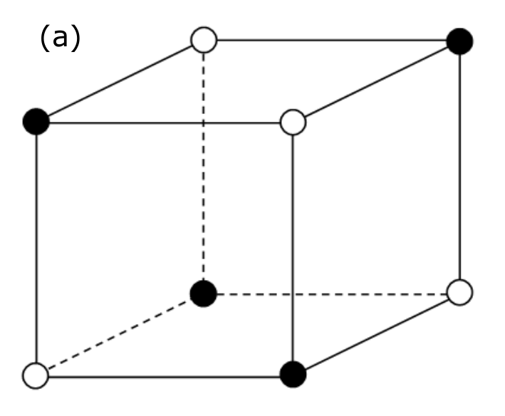
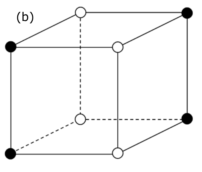
Let us consider the simple cubic lattice with NN and NNN interactions as shown in Fig. 2. The Hamiltonian is written as
| (12) |
where the first sum is made over the NN Ising spin pairs and with interaction , and the second sum is performed over the NNN pairs with interaction .
We focus our attention on the region of parameters which gives rise to a frustration. For that purpose, we assume that is an antiferromagnetic interaction, namely (), and is also antiferromagnetic. We put where is a positive parameter. The ground state (GS) of this system can be obtained by minimizing the energy, or by comparing the energies of different spin configurations. We can also numerically minimize the energy by using the steepest descent method Ngo2007. We obtain the GS antiferromagnetic configuration shown Fig. 3a for , and the GS spin configuration shown in Fig. 3b for . This latter configuration is 3-fold degenerate because we can choose the parallel NN spins either on , or or axis. In addition, with the permutation of black and white spins, we have the total degeneracy equal to 6.

We note in passing that in the case of the Heisenberg model in the frustrated region () the phase transition has been shown to be of first order Pinettes. The system is very unstable due to its large degeneracy. In the case of the Ising spin on the SC lattice treated here, we found that the first-order character of the phase transition is even stronger Hoang2011.
We use (AF interaction) for the coupling between NN lattice spins in the simulations. The energy is thus measured in the unit of and the temperature is in the unit of . All distances ( and ) are in the unit of the lattice constant .
Simulations have been carried out by using the temperature-dependent relaxation time of the lattice spins given by Eq. (11) where we have taken and at far from . Such a choice leads to at that temperature expected for fast thermal fluctuations in the paramagnetic phase far above .
Since we suppose that the interaction between conduction electron spins is attractive, a chemical potential is required to avoid the collapse of the system, namely to avoid that all conduction spins form a cluster [cf. Eq.(7)]. The chemical potential in thermodynamics makes the particle uniformly distributed in the space. Its strength is expressed by which has to be chosen in accordance with . Figure 4 displays the phase diagram in the space which shows the collapse region. This allows us to avoid this region and choose an appropriate value of for a given .
To see the effect of the nature of phase transition on the spin resistivity, in the following we focus on two typical cases: and which belong respectively to the regions of second- and first-order transition.
A. For :
The spin resistivity at temperatures below oscillates with varying . By analyzing the ratio of the number of up spins to the number of down spins in the sphere of radius , we found that it oscillates with varying : the maxima (minima) of correspond to the case of largest (smallest) numbers of parallel (antiparallel) spins in the sphere Hoang2011; Magnin2. At very high temperatures where the lattice spins are disordered, the numbers of up spins and down spins in the sphere of radius should be equal. There is however a very small oscillation if the temperature is close to and if is small.
Figure 5 displays the resistivity versus for . The spin resistivity shows a rounded maximum at the transition temperature. This is in agreement with the curve experimentally observed in La0.4Ca0.6MnO3 by Lu et al. Lu2009 (see Fig. 6, right panel).

For or , the resistivity is smaller below the transition temperature, as seen in Fig. 7. This shows the importance of the effect of the interaction range on the spin resistivity in materials.
B. For :
At this value of , the transition of the lattice spins is of first order. The dependence of the resistivity on is very similar to that of the second-phase transition, namely the resistivity at a given oscillates as varies. The physical meaning of the oscillation has been given above. More details can be found in Refs. Hoang2011; Magnin2.
We found that the resistivity in the frustrated regime can go downward or upward at the transition temperature depending on Hoang2011, unlike in non-frustrated ferromagnets and antiferromagnnets shown earlier. This is displayed in Fig. 8 for two values of where one observes the discontinuity of at the transition temperature. The discontinuity of has also been found in other frustrated antiferromagnets such as the FCC antiferromagnet Magnin2.
From the results shown above for the model, we come to the conclusion that the behavior of the spin resistivity is a consequence of the nature of the lattice transition. If the lattice transition is of second order, then the resistivity of itinerant spins has a rounded peak, while if the lattice transition is of first order, the resistivity is discontinuous at the transition temperature.
III.3 The case of MnTe

The pure semiconductor MnTe has two kinds of structures: the zinc-blend structure or the hexagonal NiAs one shown in Fig. 9 Hennion. We focus on the second structure where the Néel temperature is K Hennion2, and where many other experimental data are available. MnTe is a semiconductor with a large gap (1.27 eV) and a carrier concentration cm-3 at room temperature Mobasser; Allen. Without doping, MnTe is non degenerate. The crystal is formed by ferromagnetic hexagonal planes antiferromagnetically stacked in the direction. The NN distance in the direction is Å, and the in-plane NN distance is Å. From neutron scattering experiments, it was found that the main exchange interactions between Mn spins in MnTe are the interaction between NN along the axis with the value K, the ferromagnetic exchange K between in-plane neighboring Mn (they are next NN by distance), and the third NN antiferromagnetic interaction K (see Fig. 9). The spins are lying in the planes perpendicular to the direction with a small in-plane easy-axis anisotropy Hennion2. Let us emphasize that the values of the exchange integrals given above were deduced from experimental data by fitting with a free spin-wave theory Hennion2. Other fittings with mean-field theories give slightly different values: K, K and K Mobasser. Note that the Mn spin is experimentally known to be of the Heisenberg model with magnitude Hennion2.
We write the following Hamiltonian for the lattice spins
| (13) | |||||
where the first sum is performed over the NN spin pairs, the second sum over the NNN pairs and the third one over the third NN pairs. is an anisotropy constant which favors the in-plane easy-axis spin configuration.
The behavior of in MnTe as a function of has been experimentally shown in several works Chandra1996; Li; Russe; Efrem; He. We have studied using MC simulations the spin resistivity in MnTe with the above Hamiltonian Magnin2012. Let us summarize this work here.
For MC simulations, we suppose the following Hamiltonian of the itinerant spins:
| (14) |
where the sum is performed by counting all the lattice spins inside the sphere of radius centered at . is the ferromagnetic distance-dependent interaction between the itinerant electron spin at and the Mn spin at .
The electron spin is supposed of the Ising type. We neglect therefore the quantum effects which may be important at very low but our attention is focused on the region of high-enough where quantum effects may be neglected. We assume the following form of :
| (15) |
where the constants and are chosen in such a way that the interaction yields an energy much smaller than the lattice energy given by (see the guide for the choice of different constants given below Eq. (6) and in Ref. Magnin). It is noted that the cut-off distance is rather short so that only the first few neighbors are inside the sphere, the results shown below do not therefore depend significantly on the choice of the value of in the exponential. Finally, note that the concentration of conduction electrons in MnTe is cm-3 which is five orders lower than the concentration of its surrounding lattice spins which is cm-3. This observation justifies that the interaction between conduction electrons for MnTe can be neglected. We have assumed this in the simulations shown in the following.
As mentioned above, the exchange interactions deduced from experimental data have slightly different values, they depend on the theoretical Hamiltonian and the approximations used to deduce it (often the mean-field approximation is used, see a detailed example in Ref. samia). Note that in semiconductors, the carrier concentration varies with but since this concentration is very low, we do not take into account its variation. Consequently, the number of conduction electron spins used in the simulation is important only for the statistical average. The current obtained is proportional to the number of itinerant spins but there are no extra effects within our assumptions mentioned above.
We have calculated of MnTe, using the exchange integrals slightly modified with respect to the ones given above in order to obtain the best fit. The obtained resistivity is shown in Fig. 10. Let us note that we have taken slightly larger in magnitude than the value deduced from experiments by mean-field approximation. Our value of was chosen in order to obtain K which is in excellent agreement with experiments. However the most striking feature is that the simulated shows a sharp maximum at and coincides with the experimental data over the whole temperature range. Note that we have used and the well-known Heisenberg critical exponents , Peczak for the lattice spins. It is remarkable that with the same set of param:eters, we obtain an excellent agreement with experiments in the temperature regions below K and above . We note that we have tried earlier to use the Boltzmann’s equation Akabli4 but the obtained result is not as good as the MC result presented above.
From the simulated , we can calculate the relaxation time of conduction spins, we obtain ps. The mean free path can be also estimated, it is equal to Å, at the critical temperature.

IV Phase transition and spin resistivity in the Ising HCP lattice
IV.1 Hamiltonian and Ground State
The lattice we consider is the HCP structure illustrated in Fig. 11. The planes are triangular (hexagonal) and the stacking direction is . We suppose the following Hamiltonian
| (16) |
where is the AF interaction between nearest-neighbors (NN) and . We denote if the NN are on the triangular plane, and if the NN are on two adjacent planes (see Fig. 11). The GS can be determined by minimization the local energy of each spin and doing this for all spins, then repeating many times until the total energy converges to a minimum. Normally, with a system without bond disordering, this method needs just a small number of iterations. The GS can be checked by looking at the final snapshot: it should be periodic. This procedure of local energy minimization is called in the literature ”the steepest-descent method”. The implementation of this method is very simple Ngo2007 (i) we first create an initial random configuration (ii) we then calculate the local field acting at a spin by its neighbors using (16) (iii) we align the spin under consideration along the calculated local field, in doing so its energy is minimum (iv) we take another spin and repeat the three preceding steps until all spins are considered: this step completes one sweep (v) we start again another sweep and we realize a large number of sweeps until the total energy is minimm.
One can also analytically minimize the interaction energy as shown below to find the GS. Let us assume that both interactions and are antiferromagnetic. For simplicity we fix and vary .
The case of isotropic interaction, namely has been studied in Ref. Diep1992. We summarize the result here: for the HCP structure, each spin is common for eight tetrahedra (four in the upper half-space and four in the lower half-space along the axis) and a NN bond is shared by two tetrahedra. The GS spin configuration of the system is formed by stacking neighboring tetrahedra. In the GS, one has two pairs of antiparallel spins on each tetrahedron. Their axes form an arbitrary angle . The GS degeneracy is therefore infinite (see Fig. 2a of Ref. Diep1992). Note tthat the periodic boundary conditions will reduce a number of the GS configurations, but the degeneracy is still infinite. One particular family of configurations of interest for both XY and Heisenberg cases is when . The GS is then collinear with two spins up and the other two down. The stacking sequence is simple because there are three equivalent configurations due to the fact that there are three ways to choose the parallel spin pair in the original tetrahedron.
The case where has been studied in Ref. Hoang2012 for the Ising and XY cases. Let us recall some results concerning the Ising case which allow us to understand the new results on the spin resistivity presented below.
We use the steepest descent method described above with varying (): we find two kinds of GS spin configuration: the first consists of ferromagnetic planes stacked antiferromagnetically along the direction, while the second one is the stacking of AF planes such that each tetrahedron has two up and two down spins. The transition between the two configurations is determined as follows: one simply writes down the respective energies of a tetrahedron and compares them
| (17) | |||||
| (18) |
One sees that when , i.e. . Thus the first configuration is more stable when .
IV.2 Phase Transition in the case of Ising Spins on the HCP Lattice
In the following, we present the results of simulations using the Hamiltonian Eq. (16). We use the sample size with and , namely 16 atomic planes along the axis, and the periodic boundary conditions in all directions. We use the first MC steps per spin to reach equilibrium and we average physical quantities with the next MC steps per spin. The energy is expressed in the unit of .
Let us define . We have seen that the GS changes at , so we show below the properties of the system on both sides of this value. Figure 12 displays the averaged energy per spin, the order parameter (staggered magnetization), the specific heat and the susceptibility for . As seen, the transition is of second order since there is no discontinuity of the energy and the order poarameter at the transition temperature.
For , Fig. 13 for and shows that the discontinuity of and at the transition is very large, a signature of a strong first-order transition in both cases.
In order to confirm the order of the phase transition, we measure the energy histogram taken during the averaging MC time. Figure 14 shows the energy histogram taken at the transition temperature for (black), (blue) and (red). We observe here that the first case is a Gaussian distribution indicating a second-order transition, in contrast to the last two cases which show double-peak histograms confirming a first-order transition.
Figure 15 displays the phase diagram in the space where zone (1) and zone (2) denote the ordering of the first, and second kinds, respectively; (P) indicates the paramagnetic phase. Note that the transition line between (1) and (P) is a second-order line, while that between (2) and (P) is a first-order line.
Note that in the case, the change of the GS takes place at . We have studied this case in details in to Ref. Hoang2012.
Finally, let us emphasize that all 3D frustrated systems we know so far undergo a first-order transition DiepFSS including the much-studied antiferromagnetic stacked triangular lattice Itakura2003; Bekhechi2006; Ngo2008a; Ngo2008b; Delamotte2005, the FCC antiferromagnets Diep-Kawamura, the simple cubic fully frustrated lattices Blankschtein1984; Ngo2010; Ngo2011a; Ngo2011b, helimagnets Diep1989, and antiferromagnetic HCP lattice studied here (see more details in Refs. Diep1992; Hoang2012).
IV.3 Spin resistivity in the HCP lattice with Ising spins
The results in this subsection are new, they are not published so far. Using the method which has been described in subsection II, we carry out MC simulations to study the spin resistivity in the Ising case. We show in Fig. 16 the resistivity at two temperatures, below and above the transition temperature, as a function of for the GS belonging to phase (1). We show in Fig. 17 the case of a GS belonging to phase (2) (see Fig. 15). Similar to the case of model on the simple cubic lattice considered in Ref. Hoang2011; Magnin2, we find here an oscillation of at low temperature. Note that is always smaller at low temperature than at high temperature, whatever the value of is. The physical origin of the oscillation has been discussed above.
The spin resistivity for and is shown in Fig. 18 as a function of , here the distances and are in unit of the distance between the NN lattice spins, and , and which have the energy dimension are in the unit of . As in the frustrated model shown above, one finds here that has a broad peak in the second-order region, in contrast to the first-order region where it undergoes a discontinuous jump at the phase transition. Some remarks are in order:
i) At very low temperature, the resistivity increases with decreasing temperature. This behavior can be understood by the freezing of the itinerant spins due to low : The energy of itinerant spins is low, they occupy the low-energy positions in the periodic lattice, it is difficult to move them out by the insufficient thermal energy. They are somewhat frozen in almost periodic positions; namely a pseudo crystallization occurs. Note that the increase of resistivity with decreasing at very low was observed in many experiments on various materials and is not limited to ferromagnets Du2007; Wang-Chen; Santos2009; Li. This increase of with decreasing in the quantum case has been explained by J. Kondo using a third-order perturbation theory Kondo: the scattering of -electrons by -electrons of localized magnetic impurities gives rise to a resistivity minimum at a finite . We have also found here this minimum of at low with the classical spin model. The similarity with the quantum Kondo effect can be explained by the fact that an excited localized lattice down-spin (in a very small number at low ) can be viewed as an impurity which captures nearby conduction up-spins.
ii) Outside this low- region, when increases, the thermal energy progressively unfreezes the itinerant spins. As a consequence, decreases and passes through a minimum (see discussion above). However, at higher , the scattering with the lattice spins is stronger, increases up to the transition temperature.
iii) At the transition temperature, shows a peak. The physical mechanism leading to the peak can be explained: in a previous work Akabli3, it was found from our simulations that the peak is due to scattering of the itinerant spins by antiparallel-spin clusters which are numerous in the transition region. When one gets close to the transition point, the number of clusters of down spins are the most numerous, giving rise to the peak in . Note that the ”defects” clusters (i. e. clusters of antiparallel spins) have an energy barrier to resist the passage of itinerant spins. This is also the origin of the extremely long relaxation time in the critical region.
iv) Well above the transition temperature, in the paramagnetic phase, as temperature increases, clusters of down and up spins will be broken more and more into independent disordered spins, namely spins with zero energy, itinerant spins move easily on their trajectory, making a decrease of with increasing .
Note that we have also varied the radius to see its effect on at the transition in the present frustrated HCP model. We found the same effect seen in other antiferromagnets we studied previously Magnin2; Hoang2011: at a given temperature, an oscillation of with varying . oscillates slightly with distance. The origin of this oscillation has been analyzed avove in the model.
Finally, let us look at some experimental data obtained for ferromagnets and antiferromagnets. Figure 19 shows experiments by Du et al. performed on -(Mn1-xFeGe antiferromagnets Du2007, experiments by McGuire et al. performed on antiferromagnetic superconductors LaFeAsO McGuire2008, by Chandra et al. on thin Cd1-xMnxTe films Chandra1996. Experiments by Santos et al. on antiferromagnetic La1-xSrxMnO3 Santos2009 are shown in Fig. 20. We see here that our results on the shape of the spin resistivity are in agreement with these experiments. In the lack of physical data on these experimental materials, we cannot make a quantitative comparison as we did in the MnTe case presented above.


V Conclusion
In this paper, we have reviewed some important works published on the spin resistivity in magnetically ordered systems. We have focused on our works published over the past 15 years using mainly Monte Carlo simulations. These works were motivated by the absence of Monte Carlo works, even at the present time except ours, in spite of the fact that this method of simulation has proven to be very efficient when comparing its results with experimental data. In the case of MnTe where there are sufficient experimental data, we have made a quantitative comparison between experimental and simulated spin resistivities. The agreement between experiments and simulations is excellent. This review therefore aims at promoting this method to study more realistic cases.
As demonstrations, we have used this method to study the spin resistivity in generic ferromagnets and antiferromagnets. The cases of frustrated systems have also been presented: the model and the antiferromagnetic HCP lattice.
Let us summarize the results on the two frustrated systems.
The model is a simple cubic lattice with Ising spins interacting with each other via NN and NNN antiferromagnetic interactions, and respectively. The GS of this model is determined by the ratio . We have shown that the GS changes at the critical value . For the non-frustrated region in the phase space, namely , the GS is simply composed periodically of two interpenetrated tetrahedra formed by the NNN sites. In the frustrated region, namely , the GS can be described as composed of one line of spin up, one line of spin down, alternately, in one crystal direction. The degeneracy is three because there is a freedom to choose one direction among three. The total degeneracy is 6 if we count the statesw of reverse spins. The transition in the frustrated region is theoretically of first order since the present 6-fold GS is equivalent to the -state Potts model with . We know that in three dimensions, the transition of the Potts model is of first order from . We have found this directly from the simulation. In the non-frustrated region, namely , the transition is found to be of second order. We have performed MC simulations to obtain of the conduction spins. We found that displays a broad maximum at the second-order phase transition while it undergoes a discontinuous change at the first-order transition.
The Ising model on the antiferromagnbetic HCP lattice has been also studied in this review. We assumeed an in-plane interaction and an inter-plane interaction , both antiferromagnetic. We found that the GS changes at the critical value . Below (above) which the spins in the planes are ferromagnetic (antiferromagnetic). The nature of the transition changes in these two regions: it is of second order below and of first order above . The spin resistivity has been simulated in both regions of . In the second-order region, it shows a broad maximum while in the first-order region, the resistivity makes a discontinuous jump at the transition. This feature is what we also found in other frustrated spin systems.
These findings reviewed in this paper show a close relationship between the nature of the phase transition and the shape of the spin resistivity in real materials. We hope that this review convinces the magnetic community on the use of MC simulations for transport phenomena.
References
- (1) Xia, J.; Siemons, W.; Koster, G.; Beasley, M. R.; Kapitulnik, A. Critical thickness for itinerant ferromagnetism in ultrathin films of SrRuO3, Phys. Rev. B 2009, 79, R140407.
- (2) Lu, C. L.; Chen, X.; Dong, S.; Wang, K. F.; Cai, H. L.; Liu, J.-M.; Li, D.; Zhang, Z. D. Ru-doping-induced ferromagnetism in charge-ordered La0.4Ca0.6MnO3, Phys. Rev. B 2009, 79, 245105.
- (3) Du, J.; Li, D.; Li, Y. B.; Sun, N. K.; Li, J.; Zhang, Z.D. Abnormal magnetoresistance in epsilon - [Mn1-xFex]3.25Ge antiferromagnets, Phys. Rev. B 76, 094401 (2007).
- (4) Y. Q. Zhang, Z. D. Zhang and J. Aarts, Charge-order melting and magnetic phase separation in thin films of Pr0.7Ca0.3MnO3, Phys. Rev. B 2009, 79, 224422.
- (5) Wang, X.F.; Wu, T.; Wu, G.; Chen, H.; Xie, Y. L.; Ying, J. J.; Yan, Y. J.; Liu R. H.; Chen, X.H. Anisotropy in the Electrical Resistivity and Susceptibility of Superconducting BaFe2As2 Single Crystals, Phys. Rev. Lett. 2009, 102, 117005.
- (6) McGuire M. et al. Phase transitions in LaFeAsO: Structural, magnetic, elastic, and transport properties, heat capacity and Mössbauer spectra, Physical Review B 2008, 78, 094517.
- (7) Santos; T. S.; May, S. J. ; Robertson, J. L.; Bhattacharya, A. Tuning between the metallic antiferromagnetic and ferromagnetic phases of La(1-x)Sr(x)MnO3 near x=0.5 by digital synthesis, Phys. Rev. B 2009, 80, 155114-155120.
- (8) Matsukura, F.; Ohno, H.; Shen, A.; Sugawara, Y. Transport properties and origin of ferromagnetism in (Ga,Mn)As, Phys. Rev. B 1998, 57 , R2037.
- (9) Petrova, A. E.; Bauer, E. D.; Krasnorussky, V.; Stishov, S. M. Behavior of the electrical resistivity of MnSi at the ferromagnetic phase transition, Phys. Rev. B 2006, 74, 092401.
- (10) Schwerer, F. C.; Cuddy, L. J. Spin-Disorder Scattering in Iron- and Nickel-Base Alloys, Phys. Rev. B 1970, 2, 1575.
- (11) Kasuya, T. Electrical resistance of ferromagnetic metals, Prog. Theor. Phys. 1956,16, 58.
- (12) P.-G. de Gennes, P.-G.; Friedel, J. Anomalies de résistivité dans certains métaux magnétiques, J. Phys. Chem. Solids 1958, 4, 71.
- (13) Fisher, M. E.; Langer, J. S. Resistive Anomalies at Magnetic Critical Points, Phys. Rev. Lett. 1968, 20 , 665.
- (14) Kataoka, M. Resistivity and magnetoresistance of ferromagnetic metals with localized spins, Phys. Rev. B 2001, 63, 134435.
- (15) Zarand, G.; Moca, C. P.; Janko, B. Scaling Theory of Magnetoresistance in Disordered Local Moment Ferromagnets, Phys. Rev. Lett. 2005, 94, 247202.
- (16) Baibich, M. N.; Broto, J. M.; Fert, A.; Nguyen Van Dau, F.; Petroff, F.; Etienne, P.; Creuzet, G.; Friederich, A.; Chazelas, J. (1988). Giant Magnetoresistance of (001)Fe/(001)Cr Magnetic Superlattices Physical Review Letters 1988, 61 (21), 2472–2475.
- (17) Fert, A. Nobel Lecture: Origin, development, and future of spintronics, Rev. Mod. Phys. 2008, 80 (4), 1517–1530.
- (18) Binasch, G.; Grünberg, P.; Saurenbach, F.; Zinn, W. Enhanced magnetoresistance in layered magnetic structures with antiferromagnetic interlayer exchange, Phys. Rev. B 1989, 39, 4828.
- (19) Akabli, K.; Diep, H. T.; Reynal, S. Spin transport in magnetic multilayers, Journal of Physics: Condensed Matter 2007, 19, 356204.
- (20) Akabli, K.; Diep, H. T. Effects of ferromagnetic ordering and phase transition on the resistivity of spin current, J. Appl. Phys. 2008, 103, 07F307.
- (21) Akabli, K.; Diep, H. T. Temperature dependence of the spin resistivity in ferromagnetic thin films: Monte Carlo simulations, Phys. Rev. B 2008, 77, 165433.
- (22) Akabli, K.; Magnin, Y.; Oko, M.; Harada, I.; Diep, H. T. Theory and simulation of spin transport in antiferromagnetic semiconductors: Application to MnTe, Phys. Rev. B 2011, 84, 024428.
- (23) Magnin, Y.; Akabli, K.; Diep, H. T.; Harada, I. Monte Carlo study of the spin transport in magnetic materials, Computational Materials Science 2010, 49, S204-S209.
- (24) Magnin, Y.; Hoang, Danh-Tai ; Diep, H. T. Spin Transport in Magnetically Ordered Systems: Effect of the Lattice Relaxation Time, Mod. Phys. Lett. B 2011, 25, 1029.
- (25) Magnin, Y.; Diep, H. T. Monte Carlo Study of Magnetic Resistivity in Semiconducting MnTe , Phys. Rev. B 2012, 85, 184413.
- (26) Magnin, Y.; Akabli, K.; Diep, H. T. Spin resistivity in frustrated antiferromagnets, Physical Review B 2011, 83, 144406.
- (27) Hoang, Danh-Tai; Magnin, Y.; Diep, H. T. Spin Resistivity in the Frustrated Model, Modern Physics Letters B 2011, 25, 937.
- (28) Diep, H. T. (ed.), Frustrated Spin Systems, 3rd ed., World Scientific, Singapore (2020).
- (29) Haas, C. Spin-Disorder Scattering and Magnetoresistance of Magnetic Semiconductors, Phys. Rev. 1968, 168, 531.
- (30) Hohenberg, P. C.; Halperin, B. I. Theory of dynamic critical phenomena, Rev. Mod. Phys. 1977, 49, 435.
- (31) Peczak , P. ; Landau, D. P. Monte Carlo study of critical relaxation in the 3D Heisenberg model, J. Appl. Phys. 1990, 67, 5427.
- (32) Prudnikov, V. V.; Prudnikov, P. V.; Krinitsyn, A. S.; Vakilov, A. N.; Pospelov, E. A.; Rychkov, M. V. Short-time dynamics and critical behavior of the three-dimensional site-diluted Ising model, Phys. Rev. E 2010, 81, 011130, and references therein.
- (33) Ngo, V. Thanh; Diep, H. T. Effects of frustrated surface in Heisenberg thin films, Phys. Rev. B 2007, 75, 035412.
- (34) Pinettes, C.; Diep, H. T. Phase transition and phase diagram of the J1-J2 Heisenberg model on a simple cubic lattice, J. Appl. Phys. 1998, 83, 6317.
- (35) Hennion, B.; Szuszkiewicz, W.; Dynowska, E.; Janik, E.; Wojtowicz, T. Spin-wave measurements on MBE-grown zinc-blende structure MnTe by inelastic neutron scattering, Phys. Rev. B 2002, 66, 224426.
- (36) Szuszkiewicz, W.; Dynowska, E.; Witkowska, B.; Hennion, B. Spin-wave measurements on hexagonal MnTe of NiAs-type structure by inelastic neutron scattering, Phys. Rev. B 2006, 73, 104403.
- (37) Mobasser, S. R.; Hart, T. R. Raman Scattering From Phonons And Magnons In Magnetic Semiconductor MnTe Proceed. Society of Photo-Optical Instrumentation Engineers (SPIE), Conference Series 1985, 524, 137-144.
- (38) Allen, J. W.; Locovsky, G.; Mikkelsen Jr., J. C. Optical properties and electronic structure of crossroads material MnTe, Solid State Commun. 1977, 24, 367.
- (39) Chandra, S.; Malhotra, L. K.; Dhara, S.; Rastogi, A. C. Low-temperature dynamic susceptibility of thin Cd(1-x)Mn(x)Te films, Phys. Rev. B 1996, 54, 13694.
- (40) Li, Y. B.; Zhang, Y. Q.; Sun, N. K.; Zhang, Q.; Li, D.; Li, J. ; Zhang, Z. D. Ferromagnetic semiconducting behavior of Mn(1-x)Cr(x)Te compounds, Phys. Rev. B 2005, 72, 193308.
- (41) Aplesnin, S. S.; Ryabinkina, L. I.; Romanova, O. B.; Balaev, D. A.; Demidenko, O. F.; Yanushkevich, K. I.; Miroshnichenko, N. S. Effect of the orbital ordering on the transport and magnetic properties of MnSe and MnTe, Phys. Solid State 2007, 49, 2080-2085.
- (42) Efrem D’Sa, J. B. C.; Bhobe, P. A.; Priolkar, K. R.; Das, A.; Paranjpe, S. K.; Prabhu, R. P. ; Sarode, P. R. Low-temperature neutron diffraction study of MnTe, J. Mag. Mag. Mater. 2005, 285 , 267.
- (43) He, X.; Zhang, Y. Q.; Zhang, Z. D. Magnetic and Electrical Behavior of MnTe(1- x)Sb(x) Alloys, J. Mater. Sci. Technol. 2011, 27, 64.
- (44) Yahyauoi, S.; Kallel, S.; Diep, H. T. Magnetic properties of perovskites La(0.7)Sr(0.3)Mn3+(0.7)Mn4+ (0.3-x) Ti(x)O(3): Monte Carlo simulation versus experiments Journal of Magnetism and Magnetic Materials 2016, 416, 441–448.
- (45) Diep, H. T. First-order transition in the hexagonal-close-packed lattice with vector spins, Phys. Rev. B 1992, 45, 2863.
- (46) Hoang, Danh-Tai; Diep, H. T. Hexagonal-close-packed lattice: Ground state and phase transition, Phys. Rev. E 2012, 85, 041107.
- (47) Itakura, M. Monte Carlo renormalization group study of the Heisenberg and the XY antiferromagnet on the stacked triangular lattice and the chiral model, Journal of the Physical Society of Japan 2003, 72 (1), 74-82.
- (48) Bekhechi, S.; Southern, B. W.; Peles, A.; Mouhanna, D. Short-time dynamics of a family of XY noncollinear magnets, Phys. Rev. E 2006, 74, 016109.
- (49) Ngo, V. Thanh; Diep, H. T. Stacked triangular XY antiferromagnets: End of a controversial issue on the phase transition, J. Appl. Phys. 2008, 103, 07C712.
- (50) Ngo, V. Thanh; Diep, H. T. Phase transition in Heisenberg stacked triangular antiferromagnets: End of a controversy, Phys. Rev. E 2008, 78, 031119.
- (51) Delamotte, B. ;Mouhanna, D.; Tissier, M. chapter Renormalization Group Approaches to Frustrated Magnets in D=3 in Ref. DiepFSS.
- (52) Diep, H. T.; Kawamura, H. First-order phase transition in the fcc Heisenberg antiferromagnet, Phys. Rev. B 1989, 40, 7019.
- (53) Blankschtein, D.; Ma, M; Berker, A. N. Fully and partially frustrated simple-cubic Ising models: Landau-Ginzburg-Wilson theory, Phys. Rev. B 1984, 30, 1362.
- (54) Ngo, V. Thanh; Hoang, D. Tien; Diep, H. T. First-order transition in the XY model on a fully frustrated simple cubic lattice, Phys. Rev. E 2010, 82 , 041123.
- (55) Ngo, V. Thanh; Hoang, D. Tien; Diep, H. T. Phase Transition In The Heisenberg Fully-Frustrated Simple Cubic Lattice, Mod. Phys. Lett. B 2011, 25, 929.
- (56) Ngo, V. Thanh; Hoang, D. Tien; Diep, H. T. Flat energy-histogram simulation of the phase transition in an Ising fully frustrated lattice, J. Phys.: Cond. Matt. 2011, 23, 226002.
- (57) Diep, H. T. Magnetic transitions in helimagnets, Phys. Rev. B 1989, 39, 397.
- (58) See ”Kondo Effect - 40 Years after the Discovery” - Special Issue of the Journal of the Physical Society of Japan 2015, 74, Issue 1, with reviews from world top scientists: Jun Kondo, Philippe Nozières, A. C. Hewson, Yukihiro Shimizu and Osamu Sakai, Ian Affleck amongst others.