A Data-Driven Gaussian Process Filter for Electrocardiogram Denoising

The ECG measurement $x(t)$ is assumed to be an additive mixture of a clean ECG $s(t)$, assumed to be a $\mathcal{G}\mathcal{P}$ contaminated by additive white noise:

where $n(t)\sim\mathcal{N}(0,v_{n})$, $v_{n}$ denotes the noise variance and $N$ denotes the number of measurements. The signal $x(t)$ is assumed to be baseline-wander (BW) and powerline noise removed, which are relatively straightforward, with classical filtering pipelines (cf. Section III-A). Therefore, the filter design objective is focused on in-band ECG noise removal.

For the beat $i$, $T_{i}=\left\{t_{i_{1}}\ldots t_{i_{R_{i}}}\ldots t_{i_{N_{i}}}\right\}$ denotes the set of time samples, $t_{i_{1}}$ representing the first sample, $t_{i_{R_{i}}}$ the sample corresponding to the R-peak and $t_{i_{N_{i}}}$ the last sample. We further define $\bm{x}_{i}=[x(t)]_{i\in T_{i}}$, $\bm{s}_{i}=[s(t)]_{i\in T_{i}}$, $\bm{n}_{i}=[n(t)]_{i\in T_{i}}$ as vectorial representations of the measurement, clean ECG and noise, respectively. Therefore, $\bm{x}_{i}=\bm{s}_{i}+\bm{n}_{i}$.

Next, we define matrices $\bm{\Theta}_{i}\in\mathbb{R}^{\mathcal{T}\times N_{i}}$ to map the time domain beats $\bm{x}_{i}$, $\bm{s}_{i}$ and $\bm{n}_{i}$ to the phase domain beats

with aligned R-peaks and the same number of samples $\mathcal{T}$ (Fig. 1).

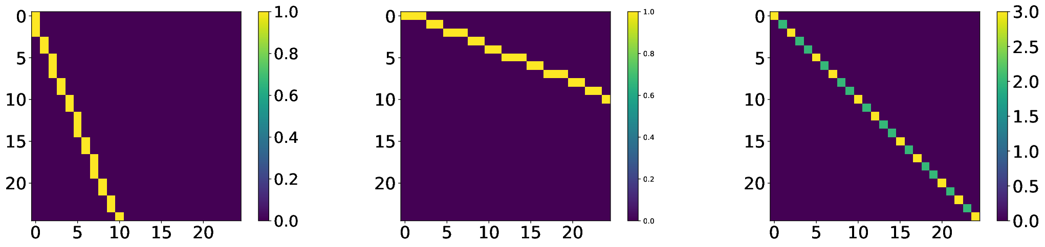
The $\bm{\Theta}_{i}$ matrices are defined by considering $\mathcal{T}$ knots equidistantly distributed in the interval $[1,N_{i}]$ and assigning

with $j=1,\ldots,N_{i}-1$, $k=1,\ldots,\mathcal{T}$ and $\mathcal{T}\geq\max_{i}\left\{N_{i}\right\}$. With this choice, the corresponding Gramian matrices $\bm{G}_{i}$, are diagonal matrices (Fig. 2),

with $\bm{g}_{i}\in\mathbb{R}^{N_{i}}$ and $\bm{1}_{\mathcal{T}}\in\mathbb{R}^{\mathcal{T}}$. Therefore, $\bm{G}_{i}$ is invertible and the back transformation from the phase to the time domain is given by $\bm{\Psi}_{i}=\bm{G}_{i}^{-1}\bm{\Theta}^{T}_{i}$.

From (1) and (2), the ECG beats satisfy $\bm{\xi}_{i}=\bm{\varsigma}_{i}+\bm{\eta}_{i}$. As shown in Fig. 1, in the phase domain the beats have been normalized in lengths and the R-peaks are aligned. Therefore, the phase-domain sample variations are only due to the stochastic inter-beat variations of the ECG beats and noise. As our working model, we assume that the phase domain beats $\bm{\xi}_{i}$ to be ensembles of an underlying $\mathcal{G}\mathcal{P}$

Moreover, from the time domain noise assumption and (2), the phase domain noise beats also have a zero-mean normal distribution $\bm{\eta}_{i}\sim\mathcal{N}\left(\bm{0},v_{n}\bm{\Theta}_{i}\bm{\Theta}_{i}^{T}\right)$. Therefore, the phase domain ECG beats follow $\bm{\varsigma}_{i}\sim\mathcal{N}\left(\bm{\mu}_{\xi},\bm{K}_{\xi}-v_{n}\bm{\Theta}_{i}\bm{\Theta}_{i}^{T}\right)$, where the model parameters $\bm{\mu}_{\xi}$ and $\bm{K}_{\xi}$ can be estimated by the sample mean $\bar{\bm{\mu}}_{\xi}:=B^{-1}\sum_{i=1}^{B}\bm{\xi}_{i}$ and the sample covariance $\bar{\bm{K}}_{\xi}:=B^{-1}\sum_{i=1}^{B}(\bm{\xi}_{i}-\bar{\bm{\mu}}_{\xi})(\bm{\xi}_{i}-\bar{\bm{\mu}}_{\xi})^{T}$, where $B$ is the number of beats. Therefore, the time domain (clean) ECG beats follow a Normal distribution $\bm{s}_{i}\sim\mathcal{N}\left(\bm{\mu}_{s_{i}},\bm{K}_{s_{i}}\right)$ with parameters

where $\hat{v}_{n}$ represents the noise variance estimate and the covariance matrix corresponding to time domains beats $\bm{x}_{i}$ is given by

Finally, the filtered beats are defined as the time domain posterior mean, using (6) and (7):

In the sequel, we refer to $\bm{\mu}_{s_{i}}$ and $\hat{\bm{s}}_{i}$ as prior-based and posterior-based $\mathcal{G}\mathcal{P}$ filter results.

The direct implementation of the filter in (8) requires the inversion of covariance matrices that typically have huge condition numbers. The matrix inversion can be avoided if we consider the diagonal case of $\bar{\bm{K}_{\xi}}$:

In this case, the corresponding time domain matrices are also diagonal and can be computed via

with $\circ$ and $\oslash$ denoting the Hadamard product and division, respectively (element-wise product and division), $\bm{g}_{i}^{2}:=\bm{g}_{i}\circ\bm{g}_{i}$, the time domain (prior) mean computed via

and the corresponding filter given by

The overall algorithm for $\mathcal{G}\mathcal{P}$ ECG filtering is summarized in Algorithm 1 and is available online in our Git repository [7].

The direct implementation of a $\mathcal{G}\mathcal{P}$ filter (without the hereby proposed phase-domain model) would be as follows [1, 2]:

with the computational complexity $\mathcal{O}(N^{3})$, dominated by the inversion of the measurement covariance matrix $\bm{K}_{x}$. In this approach the model’s hyperparameters are the mean $\bm{\mu}_{\bm{s}}$, the covariance matrix $\bm{K}_{\bm{s}}$) and the noise variance $v_{n}$ (or more generally the noise covariance matrix) and optimizing them via classical methods (e.g. maximum evidence, leave-one-out cross validation, [8, Ch. 5]) adds to the computational complexity. For long ECGs, the application of this model is not possible. Previous research considered the $\mathcal{G}\mathcal{P}$ beat-wise formulation and adopted a model-based approach to confine the structure of the covariance matrices [1, 2], but the choice of the particular model-based mean and kernel function families remains ad-hoc and difficult to justify.

The proposed model infers the $\mathcal{G}\mathcal{P}$ mean and covariance matrix in a data-driven way, based on the sample mean and covariance matrix from the phase domain (6) and (7), and in the diagonal case, Algorithm 1, does not require any inversion. The fundamental assumption allowing the data-driven computation is the assumption that the phase domain beats $\bm{\xi}_{i}$ are ensembles from the same underlying $\mathcal{G}\mathcal{P}$, (5).

The number of phase domain beat samples $\mathcal{T}$ is chosen greater than the longest beat in the time domain; this allows the choice of the transformation and back transformation matrices such that the time-phase-time transition can be done without (transformation) errors. The noise variance $\hat{v}_{n}$ can be computed via maximum evidence or practically from the baseline segment of the ECG beats, where the heart is electrically silent and only the noise is exhibited in the ECG.

The BW is removed via two successively zero-phase first order forward-backward lowpass filters (filtfilt in MATLAB/Python SciPy) with cut-off frequencies set at $f_{c}=$ 5.0 Hz and $f_{c}=$ 80.0 Hz, respectively. While the resulting passband frequency range is rather narrow and eliminates some ECG-related components, it enables us to assess the filtering performance for the dominant ECG frequency band.

The proposed filter requires the ECG R-peaks. The beats are defined relative to the R-peaks, segmenting the measurements at the midpoints between successive R-peaks. The R-peak estimation is done using a modified version of the Pan–Tompkins algorithm [9]. Specifically, the version used in this paper estimates the R-peaks by successively applying a band pass filter, an outlier saturation filter via the hyperbolic tangent function, a square root moving average filter and a thresholding.

The PhysioNet QT Database (QTDB) [6] is used to evaluate the developed filter. QTDB consists of 15 minutes 2-lead ECGs sampled at $f_{s}=$ 250 Hz. The baseline wander was removed as detailed in Section III-B. The required software for preprocessing and R-peak detection were adopted from the Open-Source Electrophysiological Toolbox (OSET) [10].

The benchmark filter is a wavelet denoiser with a Symlet–5 mother wavelet, soft thresholding, Stein’s unbiased risk estimate (SURE) shrinkage rule, rescaling using a single-level noise level estimation and four levels of decomposition. In a previous study, this combination was proved to outperform other ECG filtering schemes [3]. The filter evaluation is measured in terms of SNR improvement and QT-interval estimation error.

The ECG records were contaminated by additive white Gaussian noise at SNR levels ranging from –5 to 30 dB, in 5 dB steps. An example of the noisy and filtered ECG are shown in Fig. 3. The average and standard deviation of the SNR improvement is reported for each noise level, for the proposed and benchmark methods in Fig. 4. Accordingly, the proposed posterior-based filter improves the SNR for every level of noise tested and outperforms the prior-based and the benchmark filter for all tested levels of noise.

The accuracy of QT-interval estimation is considered to test the quality of the proposed methods for clinical ECG parameters. For this, the QT-interval estimation error ($\Delta$QT) between the QT-interval estimated from the filtered ECG and the QT-interval estimated from the noiseless ECG is measured and compared between the benchmark and the proposed method at variable input noise levels. The QT-interval estimation method used is adopted from [11]. Fig. 5 shows the median and the interquartile range (IQR) of $\Delta$QT for the benchmark wavelet and the proposed filter, measured over QTDB. Accordingly, compared with the benchmark method, the $\mathcal{G}\mathcal{P}$ posterior filter is reducing the median error for all levels of input noise.

References

- [1] B. Rivet, M. Niknazar, and C. Jutten, “Non parametric modelling of ECG: Applications to denoising and single sensor fetal ECG extraction,” in LVA/ICA 2012 - 10th International Conference on Latent Variable Analysis and Signal Separation, vol. LNCS 7191. Tel-Aviv, Israel: Springer, Mar 2012, pp. 470–477.
- [2] M. Niknazar, B. Rivet, and C. Jutten, “Fetal ECG extraction from a single sensor by a non-parametric modeling,” in 2012 Proceedings of the 20th European Signal Processing Conference, 2012, pp. 949–953.
- [3] R. Sameni, “Online filtering using piecewise smoothness priors: Application to normal and abnormal electrocardiogram denoising,” Signal Processing, vol. 133, pp. 52–63, Apr. 2017. [Online]. Available: https://doi.org/10.1016/j.sigpro.2016.10.019
- [4] P. Laguna, R. Jane, O. Meste, P. Poon, P. Caminal, H. Rix, and N. Thakor, “Adaptive filter for event-related bioelectric signals using an impulse correlated reference input: comparison with signal averaging techniques,” IEEE Transactions on Biomedical Engineering, vol. 39, no. 10, pp. 1032–1044, 1992.
- [5] R. Sameni, M. B. Shamsollahi, C. Jutten, and G. D. Clifford, “A nonlinear bayesian filtering framework for ECG denoising,” Biomedical Engineering, IEEE Transactions on, vol. 54, no. 12, pp. 2172–2185, December 2007. [Online]. Available: https://doi.org/10.1109/TBME.2007.897817
- [6] P. Laguna, R. Mark, A. Goldberg, and G. Moody, “A database for evaluation of algorithms for measurement of QT and other waveform intervals in the ECG,” in Computers in Cardiology 1997. IEEE, 1997. [Online]. Available: https://doi.org/10.1109/cic.1997.648140
- [7] M. Dumitru, Data Driven Gaussian Process filter for ECG, 2022. [Online]. Available: https://github.com/alphanumericslab/OSET/tree/master/UnderDevelopment/DataDrivenGPFilter
- [8] C. E. Rasmussen and C. K. I. Williams, Gaussian Processes for Machine Learning, ser. Adaptive computation and machine learning. The MIT Press, 2005.
- [9] J. Pan and W. J. Tompkins, “A Real-Time QRS Detection Algorithm,” Biomedical Engineering, IEEE Transactions on, vol. BME-32, no. 3, pp. 230–236, 1985.
- [10] R. Sameni, The Open-Source Electrophysiological Toolbox (OSET), version 3.14, 2018. [Online]. Available: https://github.com/alphanumericslab/OSET
- [11] Q. Li, M. Dumitru, and E.A. Perez Alday, et al., “QT-Interval Estimation Improved with Fusion of Multiple Automated Algorithms,” in International Society for Computerized Electrocardiology (ISCE), April 6-10, 2022, Las Vegas, NV, 2022.