跳到论文正文
W Papers独立论文阅读器 arXiv:2301.02543 论文正文 计算阅读时间 · 0%
引用这篇论文根据当前论文元数据生成,正式投稿前建议核对。


License: arXiv.org perpetual non-exclusive license
arXiv:2301.02543v1 [cs.GT] 05 Jan 2023

Zero-Determinant Strategy in Stochastic Stackelberg Asymmetric Security GamePreprint: APS/123-QED

Zhaoyang Cheng Thanks: chengzhaoyang@amss.ac.cn Affiliation:  Key Laboratory of Systems and Control, Academy of Mathematics and Systems Science, Beijing, 100190, China
School of Mathematical Sciences, University of Chinese Academy of Sciences,Beijing, 100049, China
   Guanpu Chen Thanks: chengp@amss.ac.cn Affiliation:  JD Explore Academy, JD.com Inc, Beijing, 100176, China    Yiguang Hong Thanks: yghong@iss.ac.cn Affiliation:  Department of Control Science and Engineering, Tongji University, Shanghai, 201804, China
Shanghai Research Institute for Intelligent Autonomous Systems, Tongji University, Shanghai, 210201, China
Abstract

In a stochastic Stackelberg asymmetric security game, the strong Stackelberg equilibrium (SSE) strategy is a popular option for the defender to get the highest utility against an attacker with the best response (BR) strategy. However, the attacker may be a boundedly rational player, who adopts a combination of the BR strategy and a fixed stubborn one. In such a condition, the SSE strategy may not maintain the defensive performance due to the stubborn element. In this paper, we focus on how the defender can adopt the unilateral-control zero-determinate (ZD) strategy to confront the boundedly rational attacker. At first, we verify the existence of ZD strategies for the defender. We then investigate the performance of the defender’s ZD strategy against a boundedly rational attacker, with a comparison of the SSE strategy. Specifically, when the attacker’s strategy is close to the BR strategy, the ZD strategy admits a bounded loss for the defender compared with the SSE strategy. Conversely, when the attacker’s strategy is close to the stubborn strategy, the ZD strategy can bring higher defensive performance for the defender than the SSE strategy does.

I Introduction

Stochastic security games attract more and more attention in many fields such as the cyber-physical system (CPS), the unmanned aerial vehicle (UAV), and the moving target defense (MTD) Xiao et al. 2018; Feng et al. 2017; Bondi et al. 2020; Mutzari et al. 2021. The stochastic Stackelberg asymmetric security game is one of the important categories to characterize players’ behaviors when the defender faces persistent threats from the attacker. As a fundamental model discussed in Vorobeychik and Singh 2012; Korzhyk et al. 2011, the attacker tends to choose the best response (BR) strategy after observing the defender’ strategy, while the defender aims to maximize its utility considering the attacker. Actually, the defender, as a leader, has an advantage in guiding the attacker’s decision, and the defender picks the optimal strategy based on predicting the attacker’s BR strategy. The corresponding equilibrium is defined as the strong Stackelberg equilibrium (SSE) Vorobeychik and Singh 2012; Li and Hao 2019; Cheng et al. 2022a.

However, players may not always be completely rational due to subjective or objective factors Simon 1990; Jiang et al. 2013 in practice. As a typical case, a boundedly rational attacker does not strictly adopt the BR strategy in practice. This may result from the limitation of the attacker’s observation, the disturbance of the environment, or the imitative behavior of the attacker. For instance, in MTD problems, the attacker may not directly observe the certain defense strategy because of the disturbance from the administrator (defender) Feng et al. 2017; Carvalho and Ford 2014. In UAV systems, the malicious UAV may not observe the location or the flight attitude of the legitimate UAV (defender) due to the obstruction in the wild Bondi et al. 2020. In CPS, the attacker may design a stealthy attack scheme instead of the BR strategy to avoid the fault detection of the defender Xiao et al. 2018; Chen et al. 2021.

When a boundedly rational attacker loses the ability or interest to achieve the BR strategy, it may likely turn to a fixed stubborn strategy in most cases. For example, a player prefers a stubborn strategy to avoid being induced to an unsatisfactory outcome in the CPS security La et al. 2016 and may choose a fixed credible strategy when the player cannot calculate the BR strategy timely in MTD problems Nayak et al. 2016. Against a stubborn attacker, the SSE strategy fails to be regarded as the optimal solution for the defender. In fact, a boundedly rational attacker may choose a mixed strategy, composed by the BR strategy and the stubborn strategy, and such boundedly rational players are common in security problems. For instance, in CPS, the attacker is hesitating between adopting a stubborn strategy or moving as a follower since it needs to consider the failure probability of its own data acquisition system to avoid potential loss Sanjab and Saad 2016. In UAV security problems, a UAV also faces different choices in different stages, since the UAV may lose the location of the defender when going through some complex terrains like in the forest, but fully observes the defender on plains Bondi et al. 2020. Thus, various factors, including the potential preference, inherent cognition, and available resources, make the boundedly rational attacker nonnegligible to the defender.

Clearly, due to the stubborn element within a boundedly rational attacker, the original SSE strategy may be no longer suitable for the defender. Thus, it is important to consider other strategies to help the defender maintain its defensive performance. Fortunately, zero-determinate (ZD) strategies provide a powerful idea to unilaterally enforce an advantageous relation between players’ expected utilities, no matter what strategy the opponent selects. Proposed by Press and Dyson 2012 in iterated prisoner’s dilemma (IPD), a ZD strategy means that one player can unilaterally enforce the two players’ expected utilities subjected to a linear relation. Afterward, various ZD strategies have been widely studied to promote cooperation or unilaterally extortion in public goods games (PGG), human-computer interaction (HCI), evolutionary games, etc Wang et al. 2016; Hilbe et al. 2013; Govaert and Cao 2021; Hao et al. 2015; Engel and Feigel 2018; Szolnoki and Perc 2014; Chen et al. 2022.

Besides, asymmetric matrix games are more realistic than symmetric ones, and there are some challenges to solve the asymmetric games due to the different preferences Taha and Ghoneim 2020; McAvoy and Hauert 2015. Currently, there are not many breakthroughs by applying ZD strategies in symmetric games. For example, some works adopt the ZD strategies to persuade the service provider to cooperate in iterated data trading dilemma games Sooksatra et al. 2018 and to deploy as special active defense strategies in IoT devices Wang et al. 2019. Considering the universality and importance of asymmetric games in security, it is necessary to explore the performance of ZD strategies in asymmetric games under security scenarios, since the original analysis of ZD strategies in IPD cannot be directly applied to the asymmetric security game.

In this paper, we are inspired to reveal whether the defender can adopt the ZD strategy against a boundedly rational attacker in stochastic Stackelberg asymmetric security games, in order to make up for SSE strategies’ deficiencies. To this end, we show that the ZD strategy gives a better performance than the SSE strategy does. The main contribution of this work is summarized as follows.

  • •

    We apply ZD strategies in asymmetric security games. We verify the existence of ZD strategies, in order to ensure the availability of the defender to adopt a ZD strategy. Besides, against the two special attackers, we investigate the defensive performance of ZD strategies compared with SSE strategies. Specifically, against an attacker with the BR strategy, the ZD strategy admits a bounded loss in the utility compared with the SSE strategy, while against a stubborn attacker, the ZD strategy performs well and brings the defender a higher utility than the SSE strategy does.

  • •

    We further analyze a general case where the boundedly rational attacker adopts mixed strategies. The extension takes on analogous tolerable results. When the attacker’s strategy is close to the BR strategy, we provide the defender with appropriate ZD strategies to maintain a bounded loss in defensive performance compared with the SSE strategy, and save the computing resources. Also, when the attacker is close to a stubborn attacker, we show suitable ZD strategies for the defender to get higher defensive performance than SSE strategies.

  • •

    We verify our results in two experiments by providing the defender with proper ZD strategies to compare with an SSE strategy Vorobeychik and Singh 2012. First, we show its performance in MTD problems, where the boundedly rational attacker can directly observe the defender’s strategy and derive its explicit BR strategy Feng et al. 2017; Carvalho and Ford 2014. Then we show its performance in CPS problems. The setting is more complicated but practical than the considered MTD problems, where the attacker can only observe players’ action history and calculate the BR strategy based on certain mechanisms, like the fictitious play and the Q-learning Qiu et al. 2021; Li and Hao 2019.

II Stochastic Stackelberg Asymmetric Security Game

It is known that, in a stochastic asymmetric security game with the memory of the last stage, an attacker aims to invade two targets and a defender prevents the attack in each stage Guo et al. 2019; Feng et al. 2017. Consider the stochastic Stackelberg asymmetric security game 𝒢={𝒮,N,𝒟,𝒜,r,P}\mathcal{G}=\{\mathcal{S},N,\mathcal{D},\mathcal{A},r,P\}. 𝒮={11,12,21,22}\mathcal{S}=\{11,12,21,22\} is the set of states, which is composed by the previous attack and defense targets. N={d,a}N=\{d,a\} is the set of players. 𝒟={1,2}\mathcal{D}=\{1,2\} and 𝒜={1,2}\mathcal{A}=\{1,2\} are the defender’s action set and the attacker’s action set, respectively. 𝐫={rd,ra}\mathbf{r}=\{r_{d},r_{a}\} is the reward set of players, where ri:𝒟×𝒜→ℝr_{i}:\mathcal{D}\times\mathcal{A}\to\mathbb{R}, i∈Ni\in N. Besides, P:𝒮×𝒮×𝒟×𝒜→[0,1]P:\mathcal{S}\times\mathcal{S\times\mathcal{D}\times\mathcal{A}}\to[0,1] is the transition function, where P⁡(s′|s,d,a)P(s^{\prime}|s,d,a) shows the probability to the next state s′∈𝒮s^{\prime}\in\mathcal{S} from the current state ss when players take d,ad,a, and ∑s′∈𝒮P⁡(s′|s,d,a)=1\sum\limits_{s^{\prime}\in\mathcal{S}}P(s^{\prime}|s,d,a)=1 for s∈𝒮,d∈𝒟s\in\mathcal{S},d\in\mathcal{D}, and a∈𝒜a\in\mathcal{A}.

In this security game, since the state presents for the previous players’ actions, P⁡(s′|s,d,a)=1P(s^{\prime}|s,d,a)=1 if and only if s′=(d​a)s^{\prime}=(da) for any s∈𝒮s\in\mathcal{S}. Thus, the next state depends on players’ strategies and the current state. For convenience, denote P⁡(s′|s)P(s^{\prime}|s) as the state transition probability to state s′s^{\prime} from state ss, where s′,s∈𝒮s^{\prime},s\in\mathcal{S}. Furthermore, in the game 𝒢\mathcal{G}, each player’s strategy depends on the current state, which is also a memory-one strategy. The strategy of the defender is a probability distribution πd\pi_{d}, where πd​(d|s)∈Δ​𝒟\pi_{d}(d|s)\in\Delta\mathcal{D} with Δ​𝒟\Delta\mathcal{D} denoting a probability simplex defined on the space 𝒟\mathcal{D}. Similarly, the strategy of the attacker is πa\pi_{a} with πa​(a|s)∈Δ​𝒜\pi_{a}(a|s)\in\Delta\mathcal{A}. Thus, P⁡(s,s′)=πd​(d|s)​πa​(a|s)P(s,s^{\prime})=\pi_{d}(d|s)\pi_{a}(a|s), where s′=(d​a)s^{\prime}=(da). Set M={P⁡(s|s′)}s,s′∈𝒮M=\{P(s|s^{\prime})\}_{s,s^{\prime}\in\mathcal{S}} as the state transition matrix of this security game. As discussed in Akin 2016; Press and Dyson 2012, we carry forward the investigation with a regular matrix MM.

Table 1: Utility matrix
Attacker
1 2
Defender 1 (U11d,U11a)(U^{d}_{11},U^{a}_{11}) (U12d,U12a)(U^{d}_{12},U^{a}_{12})
2 (U21d,U21a)(U^{d}_{21},U^{a}_{21}) (U22d,U22a)(U^{d}_{22},U^{a}_{22})

At stage tt in 𝒢\mathcal{G}, each player observes the current state sts_{t}, and adopts an action according to its strategy. The defender chooses an action dt∈𝒟d_{t}\in\mathcal{D}, while the attacker chooses an action at∈𝒜a_{t}\in\mathcal{A}. The reward of the the defender in stage tt is denoted by rd​(dt,at)=Udt​atdr_{d}(d_{t},a_{t})=U^{d}_{d_{t}a_{t}}, where Udt​atdU^{d}_{d_{t}a_{t}} is the defender’s utility when the defender protects target dtd_{t} and the attacker invades target ata_{t}. Similarly, the reward of the attacker in stage tt is denoted by ra​(dt,at)=Udt​atar_{a}(d_{t},a_{t})=U^{a}_{d_{t}a_{t}}. The utility martix in each stage is shown Table 1.

The expected long-term utilities in the repeated security game are denoted by

Ud​(πd,πa)\displaystyle U_{d}(\pi_{d},\pi_{a}) =𝔼⁡(limT→∞∑t=0Trd​(dt,at)T),\displaystyle=\mathbb{E}\left(\lim_{T\to\infty}\sum\limits_{t=0}^{T}\frac{r_{d}(d_{t},a_{t})}{T}\right),
Ua​(πd,πa)\displaystyle U_{a}(\pi_{d},\pi_{a}) =𝔼⁡(limT→∞∑t=0Tra​(dt,at)T),\displaystyle=\mathbb{E}\left(\lim_{T\to\infty}\sum\limits_{t=0}^{T}\frac{r_{a}(d_{t},a_{t})}{T}\right),

where {dt∼πd(⋅|st)}t⩾0\left\{d_{t}\sim\pi_{d}(\cdot|s_{t})\right\}_{t\geqslant 0}, {at∼πa(⋅|st)}t⩾0\left\{a_{t}\sim\pi_{a}(\cdot|s_{t})\right\}_{t\geqslant 0}, and {st∼P(⋅|st−1,dt−1,at−1)}t>0\left\{s_{t}\sim P(\cdot|s_{t-1},d_{t-1},a_{t-1})\right\}_{t>0} describe the evolution of states and actions over stage. Additionally, s0s_{0} is the initial state ramdomly samplied from 𝒮\mathcal{S}, and the expected utility of each player is the same for any s0s_{0} since MM is convergent.

Assumption 1

The utilities satisfy min⁡{U11d,U22d}>max⁡{U12d,U21d}\min\{U_{11}^{d},U_{22}^{d}\}>\max\{U_{12}^{d},U_{21}^{d}\}. Moreover, U11a<U12aU_{11}^{a}<U_{12}^{a}, and U22a<U21aU_{22}^{a}<U_{21}^{a}.

Different from IPD Press and Dyson 2012; Mamiya and Ichinose 2020, the asymmetry in this security game comes from the actual security mechanism. Specifically, the defender tends to resist attacks, that is, to protect the vulnerable target, and the attacker tends to implement invasions on the unprotected target. The above represents a wide class of asymmetric game in security scenarios, which is summarized as Assumption 1. Similar investigations have been broadly discussed in the literature of various security games Korzhyk et al. 2011; Nguyen and Xu 2019; Guo et al. 2017.

III Boundedly Rational Attacker

In the stochastic Stackelberg asymmetric security game, the defender is a leader and declares a strategy in advance, while the attacker is a follower and chooses its strategy after observing the defender’s strategy. In most cases, the attacker may choose the BR strategy when it obtains the defender’s strategy.

After observing the defender’s strategy πd\pi_{d}, the attacker may choose the BR strategy Li and Hao 2019 as follows:

πaB​R​(πd)∈BR​(πd)=argmaxπa∈Δ​ℬ⁡Ua​(πd,πa).\pi_{a}^{BR}(\pi_{d})\in\textbf{{BR}}(\pi_{d})=\mathop{\text{argmax}}\limits_{\pi_{a}\in\Delta\mathcal{B}}U_{a}(\pi_{d},\pi_{a}).

Without loss of generality, the follower can break ties optimally for the leader if there are multiple options. In this case, the defender aims to maximize its utility considering the attacker, and the equilibrium is defined as the strong Stackelberg equilibrium (SSE) Vorobeychik and Singh 2012; Li and Hao 2019; Cheng et al. 2022a.

Definition 1

A strategy profile (πdS​S​E,πaS​S​E)(\pi_{d}^{SSE},\pi_{a}^{SSE}) is said to be a SSE of 𝒢\mathcal{G} if

(πdS​S​E,πaS​S​E)∈​a​r​g​m​a​xπd,πa∈BR​(πd)⁡Ud​(πd,πa).\displaystyle(\pi_{d}^{SSE},\pi_{a}^{SSE})\in\mathop{\emph{argmax}}\limits_{\pi_{d},\pi_{a}\in{\textbf{\emph{BR}}}({\pi_{d}})}U_{d}(\pi_{d},\pi_{a}).

When the attacker chooses the BR strategy after observing the defender’s strategy, the SSE strategy πdS​S​E\pi_{d}^{SSE} is optimal for the defender, and the defender has an advantage in guiding the attacker’s strategy decision. Besides, if the attacker only observes players’ action history instead of the defender’s strategy directly, the attacker can also choose the BR strategy by some methods such as the fictitious play and the Q-learning method Qiu et al. 2021; Li and Hao 2019.

However, the attacker may not always choose the BR strategy in security problems, due to subjective or objective factors such as the limitation of the attacker’s observation, the disturbance of the environment, and the imitative behavior of the attacker Xiao et al. 2018; Feng et al. 2017; Carvalho and Ford 2014. In practice, the attacker may turn to other strategies. A fixed stubborn strategy, which is not influenced by the defender, is one of the most likely options for the attacker due to its potential preference, inherent cognition, and available resources La et al. 2016; Nayak et al. 2016.

Denote the stubborn strategy in this security game by πa∗\pi_{a}^{*}, while the corresponding attacker is actually a stubborn player. In fact, the attacker intends to keep its action once it finds the most attractive target. For instance, in MTD, there always exists the most vulnerable target for the hacker, and the hacker has no intention to change its attack target once it finds the target Zhuang et al. 2014. Besides, a UAV tends to keep attacking the current optimum target when it has a limited vision and lacks resources to detect others Shan and Zhuang 2018. Without loss of generality, we consider that there exists a target which is more attractive than the other for the attacker, and summarize the above in the following assumption, which was also broadly considered in La et al. 2016; Zhuang et al. 2014; Shan and Zhuang 2018.

Assumption 2

Target 11 is more attractive than target 22 for the attacker, i.e., πa∗​(1|11)=πa∗​(1|21)=1\pi_{a}^{*}(1|11)=\pi_{a}^{*}(1|21)=1.

In fact, either the BR strategy or the stubborn strategy may not be the single optimal option for the attacker. The attacker may adopt a mixed strategy composed by both strategies. The attacker, in this case, is actually called a boundedly rational player, and is not unusual in reality. For instance, the attacker may be hesitating between BR strategies and stubborn strategies due to the errors of the data acquisition system in MTD, and data missing in UAV Sanjab and Saad 2016; Bondi et al. 2020; Gal and Ghahramani 2016. Thus, we formulate the mixed strategy as follows.

Γ1={λ∈[0,1]|(UdS​S​E−U12d)​D​(1)​λ4−A​(1−λ)4−B​λ​(1−λ)⩾0},Γ2={λ∈[0,1]|(U12d−UdS​S​E)​D​(1)​λ4+A​(1−λ)4−B​λ​(1−λ)⩾0},\begin{split}&\Gamma_{1}=\{\lambda\in[0,1]|(U_{d}^{SSE}-U_{12}^{d})D(\textbf{1})\lambda^{4}-A(1-\lambda)^{4}-B\lambda(1-\lambda)\geqslant 0\},\\ &\Gamma_{2}=\{\lambda\in[0,1]|(U_{12}^{d}-U_{d}^{SSE})D(\textbf{1})\lambda^{4}+A(1-\lambda)^{4}-B\lambda(1-\lambda)\geqslant 0\},\end{split} (1)
H⁡(πdZ​D,πdS​S​E,πa∗,λ)=(UdS​S​E−U12d)​C​(πdZ​D,πdS​S​E,πa∗,1)​λ4−A​(1−λ)4+B​λ​(1−λ)C⁡(πdZ​D,πdS​S​E,πa∗,λ).\displaystyle H(\pi_{d}^{ZD},\pi_{d}^{SSE},\pi_{a}^{*},\lambda)=\frac{\left(U_{d}^{SSE}-U_{12}^{d}\right)C(\pi_{d}^{ZD},\pi_{d}^{SSE},\pi_{a}^{*},1)\lambda^{4}-A(1-\lambda)^{4}+B\lambda(1-\lambda)}{C(\pi_{d}^{ZD},\pi_{d}^{SSE},\pi_{a}^{*},\lambda)}. (2)
Definition 2

The attacker’s strategy πaλ​(πd,πa∗)\pi_{a}^{\lambda}(\pi_{d},\pi_{a}^{*}) is called a boundedly rational strategy if

πaλ​(πd,πa∗)=λ​πaB​R​(πd)+(1−λ)​πa∗,λ∈[0,1].\pi_{a}^{\lambda}(\pi_{d},\pi_{a}^{*})=\lambda\pi_{a}^{BR}(\pi_{d})+(1-\lambda)\pi_{a}^{*},\lambda\in[0,1].

For the defender’s strategy πd\pi_{d}, we consider that the boundedly rational attacker adopts the BR strategy πaB​R​(πd)∈𝐁𝐑⁡(πd)\pi_{a}^{BR}(\pi_{d})\in\mathbf{BR}(\pi_{d}) with probability λ\lambda and the stubborn strategy πa∗\pi_{a}^{*} with probability 1−λ1-\lambda Żychowski and Mańdziuk 2021; Jiang et al. 2013. Therefore, when the attacker selects the stubborn strategy, the defender loses the advantage in guiding the attacker’s strategy decision, and the SSE strategy may not maintain the defensive performance due to the stubborn elements therein. Thus, the SSE strategy is no longer suitable for the defender against a boundedly rational attacker. It is important to study other strategies to help the defender maintain its defensive performance.

IV Performance of ZD Strategy

In this section, we introduce the ZD strategy for the defender in the stochastic Stackelberg asymmetric security game. At first, we show the definition of the ZD strategy for the defender and analyze the existence of the ZD strategy. Besides, we explore the performance of the ZD strategy compared with the SSE strategy.

IV.1 ZD Strategy for the Defender

Proposed by Press and Dyson 2012, ZD strategies mean that one player can unilaterally enforce the two players’ expected utilities subjected to a linear relation, which have been widely studied to promote cooperation or unilaterally extortion in public goods game (PGG), human-computer interaction (HCI), and evolutionary games Wang et al. 2016; Hilbe et al. 2013; Govaert and Cao 2021; Hao et al. 2015. For this stochastic Stackelberg asymmetric security game GG, the defender’s ZD strategy Feng et al. 2017; Press and Dyson 2012; Mamiya and Ichinose 2020 is defined as follows:

Definition 3

The defender’s strategy πdZ​D\pi_{d}^{ZD} is called a ZD strategy if

πdZ​D​(1)\displaystyle\pi_{d}^{ZD}(1) =η​𝐒d+β​𝐒a+γ​𝟏4+π^,\displaystyle=\eta\mathbf{S}^{d}+\beta\mathbf{S}^{a}+\gamma\mathbf{1}_{4}+\hat{\pi}, (3)
πdZ​D​(2)\displaystyle\pi_{d}^{ZD}(2) =1−πdZ​D​(1),\displaystyle=1-\pi^{ZD}_{d}(1),

where η,β,γ∈ℝ\eta,\beta,\gamma\in\mathbb{R} and π^=[1,1,0,0]T\hat{\pi}=[1,1,0,0]^{T}.

Let πdZ​D​(k)=[πd​(k|11),πd​(k|12),πd​(k|21),πd​(k|22)]T,\pi_{d}^{ZD}\!(k)\!\!\!=\!\!\![\pi_{d}(\!k|11),\!\pi_{d}(\!k|12),\!\pi_{d}(\!k|21),\!\pi_{d}(\!k|22)]^{T}\!, k∈1,2k\in 1,2 and 𝐒l=[U11l,U12l,U21l,U22l]T\mathbf{S}^{l}=[U^{l}_{11},U^{l}_{12},U^{l}_{21},U^{l}_{22}]^{T}, l∈{d,a}l\in\{d,a\}. The defender’s all feasible ZD strategies are denoted as the following set

Ξ={πZ​Dd∈Δ𝒜|\displaystyle\Xi=\{\pi^{ZD}_{d}\in\Delta\mathcal{A}| πdZ​D​(1)=η​𝐒d+β​𝐒a+γ​𝟏4+π^,\displaystyle\pi^{ZD}_{d}(1)=\eta\mathbf{S}^{d}+\beta\mathbf{S}^{a}+\gamma\mathbf{1}_{4}+\hat{\pi},
πdZ​D(2)=1−πdZ​D(1),η,β,γ∈ℝ}.\displaystyle\pi_{d}^{ZD}(2)=1-\pi_{d}^{ZD}(1),\eta,\beta,\gamma\in\mathbb{R}\}.

It is called zero-determinant (ZD) that, if the defender adopts the ZD strategy with (3), then players’ expected utilities are subjected to a linear relation:

η​Ud​(πdZ​D,πa)+β​Ua​(πdZ​D,πa)+γ=0,∀πa∈Δ​ℬ.\eta U_{d}(\pi_{d}^{ZD},\pi_{a})+\beta U_{a}(\pi_{d}^{ZD},\pi_{a})+\gamma=0,\ \forall\pi_{a}\in\Delta\mathcal{B}.

Take πZ​D​(η,β,γ)\pi^{ZD}(\eta,\beta,\gamma) as the corresponding ZD strategy. With the help of the ZD strategy’s unilateral enforcement in players’ utilities, we aim to investigate whether the defender can adopt the ZD strategy to better maintain its defensive performance than the original SSE strategy against a boundedly rational attacker.

In what follows, we investigate the existence of ZD strategies to guarantee the availability for the defender.

IV.2 Existence of ZD Strategy

Actually, the ZD strategy cannot enforce an arbitrary linear relation between two players’ utilities since it must belong to the implementer’s strategy set. Thus, a feasible linear relation enforced by ZD strategies is fundamental for further analysis. The following lemma provides a necessary and sufficient condition for the feasibility of a linear relationship between players’ utilities, whose proof can be found in Appendix B.

Lemma 1

Under Assumption 1, there exists a ZD strategy which enforces η​Ud+β​Ua+γ=0\eta U_{d}+\beta U_{a}+\gamma=0 if and only if either of the following two inequalities is satisfied.

maxs∈{11,12}⁡η​Usd+β​Usa⩽−γ⩽mins∈{21,22}⁡η​Usd+β​Usa.\max\limits_{s\in\{11,12\}}\eta U_{s}^{d}+\beta U_{s}^{a}\leqslant-\gamma\leqslant\min\limits_{s\in\{21,22\}}\eta U_{s}^{d}+\beta U_{s}^{a}. (4)
maxs∈{21,22}⁡η​Usd+β​Usa⩽−γ⩽mins∈{11,12}⁡η​Usd+β​Usa.\max\limits_{s\in\{21,22\}}\eta U_{s}^{d}+\beta U_{s}^{a}\leqslant-\gamma\leqslant\min\limits_{s\in\{11,12\}}\eta U_{s}^{d}+\beta U_{s}^{a}. (5)

Lemma 1 implies that the defender can adopt the ZD strategy πZ​D​(η,β,γ)\pi^{ZD}(\eta,\beta,\gamma), where η\eta, β\beta, and γ\gamma satisfy (4) or (5), to enforce an ideal linear relation between players’ excepted utilities. Actually, Lemma 1 extends the application of ZD strategies since the payoff matrix in security games is not as symmetric as that in IPD games Hilbe et al. 2015. Moreover, Lemma 1 covers the following cases.

  • •

    The defender can unilaterally restrict attacker’s utility if U11a>U12aU_{11}^{a}>U_{12}^{a}. If the defender takes πZ​D​(η,β,γ)\pi^{ZD}(\eta,\beta,\gamma) with η=0,β≠0\eta=0,\beta\neq 0, and U12a⩽−γβ⩽U11aU_{12}^{a}\leqslant-\frac{\gamma}{\beta}\leqslant U_{11}^{a}, then the defender ZD can unilaterally restrict the attacker’s utility as −γβ∈[U11a,U12a]-\frac{\gamma}{\beta}\in[U_{11}^{a},U_{12}^{a}], which is the same as the equalizer strategy in IPD games Press and Dyson 2012; Cheng et al. 2022b.

  • •

    The defender can unilaterally restrict its own utility if U12d>U22dU_{12}^{d}>U_{22}^{d}. If the defender takes πZ​D​(η,β,γ)\pi^{ZD}(\eta,\beta,\gamma) with η≠0,β=0\eta\neq 0,\beta=0, and U22d⩽−γη⩽U12dU_{22}^{d}\leqslant-\frac{\gamma}{\eta}\leqslant U_{12}^{d}, then the defender can unilaterally restrict the defender’s utility between U22dU_{22}^{d} and U12dU_{12}^{d}, which is consistent with the result in MTD problems Wang et al. 2019.

Based on the existence condition of feasible linear relations enforced by ZD strategies, we can further analyze whether there exists at least one ZD strategy in the security game 𝒢\mathcal{G}. For simplification, for any x1,x2,y1,y2∈ℝx_{1},x_{2},y_{1},y_{2}\in\mathbb{R} with x1≠x2x_{1}\neq x_{2}, denote

Γ−​(x1,y1,x2,y2)={(x,y)|y−y1⩽y2−y1x2−x1​(x−x1)},\displaystyle\Gamma^{-}(x_{1},y_{1},x_{2},y_{2})=\{(x,y)|y-y_{1}\leqslant\frac{y_{2}-y_{1}}{x_{2}-x_{1}}(x-x_{1})\},
Γ+​(x1,y1,x2,y2)={(x,y)|y−y1⩾y2−y1x2−x1​(x−x1)}.\displaystyle\Gamma^{+}(x_{1},y_{1},x_{2},y_{2})=\{(x,y)|y-y_{1}\geqslant\frac{y_{2}-y_{1}}{x_{2}-x_{1}}(x-x_{1})\}.

Actually, Γ−\Gamma^{-} (Γ+\Gamma^{+}) is the region above (below) the line going through points (x1,y1)(x_{1},y_{1}) and (x2,y2)(x_{2},y_{2}). Then the following theorem shows a sufficient condition for the existence of a ZD strategy in 𝒢\mathcal{G}, whose proof can be found in Appendix C.

Theorem 1

Under Assumption 1, there exists at least one ZD strategy of the defender in 𝒢\mathcal{G} if either of the following two relations is satisfied.

(U21d,U21a),(U22d,U22a)∈Γ+​(U11d,U11a,U12d,U12a).\displaystyle(U_{21}^{d},U_{21}^{a}),(U_{22}^{d},U_{22}^{a})\in\Gamma^{+}(U_{11}^{d},U_{11}^{a},U_{12}^{d},U_{12}^{a}).
(U21d,U21a),(U22d,U22a)∈Γ−​(U11d,U11a,U12d,U12a).\displaystyle(U_{21}^{d},U_{21}^{a}),(U_{22}^{d},U_{22}^{a})\in\Gamma^{-}(U_{11}^{d},U_{11}^{a},U_{12}^{d},U_{12}^{a}).
Refer to caption
Figure 1: (U11d,U11a)(U_{11}^{d},U_{11}^{a}) and (U12d,U12a)(U_{12}^{d},U_{12}^{a}) lie in the one side of the line η​Ua+β​Ub+γ=0\eta U_{a}+\beta U_{b}+\gamma=0, while (U21d,U21a)(U_{21}^{d},U_{21}^{a}) and (U22d,U22a)(U_{22}^{d},U_{22}^{a}) lie in the other side.

Theorem 1 shows that, in the security game 𝒢\mathcal{G}, the defender is able to choose a ZD strategy once (U21d,U21a),(U22d,U22a)(U_{21}^{d},U_{21}^{a}),(U_{22}^{d},U_{22}^{a}) lie in the same side of the line going through points (U11d,U11a)(U_{11}^{d},U_{11}^{a}) and (U12d,U12a)(U_{12}^{d},U_{12}^{a}), as shown in Fig 1. Hence, in this paper, we focus on the situation where there exists at least a ZD strategy, since selecting ZD strategies for the defender is based on its existence. In fact, the two conditions are interchangeable. For example, if (U21d,U21a),(U22d,U22a)∈Γ−​(U11d,U11a,U12d,U12a)(U_{21}^{d},U_{21}^{a}),(U_{22}^{d},U_{22}^{a})\in\Gamma^{-}(U_{11}^{d},U_{11}^{a},U_{12}^{d},U_{12}^{a}), then can get (U21d,U21a),(U22d,U22a)∈Γ−​(U11d,U11a,U12d,U12a)(U_{21}^{d},U_{21}^{a}),(U_{22}^{d},U_{22}^{a})\in\Gamma^{-}(U_{11}^{d},U_{11}^{a},U_{12}^{d},U_{12}^{a}) by swaping the values of (U11d,U11a)(U_{11}^{d},U_{11}^{a}) and (U22d,U22a)(U_{22}^{d},U_{22}^{a}), and swaping the values of (U12d,U12a)(U_{12}^{d},U_{12}^{a}) and (U21d,U21a)(U_{21}^{d},U_{21}^{a}). Hence, without loss of generality, the rest results in this paper are established with the condition (U21d,U21a),(U22d,U22a)∈Γ−​(U11d,U11a,U12d,U12a)(U_{21}^{d},U_{21}^{a}),(U_{22}^{d},U_{22}^{a})\in\Gamma^{-}(U_{11}^{d},U_{11}^{a},U_{12}^{d},U_{12}^{a}).

IV.3 ZD Strategy in Two Special Cases

For understanding easily, we start with two special cases: λ=1\lambda=1, where the attacker takes BR strategies Li and Hao 2019, and λ=0\lambda=0, where the attacker is a stubborn player with stubborn strategies La et al. 2016; Nayak et al. 2016.

When 𝝀=𝟏\bm{\lambda=1}, the attacker chooses BR​(πd)\textbf{{BR}}(\pi_{d}) after observing the defender’s strategy πd\pi_{d}. Recall the definition of (πdS​S​E,πaS​S​E)(\pi_{d}^{SSE},\pi_{a}^{SSE}) as a SSE and UdS​S​EU_{d}^{SSE} as the defender’s utility from an SSE strategy.

Lemma 2

Under Assumption 1, for any πdZ​D∈Ξ\pi_{d}^{ZD}\in\Xi and πa∈B​R​(πdZ​D)\pi_{a}\in BR(\pi_{d}^{ZD}), Ud​(πdZ​D,πa)⩽Ud​(πdS​S​E,πaS​S​E)U_{d}(\pi_{d}^{ZD},\pi_{a})\leqslant U_{d}(\pi_{d}^{SSE},\pi_{a}^{SSE}).

Lemma 2 reveals that the SSE strategy always brings the highest utility for the defender when facing an attacker with the BR strategy. In this case, the upper limit of the performance of ZD strategies cannot surpass the defender’s utility with adopting an SSE strategy. In spite of this, the following theorem tells that ZD strategies admit a bounded loss compared with SSE strategies, whose proof can be found in Appendix D.

Refer to caption
(a) Attacker with the BR strategy
Refer to caption
(b) Attacker with the stubborn strategy
Refer to caption
(c) Boundedly Rational Attacker
Figure 2: Performance of the ZD strategy compared with the SSE strategy in MTD problems. Red dotted lines describe the defender’s expected utilities adopting an SSE strategy, while blue solid lines describe them adopting the corresponding ZD strategy. In (c), the red (blue) region shows the bound of Γ1\Gamma_{1} (Γ2\Gamma_{2}) according to Theorem 4 (Theorem 5).
Theorem 2

Under Assumption 1,

minπdZ​D∈Ξ⁡Ud​(πdS​S​E,πaB​R​(πdS​S​E))−Ud​(πdZ​D,πaB​R​(πdZ​D))\displaystyle\min\limits_{\pi_{d}^{ZD}\in\Xi}U_{d}\left(\pi_{d}^{SSE},\pi_{a}^{BR}(\pi_{d}^{SSE})\right)\!-\!U_{d}\left(\pi_{d}^{ZD},\pi_{a}^{BR}(\pi_{d}^{ZD})\right)
={0,if ​U11d⩾U21d,UdS​S​E−U12d,if ​U11d<U21d.\displaystyle=\left\{\begin{array}[]{ll}0,&\quad\quad\quad\text{if }U_{11}^{d}\geqslant U_{21}^{d},\\ U_{d}^{SSE}-U_{12}^{d},&\quad\quad\quad\text{if }U_{11}^{d}<U_{21}^{d}.\end{array}\right.

The corresponding ZD strategy is πdZ​D\pi_{d}^{ZD}

={πZ​D​(−k1,1,k1​U11d−U11a),ifU11d⩾U22d,U11a⩾U21a,πZ​D​(0,1,−U21a),ifU11d<U22d,U11a⩾U21a,πZ​D​(−k2,1,k2​U12d−U12a),otherwise,=\!\!\left\{\begin{array}[]{ll}\pi^{ZD}\!(\!-\!k_{1},\!1,\!k_{1}U_{11}^{d}\!\!-\!U_{11}^{a}\!),&\!\!\text{if}\ U_{11}^{d}\!\geqslant\!U_{22}^{d},\ U_{11}^{a}\!\geqslant\!U_{21}^{a},\\ \pi^{ZD}(0,\!1,\!-U_{21}^{a}),&\!\!\text{if}\ U_{11}^{d}\!<\!U_{22}^{d},\ U_{11}^{a}\!\geqslant\!U_{21}^{a},\\ \pi^{ZD}\!(\!-\!k_{2},\!1,\!k_{2}U_{12}^{d}\!\!-\!U_{12}^{a}\!),&\!\!\text{otherwise,}\end{array}\right.

where 0⩽k1⩽U11a−U21aU11d−U21d0\leqslant k_{1}\leqslant\frac{U_{11}^{a}-U_{21}^{a}}{U_{11}^{d}-U_{21}^{d}}, and U22a−U12aU22d−U12d⩽k2⩽U11a−U12aU11d−U12d\frac{U_{22}^{a}-U_{12}^{a}}{U_{22}^{d}-U_{12}^{d}}\leqslant k_{2}\leqslant\frac{U_{11}^{a}-U_{12}^{a}}{U_{11}^{d}-U_{12}^{d}}.

Theorem 2 shows that the defender can adopt ZD strategies to get an tolerable loss in the utility compared with SSE strategies. On the one hand, when U11a⩾U21aU_{11}^{a}\geqslant U_{21}^{a}, the ZD strategy in Theorem 2 is an SSE strategy and brings the defender the same utility as SSE strategies. On the other hand, if the defender can endure the bounded loss, then adopting the corresponding ZD strategy is also a good choice to avoid the complex calculation for SSE strategies, since deriving SSE strategies needs solve a bi-level optimization problem.

When 𝝀=𝟎\bm{\lambda=0}, the attacker chooses the stubborn strategy πa∗\pi_{a}^{*}. The SSE strategy may not bring the defender a tolerable utility, since the stubborn attacker does not choose the BR strategy as the defender’s expectation. In this case, due to the ZD strategy’s unilateral enforcement in players’ utilities, a ZD strategy can exactly play an essential role to enforce desired utilities for the defender and even to bring a higher utility than the original SSE strategy does, and the following theorem’s proof can be found in Appendix E

Theorem 3

Under Assumptions 1 and 2, there exists a ZD strategy πdZ​D=πZ​D​(−k,1,k​U12d−U12a)\pi_{d}^{ZD}=\pi^{ZD}(-k,1,kU_{12}^{d}-U_{12}^{a}) with k=U11a−U12aU11d−U12dk=\frac{U_{11}^{a}-U_{12}^{a}}{U_{11}^{d}-U_{12}^{d}} such that

Ud​(πdZ​D,πa∗)⩾Ud​(πdS​S​E,πa∗).U_{d}(\pi_{d}^{ZD},\pi_{a}^{*})\geqslant U_{d}(\pi_{d}^{SSE},\pi_{a}^{*}).

In fact, the ZD strategy πZ​D​(−k,1,k​U12d−U12a)\pi^{ZD}(-k,1,kU_{12}^{d}-U_{12}^{a}) enforces the linear relation between players’ expected utilities going through (U12a,U12b)(U_{12}^{a},U_{12}^{b}) and (U11d,U11a)(U_{11}^{d},U_{11}^{a}). The infimum of the ZD strategy πZ​D​(−k,1,k​U12d−U12a)\pi^{ZD}(-k,1,kU_{12}^{d}-U_{12}^{a}) is not lower than that of any other ZD strategy, including the ones which can unilaterally set the defender’s utility Wang et al. 2019. Moreover, according to its proof, when facing the stubborn attacker, this ZD strategy πdZ​D\pi_{d}^{ZD} brings an increase U11d−U11d​πdS​S​E​(1|21)+U21d​πdS​S​E​(2|11)πdS​S​E​(2|11)+πdS​S​E​(1|21)U_{11}^{d}-\frac{U_{11}^{d}\pi_{d}^{SSE}(1|21)+U_{21}^{d}\pi_{d}^{SSE}(2|11)}{\pi_{d}^{SSE}(2|11)+\pi_{d}^{SSE}(1|21)} in utility for the defender compared with the SSE strategy.

IV.4 ZD Strategy in General Case

It is time to consider the general case when 𝝀∈[𝟎,𝟏]\bm{\lambda\in[0,1]}. Here, the boundedly rational attacker chooses the BR strategy with probability λ\lambda and the stubborn strategy πa∗\pi_{a}^{*} with probability 1−λ1-\lambda, i.e., πaλ​(πd,πa∗)\pi_{a}^{\lambda}(\pi_{d},\pi_{a}^{*}) in Definition 2. Intuitively, the ZD strategy may bring the defender a similar performance as shown in Theorem 2 when λ\lambda is close to 11, and a similar performence as given in Theorem 3 when λ\lambda is close to 00. In fact, one main result of this subsection is given in the following theorem, whose proof can be found in Appendix F.
Refer to caption
(a) Fictitious play with λ=0.1\lambda=0.1
Refer to caption
(b) Fictitious play with λ=0.2\lambda=0.2
Refer to caption
(c) Fictitious play with λ=0.8\lambda=0.8
Refer to caption
(d) Fictitious play with λ=0.9\lambda=0.9
Refer to caption
(e) Q-learning with λ=0.1\lambda=0.1
Refer to caption
(f) Q-learning with λ=0.2\lambda=0.2
Refer to caption
(g) Q-learning with λ=0.8\lambda=0.8
Refer to caption
(h) Q-learning with λ=0.9\lambda=0.9
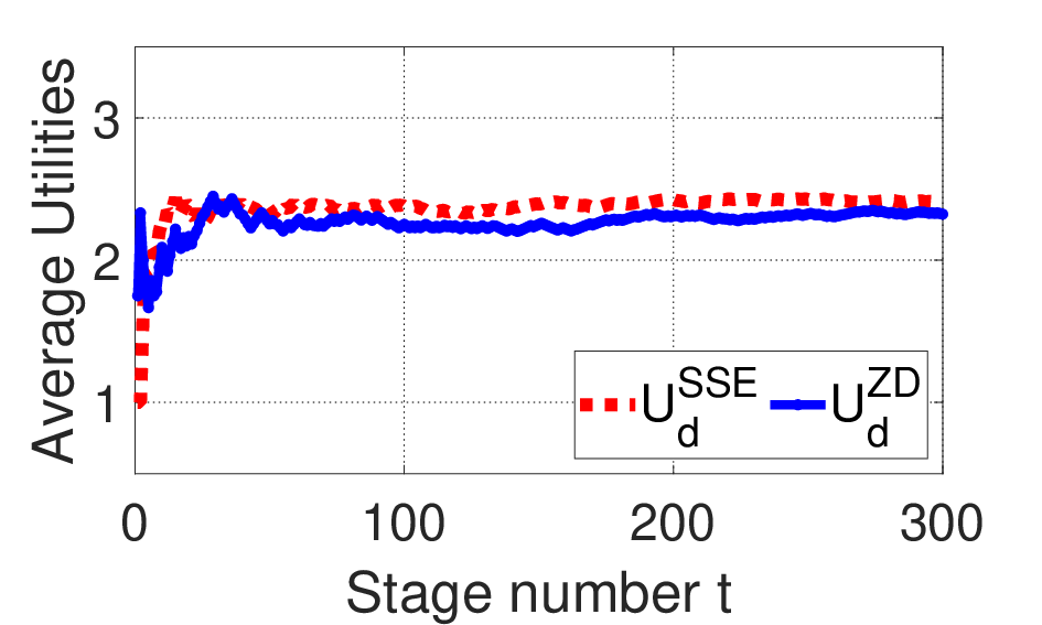
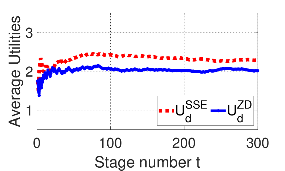
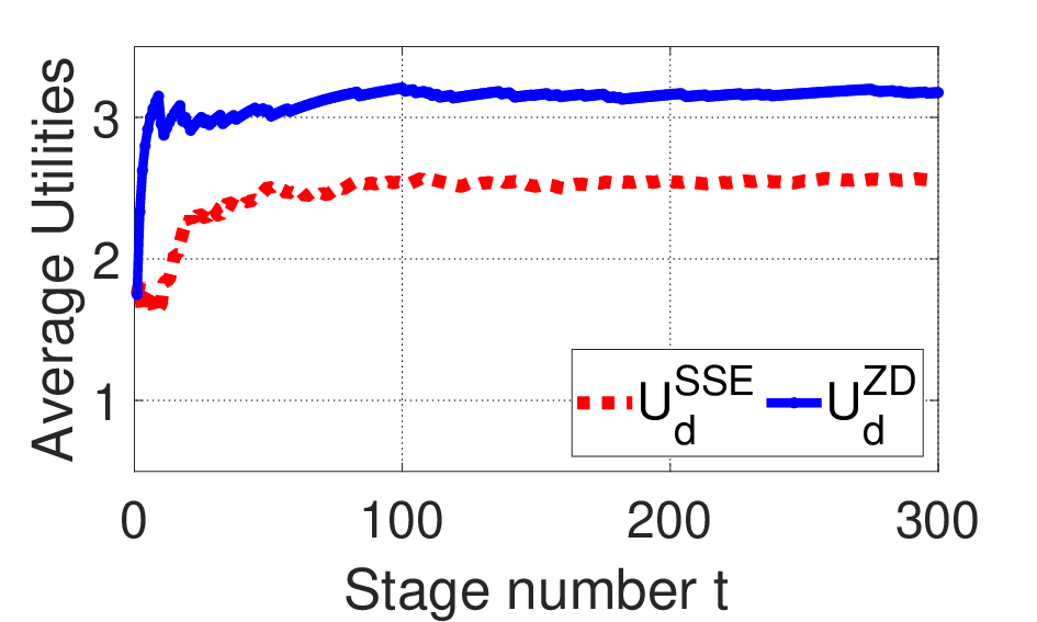
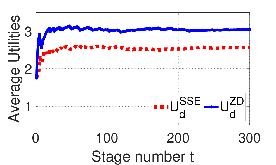
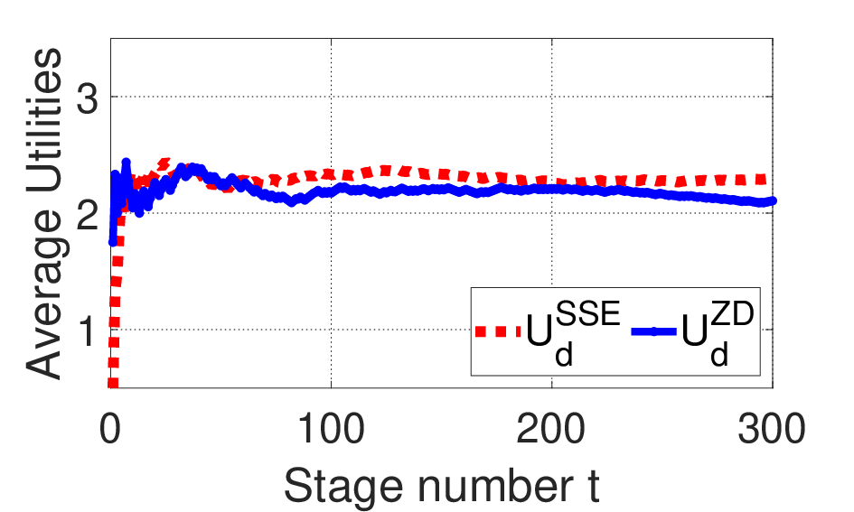
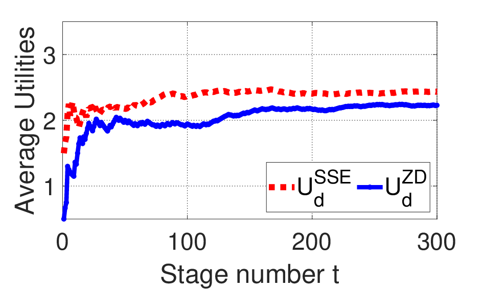
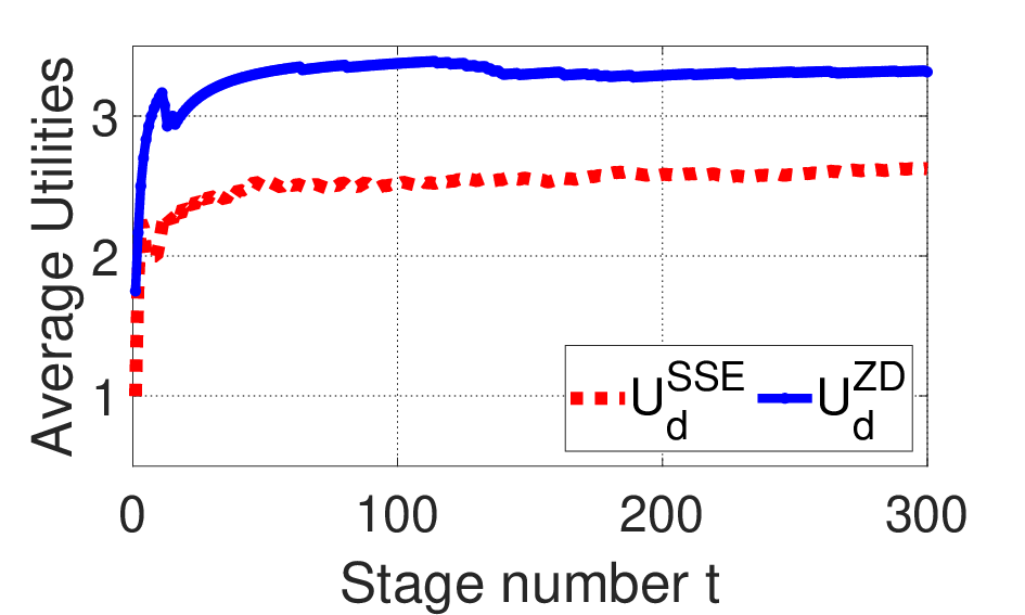
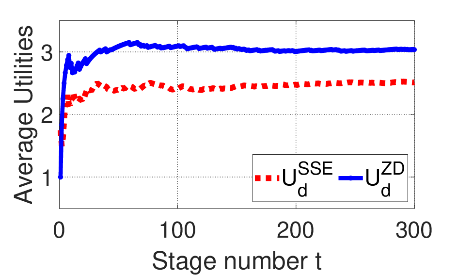
Figure 3: Performance of the ZD strategy compared with the SSE strategy in CPS with different mechanisms. Red dotted lines show the defender’s average utility adopting an SSE strategy, while blue solid lines show the defender’s average utility adopting the corresponding ZD strategy in Theorem 4 or Theorem 5.
Theorem 4

Under Assumptions 1 and 2, for λ∈Γ1\lambda\in\Gamma_{1} in (1), there is

minπdZ​D∈Ξ⁡Ud​(πdS​S​E,πaλ​(πdS​S​E,πa∗))−Ud​(πdZ​D,πaλ​(πdZ​D,πa∗))\displaystyle\min\limits_{\pi_{d}^{ZD}\in\Xi}\!U_{d}\left(\pi_{d}^{SSE}\!,\!\pi_{a}^{\lambda}(\pi_{d}^{SSE}\!,\!\pi_{a}^{*})\!\right)\!-\!U_{d}\left(\pi_{d}^{ZD}\!,\!\pi_{a}^{\lambda}(\pi_{d}^{ZD},\!\pi_{a}^{*})\!\right)
⩽{0,ifU11d⩾U22d,U11a⩾U21a,H⁡(πdZ​D,πdS​S​E,πa∗,λ),otherwise,\displaystyle\leqslant\!\!\left\{\begin{array}[]{ll}0,&\text{if}\ U_{11}^{d}\!\geqslant\!U_{22}^{d},\ U_{11}^{a}\!\geqslant\!U_{21}^{a},\\ H(\pi_{d}^{ZD},\pi_{d}^{SSE},\pi_{a}^{*},\lambda),&\text{otherwise},\end{array}\right.

where H⁡(πdZ​D,πdS​S​E,πa∗,λ)H(\pi_{d}^{ZD},\pi_{d}^{SSE},\pi_{a}^{*},\lambda) was defined in (2), and the parameters therein are shown in Appendix A. The corresponding ZD strategy is πdZ​D\pi_{d}^{ZD}

={πZ​D​(−k1,1,k1​U11d−U11a),ifU11d⩾U22d,U11a⩾U21a,πZ​D​(−k2,1,k2​U12d−U12a),otherwise,=\!\!\left\{\!\begin{array}[]{ll}\!\pi^{ZD}(-k_{1},\!1,\!k_{1}U_{11}^{d}\!-\!U_{11}^{a}),&\text{if}\ U_{11}^{d}\!\geqslant\!U_{22}^{d},\ U_{11}^{a}\!\geqslant\!U_{21}^{a},\\ \!\pi^{ZD}(-k_{2},\!1,\!k_{2}U_{12}^{d}\!-\!U_{12}^{a}),&\text{otherwise},\end{array}\right.

where 0⩽k1⩽U11a−U21aU11d−U21d0\leqslant k_{1}\leqslant\frac{U_{11}^{a}-U_{21}^{a}}{U_{11}^{d}-U_{21}^{d}}, and k2=U11a−U12aU11d−U12dk_{2}=\frac{U_{11}^{a}-U_{12}^{a}}{U_{11}^{d}-U_{12}^{d}}.

Theorem 4 provides the set Γ1\Gamma_{1} for the defender, in which the ZD strategy brings a bounded and tolerable loss in defensive performance, even though the ZD strategy cannot surplus the SSE strategy. Thus, for the boundedly rational attacker with λ∈Γ1\lambda\in\Gamma_{1}, if the defender does not care too much about losing a little utility, then the defender can adopt the corresponding ZD strategy since adopting the ZD strategy in Theorem 4 avoids paying vast resources to solve a bi-level optimization problem for the SSE strategy. Moreover, if U11a⩾U21aU_{11}^{a}\geqslant U_{21}^{a} and U11d⩾U22dU_{11}^{d}\geqslant U_{22}^{d}, the ZD strategy can bring the defender the same utility as an SSE strategy, which means that the defender can still adopt ZD strategies.

Although Γ1\Gamma_{1} seems complicated to verify, some typical value of λ\lambda is easy to be confirmed whether it belongs to Γ1\Gamma_{1}. For instance, λ=1\lambda=1 is always in Γ1\Gamma_{1}. In this case, the attacker tends to take the BR strategy, which is consistent with Theorem 2. Actually, λ\lambda is in Γ1\Gamma_{1} if λ\lambda is close to 11, which means that the attacker tends to choose the BR strategy. Also, we provide a subset of Γ1\Gamma_{1}, which can be verified easily by the defender.

Corollary 1

Under Assumptions 1 and 2, if λ∈[12,1]\lambda\in[\frac{1}{2},1] and

4​(U11d−U21d)​πdS​S​E​(2|11)​(1−λ)4\displaystyle 4(U_{11}^{d}-U_{21}^{d})\pi_{d}^{SSE}(2|11)(1-\lambda)^{4}
⩽\displaystyle\leqslant (14​(UdS​S​E−U12d)​D​(1)−B)​(πdS​S​E​(2|11)+πdS​S​E​(1|21)),\displaystyle\left(\frac{1}{4}(U_{d}^{SSE}\!\!-\!U_{12}^{d})D(\textbf{1})\!-\!B\right)\!\!\left(\pi_{d}^{SSE}(2|11)\!+\!\pi_{d}^{SSE}(1|21)\right),

then

minπdZ​D∈Ξ⁡Ud​(πdS​S​E,πaλ​(πdS​S​E,πa∗))−Ud​(πdZ​D,πaλ​(πdZ​D,πa∗))\displaystyle\min\limits_{\pi_{d}^{ZD}\in\Xi}\!U_{d}\left(\pi_{d}^{SSE}\!,\!\pi_{a}^{\lambda}(\pi_{d}^{SSE}\!,\!\pi_{a}^{*})\!\right)\!-\!U_{d}\left(\pi_{d}^{ZD}\!,\!\pi_{a}^{\lambda}(\pi_{d}^{ZD},\!\pi_{a}^{*})\!\right)
⩽{0,ifU11a⩾U21a,U11d⩾U22d,H⁡(πdZ​D,πdS​S​E,πa∗,λ),otherwise.\displaystyle\leqslant\!\!\left\{\begin{array}[]{ll}0,&\text{if}\ U_{11}^{a}\!\geqslant\!U_{21}^{a},\ U_{11}^{d}\!\geqslant\!U_{22}^{d},\\ H(\pi_{d}^{ZD},\pi_{d}^{SSE},\pi_{a}^{*},\lambda),&\text{otherwise}.\end{array}\right.

At last, we analogously consider the situation when λ\lambda is close to 00, i.e., the attacker tends to take the stubborn strategy in the following theorem, whose proof can be found in Appendix G.

Theorem 5

Under Assumptions 1 and 2, if λ∈Γ2\lambda\in\Gamma_{2} in (1), then there exists a ZD strategy πdZ​D=πZ​D​(−k,1,k​U21a−U21b)\pi_{d}^{ZD}=\pi^{ZD}(-k,1,kU_{21}^{a}-U_{21}^{b}) such that

Ud​(πdZ​D,πaλ​(πdZ​D,πa∗))⩾Ud​(πdS​S​E,πaλ​(πdS​S​E,πa∗)),U_{d}(\pi_{d}^{ZD},\pi_{a}^{\lambda}(\pi_{d}^{ZD},\pi_{a}^{*}))\!\geqslant\!U_{d}(\pi_{d}^{SSE},\pi_{a}^{\lambda}(\pi_{d}^{SSE},\pi_{a}^{*})),

where k=U11b−U12bU11a−U12a.k=\frac{U_{11}^{b}-U_{12}^{b}}{U_{11}^{a}-U_{12}^{a}}.

Theorem 5 provides the set Γ2\Gamma_{2} for the defender to adopt the ZD strategy to get a higher utility than the original SSE strategy. Notice that the corresponding ZD strategy yields wonderful performance. If λ∈Γ2\lambda\in\Gamma_{2}, the defender can confidently select the corresponding ZD strategy, since the ZD strategy brings the defender higher defensive performance than an SSE strategy does.

Clearly, λ=0\lambda=0 is always in Γ2\Gamma_{2}, which is consistent with the results in Theorem 3. Actually, λ\lambda is in Γ2\Gamma_{2} if λ\lambda is close to 00, which means that the attacker tends to be a stubborn attacker. Also, we provide a subset of Γ2\Gamma_{2} for the defender, which can be verified easily by the defender.

Corollary 2

Under Assumptions 1 and 2, if λ∈[0,12]\lambda\in[0,\frac{1}{2}] and

4​(UdS​S​E−U12a)​D​(1)​λ4⩽14​A−B,4(U_{d}^{SSE}-U_{12}^{a})D(\textbf{1})\lambda^{4}\leqslant\frac{1}{4}A-B,

then there exists πdZ​D∈Ξ\pi_{d}^{ZD}\in\Xi such that

Ud​(πdZ​D,πaλ​(πdZ​D,πa∗))⩾Ud​(πdS​S​E,πaλ​(πdS​S​E,πa∗)).U_{d}(\pi_{d}^{ZD},\pi_{a}^{\lambda}(\pi_{d}^{ZD},\pi_{a}^{*}))\!\geqslant\!U_{d}(\pi_{d}^{SSE},\pi_{a}^{\lambda}(\pi_{d}^{SSE},\pi_{a}^{*})).

V Applications

For illustration, we provide experiments to verify that the ZD strategy can help the defender maintain its defensive performance against a boundedly rational attacker, where the baseline is the original SSE strategy.

V.1 In MTD Problems

Let us consider an MTD problem, where the attacker can directly observe the defender’s strategy and take its explicit BR strategy Feng et al. 2017; Carvalho and Ford 2014. Take YiY_{i} as the cost of the defender moving the defense resource from target ii to the other target, and take CiC_{i} as the cost of the attacker invading target ii. Similar to Wang et al. 2019, we also use the average to approximate the transfer cost. Also, take RidR^{d}_{i} and RiaR^{a}_{i} as the reward and loss for two players in the state i∈𝒮i\in\mathcal{S}. Thus, the utility matrix in MTD problems is shown in Table 2. Take Rsd=ds1​θ+ds0R_{s}^{d}=d_{s}^{1}\theta+d_{s}^{0}, and Rsa=as1​θ+as0R_{s}^{a}=a_{s}^{1}\theta+a_{s}^{0} for any s∈𝒮s\in\mathcal{S}, where θ∈[0,1]\theta\in[0,1], and dskd_{s}^{k} and aska_{s}^{k} are parameters in players’ rewards and losses, respectively, for any s∈𝒮s\in\mathcal{S} and k∈{1,2}k\in\{1,2\}.

Table 2: Utility matrix in MTD problems
Attacker
1 2
Defender​ 1 (R11d−Y22,R11a−C1)(R^{d}_{11}\!-\!\frac{Y_{2}}{2},\!R^{a}_{11}\!-\!C_{1}) (R12d−Y22,R12a−C2)(R^{d}_{12}\!-\!\frac{Y_{2}}{2},R^{a}_{12}\!-\!C_{2})
2 (R21d−Y12,R21a−C1)(R^{d}_{21}\!-\!\frac{Y_{1}}{2},\!R^{a}_{21}\!-\!C_{1}) (R22d−Y12,R22a−C2)(R^{d}_{22}\!-\!\frac{Y_{1}}{2},\!R^{a}_{22}\!-\!C_{2})

As shown in Fig 2(a), for an attacker with the BR strategy, the expected utility of the defender with an SSE strategy is always higher than that with a ZD strategy. Besides, in Fig 2(b), for an attacker with the stubborn strategy, the expected utility of the defender with adopting the ZD strategy in Theorem 3 is always higher than that with adopting an SSE strategy. Moreover, in Fig 2(c), UdZ​DU_{d}^{ZD} is always higher than UdS​S​EU_{d}^{SSE} when λ<0.21\lambda<0.21, which is consistent with Theorem 5. Also, UdS​S​EU_{d}^{SSE} is always higher than UdZ​DU_{d}^{ZD} when λ>0.78\lambda>0.78, which is consistent with Theorem 4, and the difference between the two utilities is bounded and tolerable.

V.2 In CPS Problems

Here we consider a CPS problem with a defender as a system administrator and an attacker as a jammer or an eavesdropper. Here, different from the previous experiment, the attacker can only observe players’ action history without directly receiving the defender’s strategy. The attacker adopts the BR strategy based on the fictitious play Qiu et al. 2021 or the Q-learning method Li and Hao 2019, whose details are provided in Appendix H.

As shown in Fig 3(a)-(f), when λ\lambda is close to 00, like 0.10.1 in Fig 3(a), (e), and 0.20.2 in Fig 3(b), (f), the average utility of the defender with the ZD strategy is higher than that with the SSE strategy. Besides, when λ\lambda is close to 11, like 0.80.8 in Fig 3(c), (g), and 0.90.9 in Fig 3(d), (h), although the average utility with the ZD strategy is lower than that with the SSE strategy, the loss is small enough to tolerate. Thus, the defender can also adopt ZD strategies to maintain its defensive performance with a bounded and tolerable loss, and avoid the complex computing in SSE strategies.

VI Discussion

We have focused on stochastic Stackelberg asymmetric security games in this paper. Due to the stubborn elements within the boundedly rational attacker, we have investigated the defensive performance of ZD strategies, and have analyzed whether the ZD strategies can make up for the deficiencies of SSE strategies in such circumstances. Also, we have provided experiments to support our methodology by employing proper ZD strategies for the defender.

Actually, our results can be extended to some security problems with multiple targets. For example, consider the case that the targets in the security game can be divided into two categories. Each player’s utilities are the same when choosing any two targets belonging to one category, while the player’s utilities are different when choosing any two targets belonging to different categories. In such a situation, the defender can still adopt similar ZD strategies in this paper to improve its defensive performance.

Indeed, in general multi-target asymmetric stochastic security games, there are challenges in applying the ZD strategy against boundedly rational attackers. We show the barrier from a simple viewpoint. With multi-target settings, the expected utility of the defender will be composed of complex polynomials in λ\lambda, and each polynomial is the determinant of a (n2×n2)(n^{2}\times n^{2}) matrix with a very high degree. Applying ZD strategies in general multi-target security games is still an open problem and deserves more and more exploration.

Acknowledgements.
This work was supported by the National Key Research and Development Program of China under No 2022YFA1004700, the National Natural Science Foundation of China under No. 62173250, and Shanghai Municipal Science and Technology Major Project under No. 2021SHZDZX0100.

Appendix A Notations

For any πd∈Δ​𝒟,πa1,πa2∈Δ​𝒜\pi_{d}\in\Delta\mathcal{D},\pi_{a}^{1},\pi_{a}^{2}\in\Delta\mathcal{A}, and 𝐟=[f1,f2,f3,f4]T∈ℝ4\mathbf{f}=[f_{1},f_{2},f_{3},f_{4}]^{T}\in\mathbb{R}^{4}, denote

D⁡(πd,πa1,πa2,𝐟)=[πd​(1|11)​πa2​(1|11)−1πd​(1|11)−1πa1​(1|11)−1f1πd​(1|12)​πa2​(1|12)πd​(1|12)−1πa1​(1|12)f2πd​(1|21)​πa2​(1|21)πd​(1|21)πa1​(1|21)−1f3πd​(1|22)​πa2​(1|22)πd​(1|22)πa1​(1|22)f4].D(\pi_{d},\pi_{a}^{1},\pi_{a}^{2},\mathbf{f})=\left[\begin{array}[]{llll}\pi_{d}(1|11)\pi_{a}^{2}(1|11)-1&\pi_{d}(1|11)-1&\pi_{a}^{1}(1|11)-1&f_{1}\\ \pi_{d}(1|12)\pi_{a}^{2}(1|12)&\pi_{d}(1|12)-1&\pi_{a}^{1}(1|12)&f_{2}\\ \pi_{d}(1|21)\pi_{a}^{2}(1|21)&\pi_{d}(1|21)&\pi_{a}^{1}(1|21)-1&f_{3}\\ \pi_{d}(1|22)\pi_{a}^{2}(1|22)&\pi_{d}(1|22)&\pi_{a}^{1}(1|22)&f_{4}\end{array}\right]. (6)

For convenience, we take D⁡(πd,πa,𝐟)=D⁡(πd,πa,πa,𝐟)D(\pi_{d},\pi_{a},\mathbf{f})=D(\pi_{d},\pi_{a},\pi_{a},\mathbf{f}) and D⁡(𝐟)=maxπd,πa1,πa2⁡D⁡(πd,πa1,πa2,𝐟)D(\mathbf{f})=\max\limits_{\pi_{d},\pi_{a}^{1},\pi_{a}^{2}}D(\pi_{d},\pi_{a}^{1},\pi_{a}^{2},\mathbf{f}). Denote

J⁡(πd,πa,𝐟)=D⁡(πd,πaB​R​(πd),πa,𝐟)+D⁡(πd,πa,πaB​R​(πd),𝐟),J(\pi_{d},\pi_{a},\mathbf{f})=D(\pi_{d},\pi_{a}^{BR}(\pi_{d}),\pi_{a},\mathbf{f})+D(\pi_{d},\pi_{a},\pi_{a}^{BR}(\pi_{d}),\mathbf{f}),

and

C⁡(πdZ​D,πdS​S​E,πa∗,λ)=D⁡(πdZ​D,λ​πaB​R​(πdZ​D)+(1−λ)​πa∗,1)⋅D⁡(πdS​S​E,λ​πaB​R​(πdS​S​E)+(1−λ)​πa∗,1),C(\pi_{d}^{ZD},\pi_{d}^{SSE},\pi_{a}^{*},\lambda)=D(\pi_{d}^{ZD},\lambda\pi_{a}^{BR}(\pi_{d}^{ZD})+(1-\lambda)\pi_{a}^{*},\textbf{1})\cdot D(\pi_{d}^{SSE},\lambda\pi_{a}^{BR}(\pi_{d}^{SSE})+(1-\lambda)\pi_{a}^{*},\textbf{1}),

to simplify the writing. Moreover, take

A=\displaystyle A= U11d−U11d​πdS​S​E​(1|21)+U21d​πdS​S​E​(2|11)πdS​S​E​(2|11)+πdS​S​E​(1|21),\displaystyle U_{11}^{d}-\frac{U_{11}^{d}\pi_{d}^{SSE}(1|21)+U_{21}^{d}\pi_{d}^{SSE}(2|11)}{\pi_{d}^{SSE}(2|11)+\pi_{d}^{SSE}(1|21)},
B1=\displaystyle B_{1}= maxπdS​S​E,πdZ​D⁡max𝐟∈{1,Sd}​12​|D⁡(πdZ​D,πaB​R​(πdZ​D),Sd)​J​(πdS​S​E,πa∗,𝐟)−D⁡(πdS​S​E,πaB​R​(πdS​S​E),Sd)​J​(πdZ​D,πa∗,𝐟)|,\displaystyle\max\limits_{\pi_{d}^{SSE},\pi_{d}^{ZD}}\max\limits_{\mathbf{f}\in\{\textbf{1},S^{d}\}}\frac{1}{2}\left|D(\pi_{d}^{ZD},\pi_{a}^{BR}(\pi_{d}^{ZD}),S^{d})J(\pi_{d}^{SSE},\pi_{a}^{*},\mathbf{f})-D(\pi_{d}^{SSE},\pi_{a}^{BR}(\pi_{d}^{SSE}),S^{d})J(\pi_{d}^{ZD},\pi_{a}^{*},\mathbf{f})\right|,
B2=\displaystyle B_{2}= maxπdS​S​E,πdZ​D|D(πdZ​D,πa∗,Sd)J(πdS​S​E,πa∗,1)+D(πdS​S​E,πa∗,1)J(πdZ​D,πa∗,Sd)−D(πdS​S​E,πa∗,Sd)J(πdZ​D,πa∗,1)\displaystyle\max\limits_{\pi_{d}^{SSE},\pi_{d}^{ZD}}\left|D(\pi_{d}^{ZD},\pi_{a}^{*},S^{d})J(\pi_{d}^{SSE},\pi_{a}^{*},\textbf{1})+D(\pi_{d}^{SSE},\pi_{a}^{*},\textbf{1})J(\pi_{d}^{ZD},\pi_{a}^{*},S^{d})-D(\pi_{d}^{SSE},\pi_{a}^{*},S^{d})J(\pi_{d}^{ZD},\pi_{a}^{*},\textbf{1})\right.
−D(πdZ​D,πa∗,1)J(πdS​S​E,πa∗,Sd)|,\displaystyle\left.\quad\quad\quad\quad-D(\pi_{d}^{ZD},\pi_{a}^{*},\textbf{1})J(\pi_{d}^{SSE},\pi_{a}^{*},S^{d})\right|,
B3=\displaystyle B_{3}= maxπdS​S​E,πdZ​D⁡|J⁡(πdZ​D,πa∗,Sd)​J​(πdS​S​E,πa∗,1)−J⁡(πdZ​D,πa∗,Sd)​J​(πdZ​D,πa∗,1)|,\displaystyle\max_{\pi_{d}^{SSE},\pi_{d}^{ZD}}\left|J(\pi_{d}^{ZD},\pi_{a}^{*},S^{d})J(\pi_{d}^{SSE},\pi_{a}^{*},\textbf{1})-J(\pi_{d}^{ZD},\pi_{a}^{*},S^{d})J(\pi_{d}^{ZD},\pi_{a}^{*},\textbf{1})\right|,
B=\displaystyle B= max⁡{B1,B2,12​B3}.\displaystyle\max\left\{B_{1},B_{2},\frac{1}{2}B_{3}\right\}.

Appendix B Proof of Lemma 1

Sufficiency: Consider that the ZD strategy πd\pi_{d} enforces η​Ud+β​Ua+γ=0\eta U_{d}+\beta U_{a}+\gamma=0. Thus, πd​(1)=ϕ⁡(η​𝐒d+β​𝐒a+γ)+π^\pi_{d}(1)=\phi(\eta\mathbf{S}^{d}+\beta\mathbf{S}^{a}+\gamma)+\hat{\pi}, where ϕ≠0\phi\neq 0. Since πd∈Ξ\pi_{d}\in\Xi, the following inequalities are satisfied:

−1⩽ϕ⁡(η​Uid+β​Uia+γ)⩽0,i∈{11,12},-1\leqslant\phi(\eta U_{i}^{d}+\beta U_{i}^{a}+\gamma)\leqslant 0,i\in\{11,12\}, (7a)
0⩽ϕ⁡(η​Ujd+β​Uja+γ)⩽1,j∈{21,22}.0\leqslant\phi(\eta U_{j}^{d}+\beta U_{j}^{a}+\gamma)\leqslant 1,j\in\{21,22\}. (7b)

If ϕ>0\phi>0, it follows from the right inequalities in (7a) and the left inequalities in (7b) that

ηUid+βUia+γ⩽0,i∈{11,12},\displaystyle\eta U_{i}^{d}+\beta U_{i}^{a}+\gamma\leqslant 0,i\in\{11,12\}, (8)
ηUjd+βUja+γ⩾0,j∈{21,22},\displaystyle\eta U_{j}^{d}+\beta U_{j}^{a}+\gamma\geqslant 0,j\in\{21,22\},

which implies max⁡(η​U11d+β​U11a,η​U12d+β​U12a)⩽−γ⩽min⁡(η​U21d+β​U21a,η​U22d+β​U22a).\max(\eta U_{11}^{d}+\beta U_{11}^{a},\eta U_{12}^{d}+\beta U_{12}^{a})\leqslant-\gamma\leqslant\min(\eta U_{21}^{d}+\beta U_{21}^{a},\eta U_{22}^{d}+\beta U_{22}^{a}). Similarly, we can get max⁡(η​U21d+β​U21a,η​U22d+β​U22a)⩽−γ⩽min⁡(η​U11d+β​U11a,η​U12d+β​U12a),\max(\eta U_{21}^{d}+\beta U_{21}^{a},\eta U_{22}^{d}+\beta U_{22}^{a})\leqslant-\gamma\leqslant\min(\eta U_{11}^{d}+\beta U_{11}^{a},\eta U_{12}^{d}+\beta U_{12}^{a}), if ϕ<0\phi<0.

Necessity: Consider max⁡(η​U11d+β​U11a,η​U12d+β​U12a)⩽−γ⩽min⁡(η​U21d+β​U21d,η​U22d+β​U22a)\max(\eta U_{11}^{d}+\beta U_{11}^{a},\eta U_{12}^{d}+\beta U_{12}^{a})\leqslant-\gamma\leqslant\min(\eta U_{21}^{d}+\beta U_{21}^{d},\eta U_{22}^{d}+\beta U_{22}^{a}). Then we have (8). If all inequalities in (8) are not strctly satisfied, then the ZD strategy enforces η​Ud+β​Ua+γ=0\eta U_{d}+\beta U_{a}+\gamma=0. Otherwise, take ϕ=max⁡{|η​Uid+β​Uia+γ|}i∈{11,12,21,22}\phi=\max\{|\eta U_{i}^{d}+\beta U_{i}^{a}+\gamma|\}_{i\in\{11,12,21,22\}}, and we obtain

−1⩽1ϕ(ηUid+βUia+γ)⩽0,i∈{11,12},\displaystyle-1\leqslant\frac{1}{\phi}(\eta U_{i}^{d}+\beta U_{i}^{a}+\gamma)\leqslant 0,i\in\{11,12\},
0⩽1ϕ(ηUjd+βUja+γ)⩽1,j∈{21,22}.\displaystyle 0\leqslant\frac{1}{\phi}(\eta U_{j}^{d}+\beta U_{j}^{a}+\gamma)\leqslant 1,j\in\{21,22\}.

Therefore, the ZD strategy πdZ​D​(ηϕ,βϕ,γϕ)\pi_{d}^{ZD}(\frac{\eta}{\phi},\frac{\beta}{\phi},\frac{\gamma}{\phi}) is feasible, and it enforces η​Ud+β​Ua+γ=0\eta U_{d}+\beta U_{a}+\gamma=0. Similarly, the conclusion holds for maxs∈{21,22}⁡η​Usd+β​Usa⩽−γ⩽mins∈{11,12}⁡η​Usd+β​Usa.\max\limits_{s\in\{21,22\}}\eta U_{s}^{d}+\beta U_{s}^{a}\leqslant-\gamma\leqslant\min\limits_{s\in\{11,12\}}\eta U_{s}^{d}+\beta U_{s}^{a}.

Appendix C Proof of Theorem 1

Consider (U21d,U21a),(U22d,U22a)∈Γ+​(U11d,U11a,U12d,U12a)(U_{21}^{d},U_{21}^{a}),(U_{22}^{d},U_{22}^{a})\in\Gamma^{+}(U_{11}^{d},U_{11}^{a},U_{12}^{d},U_{12}^{a}). Take η=−U21a−U11aU21d−U11d\eta=-\frac{U_{21}^{a}-U_{11}^{a}}{U_{21}^{d}-U_{11}^{d}}, β=1\beta=1, γ=U11d​U21a−U11aU21d−U11d−U11a\gamma=U_{11}^{d}\frac{U_{21}^{a}-U_{11}^{a}}{U_{21}^{d}-U_{11}^{d}}-U_{11}^{a}, and we have

max⁡(η​U11a+β​U11b,η​U12a+β​U12b)⩽−γ⩽min⁡(η​U21a+β​U21b,η​U22a+β​U22b).\max(\eta U_{11}^{a}+\beta U_{11}^{b},\eta U_{12}^{a}+\beta U_{12}^{b})\leqslant-\gamma\leqslant\min(\eta U_{21}^{a}+\beta U_{21}^{b},\eta U_{22}^{a}+\beta U_{22}^{b}).

Similarly, the conclusion holds for (U21d,U21a),(U22d,U22a)∈Γ−​(U11d,U11a,U12d,U12a)(U_{21}^{d},U_{21}^{a}),(U_{22}^{d},U_{22}^{a})\in\Gamma^{-}(U_{11}^{d},U_{11}^{a},U_{12}^{d},U_{12}^{a}). Thus, there exists at least a ZD strategy for the defender.

Appendix D Proof of Theorem 2

1) When U11d⩾U21dU_{11}^{d}\geqslant U_{21}^{d} and U11a⩾U21aU_{11}^{a}\geqslant U_{21}^{a}, the ZD strategy πZ​D​(−k1,1,k1​U11d−U11a)\pi^{ZD}(-k_{1},1,k_{1}U_{11}^{d}-U_{11}^{a}) is feasible for the defender according to Lemma 1, where 0⩽k1⩽U11a−U21aU11d−U21d0\leqslant k_{1}\leqslant\frac{U_{11}^{a}-U_{21}^{a}}{U_{11}^{d}-U_{21}^{d}}. The ZD strategy enforces Ua−U11a=k1​(Ud−U11d)U_{a}-U_{11}^{a}=k_{1}(U_{d}-U_{11}^{d}). Since k1⩾0k_{1}\geqslant 0, the optimal utility of the attacker is U11aU_{11}^{a} when the attacker observes the defender’s strategy. In this case, the defender’s utility is U11dU_{11}^{d}. Notice that U11dU_{11}^{d} is also the optimal for the defender since U11d⩽max⁡{U12d,U21d,U22d}U_{11}^{d}\leqslant\max\{U_{12}^{d},U_{21}^{d},U_{22}^{d}\}. Then UdS​S​E⩽U11dU_{d}^{SSE}\leqslant U_{11}^{d}. According to Lemma 2, UdS​S​E=Ud​(πdZ​D,πaB​R​(πdZ​D))U_{d}^{SSE}=U_{d}(\pi_{d}^{ZD},\pi_{a}^{BR}(\pi_{d}^{ZD})).

2) When U11d<U21dU_{11}^{d}<U_{21}^{d} and U11a⩾U21aU_{11}^{a}\geqslant U_{21}^{a}, the ZD strategy πZ​D​(0,1,−U21a)\pi^{ZD}(0,1,-U_{21}^{a}) is also feasible for the defender according to Lemma 1. The ZD strategy enforces Ua−U21a=0U_{a}-U_{21}^{a}=0. Since the attacker always breaks ties optimally for the defender if there are multiple options, the attacker chooses the strategy which enforces Ua=U21aU_{a}=U_{21}^{a} and Ud=(U21a−U11a)​(U22d−U11d)U222−U112+U11dU_{d}=\frac{(U_{21}^{a}-U_{11}^{a})(U_{22}^{d}-U_{11}^{d})}{U_{22}^{2}-U_{11}^{2}}+U_{11}^{d}. Thus, UdS​S​E⩾(U21a−U11a)​(U22d−U11d)U222−U112+U11dU_{d}^{SSE}\geqslant\frac{(U_{21}^{a}-U_{11}^{a})(U_{22}^{d}-U_{11}^{d})}{U_{22}^{2}-U_{11}^{2}}+U_{11}^{d}. Further, suppose that the defender’s utility is higher than (U21a−U11a)​(U22d−U11d)U222−U112+U11d\frac{(U_{21}^{a}-U_{11}^{a})(U_{22}^{d}-U_{11}^{d})}{U_{22}^{2}-U_{11}^{2}}+U_{11}^{d}, when it chooses SSE strategy, i.e., UdS​S​E>(U21a−U11a)​(U22d−U11d)U222−U112+U11dU_{d}^{SSE}>\frac{(U_{21}^{a}-U_{11}^{a})(U_{22}^{d}-U_{11}^{d})}{U_{22}^{2}-U_{11}^{2}}+U_{11}^{d}. Since UaS​S​E−U11a⩽(U22a−U11a)​(UdS​S​E−U11d)U22d−U11dU_{a}^{SSE}-U_{11}^{a}\leqslant\frac{(U_{22}^{a}-U_{11}^{a})(U_{d}^{SSE}-U_{11}^{d})}{U_{22}^{d}-U_{11}^{d}} and U22a−U11aU22d−U11d<0\frac{U_{22}^{a}-U_{11}^{a}}{U_{22}^{d}-U_{11}^{d}}<0, we have UaS​S​E<U12aU_{a}^{SSE}<U_{12}^{a}. Actually, for any defender’s strategy πd\pi_{d}, when the attacker chooses the strategy πa\pi_{a} with πa​(1|11)=πa​(1|21)=πa​(2|12)=πa​(2|22)=1\pi_{a}(1|11)=\pi_{a}(1|21)=\pi_{a}(2|12)=\pi_{a}(2|22)=1, Ua​(πd,πa)=U11a​πd​(1|21)πd​(2|11)+πd​(1|21)+U21a​πd​(2|11)πd​(2|11)+πd​(1|21)⩾U21aU_{a}(\pi_{d},\pi_{a})=U_{11}^{a}\frac{\pi_{d}(1|21)}{\pi_{d}(2|11)+\pi_{d}(1|21)}+U_{21}^{a}\frac{\pi_{d}(2|11)}{\pi_{d}(2|11)+\pi_{d}(1|21)}\geqslant U_{21}^{a}. The attacker always has a strategy to get a utility no lower than U12aU_{12}^{a}, which is conflict with UaS​S​E<U12aU_{a}^{SSE}<U_{12}^{a}. Thus, UdS​S​E=(U21a−U11a)​(U22d−U11d)U222−U112+U11d=Ud​(πdZ​D,πaB​R​(πdZ​D)CLOSEU_{d}^{SSE}=\frac{(U_{21}^{a}-U_{11}^{a})(U_{22}^{d}-U_{11}^{d})}{U_{22}^{2}-U_{11}^{2}}+U_{11}^{d}=U_{d}(\pi_{d}^{ZD},\pi_{a}^{BR}(\pi_{d}^{ZD}).

3) When U11a<U21aU_{11}^{a}<U_{21}^{a}, the ZD strategy πZ​D​(−k2,1,k2​U12d−U12a)\pi^{ZD}(-k_{2},1,k_{2}U_{12}^{d}-U_{12}^{a}) is feasible for the defender according to Lemma 1, where U22a−U12aU22d−U12d⩽k2⩽U11a−U12aU11d−U12d\frac{U_{22}^{a}-U_{12}^{a}}{U_{22}^{d}-U_{12}^{d}}\leqslant k_{2}\leqslant\frac{U_{11}^{a}-U_{12}^{a}}{U_{11}^{d}-U_{12}^{d}}. Thus, after observing the defender’s strategy, the optimal utility for the attacker is U12aU_{12}^{a}. In this case, the defender’s corresponding utility is U12dU_{12}^{d}, and Ud​(πdZ​D,πaB​R​(πdZ​D))−Ud​(πdS​S​E,πaB​R​(πdS​S​E)=UdS​S​E−U12dCLOSEU_{d}(\pi_{d}^{ZD},\pi_{a}^{BR}(\pi_{d}^{ZD}))-U_{d}(\pi_{d}^{SSE},\pi_{a}^{BR}(\pi_{d}^{SSE})=U_{d}^{SSE}-U_{12}^{d}. Moreover, according to Lemma 1, for any ZD strategy πd\pi_{d} that enforces η​Ud+β​Ua+γ=0\eta U_{d}+\beta U_{a}+\gamma=0, η⋅β>0\eta\cdot\beta>0 always holds when U11a<U21aU_{11}^{a}<U_{21}^{a}. Thus, the attacker’s BR strategy also minimizes the defender’s utility, and maxπdZ​D∈Ξ⁡Ud​(πdZ​D,πaB​R​(πdZ​D))=U12d\max\limits_{\pi_{d}^{ZD}\in\Xi}U_{d}(\pi_{d}^{ZD},\pi_{a}^{BR}(\pi_{d}^{ZD}))=U_{12}^{d}. Then minπdZ​D∈Ξ⁡Ud​(πdS​S​E,πaB​R​(πdS​S​E))−Ud​(πdZ​D,πaB​R​(πdZ​D))=UdS​S​E−U12d.\min\limits_{\pi_{d}^{ZD}\in\Xi}U_{d}(\pi_{d}^{SSE},\pi_{a}^{BR}(\pi_{d}^{SSE}))-U_{d}(\pi_{d}^{ZD},\pi_{a}^{BR}(\pi_{d}^{ZD}))=U_{d}^{SSE}-U_{12}^{d}.

Therefore, minπdZ​D∈Ξ⁡Ud​(πdS​S​E,πaB​R​(πdS​S​E))−Ud​(πdZ​D,πaB​R​(πdZ​D))={0,if ​U11d⩾U21d,UdS​S​E−U12d,if ​U11d<U21d.\begin{aligned} &\min\limits_{\pi_{d}^{ZD}\in\Xi}U_{d}\left(\pi_{d}^{SSE},\pi_{a}^{BR}(\pi_{d}^{SSE})\right)\!-\!U_{d}\left(\pi_{d}^{ZD},\pi_{a}^{BR}(\pi_{d}^{ZD})\right)=\left\{\begin{array}[]{ll}0,&\quad\text{if }U_{11}^{d}\geqslant U_{21}^{d},\\ U_{d}^{SSE}-U_{12}^{d},&\quad\text{if }U_{11}^{d}<U_{21}^{d}.\end{array}\right.\end{aligned}

Appendix E Proof of Theorem 3

According to Press and Dyson 2012, Ud​(πd,πa)=D⁡(πd,πa,Sd)D⁡(πd,πa,𝟏)U_{d}(\pi_{d},\pi_{a})=\frac{D(\pi_{d},\pi_{a},S^{d})}{D(\pi_{d},\pi_{a},\mathbf{1})} and Ua​(πd,πa)=D⁡(πd,πa,Sa)D⁡(πd,πa,𝟏)U_{a}(\pi_{d},\pi_{a})=\frac{D(\pi_{d},\pi_{a},S^{a})}{D(\pi_{d},\pi_{a},\mathbf{1})}. For the stubborn attacker with πa∗​(1|11)=πa∗​(1|21)=1\pi_{a}^{*}(1|11)=\pi_{a}^{*}(1|21)=1, we have

Ud​(πd,πa∗)=U11d​πd​(1|21)πd​(2|11)+πd​(1|21)+U21d​πd​(2|11)πd​(2|11)+πd​(1|21),U_{d}(\pi_{d},\pi_{a}^{*})=U_{11}^{d}\frac{\pi_{d}(1|21)}{\pi_{d}(2|11)+\pi_{d}(1|21)}+U_{21}^{d}\frac{\pi_{d}(2|11)}{\pi_{d}(2|11)+\pi_{d}(1|21)},

and

Ua​(πd,πa∗)=U11a​πd​(1|21)πd​(2|11)+πd​(1|21)+U21a​πd​(2|11)πd​(2|11)+πd​(1|21),U_{a}(\pi_{d},\pi_{a}^{*})=U_{11}^{a}\frac{\pi_{d}(1|21)}{\pi_{d}(2|11)+\pi_{d}(1|21)}+U_{21}^{a}\frac{\pi_{d}(2|11)}{\pi_{d}(2|11)+\pi_{d}(1|21)},

for any πa∗​(1|s)=1\pi_{a}^{*}(1|s)=1 or 00, where s∈{12,22}s\in\{12,22\}. Notice that Ud​(πd,πa∗)U_{d}(\pi_{d},\pi_{a}^{*}) and Ua​(πd,πa∗)U_{a}(\pi_{d},\pi_{a}^{*}) are monotonous in πa∗​(1|s)∈[0,1]\pi_{a}^{*}(1|s)\in[0,1]. Then Ud​(πdS​S​E,πa∗)=U11d​πdS​S​E​(1|21)+U21d​πdS​S​E​(2|11)πdS​S​E​(2|11)+πdS​S​E​(1|21)U_{d}(\pi_{d}^{SSE},\pi_{a}^{*})=\frac{U_{11}^{d}\pi_{d}^{SSE}(1|21)+U_{21}^{d}\pi_{d}^{SSE}(2|11)}{\pi_{d}^{SSE}(2|11)+\pi_{d}^{SSE}(1|21)}. Take πdZ​D=πZ​D​(−k,1,k​U12d−U12a)\pi_{d}^{ZD}=\pi^{ZD}(-k,1,kU_{12}^{d}-U_{12}^{a}) with k=U11a−U12aU11d−U12dk=\frac{U_{11}^{a}-U_{12}^{a}}{U_{11}^{d}-U_{12}^{d}}, and we have Ud​(πdZ​D,πa∗)=U11dU_{d}(\pi_{d}^{ZD},\pi_{a}^{*})=U_{11}^{d}, which implies Ud​(πdZ​D,πa∗)−Ud​(πdS​S​E,πa∗)=U11d−U11d​πdS​S​E​(1|21)+U21d​πdS​S​E​(2|11)πdS​S​E​(2|11)+πdS​S​E​(1|21)⩾0.U_{d}(\pi_{d}^{ZD},\pi_{a}^{*})-U_{d}(\pi_{d}^{SSE},\pi_{a}^{*})=U_{11}^{d}-\frac{U_{11}^{d}\pi_{d}^{SSE}(1|21)+U_{21}^{d}\pi_{d}^{SSE}(2|11)}{\pi_{d}^{SSE}(2|11)+\pi_{d}^{SSE}(1|21)}\geqslant 0.

Appendix F Proof of Theorem 4

If U11d⩾U22dU_{11}^{d}\!\geqslant\!U_{22}^{d} and U11a⩾U21aU_{11}^{a}\!\geqslant\!U_{21}^{a}, the ZD strategy πZ​D​(−k1,1,k1​U11d−U11a)\pi^{ZD}(-k_{1},\!1,\!k_{1}U_{11}^{d}\!-\!U_{11}^{a}) is feasible for the defender according to Lemma 1. Moreover, according to Theorem 2, this ZD strategy is also an SSE strategy. Therefore, this ZD strategy brings the defender the same utility as the SSE strategy against a boundedly rational attacker. Thus,

minπdZ​D∈Ξ⁡Ud​(πdS​S​E,πaλ​(πdS​S​E,πa∗))−Ud​(πdZ​D,πaλ​(πdZ​D,πa∗))⩽0, if ​U11d⩾U22d,U11a⩾U21a.\min\limits_{\pi_{d}^{ZD}\in\Xi}\!U_{d}\left(\pi_{d}^{SSE}\!,\!\pi_{a}^{\lambda}(\pi_{d}^{SSE}\!,\!\pi_{a}^{*})\!\right)\!-\!U_{d}\left(\pi_{d}^{ZD}\!,\!\pi_{a}^{\lambda}(\pi_{d}^{ZD},\!\pi_{a}^{*})\!\right)\leqslant 0,\ \text{ if }\ U_{11}^{d}\!\geqslant\!U_{22}^{d},\ U_{11}^{a}\!\geqslant\!U_{21}^{a}.

Otherwise, the ZD strategy πZ​D​(−k2,1,k2​U12d−U12a)\pi^{ZD}(-k_{2},\!1,\!k_{2}U_{12}^{d}\!-\!U_{12}^{a}) is feasible for the defender by Lemma 1. According to Theorem 2, Ud​(πdZ​D,πaB​R​(πdZ​D))−Ud​(πdS​S​E,πaB​R​(πdS​S​E))=−(UdS​S​E−U12d).U_{d}(\pi_{d}^{ZD},\pi_{a}^{BR}(\pi_{d}^{ZD}))-U_{d}(\pi_{d}^{SSE},\pi_{a}^{BR}(\pi_{d}^{SSE}))=-(U_{d}^{SSE}-U_{12}^{d}). Then

D⁡(πdZ​D,πaB​R​(πdZ​D),Sd)D⁡(πdZ​D,πaB​R​(πdZ​D),1)−D⁡(πdS​S​E,πaB​R​(πdS​S​E),Sd)D⁡(πdS​S​E,πaB​R​(πdS​S​E),1)=−(UdS​S​E−U12d).\displaystyle\frac{D(\pi_{d}^{ZD},\pi_{a}^{BR}(\pi_{d}^{ZD}),S^{d})}{D(\pi_{d}^{ZD},\pi_{a}^{BR}(\pi_{d}^{ZD}),\textbf{1})}-\frac{D(\pi_{d}^{SSE},\pi_{a}^{BR}(\pi_{d}^{SSE}),S^{d})}{D(\pi_{d}^{SSE},\pi_{a}^{BR}(\pi_{d}^{SSE}),\textbf{1})}=-(U_{d}^{SSE}-U_{12}^{d}).

As a result,

D⁡(πdZ​D,πaB​R​(πdZ​D),Sd)​D​(πdS​S​E,πaB​R​(πdS​S​E),1)−D⁡(πdS​S​E,πaB​R​(πdS​S​E),Sd)​D​(πdZ​D,πaB​R​(πdZ​D),1)\displaystyle D(\pi_{d}^{ZD},\pi_{a}^{BR}(\pi_{d}^{ZD}),S^{d})D(\pi_{d}^{SSE},\pi_{a}^{BR}(\pi_{d}^{SSE}),\textbf{1})-D(\pi_{d}^{SSE},\pi_{a}^{BR}(\pi_{d}^{SSE}),S^{d})D(\pi_{d}^{ZD},\pi_{a}^{BR}(\pi_{d}^{ZD}),\textbf{1}) (9)
=\displaystyle= −(UdS​S​E−U12d)​D​(πdZ​D,πaB​R​(πdZ​D),1)​D​(πdS​S​E,πaB​R​(πdS​S​E),1)\displaystyle-(U_{d}^{SSE}-U_{12}^{d})D(\pi_{d}^{ZD},\pi_{a}^{BR}(\pi_{d}^{ZD}),\textbf{1})D(\pi_{d}^{SSE},\pi_{a}^{BR}(\pi_{d}^{SSE}),\textbf{1})

It follows from Theorem 3 that Ud​(πdZ​D,πa∗)−Ud​(πdS​S​E,πa∗)=U11a−U11a​πdS​S​E​(1|21)+U21a​πdS​S​E​(2|11)πdS​S​E​(2|11)+πdS​S​E​(1|21)U_{d}(\pi_{d}^{ZD},\pi_{a}^{*})-U_{d}(\pi_{d}^{SSE},\pi_{a}^{*})=U_{11}^{a}-\frac{U_{11}^{a}\pi_{d}^{SSE}(1|21)+U_{21}^{a}\pi_{d}^{SSE}(2|11)}{\pi_{d}^{SSE}(2|11)+\pi_{d}^{SSE}(1|21)}. Similarly,

D⁡(πdZ​D,πa∗,Sd)D⁡(πdZ​D,πa∗,1)−D⁡(πdS​S​E,πa∗,Sd)D⁡(πdS​S​E,πa∗,1)=U11a−U11a​πdS​S​E​(1|21)+U21a​πdS​S​E​(2|11)πdS​S​E​(2|11)+πdS​S​E​(1|21).\frac{D(\pi_{d}^{ZD},\pi_{a}^{*},S^{d})}{D(\pi_{d}^{ZD},\pi_{a}^{*},\textbf{1})}-\frac{D(\pi_{d}^{SSE},\pi_{a}^{*},S^{d})}{D(\pi_{d}^{SSE},\pi_{a}^{*},\textbf{1})}=U_{11}^{a}-\frac{U_{11}^{a}\pi_{d}^{SSE}(1|21)+U_{21}^{a}\pi_{d}^{SSE}(2|11)}{\pi_{d}^{SSE}(2|11)+\pi_{d}^{SSE}(1|21)}. (10)

Recall

Ud​(πdZ​D,λ​πaB​R​(πdZ​D)+(1−λ)​πa∗)=D⁡(πdZ​D,λ​πaB​R​(πdZ​D)+(1−λ)​πa∗,Sd)D⁡(πdZ​D,λ​πaB​R​(πdZ​D)+(1−λ)​πa∗,1),U_{d}(\pi_{d}^{ZD},\lambda\pi_{a}^{BR}(\pi_{d}^{ZD})+(1-\lambda)\pi_{a}^{*})=\frac{D(\pi_{d}^{ZD},\lambda\pi_{a}^{BR}(\pi_{d}^{ZD})+(1-\lambda)\pi_{a}^{*},S^{d})}{D(\pi_{d}^{ZD},\lambda\pi_{a}^{BR}(\pi_{d}^{ZD})+(1-\lambda)\pi_{a}^{*},\textbf{1})},
Ud​(πdS​S​E,λ​πaB​R​(πdS​S​E)+(1−λ)​πa∗)=D⁡(πdS​S​E,λ​πaB​R​(πdS​S​E)+(1−λ)​πa∗,Sd)D⁡(πdS​S​E,λ​πaB​R​(πdS​S​E)+(1−λ)​πa∗,1).U_{d}(\pi_{d}^{SSE},\lambda\pi_{a}^{BR}(\pi_{d}^{SSE})+(1-\lambda)\pi_{a}^{*})=\frac{D(\pi_{d}^{SSE},\lambda\pi_{a}^{BR}(\pi_{d}^{SSE})+(1-\lambda)\pi_{a}^{*},S^{d})}{D(\pi_{d}^{SSE},\lambda\pi_{a}^{BR}(\pi_{d}^{SSE})+(1-\lambda)\pi_{a}^{*},\textbf{1})}.

According to Press and Dyson 2012, C⁡(πdZ​D,πdS​S​E,πa∗,λ)≠0C(\pi_{d}^{ZD},\pi_{d}^{SSE},\pi_{a}^{*},\lambda)\neq 0, which was defined in Appendix A. Without loss of generality, we consider C⁡(πdZ​D,πdS​S​E,πa∗,λ)>0C(\pi_{d}^{ZD},\pi_{d}^{SSE},\pi_{a}^{*},\lambda)>0. As a result,

Ud​(πdS​S​E,λ​πaB​R​(πdS​S​E)+(1−λ)​πa∗)−Ud​(πdZ​D,λ​πaB​R​(πdZ​D)+(1−λ)​πa∗)\displaystyle U_{d}(\pi_{d}^{SSE},\lambda\pi_{a}^{BR}(\pi_{d}^{SSE})+(1-\lambda)\pi_{a}^{*})-U_{d}(\pi_{d}^{ZD},\lambda\pi_{a}^{BR}(\pi_{d}^{ZD})+(1-\lambda)\pi_{a}^{*})
=\displaystyle= D⁡(πdS​S​E,λ​πaB​R​(πdS​S​E)+(1−λ)​πa∗,Sd)D⁡(πdS​S​E,λ​πaB​R​(πdS​S​E)+(1−λ)​πa∗,1)−D⁡(πdZ​D,λ​πaB​R​(πdZ​D)+(1−λ)​πa∗,Sd)D⁡(πdZ​D,λ​πaB​R​(πdZ​D)+(1−λ)​πa∗,1)\displaystyle\frac{D(\pi_{d}^{SSE},\lambda\pi_{a}^{BR}(\pi_{d}^{SSE})+(1-\lambda)\pi_{a}^{*},S^{d})}{D(\pi_{d}^{SSE},\lambda\pi_{a}^{BR}(\pi_{d}^{SSE})+(1-\lambda)\pi_{a}^{*},\textbf{1})}-\frac{D(\pi_{d}^{ZD},\lambda\pi_{a}^{BR}(\pi_{d}^{ZD})+(1-\lambda)\pi_{a}^{*},S^{d})}{D(\pi_{d}^{ZD},\lambda\pi_{a}^{BR}(\pi_{d}^{ZD})+(1-\lambda)\pi_{a}^{*},\textbf{1})}
=\displaystyle= 1C⁡(πdZ​D,πdS​S​E,πa∗,λ)​(D⁡(πdS​S​E,λ​πaB​R​(πdS​S​E)+(1−λ)​πa∗,Sd)​D​(πdZ​D,λ​πaB​R​(πdZ​D)+(1−λ)​πa∗,1)CLOSE\displaystyle\frac{1}{C(\pi_{d}^{ZD},\pi_{d}^{SSE},\pi_{a}^{*},\lambda)}\left(D(\pi_{d}^{SSE},\lambda\pi_{a}^{BR}(\pi_{d}^{SSE})+(1-\lambda)\pi_{a}^{*},S^{d})D(\pi_{d}^{ZD},\lambda\pi_{a}^{BR}(\pi_{d}^{ZD})+(1-\lambda)\pi_{a}^{*},\textbf{1})\right.
OPEN−D⁡(πdZ​D,λ​πaB​R​(πdZ​D)+(1−λ)​πa∗,Sd)​D​(πdS​S​E,λ​πaB​R​(πdS​S​E)+(1−λ)​πa∗,1)).\displaystyle\left.-D(\pi_{d}^{ZD},\lambda\pi_{a}^{BR}(\pi_{d}^{ZD})+(1-\lambda)\pi_{a}^{*},S^{d})D(\pi_{d}^{SSE},\lambda\pi_{a}^{BR}(\pi_{d}^{SSE})+(1-\lambda)\pi_{a}^{*},\textbf{1})\right).

Actually, for any πd∈Δ​𝒟,πa1,πa2∈Δ​𝒜,λ∈[0,1]\pi_{d}\in\Delta\mathcal{D},\pi_{a}^{1},\pi_{a}^{2}\in\Delta\mathcal{A},\lambda\in[0,1], and 𝐟=[f1,f2,f3,f4]T∈ℝ4\mathbf{f}=[f_{1},f_{2},f_{3},f_{4}]^{T}\in\mathbb{R}^{4},

D⁡(πd,λ​πa1+(1−λ)​πa2,𝐟)\displaystyle{\displaystyle D(\pi_{d},\lambda\pi_{a}^{1}+(1-\lambda)\pi_{a}^{2},\mathbf{f})}
=\displaystyle= d​e​t​[πd​(1|11)​(λ​πa1​(1|11)+(1−λ)​πa2​(1|11))−1πd​(1|11)−1λ​πa1​(1|11)+(1−λ)​πa2​(1|11)−1f1πd​(1|12)​(λ​πa1​(1|12)+(1−λ)​πa2​(1|12))πd​(1|12)−1λ​πa1​(1|12)+(1−λ)​πa2​(1|12)f2πd​(1|21)​(λ​πa1​(1|21)+(1−λ)​πa2​(1|21))πd​(1|21)λ​πa1​(1|21)+(1−λ)​πa2​(1|21)−1f3πd​(1|22)​(λ​πa1​(1|22)+(1−λ)​πa2​(1|22))πd​(1|22)λ​πa1​(1|22)+(1−λ)​πa2​(1|22)f4]\displaystyle det\left[\begin{array}[]{llll}\pi_{d}(1|11)(\lambda\pi_{a}^{1}(1|11)+(1-\lambda)\pi_{a}^{2}(1|11))-1&\pi_{d}(1|11)-1&\lambda\pi_{a}^{1}(1|11)+(1-\lambda)\pi_{a}^{2}(1|11)-1&f_{1}\\ \pi_{d}(1|12)(\lambda\pi_{a}^{1}(1|12)+(1-\lambda)\pi_{a}^{2}(1|12))&\pi_{d}(1|12)-1&\lambda\pi_{a}^{1}(1|12)+(1-\lambda)\pi_{a}^{2}(1|12)&f_{2}\\ \pi_{d}(1|21)(\lambda\pi_{a}^{1}(1|21)+(1-\lambda)\pi_{a}^{2}(1|21))&\pi_{d}(1|21)&\lambda\pi_{a}^{1}(1|21)+(1-\lambda)\pi_{a}^{2}(1|21)-1&f_{3}\\ \pi_{d}(1|22)(\lambda\pi_{a}^{1}(1|22)+(1-\lambda)\pi_{a}^{2}(1|22))&\pi_{d}(1|22)&\lambda\pi_{a}^{1}(1|22)+(1-\lambda)\pi_{a}^{2}(1|22)&f_{4}\end{array}\right]
=\displaystyle= d​e​t​[πd​(1|11)​(λ​πa1​(1|11)+(1−λ)​πa2​(1|11))−1πd​(1|11)−1λ​πa1​(1|11)−λf1πd​(1|12)​(λ​πa1​(1|12)+(1−λ)​πa2​(1|12))πd​(1|12)−1λ​πa1​(1|12)f2πd​(1|21)​(λ​πa1​(1|21)+(1−λ)​πa2​(1|21))πd​(1|21)λ​πa1​(1|21)−λf3πd​(1|22)​(λ​πa1​(1|22)+(1−λ)​πa2​(1|22))πd​(1|22)λ​πa1​(1|22)f4]\displaystyle det\left[\begin{array}[]{llll}\pi_{d}(1|11)(\lambda\pi_{a}^{1}(1|11)+(1-\lambda)\pi_{a}^{2}(1|11))-1&\pi_{d}(1|11)-1&\lambda\pi_{a}^{1}(1|11)-\lambda&f_{1}\\ \pi_{d}(1|12)(\lambda\pi_{a}^{1}(1|12)+(1-\lambda)\pi_{a}^{2}(1|12))&\pi_{d}(1|12)-1&\lambda\pi_{a}^{1}(1|12)&f_{2}\\ \pi_{d}(1|21)(\lambda\pi_{a}^{1}(1|21)+(1-\lambda)\pi_{a}^{2}(1|21))&\pi_{d}(1|21)&\lambda\pi_{a}^{1}(1|21)-\lambda&f_{3}\\ \pi_{d}(1|22)(\lambda\pi_{a}^{1}(1|22)+(1-\lambda)\pi_{a}^{2}(1|22))&\pi_{d}(1|22)&\lambda\pi_{a}^{1}(1|22)&f_{4}\end{array}\right]
+d​e​t​[πd​(1|11)​(λ​πa1​(1|11)+(1−λ)​πa2​(1|11))−1πd​(1|11)−1(1−λ)​πa2​(1|11)−(1−λ)f1πd​(1|12)​(λ​πa1​(1|12)+(1−λ)​πa2​(1|12))πd​(1|12)−1(1−λ)​πa2​(1|12)f2πd​(1|21)​(λ​πa1​(1|21)+(1−λ)​πa2​(1|21))πd​(1|21)(1−λ)​πa2​(1|21)−(1−λ)f3πd​(1|22)​(λ​πa1​(1|22)+(1−λ)​πa2​(1|22))πd​(1|22)(1−λ)​πa2​(1|22)f4]\displaystyle+det\left[\begin{array}[]{llll}\pi_{d}(1|11)(\lambda\pi_{a}^{1}(1|11)+(1-\lambda)\pi_{a}^{2}(1|11))-1&\pi_{d}(1|11)-1&(1-\lambda)\pi_{a}^{2}(1|11)-(1-\lambda)&f_{1}\\ \pi_{d}(1|12)(\lambda\pi_{a}^{1}(1|12)+(1-\lambda)\pi_{a}^{2}(1|12))&\pi_{d}(1|12)-1&(1-\lambda)\pi_{a}^{2}(1|12)&f_{2}\\ \pi_{d}(1|21)(\lambda\pi_{a}^{1}(1|21)+(1-\lambda)\pi_{a}^{2}(1|21))&\pi_{d}(1|21)&(1-\lambda)\pi_{a}^{2}(1|21)-(1-\lambda)&f_{3}\\ \pi_{d}(1|22)(\lambda\pi_{a}^{1}(1|22)+(1-\lambda)\pi_{a}^{2}(1|22))&\pi_{d}(1|22)&(1-\lambda)\pi_{a}^{2}(1|22)&f_{4}\end{array}\right]
=\displaystyle= λ2​D​(πd,πa1,𝐟)+(1−λ)2​D​(πd,πa2,𝐟)+λ⁡(1−λ)​(D⁡(πd,πa1,πa2,𝐟)+D⁡(πd,πa2,πa1,𝐟)),\displaystyle\lambda^{2}D(\pi_{d},\pi_{a}^{1},\mathbf{f})+(1-\lambda)^{2}D(\pi_{d},\pi_{a}^{2},\mathbf{f})+\lambda(1-\lambda)(D(\pi_{d},\pi_{a}^{1},\pi_{a}^{2},\mathbf{f})+D(\pi_{d},\pi_{a}^{2},\pi_{a}^{1},\mathbf{f})),

where D⁡(πd,πa1,πa2,𝐟)D(\pi_{d},\pi_{a}^{1},\pi_{a}^{2},\mathbf{f}) is shown in (6).

Based on the above equation, we obtain

D⁡(πdZ​D,λ​πaB​R​(πdZ​D)+(1−λ)​πa∗,Sd)​D​(πdS​S​E,λ​πaB​R​(πdS​S​E)+(1−λ)​πa∗,1)\displaystyle D(\pi_{d}^{ZD},\lambda\pi_{a}^{BR}(\pi_{d}^{ZD})+(1-\lambda)\pi_{a}^{*},S^{d})D(\pi_{d}^{SSE},\lambda\pi_{a}^{BR}(\pi_{d}^{SSE})+(1-\lambda)\pi_{a}^{*},\textbf{1}) (11)
=\displaystyle= (λ2​D​(πdZ​D,πaB​R​(πdZ​D),Sd)+(1−λ)2​D​(πdZ​D,πa∗,Sd)+λ⁡(1−λ)​(D⁡(πdZ​D,πaB​R​(πdZ​D),πa∗,Sd)CLOSECLOSE\displaystyle\left(\lambda^{2}D(\pi_{d}^{ZD},\pi_{a}^{BR}(\pi_{d}^{ZD}),S^{d})+(1-\lambda)^{2}D(\pi_{d}^{ZD},\pi_{a}^{*},S^{d})+\lambda(1-\lambda)(D(\pi_{d}^{ZD},\pi_{a}^{BR}(\pi_{d}^{ZD}),\pi_{a}^{*},S^{d})\right.
OPEN+D⁡(πdZ​D,πa∗,πaB​R​(πdZ​D),Sd))×(λ2​D​(πdS​S​E,πaB​R​(πdS​S​E),1)+(1−λ)2​D​(πdS​S​E,πa∗,1)CLOSE\displaystyle\left.+D(\pi_{d}^{ZD},\pi_{a}^{*},\pi_{a}^{BR}(\pi_{d}^{ZD}),S^{d})\right)\times\left(\lambda^{2}D(\pi_{d}^{SSE},\pi_{a}^{BR}(\pi_{d}^{SSE}),\textbf{1})+(1-\lambda)^{2}D(\pi_{d}^{SSE},\pi_{a}^{*},\textbf{1})\right.
+λ⁡(1−λ)​(D⁡(πdS​S​E,πaB​R​(πdS​S​E),πa∗,1)+D⁡(πdS​S​E,πa∗,πaB​R​(πdS​S​E),1))\displaystyle\left.+\lambda(1-\lambda)(D(\pi_{d}^{SSE},\pi_{a}^{BR}(\pi_{d}^{SSE}),\pi_{a}^{*},\textbf{1})+D(\pi_{d}^{SSE},\pi_{a}^{*},\pi_{a}^{BR}(\pi_{d}^{SSE}),\textbf{1})\right)
=\displaystyle= λ4​D​(πdZ​D,πaB​R​(πdZ​D),Sd)​D​(πdS​S​E,πaB​R​(πdS​S​E),1)+(1−λ)4​D​(πdZ​D,πa∗,Sd)​D​(πdS​S​E,πa∗,1)\displaystyle\lambda^{4}D(\pi_{d}^{ZD},\pi_{a}^{BR}(\pi_{d}^{ZD}),S^{d})D(\pi_{d}^{SSE},\pi_{a}^{BR}(\pi_{d}^{SSE}),\textbf{1})+(1-\lambda)^{4}D(\pi_{d}^{ZD},\pi_{a}^{*},S^{d})D(\pi_{d}^{SSE},\pi_{a}^{*},\textbf{1})
+λ2​(−λ)2​D​(πdZ​D,πaB​R​(πdZ​D),Sd)​D​(πdS​S​E,πa∗,1)+λ2​(−λ)2​D​(πdS​S​E,πaB​R​(πdS​S​E),Sd)​D​(πdZ​D,πa∗,1)\displaystyle+\!\lambda^{2}(1\!-\!\lambda)^{2}\!D(\pi_{d}^{ZD}\!\!,\pi_{a}^{BR}\!(\pi_{d}^{ZD}\!),S^{d})\!D(\pi_{d}^{SSE}\!,\pi_{a}^{*}\!,\textbf{1})\!+\!\lambda^{2}(1\!-\!\lambda)^{2}\!D(\pi_{d}^{SSE}\!,\pi_{a}^{BR}(\pi_{d}^{SSE}\!),S^{d})\!D(\pi_{d}^{ZD}\!,\pi_{a}^{*}\!,\textbf{1})
+λ3​(1−λ)​(D⁡(πdZ​D,πaB​R​(πdZ​D),Sd)​J​(πdS​S​E,πa∗,1)+D⁡(πdS​S​E,πaB​R​(πdS​S​E),1)​J​(πdZ​D,πa∗,Sd))\displaystyle+\lambda^{3}(1-\lambda)\left(D(\pi_{d}^{ZD},\pi_{a}^{BR}(\pi_{d}^{ZD}),S^{d})J(\pi_{d}^{SSE},\pi_{a}^{*},\textbf{1})+D(\pi_{d}^{SSE},\pi_{a}^{BR}(\pi_{d}^{SSE}),\textbf{1})J(\pi_{d}^{ZD},\pi_{a}^{*},S^{d})\right)
+λ​(1−λ)3​(D⁡(πdZ​D,πa∗,Sd)​J​(πdS​S​E,πa∗,1)+D⁡(πdS​S​E,πa∗,1)​J​(πdZ​D,πa∗,Sd))\displaystyle+\lambda(1-\lambda)^{3}\left(D(\pi_{d}^{ZD},\pi_{a}^{*},S^{d})J(\pi_{d}^{SSE},\pi_{a}^{*},\textbf{1})+D(\pi_{d}^{SSE},\pi_{a}^{*},\textbf{1})J(\pi_{d}^{ZD},\pi_{a}^{*},S^{d})\right)
+λ2​(1−λ)2​J​(πdZ​D,πa∗,Sd)​J​(πdS​S​E,πa∗,1).\displaystyle+\lambda^{2}(1-\lambda)^{2}J(\pi_{d}^{ZD},\pi_{a}^{*},S^{d})J(\pi_{d}^{SSE},\pi_{a}^{*},\textbf{1}).

Similarly,

D⁡(πdS​S​E,λ​πaB​R​(πdS​S​E)+(1−λ)​πa∗,Sd)​D​(πdZ​D,λ​πaB​R​(πdZ​D)+(1−λ)​πa∗,1)\displaystyle D(\pi_{d}^{SSE},\lambda\pi_{a}^{BR}(\pi_{d}^{SSE})+(1-\lambda)\pi_{a}^{*},S^{d})D(\pi_{d}^{ZD},\lambda\pi_{a}^{BR}(\pi_{d}^{ZD})+(1-\lambda)\pi_{a}^{*},\textbf{1}) (12)
=\displaystyle= (λ2​D​(πdS​S​E,πaB​R​(πdS​S​E),Sd)+(1−λ)2​D​(πdS​S​E,πa∗,Sd)+λ⁡(1−λ)​(D⁡(πdS​S​E,πaB​R​(πdS​S​E),πa∗,Sd)CLOSECLOSE\displaystyle\left(\lambda^{2}D(\pi_{d}^{SSE},\pi_{a}^{BR}(\pi_{d}^{SSE}),S^{d})+(1-\lambda)^{2}D(\pi_{d}^{SSE},\pi_{a}^{*},S^{d})+\lambda(1-\lambda)(D(\pi_{d}^{SSE},\pi_{a}^{BR}(\pi_{d}^{SSE}),\pi_{a}^{*},S^{d})\right.
OPEN+D⁡(πdS​S​E,πa∗,πaB​R​(πdS​S​E),Sd))×(λ2​D​(πdZ​D,πaB​R​(πaZ​D),1)+(1−λ)2​D​(πdZ​D,πa∗,1)CLOSE\displaystyle\left.+D(\pi_{d}^{SSE},\pi_{a}^{*},\pi_{a}^{BR}(\pi_{d}^{SSE}),S^{d})\right)\times\left(\lambda^{2}D(\pi_{d}^{ZD},\pi_{a}^{BR}(\pi_{a}^{ZD}),\textbf{1})+(1-\lambda)^{2}D(\pi_{d}^{ZD},\pi_{a}^{*},\textbf{1})\right.
+λ⁡(1−λ)​(D⁡(πdZ​D,πaB​R​(πdZ​D),πa∗,1)+D⁡(πdZ​D,πa∗,πaB​R​(πdZ​D),1))\displaystyle\left.+\lambda(1-\lambda)(D(\pi_{d}^{ZD},\pi_{a}^{BR}(\pi_{d}^{ZD}),\pi_{a}^{*},\textbf{1})+D(\pi_{d}^{ZD},\pi_{a}^{*},\pi_{a}^{BR}(\pi_{d}^{ZD}),\textbf{1})\right)
=\displaystyle= λ4​D​(πdS​S​E,πaB​R​(πdS​S​E),Sd)​D​(πdZ​D,πaB​R​(πdZ​D),1)+(1−λ)4​D​(πdS​S​E,πa∗,Sd)​D​(πdZ​D,πa∗,1)\displaystyle\lambda^{4}D(\pi_{d}^{SSE},\pi_{a}^{BR}(\pi_{d}^{SSE}),S^{d})D(\pi_{d}^{ZD},\pi_{a}^{BR}(\pi_{d}^{ZD}),\textbf{1})+(1-\lambda)^{4}D(\pi_{d}^{SSE},\pi_{a}^{*},S^{d})D(\pi_{d}^{ZD},\pi_{a}^{*},\textbf{1})
+λ2​(1−λ)2​D​(πdS​S​E,πaB​R​(πdS​S​E),Sd)​D​(πdZ​D,πa∗,1)+λ2​(1−λ)2​D​(πdZ​D,πaB​R​(πdZ​D),Sd)​D​(πdS​S​E,πa∗,1)\displaystyle+\lambda^{2}(1-\lambda)^{2}D(\pi_{d}^{SSE},\pi_{a}^{BR}(\pi_{d}^{SSE}),S^{d})D(\pi_{d}^{ZD},\pi_{a}^{*},\textbf{1})+\lambda^{2}(1-\lambda)^{2}D(\pi_{d}^{ZD},\pi_{a}^{BR}(\pi_{d}^{ZD}),S^{d})D(\pi_{d}^{SSE},\pi_{a}^{*},\textbf{1})
+λ3​(1−λ)​(D⁡(πdS​S​E,πaB​R​(πdS​S​E),Sd)​J​(πdZ​D,πa∗,1)+D⁡(πdZ​D,πaB​R​(πdZ​D),1)​J​(πdS​S​E,πa∗,Sd))\displaystyle+\lambda^{3}(1-\lambda)\left(D(\pi_{d}^{SSE},\pi_{a}^{BR}(\pi_{d}^{SSE}),S^{d})J(\pi_{d}^{ZD},\pi_{a}^{*},\textbf{1})+D(\pi_{d}^{ZD},\pi_{a}^{BR}(\pi_{d}^{ZD}),\textbf{1})J(\pi_{d}^{SSE},\pi_{a}^{*},S^{d})\right)
+λ​(1−λ)3​(D⁡(πdS​S​E,πa∗,Sd)​J​(πdZ​D,πa∗,1)+D⁡(πdZ​D,πa∗,1)​J​(πdS​S​E,πa∗,Sd))\displaystyle+\lambda(1-\lambda)^{3}\left(D(\pi_{d}^{SSE},\pi_{a}^{*},S^{d})J(\pi_{d}^{ZD},\pi_{a}^{*},\textbf{1})+D(\pi_{d}^{ZD},\pi_{a}^{*},\textbf{1})J(\pi_{d}^{SSE},\pi_{a}^{*},S^{d})\right)
+λ2​(1−λ)2​J​(πdS​S​E,πa∗,Sd)​J​(πdZ​D,πa∗,1).\displaystyle+\lambda^{2}(1-\lambda)^{2}J(\pi_{d}^{SSE},\pi_{a}^{*},S^{d})J(\pi_{d}^{ZD},\pi_{a}^{*},\textbf{1}).

By taking the subtraction between the above two equations,

D⁡(πdS​S​E,λ​πaB​R​(πdS​S​E)+(1−λ)​πa∗,Sd)​D​(πdZ​D,λ​πaB​R​(πdZ​D)+(1−λ)​πa∗,1)\displaystyle D(\pi_{d}^{SSE},\lambda\pi_{a}^{BR}(\pi_{d}^{SSE})+(1-\lambda)\pi_{a}^{*},S^{d})D(\pi_{d}^{ZD},\lambda\pi_{a}^{BR}(\pi_{d}^{ZD})+(1-\lambda)\pi_{a}^{*},\textbf{1})
−D⁡(πdZ​D,λ​πaB​R​(πdZ​D)+(1−λ)​πa∗,Sd)​D​(πdS​S​E,λ​πaB​R​(πdS​S​E)+(1−λ)​πa∗,1)\displaystyle-D(\pi_{d}^{ZD},\lambda\pi_{a}^{BR}(\pi_{d}^{ZD})+(1-\lambda)\pi_{a}^{*},S^{d})D(\pi_{d}^{SSE},\lambda\pi_{a}^{BR}(\pi_{d}^{SSE})+(1-\lambda)\pi_{a}^{*},\textbf{1})
=\displaystyle= λ4​(D⁡(πdS​S​E,πaB​R​(πdS​S​E),Sd)​D​(πdZ​D,πaB​R​(πdZ​D),1)−D⁡(πdZ​D,πaB​R​(πdZ​D),Sd)​D​(πdS​S​E,πaB​R​(πdS​S​E),1))\displaystyle\lambda^{4}\left(D(\pi_{d}^{SSE},\pi_{a}^{BR}(\pi_{d}^{SSE}),S^{d})D(\pi_{d}^{ZD},\pi_{a}^{BR}(\pi_{d}^{ZD}),\textbf{1})-D(\pi_{d}^{ZD},\pi_{a}^{BR}(\pi_{d}^{ZD}),S^{d})D(\pi_{d}^{SSE},\pi_{a}^{BR}(\pi_{d}^{SSE}),\textbf{1})\right)
+(1−λ)4​(D⁡(πdS​S​E,πa∗,Sd)​D​(πdZ​D,πa∗,1)−D⁡(πdZ​D,πa∗,Sd)​D​(πdS​S​E,πa∗,1))−g,\displaystyle+(1-\lambda)^{4}\left(D(\pi_{d}^{SSE},\pi_{a}^{*},S^{d})D(\pi_{d}^{ZD},\pi_{a}^{*},\textbf{1})-D(\pi_{d}^{ZD},\pi_{a}^{*},S^{d})D(\pi_{d}^{SSE},\pi_{a}^{*},\textbf{1})\right)-g,

where

g=\displaystyle g= λ3​(1−λ)​(D⁡(πdZ​D,πaB​R​(πdZ​D),Sd)​J​(πdS​S​E,πa∗,1)+D⁡(πdS​S​E,πaB​R​(πdS​S​E),1)​J​(πdZ​D,πa∗,Sd))\displaystyle\lambda^{3}(1-\lambda)\left(D(\pi_{d}^{ZD},\pi_{a}^{BR}(\pi_{d}^{ZD}),S^{d})J(\pi_{d}^{SSE},\pi_{a}^{*},\textbf{1})+D(\pi_{d}^{SSE},\pi_{a}^{BR}(\pi_{d}^{SSE}),\textbf{1})J(\pi_{d}^{ZD},\pi_{a}^{*},S^{d})\right) (13)
−λ3​(1−λ)​(D⁡(πdS​S​E,πaB​R​(πdS​S​E),Sd)​J​(πdZ​D,πa∗,1)+D⁡(πdZ​D,πaB​R​(πdZ​D),1)​J​(πdS​S​E,πa∗,Sd))\displaystyle-\lambda^{3}(1-\lambda)\left(D(\pi_{d}^{SSE},\pi_{a}^{BR}(\pi_{d}^{SSE}),S^{d})J(\pi_{d}^{ZD},\pi_{a}^{*},\textbf{1})+D(\pi_{d}^{ZD},\pi_{a}^{BR}(\pi_{d}^{ZD}),\textbf{1})J(\pi_{d}^{SSE},\pi_{a}^{*},S^{d})\right)
+λ​(1−λ)3​(D⁡(πdZ​D,πa∗,Sd)​J​(πdS​S​E,πa∗,1)+D⁡(πdS​S​E,πa∗,1)​J​(πdZ​D,πa∗,Sd))\displaystyle+\lambda(1-\lambda)^{3}\left(D(\pi_{d}^{ZD},\pi_{a}^{*},S^{d})J(\pi_{d}^{SSE},\pi_{a}^{*},\textbf{1})+D(\pi_{d}^{SSE},\pi_{a}^{*},\textbf{1})J(\pi_{d}^{ZD},\pi_{a}^{*},S^{d})\right)
−λ​(1−λ)3​(D⁡(πdS​S​E,πa∗,Sd)​J​(πdZ​D,πa∗,1)+D⁡(πdZ​D,πa∗,1)​J​(πdS​S​E,πa∗,Sd))\displaystyle-\lambda(1-\lambda)^{3}\left(D(\pi_{d}^{SSE},\pi_{a}^{*},S^{d})J(\pi_{d}^{ZD},\pi_{a}^{*},\textbf{1})+D(\pi_{d}^{ZD},\pi_{a}^{*},\textbf{1})J(\pi_{d}^{SSE},\pi_{a}^{*},S^{d})\right)
+λ2​(1−λ)2​J​(πdZ​D,πa∗,Sd)​J​(πdS​S​E,πa∗,1)\displaystyle+\lambda^{2}(1-\lambda)^{2}J(\pi_{d}^{ZD},\pi_{a}^{*},S^{d})J(\pi_{d}^{SSE},\pi_{a}^{*},\textbf{1})
−λ2​(1−λ)2​J​(πdS​S​E,πa∗,Sd)​J​(πdZ​D,πa∗,1).\displaystyle-\lambda^{2}(1-\lambda)^{2}J(\pi_{d}^{SSE},\pi_{a}^{*},S^{d})J(\pi_{d}^{ZD},\pi_{a}^{*},\textbf{1}).

Recall the definitions of B1,B2,B3B_{1},B_{2},B_{3}, and BB in Appendix A, and we have

|g|⩽\displaystyle|g|\leqslant B​λ3​(1−λ)+B​λ​(1−λ)3+2​B​λ​(1−λ)2\displaystyle B\lambda^{3}(1-\lambda)+B\lambda(1-\lambda)^{3}+2B\lambda(1-\lambda)^{2} (14)
=\displaystyle= B​λ​(1−λ)​(λ2+(1−λ)2+2​λ​(1−λ))\displaystyle B\lambda(1-\lambda)(\lambda^{2}+(1-\lambda)^{2}+2\lambda(1-\lambda))
=\displaystyle= B​λ​(1−λ)​(λ+(1−λ))2\displaystyle B\lambda(1-\lambda)(\lambda+(1-\lambda))^{2}
=\displaystyle= B​λ​(1−λ).\displaystyle B\lambda(1-\lambda).

Recall (9) and (10), and we obtain

D⁡(πdS​S​E,λ​πaB​R​(πdS​S​E)+(1−λ)​πa∗,Sd)​D​(πdZ​D,λ​πaB​R​(πdZ​D)+(1−λ)​πa∗,1)\displaystyle D(\pi_{d}^{SSE},\lambda\pi_{a}^{BR}(\pi_{d}^{SSE})+(1-\lambda)\pi_{a}^{*},S^{d})D(\pi_{d}^{ZD},\lambda\pi_{a}^{BR}(\pi_{d}^{ZD})+(1-\lambda)\pi_{a}^{*},\textbf{1})
−D⁡(πdZ​D,λ​πaB​R​(πdZ​D)+(1−λ)​πa∗,Sd)​D​(πdS​S​E,λ​πaB​R​(πdS​S​E)+(1−λ)​πa∗,1)\displaystyle-D(\pi_{d}^{ZD},\lambda\pi_{a}^{BR}(\pi_{d}^{ZD})+(1-\lambda)\pi_{a}^{*},S^{d})D(\pi_{d}^{SSE},\lambda\pi_{a}^{BR}(\pi_{d}^{SSE})+(1-\lambda)\pi_{a}^{*},\textbf{1})
⩾\displaystyle\geqslant λ4​(UdS​S​E−U12d)​D​(πdZ​D,πaB​R​(πdZ​D),1)​D​(πdS​S​E,πaB​R​(πdS​S​E),1)\displaystyle\lambda^{4}\left(U_{d}^{SSE}-U_{12}^{d}\right)D(\pi_{d}^{ZD},\pi_{a}^{BR}(\pi_{d}^{ZD}),\textbf{1})D(\pi_{d}^{SSE},\pi_{a}^{BR}(\pi_{d}^{SSE}),\textbf{1})
−(1−λ)4​(U11d−U11d​πdS​S​E​(1|21)+U21d​πdS​S​E​(2|11)πdS​S​E​(2|11)+πdS​S​E​(1|21))​D​(πdZ​D,πa∗,1)​D​(πdS​S​E,πa∗,1)\displaystyle-(1-\lambda)^{4}\left(U_{11}^{d}-\frac{U_{11}^{d}\pi_{d}^{SSE}(1|21)+U_{21}^{d}\pi_{d}^{SSE}(2|11)}{\pi_{d}^{SSE}(2|11)+\pi_{d}^{SSE}(1|21)}\right)D(\pi_{d}^{ZD},\pi_{a}^{*},\textbf{1})D(\pi_{d}^{SSE},\pi_{a}^{*},\textbf{1})
OPEN−B​λ​(1−λ)).\displaystyle\left.-B\lambda(1-\lambda)\right).

Actually, D⁡(πdZ​D,πa∗,1)=1⋅πdZ​D​(1|21)+1⋅πdZ​D​(2|11)πdZ​D​(2|11)+πdZ​D​(1|21)=1,D(\pi_{d}^{ZD},\pi_{a}^{*},\textbf{1})=\frac{1\cdot\pi_{d}^{ZD}(1|21)+1\cdot\pi_{d}^{ZD}(2|11)}{\pi_{d}^{ZD}(2|11)+\pi_{d}^{ZD}(1|21)}=1, and D⁡(πdS​S​E,πa∗,1)=1⋅πdS​S​E​(1|21)+1⋅πdS​S​E​(2|11)πdS​S​E​(2|11)+πdS​S​E​(1|21)=1D(\pi_{d}^{SSE},\pi_{a}^{*},\textbf{1})=\frac{1\cdot\pi_{d}^{SSE}(1|21)+1\cdot\pi_{d}^{SSE}(2|11)}{\pi_{d}^{SSE}(2|11)+\pi_{d}^{SSE}(1|21)}=1. Then D⁡(πdZ​D,πaB​R​(πdZ​D),1)​D​(πdS​S​E,πaB​R​(πdS​S​E),1)⩽D⁡(1)D(\pi_{d}^{ZD},\pi_{a}^{BR}(\pi_{d}^{ZD}),\textbf{1})D(\pi_{d}^{SSE},\pi_{a}^{BR}(\pi_{d}^{SSE}),\textbf{1})\leqslant D(\textbf{1}). Thus, for λ∈Γ1\lambda\in\Gamma_{1},

D⁡(πdS​S​E,λ​πaB​R​(πdS​S​E)+(1−λ)​πa∗,Sd)​D​(πdZ​D,λ​πaB​R​(πdZ​D)+(1−λ)​πa∗,1)\displaystyle D(\pi_{d}^{SSE},\lambda\pi_{a}^{BR}(\pi_{d}^{SSE})+(1-\lambda)\pi_{a}^{*},S^{d})D(\pi_{d}^{ZD},\lambda\pi_{a}^{BR}(\pi_{d}^{ZD})+(1-\lambda)\pi_{a}^{*},\textbf{1})
−D⁡(πdZ​D,λ​πaB​R​(πdZ​D)+(1−λ)​πa∗,Sd)​D​(πdS​S​E,λ​πaB​R​(πdS​S​E)+(1−λ)​πa∗,1)\displaystyle-D(\pi_{d}^{ZD},\lambda\pi_{a}^{BR}(\pi_{d}^{ZD})+(1-\lambda)\pi_{a}^{*},S^{d})D(\pi_{d}^{SSE},\lambda\pi_{a}^{BR}(\pi_{d}^{SSE})+(1-\lambda)\pi_{a}^{*},\textbf{1})
⩾\displaystyle\geqslant λ4​(UdS​S​E−U12d)​D​(1)−A​(1−λ)4−B​λ​(1−λ).\displaystyle\lambda^{4}\left(U_{d}^{SSE}-U_{12}^{d}\right)D(\textbf{1})-A(1-\lambda)^{4}-B\lambda(1-\lambda).

For any λ∈Γ1={λ∈[0,1]|(UdS​S​E−U12d)​D​(1)​λ4−A​(1−λ)4−B​λ​(1−λ)⩾0}\lambda\in\Gamma_{1}=\{\lambda\in[0,1]|(U_{d}^{SSE}-U_{12}^{d})D(\textbf{1})\lambda^{4}-A(1-\lambda)^{4}-B\lambda(1-\lambda)\geqslant 0\}, we have Ud​(πdS​S​E,πdλ​(πdS​S​E,πd∗))⩾Ud​(πdZ​D,πdλ​(πdZ​D,πd∗)).U_{d}\left(\pi_{d}^{SSE}\!,\!\pi_{d}^{\lambda}(\pi_{d}^{SSE}\!,\!\pi_{d}^{*})\!\right)\geqslant U_{d}\left(\pi_{d}^{ZD}\!,\!\pi_{d}^{\lambda}(\pi_{d}^{ZD},\!\pi_{d}^{*})\!\right). Moreover,

Ud​(πdS​S​E,λ​πaB​R​(πdS​S​E)+(1−λ)​πa∗)−Ud​(πdZ​D,λ​πaB​R​(πdZ​D)+(1−λ)​πa∗)\displaystyle U_{d}(\pi_{d}^{SSE},\lambda\pi_{a}^{BR}(\pi_{d}^{SSE})+(1-\lambda)\pi_{a}^{*})-U_{d}(\pi_{d}^{ZD},\lambda\pi_{a}^{BR}(\pi_{d}^{ZD})+(1-\lambda)\pi_{a}^{*})
=\displaystyle= D⁡(πdS​S​E,λ​πaB​R​(πdS​S​E)+(1−λ)​πa∗,Sd)D⁡(πdS​S​E,λ​πaB​R​(πdS​S​E)+(1−λ)​πa∗,1)−D⁡(πdZ​D,λ​πaB​R​(πdZ​D)+(1−λ)​πa∗,Sd)D⁡(πdZ​D,λ​πaB​R​(πdZ​D)+(1−λ)​πa∗,1)\displaystyle\frac{D(\pi_{d}^{SSE},\lambda\pi_{a}^{BR}(\pi_{d}^{SSE})+(1-\lambda)\pi_{a}^{*},S^{d})}{D(\pi_{d}^{SSE},\lambda\pi_{a}^{BR}(\pi_{d}^{SSE})+(1-\lambda)\pi_{a}^{*},\textbf{1})}-\frac{D(\pi_{d}^{ZD},\lambda\pi_{a}^{BR}(\pi_{d}^{ZD})+(1-\lambda)\pi_{a}^{*},S^{d})}{D(\pi_{d}^{ZD},\lambda\pi_{a}^{BR}(\pi_{d}^{ZD})+(1-\lambda)\pi_{a}^{*},\textbf{1})}
=\displaystyle= 1C⁡(πdZ​D,πdS​S​E,πa∗,λ)​(D⁡(πdS​S​E,λ​πaB​R​(πdS​S​E)+(1−λ)​πa∗,Sd)​D​(πdZ​D,λ​πaB​R​(πdZ​D)+(1−λ)​πa∗,1)CLOSE\displaystyle\frac{1}{C(\pi_{d}^{ZD},\pi_{d}^{SSE},\pi_{a}^{*},\lambda)}\left(D(\pi_{d}^{SSE},\lambda\pi_{a}^{BR}(\pi_{d}^{SSE})+(1-\lambda)\pi_{a}^{*},S^{d})D(\pi_{d}^{ZD},\lambda\pi_{a}^{BR}(\pi_{d}^{ZD})+(1-\lambda)\pi_{a}^{*},\textbf{1})\right.
OPEN−D⁡(πdZ​D,λ​πaB​R​(πdZ​D)+(1−λ)​πa∗,Sd)​D​(πdS​S​E,λ​πaB​R​(πdS​S​E)+(1−λ)​πa∗,1))\displaystyle\left.-D(\pi_{d}^{ZD},\lambda\pi_{a}^{BR}(\pi_{d}^{ZD})+(1-\lambda)\pi_{a}^{*},S^{d})D(\pi_{d}^{SSE},\lambda\pi_{a}^{BR}(\pi_{d}^{SSE})+(1-\lambda)\pi_{a}^{*},\textbf{1})\right)
⩽\displaystyle\leqslant (UdS​S​E−U12d)​C​(πdZ​D,πdS​S​E,πa∗,1)​λ4−A​(1−λ)4+B​λ​(1−λ)C⁡(πdZ​D,πdS​S​E,πa∗,λ)\displaystyle\frac{\left(U_{d}^{SSE}-U_{12}^{d}\right)C(\pi_{d}^{ZD},\pi_{d}^{SSE},\pi_{a}^{*},1)\lambda^{4}-A(1-\lambda)^{4}+B\lambda(1-\lambda)}{C(\pi_{d}^{ZD},\pi_{d}^{SSE},\pi_{a}^{*},\lambda)}
=\displaystyle= H⁡(πdZ​D,πdS​S​E,πa∗,λ),\displaystyle H(\pi_{d}^{ZD},\pi_{d}^{SSE},\pi_{a}^{*},\lambda),

where H⁡(πdZ​D,πdS​S​E,πa∗,λ)H(\pi_{d}^{ZD},\pi_{d}^{SSE},\pi_{a}^{*},\lambda) was defined in (2). Therefore,

minπdZ​D∈Ξ⁡Ud​(πdS​S​E,πaλ​(πdS​S​E,πa∗))−Ud​(πdZ​D,πaλ​(πdZ​D,πa∗))⩽{0,ifU11d⩾U22d,U11a⩾U21a,H⁡(πdZ​D,πdS​S​E,πa∗,λ),otherwise.\displaystyle\min\limits_{\pi_{d}^{ZD}\in\Xi}\!U_{d}\left(\pi_{d}^{SSE}\!,\!\pi_{a}^{\lambda}(\pi_{d}^{SSE}\!,\!\pi_{a}^{*})\!\right)\!-\!U_{d}\left(\pi_{d}^{ZD}\!,\!\pi_{a}^{\lambda}(\pi_{d}^{ZD},\!\pi_{a}^{*})\!\right)\leqslant\!\!\left\{\begin{array}[]{ll}\!\!\!0,&\text{if}\ U_{11}^{d}\!\geqslant\!U_{22}^{d},\ U_{11}^{a}\!\geqslant\!U_{21}^{a},\\ \!\!\!\!\!H(\pi_{d}^{ZD},\pi_{d}^{SSE},\pi_{a}^{*},\lambda),&\text{otherwise}.\end{array}\right.

Appendix G Proof of Theorem 5

The ZD strategy πdZ​D=πZ​D​(−k,1,k​U21d−U21a)\pi_{d}^{ZD}=\pi^{ZD}(-k,1,kU_{21}^{d}-U_{21}^{a}) is feasible for the defender according to Lemma 1. Similar to the analysis in the proof of Theorem 4, we also obtain (9) and (10). Then

(D⁡(πdZ​D,λ​πaB​R​(πdZ​D)+(1−λ)​πa∗,Sd)​D​(πdS​S​E,λ​πaB​R​(πdS​S​E)+(1−λ)​πa∗,1)CLOSE\displaystyle\left(D(\pi_{d}^{ZD},\lambda\pi_{a}^{BR}(\pi_{d}^{ZD})+(1-\lambda)\pi_{a}^{*},S^{d})D(\pi_{d}^{SSE},\lambda\pi_{a}^{BR}(\pi_{d}^{SSE})+(1-\lambda)\pi_{a}^{*},\textbf{1})\right.
OPEN−D⁡(πdS​S​E,λ​πaB​R​(πdS​S​E)+(1−λ)​πa∗,Sd)​D​(πdZ​D,λ​πaB​R​(πdZ​D)+(1−λ)​πa∗,1))\displaystyle\left.-D(\pi_{d}^{SSE},\lambda\pi_{a}^{BR}(\pi_{d}^{SSE})+(1-\lambda)\pi_{a}^{*},S^{d})D(\pi_{d}^{ZD},\lambda\pi_{a}^{BR}(\pi_{d}^{ZD})+(1-\lambda)\pi_{a}^{*},\textbf{1})\right)
=\displaystyle= OPENλ4​(πdZ​D,πaB​R​(πdZ​D),Sd)​D​(πdS​S​E,πaB​R​(πdS​S​E),1)−D⁡(πdS​S​E,πaB​R​(πdS​S​E),Sd)​D​(πdZ​D,πaB​R​(πdZ​D),1))\displaystyle\lambda^{4}\left(\pi_{d}^{ZD},\pi_{a}^{BR}(\pi_{d}^{ZD}),S^{d})D(\pi_{d}^{SSE},\pi_{a}^{BR}(\pi_{d}^{SSE}),\textbf{1})-D(\pi_{d}^{SSE},\pi_{a}^{BR}(\pi_{d}^{SSE}),S^{d})D(\pi_{d}^{ZD},\pi_{a}^{BR}(\pi_{d}^{ZD}),\textbf{1})\right)
+(1−λ)4​(D⁡(πdZ​D,πa∗,Sd)​D​(πdS​S​E,πa∗,1)−D⁡(πdS​S​E,πa∗,Sd)​D​(πdZ​D,πa∗,1))+g,\displaystyle+(1-\lambda)^{4}\left(D(\pi_{d}^{ZD},\pi_{a}^{*},S^{d})D(\pi_{d}^{SSE},\pi_{a}^{*},\textbf{1})-D(\pi_{d}^{SSE},\pi_{a}^{*},S^{d})D(\pi_{d}^{ZD},\pi_{a}^{*},\textbf{1})\right)+g,

where gg is shown in (13). Since |g|⩽B​λ​(1−λ)|g|\leqslant B\lambda(1-\lambda) according to (14), we have

D⁡(πdZ​D,λ​πaB​R​(πdZ​D)+(1−λ)​πa∗,Sd)​D​(πdS​S​E,λ​πaB​R​(πdS​S​E)+(1−λ)​πa∗,1)\displaystyle D(\pi_{d}^{ZD},\lambda\pi_{a}^{BR}(\pi_{d}^{ZD})+(1-\lambda)\pi_{a}^{*},S^{d})D(\pi_{d}^{SSE},\lambda\pi_{a}^{BR}(\pi_{d}^{SSE})+(1-\lambda)\pi_{a}^{*},\textbf{1})
−D⁡(πdS​S​E,λ​πaB​R​(πdS​S​E)+(1−λ)​πa∗,Sd)​D​(πdZ​D,λ​πaB​R​(πdZ​D)+(1−λ)​πa∗,1)\displaystyle-D(\pi_{d}^{SSE},\lambda\pi_{a}^{BR}(\pi_{d}^{SSE})+(1-\lambda)\pi_{a}^{*},S^{d})D(\pi_{d}^{ZD},\lambda\pi_{a}^{BR}(\pi_{d}^{ZD})+(1-\lambda)\pi_{a}^{*},\textbf{1})
⩾\displaystyle\geqslant λ4​(U12d−UdS​S​E)​D​(πdZ​D,πaB​R​(πdZ​D),1)​D​(πdS​S​E,πaB​R​(πdS​S​E),1)\displaystyle\lambda^{4}\left(U_{12}^{d}-U_{d}^{SSE}\right)D(\pi_{d}^{ZD},\pi_{a}^{BR}(\pi_{d}^{ZD}),\textbf{1})D(\pi_{d}^{SSE},\pi_{a}^{BR}(\pi_{d}^{SSE}),\textbf{1})
+(1−λ)4​(U11d−U11d​πdS​S​E​(1|21)+U21d​πdS​S​E​(2|11)πdS​S​E​(2|11)+πdS​S​E​(1|21))​D​(πdZ​D,πa∗,1)​D​(πdS​S​E,πa∗,1)\displaystyle+(1-\lambda)^{4}\left(U_{11}^{d}-\frac{U_{11}^{d}\pi_{d}^{SSE}(1|21)+U_{21}^{d}\pi_{d}^{SSE}(2|11)}{\pi_{d}^{SSE}(2|11)+\pi_{d}^{SSE}(1|21)}\right)D(\pi_{d}^{ZD},\pi_{a}^{*},\textbf{1})D(\pi_{d}^{SSE},\pi_{a}^{*},\textbf{1})
OPEN−B​λ​(1−λ))\displaystyle\left.-B\lambda(1-\lambda)\right)
⩾\displaystyle\geqslant λ4​(U12d−UdS​S​E)​D​(1)+A​(1−λ)4−B​λ​(1−λ).\displaystyle\lambda^{4}\left(U_{12}^{d}-U_{d}^{SSE}\right)D(\textbf{1})+A(1-\lambda)^{4}-B\lambda(1-\lambda).

As a result,

Ud​(πdZ​D,λ​πaB​R​(πdZ​D)+(1−λ)​πa∗)−Ud​(πdS​S​E,λ​πaB​R​(πdS​S​E)+(1−λ)​πa∗)\displaystyle U_{d}(\pi_{d}^{ZD},\lambda\pi_{a}^{BR}(\pi_{d}^{ZD})+(1-\lambda)\pi_{a}^{*})-U_{d}(\pi_{d}^{SSE},\lambda\pi_{a}^{BR}(\pi_{d}^{SSE})+(1-\lambda)\pi_{a}^{*})
=\displaystyle= D⁡(πdZ​D,λ​πaB​R​(πdZ​D)+(1−λ)​πa∗,Sd)D⁡(πdZ​D,λ​πaB​R​(πdZ​D)+(1−λ)​πa∗,1)−D⁡(πdS​S​E,λ​πaB​R​(πdS​S​E)+(1−λ)​πa∗,Sd)D⁡(πdS​S​E,λ​πaB​R​(πdS​S​E)+(1−λ)​πa∗,1)\displaystyle\frac{D(\pi_{d}^{ZD},\lambda\pi_{a}^{BR}(\pi_{d}^{ZD})+(1-\lambda)\pi_{a}^{*},S^{d})}{D(\pi_{d}^{ZD},\lambda\pi_{a}^{BR}(\pi_{d}^{ZD})+(1-\lambda)\pi_{a}^{*},\textbf{1})}-\frac{D(\pi_{d}^{SSE},\lambda\pi_{a}^{BR}(\pi_{d}^{SSE})+(1-\lambda)\pi_{a}^{*},S^{d})}{D(\pi_{d}^{SSE},\lambda\pi_{a}^{BR}(\pi_{d}^{SSE})+(1-\lambda)\pi_{a}^{*},\textbf{1})}
=\displaystyle= 1C⁡(πdZ​D,πdS​S​E,πa∗,λ)​(D⁡(πdZ​D,λ​πaB​R​(πdZ​D)+(1−λ)​πa∗,Sd)​D​(πdS​S​E,λ​πaB​R​(πdS​S​E)+(1−λ)​πa∗,1)CLOSE\displaystyle\frac{1}{C(\pi_{d}^{ZD},\pi_{d}^{SSE},\pi_{a}^{*},\lambda)}\left(D(\pi_{d}^{ZD},\lambda\pi_{a}^{BR}(\pi_{d}^{ZD})+(1-\lambda)\pi_{a}^{*},S^{d})D(\pi_{d}^{SSE},\lambda\pi_{a}^{BR}(\pi_{d}^{SSE})+(1-\lambda)\pi_{a}^{*},\textbf{1})\right.
OPEN−D⁡(πdS​S​E,λ​πaB​R​(πdS​S​E)+(1−λ)​πa∗,Sd)​D​(πdZ​D,λ​πaB​R​(πdZ​D)+(1−λ)​πa∗,1)).\displaystyle\left.-D(\pi_{d}^{SSE},\lambda\pi_{a}^{BR}(\pi_{d}^{SSE})+(1-\lambda)\pi_{a}^{*},S^{d})D(\pi_{d}^{ZD},\lambda\pi_{a}^{BR}(\pi_{d}^{ZD})+(1-\lambda)\pi_{a}^{*},\textbf{1})\right).

Thus,

Ud​(πdZ​D,λ​πaB​R​(πdZ​D)+(1−λ)​πa∗)⩾Ud​(πdS​S​E,λ​πaB​R​(πdS​S​E)+(1−λ)​πa∗),U_{d}(\pi_{d}^{ZD},\lambda\pi_{a}^{BR}(\pi_{d}^{ZD})+(1-\lambda)\pi_{a}^{*})\geqslant U_{d}(\pi_{d}^{SSE},\lambda\pi_{a}^{BR}(\pi_{d}^{SSE})+(1-\lambda)\pi_{a}^{*}),

which implies the conclusion.

Appendix H Algorithms

We show the details of the mentioned algorithms in Applications. Here, we utilize the fictitious play method based on Qiu et al. 2021 and the Q-learning method based on Li and Hao 2019 for the BR strategy of the attacker according to players’ action history.

Algorithm 1 Fictitious Play of the Boundedly Rational Attacker
0:  Rational factor: λ\lambda, stubborn strategy: πa∗\pi_{a}^{*}.
0:  The defender’s strategy frequency π^d​(d|s)=0\hat{\pi}_{d}(d|s)=0 for all d∈𝒟,s∈𝒮d\in\mathcal{D},s\in\mathcal{S}, and its average payoff Ud=0U_{d}=0.
1:  for t=1,2,⋯t=1,2,\cdots do
2:   The defender takes dt∼πdd_{t}\sim\pi_{d}.
3:   The attacker takes at∼πaa_{t}\sim\pi_{a}.
4:   Reach the state s⁡(t)s(t), and players get the payoff rd​(dt,at)r_{d}(d_{t},a_{t}) and ra​(dt,at)r_{a}(d_{t},a_{t}).
5:   π^d​(dt|st−1)=(t−1)​π^d​(dt|st−1)+1t\hat{\pi}_{d}(d_{t}|s_{t-1})=\frac{(t-1)\hat{\pi}_{d}(d_{t}|s_{t-1})+1}{t}.
6:   πa=λ​B​R​(π^d)+(1−λ)​πa∗\pi_{a}=\lambda BR(\hat{\pi}_{d})+(1-\lambda)\pi_{a}^{*}.
7:   Ud=∑i=1trd​(di,ai)tU_{d}=\sum\limits_{i=1}^{t}\frac{r_{d}(d_{i},a_{i})}{t}.
8:  end for
Algorithm 2 Q-learning of the Boundedly Rational Attacker
0:  Rational factor: λ\lambda, stubborn strategy: πa∗\pi_{a}^{*}, ϵ1\epsilon_{1}, and ϵ2\epsilon_{2}.
0:  Q⁡(s,a)=0Q(s,a)=0 for s∈𝒮,a∈𝒜s\in\mathcal{S},a\in\mathcal{A}, r¯a=0\bar{r}_{a}=0, and Ud=0U_{d}=0.
1:  for t=1,2,⋯t=1,2,\cdots do
2:   The defender takes dt∼πdd_{t}\sim\pi_{d}.
3:   The attacker takes ata_{t} with (−λ)(1\!-\!\lambda)-greedy strategy based on Q⁡(s⁡(t−1),b)Q(s(t-1),b).
4:   Reach the state s⁡(t)s(t). Get rd​(dt,at)r_{d}(d_{t},a_{t}) and ra​(dt,at)r_{a}(d_{t},a_{t}).
5:   δ=ra​(dt,at)−r¯a+maxa′⁡Q⁡(s⁡(t),a′)−Q⁡(s⁡(t−1),at)\delta=r_{a}(d_{t},a_{t})-\bar{r}_{a}+\max\limits_{a^{\prime}}Q(s(t),a^{\prime})-Q(s(t-1),a_{t}).
6:   Q⁡(s⁡(t−1),at)=Q⁡(s⁡(t−1),at)+ϵ1​δQ(s(t-1),a_{t})=Q(s(t-1),a_{t})+\epsilon_{1}\delta.
7:   if Q⁡(s⁡(t−1),at)=maxb′⁡Q⁡(s⁡(t−1),a)Q(s(t-1),a_{t})=\max\limits_{b^{\prime}}Q(s(t-1),a) then
8:    r¯a=(1−ϵ2)​r¯a+ϵ2​(t−1)​r¯a+ra​(dt,at)t\bar{r}_{a}=(1-\epsilon_{2})\bar{r}_{a}+\epsilon_{2}\frac{(t-1)\bar{r}_{a}+r_{a}(d_{t},a_{t})}{t}.
9:   end if
10:   Ud=∑i=1trd​(di,ai)tU_{d}=\sum\limits_{i=1}^{t}\frac{r_{d}(d_{i},a_{i})}{t}.
11:  end for

References

  • Xiao et al. (2018) K. Xiao, C. Zhu, J. Xie, Y. Zhou, X. Zhu, and W. Zhang, Dynamic defense strategy against stealth malware propagation in cyber-physical systems, in IEEE INFOCOM 2018 - IEEE Conference on Computer Communications (2018) pp. 1790–1798.
  • Feng et al. (2017) X. Feng, Z. Zheng, D. Cansever, A. Swami, and P. Mohapatra, A signaling game model for moving target defense, in IEEE INFOCOM 2017-IEEE Conference on Computer Communications (IEEE, 2017) pp. 1–9.
  • Bondi et al. (2020) E. Bondi, H. Oh, H. Xu, F. Fang, B. Dilkina, and M. Tambe, To signal or not to signal: Exploiting uncertain real-time information in signaling games for security and sustainability, in Proceedings of the AAAI Conference on Artificial Intelligence, Vol. 34 (2020) pp. 1369–1377.
  • Mutzari et al. (2021) D. Mutzari, J. Gan, and S. Kraus, Coalition formation in multi-defender security games., in Proceedings of the AAAI Conference on Artificial Intelligence (2021) pp. 5603–5610.
  • Vorobeychik and Singh (2012) Y. Vorobeychik and S. Singh, Computing stackelberg equilibria in discounted stochastic games, in Proceedings of the AAAI Conference on Artificial Intelligence, Vol. 26 (2012) pp. 1478–1484.
  • Korzhyk et al. (2011) D. Korzhyk, Z. Yin, C. Kiekintveld, V. Conitzer, and M. Tambe, Stackelberg vs. nash in security games: An extended investigation of interchangeability, equivalence, and uniqueness, Journal of Artificial Intelligence Research 41, 297 (2011).
  • Li and Hao (2019) K. Li and D. Hao, Cooperation enforcement and collusion resistance in repeated public goods games, in Proceedings of the AAAI Conference on Artificial Intelligence, Vol. 33 (2019) pp. 2085–2092.
  • Cheng et al. (2022a) Z. Cheng, G. Chen, and Y. Hong, Single-leader-multiple-followers stackelberg security game with hypergame framework, IEEE Transactions on Information Forensics and Security 17, 954 (2022a).
  • Simon (1990) H. A. Simon, Bounded rationality, in Utility and Probability (Springer, 1990) pp. 15–18.
  • Jiang et al. (2013) A. X. Jiang, T. H. Nguyen, M. Tambe, and A. D. Procaccia, Monotonic maximin: A robust Stackelberg solution against boundedly rational followers, in International Conference on Decision and Game Theory for Security (Springer, 2013) pp. 119–139.
  • Carvalho and Ford (2014) M. Carvalho and R. Ford, Moving-target defenses for computer networks, IEEE Security & Privacy 12, 73 (2014).
  • Chen et al. (2021) G. Chen, Y. Ming, Y. Hong, and P. Yi, Distributed algorithm for ε\varepsilon-generalized Nash equilibria with uncertain coupled constraints, Automatica 123, 109313 (2021).
  • La et al. (2016) Q. D. La, T. Q. Quek, J. Lee, S. Jin, and H. Zhu, Deceptive attack and defense game in honeypot-enabled networks for the internet of things, IEEE Internet of Things Journal 3, 1025 (2016).
  • Nayak et al. (2016) K. Nayak, S. Kumar, A. Miller, and E. Shi, Stubborn mining: generalizing selfish mining and combining with an eclipse attack, in 2016 IEEE European Symposium on Security and Privacy (IEEE, 2016) pp. 305–320.
  • Sanjab and Saad (2016) A. Sanjab and W. Saad, On bounded rationality in cyber-physical systems security: game-theoretic analysis with application to smart grid protection, in 2016 Joint Workshop on Cyber-Physical Security and Resilience in Smart Grids (IEEE, 2016) pp. 1–6.
  • Press and Dyson (2012) W. H. Press and F. J. Dyson, Iterated prisoner’s dilemma contains strategies that dominate any evolutionary opponent, Proceedings of the National Academy of Sciences 109, 10409 (2012).
  • Wang et al. (2016) Z. Wang, Y. Zhou, J. W. Lien, J. Zheng, and B. Xu, Extortion can outperform generosity in the iterated prisoner’s dilemma, Nature Communications 7, 1 (2016).
  • Hilbe et al. (2013) C. Hilbe, M. A. Nowak, and K. Sigmund, Evolution of extortion in iterated prisoner’s dilemma games, Proceedings of the National Academy of Sciences 110, 6913 (2013).
  • Govaert and Cao (2021) A. Govaert and M. Cao, Zero-determinant strategies in repeated multiplayer social dilemmas with discounted payoffs, IEEE Transactions on Automatic Control 66, 4575 (2021).
  • Hao et al. (2015) D. Hao, Z. Rong, and T. Zhou, Extortion under uncertainty: zero-determinant strategies in noisy games, Physical Review E 91, 052803 (2015).
  • Engel and Feigel (2018) A. Engel and A. Feigel, Single equalizer strategy with no information transfer for conflict escalation, Physical Review E 98, 012415 (2018).
  • Szolnoki and Perc (2014) A. Szolnoki and M. Perc, Evolution of extortion in structured populations, Physical Review E 89, 022804 (2014).
  • Chen et al. (2022) X. Chen, L. Wang, and F. Fu, The geometry of zero-determinant strategies, arXiv preprint arXiv:2208.02486 (2022).
  • Taha and Ghoneim (2020) M. A. Taha and A. Ghoneim, Zero-determinant strategies in repeated asymmetric games, Applied Mathematics and Computation 369, 124862 (2020).
  • McAvoy and Hauert (2015) A. McAvoy and C. Hauert, Asymmetric evolutionary games, PLoS computational biology 11, e1004349 (2015).
  • Sooksatra et al. (2018) K. Sooksatra, W. Li, B. Mei, A. Alrawais, S. Wang, and J. Yu, Solving data trading dilemma with asymmetric incomplete information using zero-determinant strategy, in International Conference on Wireless Algorithms, Systems, and Applications (Springer, 2018) pp. 425–437.
  • Wang et al. (2019) S. Wang, H. Shi, Q. Hu, B. Lin, and X. Cheng, Moving target defense for internet of things based on the zero-determinant theory, IEEE Internet of Things Journal 7, 661 (2019).
  • Qiu et al. (2021) S. Qiu, X. Wei, J. Ye, Z. Wang, and Z. Yang, Provably efficient fictitious play policy optimization for zero-sum markov games with structured transitions, in International Conference on Machine Learning (PMLR, 2021) pp. 8715–8725.
  • Guo et al. (2019) Q. Guo, J. Gan, F. Fang, L. Tran-Thanh, M. Tambe, and B. An, On the inducibility of stackelberg equilibrium for security games, in Proceedings of the AAAI Conference on Artificial Intelligence, Vol. 33 (2019) pp. 2020–2028.
  • Akin (2016) E. Akin, The iterated prisoner’s dilemma: good strategies and their dynamics, Ergodic Theory, Advances in Dynamical Systems , 77 (2016).
  • Mamiya and Ichinose (2020) A. Mamiya and G. Ichinose, Zero-determinant strategies under observation errors in repeated games, Physical Review E 102, 032115 (2020).
  • Nguyen and Xu (2019) T. Nguyen and H. Xu, Imitative attacker deception in Stackelberg security games, in Proceedings of the 28th International Joint Conference on Artificial Intelligence (2019) pp. 528–534.
  • Guo et al. (2017) Q. Guo, B. An, B. Bošanský, and C. Kiekintveld, Comparing strategic secrecy and Stackelberg commitment in security games, in Proceedings of the 26th International Joint Conference on Artificial Intelligence (2017) pp. 3691–3699.
  • Zhuang et al. (2014) R. Zhuang, S. A. DeLoach, and X. Ou, Towards a theory of moving target defense, in Proceedings of the first ACM Workshop on Moving Target Defense (2014) pp. 31–40.
  • Shan and Zhuang (2018) X. Shan and J. Zhuang, Modeling cumulative defensive resource allocation against a strategic attacker in a multi-period multi-target sequential game, Reliability Engineering & System Safety 179, 12 (2018).
  • Gal and Ghahramani (2016) Y. Gal and Z. Ghahramani, Dropout as a Bayesian approximation: representing model uncertainty in deep learning, in International Conference on Machine Learning (PMLR, 2016) pp. 1050–1059.
  • Żychowski and Mańdziuk (2021) A. Żychowski and J. Mańdziuk, Learning attacker’s bounded rationality model in security games, in International Conference on Neural Information Processing (Springer, 2021) pp. 530–539.
  • Hilbe et al. (2015) C. Hilbe, A. Traulsen, and K. Sigmund, Partners or rivals? Strategies for the iterated prisoner’s dilemma, Games and Economic Behavior 92, 41 (2015).
  • Cheng et al. (2022b) Z. Cheng, G. Chen, and Y. Hong, Misperception influence on zero-determinant strategies in iterated prisoner’s dilemma, Scientific Reports 12, 1 (2022b).