Learning Personalized Brain Functional Connectivity of MDD Patients from Multiple Sites via Federated Bayesian Networks

Shuai Liu Thanks: Department of Information Systems and Intelligent Business, School of Management, Xi’an Jiaotong University; email: hljliushuai@stu.xjtu.edu.cn. Xiao Guo Thanks: Corresponding author: Center for Modern Statistics, School of Mathematics, Northwest University; email: xiaoguo@nwu.edu.cn. Shun Qi Thanks: Key Laboratory of Biomedical Information Engineering of Ministry of Education, Institute of Health and Rehabilitation Science, School of Life Science and Technology, Xi’an Jiaotong University; email: qishun@xjtu.edu.cn. Huaning Wang Thanks: Department of Psychiatry, Xijing Hospital, Air Force Medical University; email: xskzhu@fmmu.edu.cn. Xiangyu Chang Thanks: Center for Intelligent Decision-Making and Machine Learning, School of Management, Xi’an Jiaotong University; email: xiangyuchang@xjtu.edu.cn.

Abstract

Identifying functional connectivity biomarkers of major depressive disorder (MDD) patients is essential to advance understanding of the disorder mechanisms and early intervention. However, due to the small sample size and the high dimension of available neuroimaging data, the performance of existing methods is often limited. Multi-site data could enhance the statistical power and sample size, while they are often subject to inter-site heterogeneity and data-sharing policies. In this paper, we propose a federated joint estimator, NOTEARS-PFL, for simultaneous learning of multiple Bayesian networks (BNs) with continuous optimization, to identify disease-induced alterations in MDD patients. We incorporate information shared between sites and site-specific information into the proposed federated learning framework to learn personalized BN structures by introducing the group fused lasso penalty. We develop the alternating direction method of multipliers, where in the local update step, the neuroimaging data is processed at each local site. Then the learned network structures are transmitted to the center for the global update. In particular, we derive a closed-form expression for the local update step and use the iterative proximal projection method to deal with the group fused lasso penalty in the global update step. We evaluate the performance of the proposed method on both synthetic and real-world multi-site rs-fMRI datasets. The results suggest that the proposed NOTEARS-PFL yields superior effectiveness and accuracy than the comparable methods.

1 Introduction

Major depressive disorder (MDD) is one of the most prevalent, costly, and disabling mental disorders worldwide (Cassano and Fava 2002; Jia et al. 2010). It is often characterized by persistent sadness, worthlessness, hopelessness, anxiety, and cognitive impairments (Fu et al. 2008). The negative psychology of MDD can lead to severe consequences, including suicide (Jia et al. 2015). The productivity loss and disability due to MDD also pose a severe burden to society and affected families (Vos et al. 2017). Therefore, understanding the pathogenesis of MDD is crucial for effective intervention, diagnosis, and treatment (Belmaker and Agam 2008). Diagnostic neuroimaging has been shown to be an effective modality to understand the underlying pathological mechanisms and cognitive information of brain diseases (Liu et al. 2016; Liu et al. 2017), and has been used for early identification of MDD (Smith et al. 2013). Resting-state functional magnetic resonance imaging (rs-fMRI) is one of the most widely used imaging modes for MDD identification (Hamilton et al. 2011; Liu et al. 2013; Lin et al. 2016). It can detect abnormal brain functional connectivity in MDD patients, allowing non-invasive investigation of the disease (Ye et al. 2015). Functional connectivity (FC), an essential biomarker in neurological disorders, is traditionally defined as the Pearson correlation between different regions of interest (ROIs) (Ryali et al. 2012). However, this association still does not truly determine the direction of interactions between ROIs. An accurate understanding of this directional information is critical to understanding the brain functional integration of MDD (Price et al. 2017). To further investigate FC with rs-fMRI data, a number of approaches beyond the Pearson correlation are proposed. For example, Kandilarova et al. 2018 used a dynamic causal modeling (DCM) method to reveal differences of FC in anterior insula between healthy control (HC) participants and MDD patients. Hamilton et al. 2011 used Granger causality (GC) analysis method to investigate the aberrant patterns of FC in MDD, and identify the limbic inhibition of dorsal cortex as a key biomarker for MDD diagnosis . Nevertheless, these methods are not robust for analyzing specific individuals or large-scale ROIs (Molenaar 2004; Friston et al. 2011).

Bayesian network (BN), an approach for studying the conditional dependencies between variables in a system via a directed acyclic graph (DAG), has been used for detecting abnormal brain FC in MDD patients (Koller and Friedman 2009; Ide et al. 2014; Liu et al. 2022). Compared with DCM and GC methods, BN benefits from utilizing more samples to improve the robustness and stability of the resulting FC. Note that the amount of rs-fMRI data collected at a single imaging site is limited due to the difficult and expensive data acquisition in practice. Therefore, it is difficult to provide enough data from a single site to make a good BN estimate. Fortunately, multiple rs-fMRI datasets from different sites provide the possibility for enhancing the quality of learned BNs. However, multi-site data are often subject to inter-site heterogeneity and data-sharing policies (Li et al. 2020; Tong et al. 2022). How to learn more helpful heterogeneous information from multi-site data with considering data-sharing policies is still one of the research hotspots of BN learning.

In this paper, we consider the problem of learning BN structures using multiple datasets. Our initial interest arises from discovering noninvasive biomarkers inherent in multi-site rs-fMRI data. Generally, data collected at multiple imaging sites have a common disease of interest (such as MDD), which results in that they may share similar disease-induced connectivity abnormalities. Therefore, we consider leveraging data from multi-site to learn multiple BNs. We are committed to addressing the three challenges: (1) computational inefficiency of the structural learning algorithms of BNs, which partially comes from the DAG constraint and the resulting combinatorial optimization problem; (2) large heterogeneity of multi-site rs-fMRI data, which is caused by inter-site variation in scanners, image acquisition protocols, and patient populations across sites (Wang et al. 2022); (3) data sharing barriers, that is, patients worry that sharing their medical data will lead to personal information disclosure (Li et al. 2020). The government is likely to promulgate some privacy protection regulations and inflict severe penalties for medical data breach events (Jin et al. 2019).

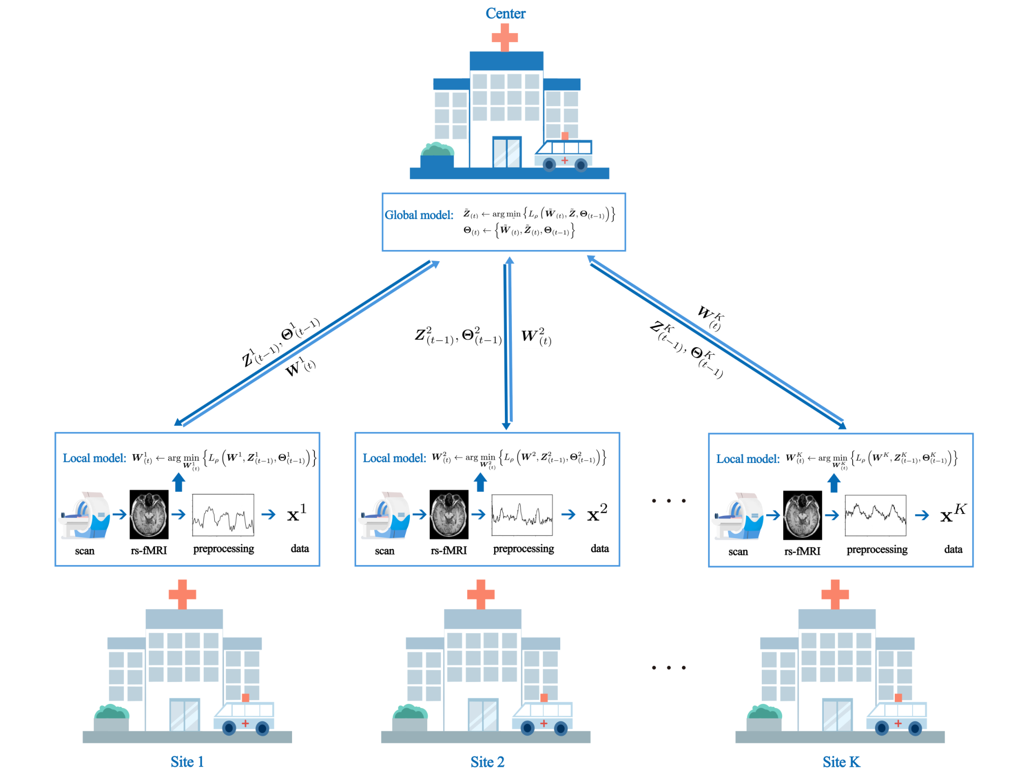
To address the above issues, we propose a federated joint estimator for the simultaneous learning of multiple BNs with continuous optimization. In pursuit of computational efficiency, we convert the traditional combinatorial BN structure learning problem into a continuous numerical optimization problem inspired by the NOTEARS method (Zheng et al. 2018). To capture the heterogeneity, we learn multiple BNs from multi-site data but with similar structures by introducing the group fused lasso penalty instead of learning a single BN. To lighten the data-sharing barriers, we study the structure learning of multiple BNs in the federated learning (FL) setting, which is a natural method to tackle the data-sharing problem (Pfitzner et al. 2021). We refer to the proposed NOTEARS-based Personalized Federated Learning framework of learning multiple BNs’ structures as NOTEARS-PFL, whose whole protocol is shown in Figure 1.

Refer to caption — Figure 1: Illustration of the learning framework of NOTEARS-PFL. Each site stores and processes rs-fMRI data locally. In the $t$ -th iteration, each site estimates the local weighted adjacency matrix $\bm{W}^{k}_{(t)}$ through the local update step. Then, each site transmits the estimated local matrix to the center. Center updates the global weighted adjacency matrices $\tilde{\bm{Z}}_{(t)}$ through the global update step based on the received $\tilde{\bm{W}}_{(t)}=\{\bm{W}^{1}_{(t)},\ldots,\bm{W}^{K}_{(t)}\}$ . Finally, the center transmits the estimated global matrix to each site for the $(t+1)$ -th iteration update.

The merits of the proposed NOTEARS-PFL are multi-fold.

•

NOTEARS-PFL is capable of learning site-specific BNs from multi-site rs-fMRI data, which makes full use of the multi-site data while still being flexible enough to capture the site-specific BN structures.
•

NOTEARS-PFL is subtly fitted in an FL framework without sharing and exchanging the original data.
•

NOTEARS-PFL overcomes the computational intractability of traditional BNs by transforming the discrete combinatorial optimization to continuous numerical optimization.
•

NOTEARS-PFL can effectively detect the common abnormal FC in MDD patients among multiple sites, especially the connectivity between the insula, thalamus cortex, and middle temporal gyrus. Meanwhile, NOTEARS-PFL can also identify the site-specific abnormal FC due to the differences in scanners, protocols, and patient populations.

The paper is organized as follows. In Section 2, we briefly review directed FC estimation methods for rs-fMRI data and BN structure learning with continuous optimization. We present the formulation and optimization approach of NOTEARS-PFL in Section 3. We conduct simulation experiments to validate NOTEARS-PFL in Section 4, and analyze the real-world multi-site rs-fMRI data in Section 5. Finally, we conclude this paper in Section 6.

2 Related Work

2.1 Directed FC Estimation Methods for rs-fMRI Data

The directed FC, also known as effective FC, helps depict the abnormalities or dysfunction of the brain connectivity network (Smith 2012) and shows how information flows in the brain connectivity network (Henry and Gates 2017). Based on rs-fMRI data, many directed FC estimation methods have been developed, including the following four types.

(1) Granger causality (GC). GC establishes a model in the framework of vector autoregression (VAR) and determines the edges to be added after considering the autoregressive effect of each region (Granger 1969; Liao et al. 2009). GC is applied to detect the effects of psychostimulants on youths with attention deficit hyperactivity disorder (ADHD) (Peterson et al. 2009). However, when GC is applied to analyze specific individuals, heterogeneity across individuals may lead to spurious results (Molenaar 2004).

(2) Dynamic Causal Modeling (DCM). DCM is a method to capture nonlinear relationships between brain regions that may be affected by different stimuli during scanning (Friston et al. 2003), and has been used to detect the propagation of epileptic seizures (Murta et al. 2012). The limitation of DCM is that it cannot handle large amounts of ROIs or analysis group rs-fMRI data. (Friston et al. 2011).

(3) Constraint-based methods. Constraint-based methods estimate directed edges by conditional independence tests. Common constraint-based methods include Peter Spirtes, and Clark Glymour (PC) algorithm (Spirtes and Glymour 1991), conservative PC (CPC) (Ramsey et al. 2006), fast causal inference (FCI) (Spirtes 2001), and cyclic causal discovery (CCD) (Richardson 1996). The PC algorithm can obtain reliable networks on data aggregated across individuals (Smith et al. 2011). However, according to results from Smith et al. 2011, PC can detect the existence of edges but can not accurately determine the directions at the individual level.

(4) Score-based methods. Score-based methods define a score function that measures how well the BN structure fits the observed data and searches for the best network structure. Standard score-based methods include greedy equivalent search (GES) (Chickering 2002), independent multiple-sample greedy equivalent search (IMaGES) (Ramsey et al. 2010), and group iterative multiple model Estimation (GIMME) (Gates and Molenaar 2012). Score-based methods typically require large samples to identify edges and directions, which limits the utility of these methods when using rs-fMRI data for individual-level analysis (Mumford and Ramsey 2014). Meanwhile, the performance of score-based methods is poor on data with a large number of ROIs, which makes it difficult to analyze the complete parcellation of the brain. Due to the combinatorial acyclicity constraint of DAG, it is often hard to find BN with the optimal score. And its scalability is also limited (Liu et al. 2022).

2.2 BN Structure Learning with Continuous Optimization

In this work, we focus on BN learning. BN is a probabilistic graphical model that captures dependencies among a collection of random variables. Each model is associated with a directed network $\mathcal{G}=(V,E)$ , where the vertex set $V$ corresponds to the random variables and the edge set $E$ corresponds to the set of conditional independence (Drton and Maathuis 2017).

BN models the conditional independence among random variables via Markov properties (Cowell 1998; Marrelec et al. 2004). Denote $\bm{X}=(X_{1},\ldots,X_{d})^{\top}$ that satisfies the local Markov property with respect to a DAG $\mathcal{G}$ if

X_{v}\bot X_{\mbox{\scriptsize nd}_{\mathcal{G}}(v)\backslash\mbox{\scriptsize pa}_{\mathcal{G}}(v)}\mid X_{\mbox{\scriptsize pa}_{\mathcal{G}}(v)},

where ${\rm pa}_{\mathcal{G}}(v)=\{w\in V:\{w,v\}\in E\}$ denotes the parents of node $v$ in $\mathcal{G}$ , ${\rm nd}_{\mathcal{G}}(v)=V\backslash\mbox{de}_{\mathcal{G}}(v)$ denotes the non-descendants of $v$ in $\mathcal{G}$ with $\mbox{de}_{\mathcal{G}}(v)=\{w\in V:w=v\;\mbox{or}\;v\rightarrow\ldots\rightarrow w\;\mbox{in}\;G\}$ representing the descendants of $v$ in $\mathcal{G}$ .

Alternatively, if $\bm{X}$ is a continuous random vector and it has a density $\mathbb{P}(\bm{X})$ with respect to a product measure, then the local Markov property is equivalent to the following factorization property (Verma and Pearl 1990),

\mathbb{P}(\bm{X})=\prod_{v=1}^{d}\mathbb{P}\left(X_{v}\mid X_{\mbox{\scriptsize pa}_{\mathcal{G}}(v)}\right).

(1)

The structure learning of BN is to estimate the DAG $\mathcal{G}$ using the observations from the density $\mathbb{P}(\bm{X})$ . Score-based methods seek the optimal $\mathcal{G}$ by minimizing the score function $\mathcal{S}(W)$ with respect to the corresponding weighted adjacency matrix $\bm{W}\in\mathbb{R}^{d\times d}$ , subject to that the induced graph $g(\bm{W})$ is a DAG; see the LHS of equation (2). The DAG constraint initiates a combinatorial optimization problem, which is computationally costly when $d$ is large.

Recently, Zheng et al. 2018 proposed a NOTEARS method which enforces the acyclicity via setting a smooth function $h(\bm{W})$ exactly at zero; see the RHS of equation (2). By this novel characterization of acyclicity, the resulting optimization problem can be solved efficiently using standard algorithms.

\begin{array}[]{cl}\min_{\bm{W}\in\mathbb{R}^{d\times d}}\mathcal{S}(\bm{W}),&\min_{\bm{W}\in\mathbb{R}^{d\times d}}\mathcal{S}(\bm{W}),\\ \text{ s.t. }g(\bm{W})\in\mathrm{DAGs},&\text{ s.t. }h(\bm{W})=0.\end{array}

(2)

Currently, NOTEARS has been extended to handle problems in many situations. For example, DAG Graph Neural Network (DAG-GNN) extends NOTEARS to solve nonlinear cases by incorporating neural networks (Yu et al. 2019). Graph AutoEncoder (GAE) extends NOTEARS and DAG-GNN into a graph autoencoder model, facilitating vector-valued variables (Ng et al. 2019). Pamfil et al. 2020 proposed DYNOTEARS method to learn dynamic BNs from time-series data. Huang et al. 2020 used reinforcement learning to find the optimal DAGs from incomplete data based on NOTEARS.

To the best of our knowledge, few studies have focused on using NOTEARS to learn personalized BNs from fMRI data. Zhang et al. 2022 proposed a joint BN estimation model to detect abnormal directed FC in schizophrenia (SZ) patients. However, the joint estimation model proposed by Zhang et al. 2022 is not applicable for the FL setting. Ng and Zhang 2022 proposed NOTEARS-ADMM model to estimate the structure of BN in FL setting. However, they did not consider the data heterogeneity, which can lead to model bias (Zhao et al. 2018; Jiang et al. 2022). Compared with Zhang et al. 2022 and Ng and Zhang 2022, the proposed NOTEARS-PFL is powerful because it captures the data heterogeneity, overcomes the data sharing barriers, and attains computational efficiency, simultaneously.

3 NOTEARS-based Personalized Federated Learning Framework

3.1 Preliminary

The BN associated with a DAG $\mathcal{G}$ can also be thought of as a structural equation model (Bollen 1989)

X_{i}=f_{i}(W_{i}^{T}\bm{X})+Z_{i},i=1,2,\ldots,d,

(3)

where $\bm{W}=\left(W_{1},\ldots,W_{d}\right)\in\mathbb{R}^{d\times d}$ denotes the weighted adjacency matrix whose nonzero coefficients correspond to the directed edges in $\mathcal{G}$ , $f_{i}$ ’s are functions related to the conditional distributions of $X_{i}$ ’s, and $Z_{i}$ ’s are jointly independent random noises. Equation (3) is equivalent to the local Markov property and factorization property introduced in Section 2 (Drton and Maathuis 2017).

We consider the linear structural equation model

X_{i}=W_{i}^{T}\bm{X}+Z_{i},i=1,2,\ldots,d.

(4)

Actually, the multivariate Gaussian distribution can be modeled as equation (4) with $Z_{i}$ ’s being independent Gaussian noises.

Let the data matrix $\mathbf{x}\in\mathbb{R}^{n\times d}$ . Zheng et al. 2018 formulates the structure learning of BNs as

	$\displaystyle\min_{\bm{W}\in\mathbb{R}^{d\times d}}$	$\displaystyle\frac{1}{2n}\left\\|\mathbf{x}-\mathbf{x}\bm{W}\right\\|_{F}^{2}+\lambda\\|\bm{W}\\|_{1},$		(5)
	$\displaystyle\mbox{s.t.}$	$\displaystyle h(\bm{W})=0,$		(5)

where

h(\bm{W}):=\operatorname{tr}\left(e^{\bm{W}\odot\bm{W}}\right)-d=0,

(6)

$\odot$ denotes the Hadamard product, $e^{A}=\sum_{k=0}^{\infty}\frac{1}{k!}A^{k}$ denotes the the matrix exponential operator (Leonard 1996), $\|A\|_{F}$ denotes the Frobenius norm, $\|A\|_{1}$ refers to the entry-wise $\ell_{1}$ norm and the tuning parameter $\lambda>0$ controls the amount of sparsity.

3.2 Problem Formulation

We now proceed to formulate our NOTEARS-PFL method, which can efficiently learn multiple heterogeneous BNs without sharing data.

We consider the setting in which there is a fixed set of $K$ sites in total, and each site has its own local dataset. The $k$ -th site holds $n_{k}$ i.i.d. samples, denoted by $\mathbf{x}^{k}=\left\{x^{k}_{i}\right\}_{i=1}^{n_{k}}\in\mathbb{R}^{{n_{k}}\times d}$ . Let $\mathcal{D}=\{\mathbf{x}^{1},\dots,\mathbf{x}^{K}\}$ be the $K$ overall observational datasets. The goal is to infer the $K$ weighted adjacency matrices $\tilde{\bm{W}}_{0}=\{\bm{W}^{1}_{0},\ldots,\bm{W}^{K}_{0}\}$ (correspond to the BN structures) using $\mathcal{D}$ .

To incorporate the heterogeneity among $K$ sites, we consider the following optimization problem:

	$\displaystyle\min_{\tilde{\bm{W}}}$	$\displaystyle\sum_{k=1}^{K}\frac{1}{2n_{k}}\left\\|\mathbf{x}^{k}-\mathbf{x}^{k}\bm{W}^{k}\right\\|_{F}^{2}+\mathcal{R}(\bm{\tilde{W}}),$		(7)
	$\displaystyle\quad\quad\quad\mbox{s.t.}$	$\displaystyle h({\bm{W}}^{k})=0,\ k=1,\dots,K,$		(7)

where $h({\bm{W}}^{k})$ is defined in the same way as equation (6) and $\mathcal{R}(\tilde{\bm{W}})$ is a penalty function for inducing the similarity and sparsity within $\tilde{\bm{W}}$ .

With the data sharing constraint, we formulate equation (7) into the framework of ADMM, which is a natural solution to distributed learning and FL (Ng and Zhang 2022). Define a set of consensus variables $\tilde{\bm{Z}}=\{{\bm{Z}^{1},\ldots,\bm{Z}^{K}}\}$ , which can be thought of as the global weighted adjacency matrices, in contrast to the local weighted adjacency matrices $\tilde{\bm{W}}$ . Then we rewrite equation (7) as

$\displaystyle\min_{\tilde{\bm{W}},\tilde{\bm{Z}}}$	$\displaystyle\sum_{k=1}^{K}\mathcal{L}(\bm{W}^{k},\mathbf{x}^{k})+\mathcal{R}(\tilde{\bm{Z}}),$	(8)
$\displaystyle\mbox{s.t. }$	$\displaystyle h(\bm{Z}^{k})=0,$
	$\displaystyle\bm{W}^{k}=\bm{Z}^{k},\quad k=1,\ldots,K,$

where

\mathcal{L}(\bm{W}^{k},\mathbf{x}^{k}):=\frac{1}{2n_{k}}\left\|\mathbf{x}^{k}-\mathbf{x}^{k}\bm{W}^{k}\right\|_{F}^{2},

(9)

$h({\bm{Z}}^{k})$ is defined in the same way as equation (6), and $\mathcal{R}(\tilde{\bm{Z}})$ is defined by

\mathcal{R}(\tilde{\bm{Z}}):=\lambda_{1}\sum_{k=1}^{K}\|\bm{Z}^{k}\|_{1}+\lambda_{2}\sum_{k=1}^{K-1}\|\bm{Z}^{k+1}-\bm{Z}^{k}\|_{F},

(10)

where $\lambda_{1}>0$ controls the sparsity of $\bm{Z}^{k}$ and $\lambda_{2}>0$ controls the similarity within $\tilde{\bm{Z}}$ .

The general optimization procedure can be summarized as follows. First, each site estimates the local weighted adjacency matrix $\bm{W}^{k}$ by using local dataset $\mathbf{x}^{k}$ . Then, instead of transmitting the original data, each site only transmits its local weighted adjacency matrix to the center. After that, the center updates the global weighted adjacency matrices $\tilde{\bm{Z}}_{0}=\{{\bm{Z}^{1}_{0},\ldots,\bm{Z}^{K}_{0}}\}$ , based on received $\tilde{\bm{W}}_{0}$ , Finally, the center transmits the updated $\tilde{\bm{Z}}$ to each site, which performs the next update locally based $\bm{W}^{k}=\bm{Z}^{k}$ .

In the next subsection, we provide the computational details of NOTEARS-PFL.

3.3 Optimization Algorithm

By applying the augmented Lagrangian method (Bertsekas 2014), the equation (8) can be written as

	$\displaystyle L\left(\tilde{\bm{W}},\tilde{\bm{Z}},\bm{\Theta}\right)=$	$\displaystyle\sum_{k=1}^{K}\mathcal{L}(\bm{W}^{k},\mathbf{x}^{k})+\mathcal{R}(\tilde{\bm{Z}})+\sum_{k=1}^{K}\alpha_{k}h(\bm{Z}^{k})+\frac{\rho_{1}}{2}\sum_{k=1}^{K}\|h(\bm{Z}^{k})\|^{2}+\sum_{k=1}^{K}\operatorname{tr}(\beta_{k}(\bm{W}^{k}-\bm{Z}^{k})^{\top})$		(11)
		$\displaystyle+\frac{\rho_{2}}{2}\sum_{k=1}^{K}\left\\|\bm{W}^{k}-\bm{Z}^{k}\right\\|_{F}^{2},$		(11)

where $\tilde{\bm{\Theta}}=\{\rho_{1},\rho_{2},\alpha_{1},\ldots,\alpha_{K},\beta_{1},\ldots,\beta_{K}\}$ , $\rho_{1},\rho_{2}$ are the penalty coefficients, $\alpha_{1},\ldots,\alpha_{K}$ and $\beta_{1},\ldots,\beta_{K}$ are the Lagrange multiplies.

At the $t$ -th iteration, we can solve equation (11) as follows:

(1) Local update:

\tilde{\bm{W}}_{(t)}\leftarrow\arg\min_{\tilde{\bm{W}}}\left\{L\left(\tilde{\bm{W}},\tilde{\bm{Z}}_{(t-1)},\tilde{\bm{\Theta}}_{(t-1)}\right)\right\}.

(12)

(2) Global update:

\tilde{\bm{Z}}_{(t)}\leftarrow\arg\min_{\tilde{\bm{Z}}}\left\{L\left(\tilde{\bm{W}}_{(t)},\tilde{\bm{Z}},\tilde{\bm{\Theta}}_{(t-1)}\right)\right\}.

(13)

(3) Global update:

\tilde{\bm{\Theta}}_{(t)}\leftarrow\left\{\tilde{\bm{W}}_{(t)},\tilde{\bm{Z}}_{(t)},\tilde{\bm{\Theta}}_{(t-1)}\right\}.

(14)

3.3.1 Federated Local Update of $\tilde{\bm{W}}$

Taking the derivative of equation (11) with respect to $\tilde{\bm{W}}$ , we can update each $\bm{W}^{k}_{(t)}$ of $\tilde{\bm{W}}_{(t)}$ as

{\bm{W}^{k}_{(t)}}:=\underset{\bm{W}^{k}}{\arg\min}(\mathcal{L}(\bm{W}^{k},\mathbf{x}^{k})+\frac{\rho_{2,(t-1)}}{2}\left\|\bm{W}^{k}-\bm{Z}^{k}_{(t-1)}\right\|_{F}^{2}+\operatorname{tr}(\beta_{k,(t-1)}(\bm{W}^{k}-\bm{Z}^{k}_{(t-1)})^{\top})).

(15)

Let $U^{k}=\frac{1}{n_{k}}(\mathbf{x}^{k})^{\top}\mathbf{x}^{k}$ and assume $U^{k}+\rho_{2}I$ is invertible. Equation (15) has a closed form expression

\bm{W}^{k}_{(t)}=(U^{k}+\rho_{2,(t-1)}I)^{-1}(\rho_{2,(t-1)}\bm{Z}^{k}_{(t-1)}-\beta_{k,(t-1)}+U^{k}),

(16)

where the details of the derivation are given in Appendix A.

3.3.2 Federated Global Update of $\tilde{\bm{Z}}$

Similar to equation (15), we can update each $\bm{Z}^{k}_{(t)}$ of $\tilde{\bm{Z}}_{(t)}$ as

\bm{Z}^{k}_{(t)}:=\underset{\bm{Z}^{k}}{\arg\min}\{\mathcal{L}(\tilde{\bm{Z}})+\mathcal{R}(\tilde{\bm{Z}})\},

(17)

where

	$\displaystyle\mathcal{L}(\tilde{\bm{Z}}):=$	$\displaystyle\sum_{k=1}^{K}\alpha_{k,(t-1)}h(\bm{Z}^{k})+\frac{\rho_{1,(t-1)}}{2}\sum_{k=1}^{K}\|h(\bm{Z}^{k})\|^{2}+\frac{\rho_{2,(t-1)}}{2}\sum_{k=1}^{K}\left\\|\bm{W}^{k}_{(t)}-\bm{Z}^{k}\right\\|_{F}^{2})$
		$\displaystyle+\sum_{k=1}^{K}\operatorname{tr}(\beta_{k,(t-1)}(\bm{W}^{k}_{(t)}-\bm{Z}^{k})^{\top}).$

Algorithm 1 Dykstra-like iterative proximal algorithm (DIPA)

K

: Number of site;

\tilde{\bm{Z}}

: global adjacency matrices;

\tilde{\bm{W}}

: local adjacency matrices;

N

: The number of iterations;

\epsilon

: Tolerance.

\tilde{\bm{Z}}

: The result of equation (19).

\nabla\mathcal{L}_{k}\left(\bm{Z}^{k}\right)

= equation (20).

2: for

k=1,\ldots,K

\bm{U}^{k}=\bm{Z}^{k}-\frac{1}{C}\nabla\mathcal{L}\left(\bm{Z}^{k}\right)

4: end for

\bar{\bm{U}}\leftarrow

Transform (

\bm{U}^{k}

6: Set

\bm{A}_{0}=\bar{\bm{U}}

\bm{M}_{n}=0

\bm{Q}_{n}=0

7: for

n=0,\ldots,N

\bm{V}_{(n)}\leftarrow\operatorname{prox}_{\mathcal{R}2}\left(\bm{A}_{(n)}+\bm{M}_{(n)}\right)

, see equation (28).

\bm{M}_{(n+1)}\leftarrow\bm{A}_{(n)}+\bm{M}_{(n)}-\bm{V}_{(n)}

10:

\bm{A}_{(n+1)}\leftarrow\operatorname{prox}_{\mathcal{R}_{1}}\left(\bm{V}_{(n)}+\bm{Q}_{(n)}\right)

, see equation (25).

11:

\bm{Q}_{(n+1)}\leftarrow\bm{V}_{(n)}+\bm{Q}_{(n)}-\bm{A}_{(n+1)}

12: Break: if

\left\|\bm{A}_{(n+1)}-\bm{A}_{(n)}\right\|_{F}<\epsilon.

13: end for

14:

\bar{\bm{U}}\leftarrow

\bm{A}_{({N}+1)}

15:

\tilde{\bm{Z}}\leftarrow

Inverse-Transform (

\bar{\bm{U}}

16: return

\tilde{\bm{Z}}

Due to the acyclicity term $h(\bm{Z}^{k})$ , we are not able to derive a closed-form solution for equation (17). To tackle this issue, we utilize a proximal gradient method which constructs a quadratic approximation of $\mathcal{L}(\tilde{\bm{Z}})$ at $\tilde{\bm{Z}}_{(t-1)}$ , and updates $\tilde{\bm{Z}}_{(t)}$ by

\tilde{\bm{Z}}_{(t)}=\underset{\tilde{\bm{Z}}}{\arg\min}\{\mathcal{L}(\tilde{\bm{Z}}_{(t-1)})+\sum_{k=1}^{K}\left\langle\bm{Z}^{k}-\bm{Z}^{k}_{(t-1)},\nabla\mathcal{L}_{k}(\bm{Z}^{k}_{(t-1)})\right\rangle+\frac{C}{2}\sum_{k=1}^{K}\left\|\bm{Z}^{k}-\bm{Z}^{k}_{(t-1)}\right\|_{F}^{2}+\mathcal{R}(\tilde{\bm{Z}})\},

(18)

where $\nabla\mathcal{L}_{k}(\cdot)$ is the gradient of $\mathcal{L}_{k}(\cdot)$ , $C>0$ is the Lipschitz constant of $\nabla\mathcal{L}_{k}(\cdot)$ . After some simple manipulations of equation (18), e.g., ignoring constant terms of $\bm{Z}_{(t-1)}^{k}$ , we have

	$\displaystyle\tilde{\bm{Z}}_{(t)}$	$\displaystyle=\underset{\tilde{\bm{Z}}}{\arg\min}\{\frac{C}{2}\sum_{k=1}^{K}\left\\|\bm{Z}^{k}-\left(\bm{Z}_{(t-1)}^{k}-\frac{1}{L}\nabla\mathcal{L}_{k}\left(\bm{Z}_{t-1}^{k}\right)\right)\right\\|_{F}^{2}+\mathcal{R}(\tilde{\bm{Z}})\},$		(19)
		$\displaystyle=\operatorname{prox}_{C\mathcal{R}}\left(\sum_{k=1}^{K}\left(\bm{Z}_{(t-1)}^{k}-\frac{1}{L}\nabla\mathcal{L}_{k}\left(\bm{Z}_{(t-1)}^{k}\right)\right)\right),$		(19)

where

\nabla\mathcal{L}_{k}\left(\bm{Z}_{(t-1)}^{k}\right)=\alpha_{k,(t-1)}\nabla h(\bm{Z}^{k}_{(t-1)})+\rho_{1,(t-1)}h(\bm{Z}^{k}_{(t-1)})\nabla h(\bm{Z}^{k}_{(t-1)})-\beta_{k,(t-1)}+\rho_{2,(t-1)}(\bm{Z}^{k}_{(t-1)}-\bm{W}^{k}),

(20)

and $\operatorname{prox}_{g}(v)=\underset{x}{\arg\min}(\frac{1}{2}\|x-v\|_{F}^{2}+g(x))$ denotes the proximal operator.

Unlike the calculation of $\bm{W}^{k}$ , we cannot separate the equation (19) by $k$ because of the grouped constraint $\mathcal{R}(\tilde{\bm{Z}})$ . Instead, we must estimate the whole set of matrices $\tilde{\bm{Z}}_{(t)}$ jointly. Inspired by Gibberd and Nelson 2017, we use the following iterative proximal projection step to solve.

Let $\bm{U}^{k}=\bm{Z}_{(t-1)}^{k}-\frac{1}{C}\nabla\mathcal{L}_{k}\left(\bm{Z}_{(t-1)}^{k}\right)$ , and perform transform procedure (see AppendixB) for $\bm{U}^{k}\rightarrow\bar{\bm{U}}$ . Then, equation (19) can be re-written as

\underset{\bar{\bm{Z}}}{\min}\underbrace{\frac{1}{2}\left\|\bar{\bm{Z}}-\bar{\bm{U}}\right\|_{F}^{2}}_{\mathcal{L}(\bar{\bm{Z}})}+\underbrace{\lambda_{1}\|\bar{\bm{Z}}\|_{1}}_{\mathcal{R}_{1}(\bar{\bm{Z}})}+\underbrace{\lambda_{2}\|\bm{D}\bar{\bm{Z}}\|_{2,1}}_{\mathcal{R}_{2}(\bar{\bm{Z}})},

(21)

where $\bm{D}\in\mathbb{R}^{(K-1)\times K}$ is a backwards difference matrix of the form $D_{i,i}=-1,D_{i,i+1}=1\text{ for }i=1,\ldots,K-1$ , and $\|A\|_{2,1}\text{ := }\sum_{k}\left\|A_{k,\cdot}\right\|_{2}$ denotes the group $\ell_{2,1}$ norm. Actually, equation (21) is equivalent to the Group-Fused Lasso Signal Approximator (GFLSA) defined by Gibberd and Nelson 2017. We denote the objective in equation (21) by $f\left(\bar{\bm{U}};\lambda_{1},\lambda_{2}\right)=\operatorname{prox}_{\mathcal{R}_{1}+\mathcal{R}_{2}}\left(\bar{\bm{U}}\right)$ . Then, we adopt the Dykstra-like iterative proximal algorithm (DIPA) (Combettes and Pesquet 2011) to handle $\operatorname{prox}_{\mathcal{R}_{1}+\mathcal{R}_{2}}\left(\bar{\bm{U}}\right)$ and find a feasible solution for both the group fused lasso penalty and the lasso penalty. We summarize the details of iteration in Algorithm 1.

Algorithm 2 ADMM of NOTEARS-PFL

K

: Number of site;

\mathbf{x}^{k}

: Original data;

\tilde{\bm{Z}}_{(0)}

: Initial global adjacency matrices;

\rho_{1,0}

\rho_{2,0}

\alpha_{1,0},\ldots,\alpha_{K,0}

\beta_{1,0},\ldots,\beta_{K,0}

: Initial parameters;

T

: The maximum of iterations;

\epsilon

: Tolerance.

\hat{\bm{Z}^{k}}

: Estimated adjacency matrix.

for iterations

t=1

T

Local update step:

for site

k=1,\ldots,K

Update

\bm{W}^{k}_{(t)}

according to equation (16).

end for

Global update step:

for variables

\tilde{\bm{Z}}_{(t-1)}

\bm{\Theta}_{(t-1)}

in the center do

\bm{Z}^{k}_{(t)}\leftarrow

DIPA (

\bm{W}^{k}_{(t)},\bm{Z}^{k}_{(t-1)}

Update

\bm{{\tilde{\Theta}}}_{(t-1)}

according to equation (22).

end for

Break: if

\sum_{k=1}^{K}\frac{\left\|\bm{Z}^{k}_{(t)}-\bm{Z}^{k}_{(t-1)}\right\|_{F}}{\left\|\bm{Z}^{k}_{(t)}\right\|_{2}}<\epsilon.

end for

return

\tilde{\bm{Z}}=(\bm{Z}^{1}_{(T)},...,\bm{Z}^{K}_{(T)})

3.3.3 Federated Global Update of $\tilde{\bm{\Theta}}$

The update of $\tilde{\bm{\Theta}}$ follows the following iterative steps

$\displaystyle\beta_{k,t}$	$\displaystyle:=\beta_{k,t-1}+\rho_{2,t-1}\left(\bm{W}^{k}_{(t)}-\bm{Z}^{k}_{(t)}\right),$	(22)
$\displaystyle\alpha_{k,t}$	$\displaystyle:=\alpha_{k,t-1}+\rho_{1,t-1}h\left(\bm{Z}^{k}_{(t)}\right),$
$\displaystyle\rho_{1,t}$	$\displaystyle:=\gamma_{1}\rho_{1,t-1},$
$\displaystyle\rho_{2,t}$	$\displaystyle:=\gamma_{2}\rho_{2,t-1},$

where $\gamma_{1},\gamma_{1}\in\mathbb{R}$ are hyperparameters that respectively control the increasing speeds of the coefficients $\rho_{1},\rho_{2}$ . The overall ADMM algorithm of NOTEARS-PFL is thereby given in Algorithm 2.

4 Simulations

4.1 Simulation Design of Synthetic Data

We simulate synthetic data according to equation (4). First, we generate a random graph $G_{truth}$ based on Erdös–Rényi (ER) model (Erdös et al. 1960). To obtain a set of related graphs, we apply perturbations to $G_{truth}$ to create $K$ similar but different graphs $\tilde{G}=\{G^{1},\ldots,G^{K}\}$ . The details of the definition of perturbation are shown in Appendix C, and we denote the perturbation level as $p_{l}$ .

Given $\tilde{G}$ , we assign uniformly random edge weights to obtain $K$ weights matrices $\tilde{\bm{W}}=\{\bm{W}^{1},\ldots,\bm{W}^{K}\}$ , where the non-zero entries are sampled uniformly at random form $[-2,-0.5]\cup[0.5,2]$ . Given $\tilde{\bm{W}}$ , we generate the datasets $\mathcal{D}=\{\mathbf{x}^{1},\dots,\mathbf{x}^{K}\}$ based on equation (4) with standard Gaussian noise.

To evaluate and compare the performance of the proposed method, we apply the NOTEARS (Zheng et al. 2018) method to estimate each network independently from each site’s local data (NOTEARS-SIG for short), and apply the NOTEARS method to learn a common network structure for all contexts (NOTEARS-AVG for short), i.e., an “average” network that treats all site’s data as samples in one dataset. We also compare the performance between NOTEARS-ADMM (Ng and Zhang 2022) and the proposed method.

We use the following four metrics to evaluate the learning performance of different methods (see Appendix C for a detailed definition of metrics).

•

Edge arrowhead error:

$\text{\emph{Error}}=\frac{FP+FN}{TP+TN+FP+FN}.$ (23)
•

Edge arrowhead precision:

$\text{ \emph{Precision} }=\frac{TP}{TP+FP}.$

•

Edge arrowhead F-score:

\text{ \emph{F-score}}=2\cdot\frac{\text{ \emph{Precision} }\cdot\text{\emph{Recall} }}{\text{ \emph{Precision} }+\text{\emph{Recall}}},

where $\text{ \emph{Recall}}=TP/(TP+FN)$ .

•

Edge arrowhead structural Hamming distance (SHD): Given two structures, this measure is the minimum number of edges needed to convert the learned graph into the true one.

We compare the performance of the proposed NOTEARS-PFL, NOTEARS-SIG, NOTEARS-AVG, and NOTEARS-ADMM on the following three aspects.

Performance vs. the number of variable: We fix the number of sites $K=10$ , perturbation level $p_{l}=10\%$ , set the total sample size $n_{t}=\sum_{k=1}^{K}n_{k}$ equals to three times the number of variable $d$ ( $n_{t}=3d$ , $n_{k}=0.3d$ ), and compare the model performance of network structure learning for different variable number $d=10,20,30,40,50,60,70,80$ .

Performance vs. the number of site: We fix the number of variable $d=50$ , perturbation level $p_{l}=10\%$ . We set the total sample size $n_{t}=256$ , and distributed evenly across the number of site $K=2,4,8,16,32,64$ .

Performance vs. perturbation level: We fix the number of site $K=10$ , the number of variable $d=30$ , sample size $n_{t}=3d$ , and vary the perturbation level $p_{l}=5\%,10\%,15\%,20\%,30\%$ .

The evaluation metrics for one simulation run are averaged over the $K$ sites’ dataset, and we repeat each experiment $10$ times. The final evaluation metrics are thereby averaged over the ten simulation runs.

In the synthetic data experiment, we first evaluate the effect of the number of variables $d$ on the performance of each compared method. The results are shown in Figure 2. It is clear that NOTEARS-PFL performs the best among all the methods. The average arrowhead adjacency error of NOTEARS-PFL has a relatively low level ranging from $0.02$ to $0.13$ . In contrast, for NOTEARS-SIG, the average arrowhead adjacency error is far larger than NOTEARS-PFL, ranging from $0.04$ to $0.43$ . This may be because the sample size of a single dataset is too small for NOTEARS-SIG to give a satisfactory estimate. The same result is observed in the average arrowhead SHD. For the other two metrics, NOTEARS-PFL consistently results in higher average arrowhead precision and F-score than the other three methods. Compared with NOTEARS-SIG and NOTEARS-AVG, the average arrowhead precision of NOTEARS-PFL is also more stable with respect to different variable numbers, indicating that it can successfully identify most of the edges in high-dimensional settings.

We also test the effect of the number of sites $K$ on the performance of each method. The results are shown in Figure 3. Clearly, NOTEARS-PFL performs better than NOTEARS-SIG, NOTEARS-AVG, and NOTEARS-ADMM for all the tested cases. As $K$ increases, the performance of NOTEARS-SIG, NOTEARS-AVG decline rapidly. Although the performance of NOTEARS-PFL also decreases with the increase of $K$ , it still provides a relatively stable and satisfying performance. As expected, NOTEARS-SIG does not perform better at larger $K$ . A possible reason is that NOTEARS-SIG only utilizes the information of a single dataset whose sample size decreases with the increase of $K$ . On the contrary, NOTEARS-PFL works well in the setting with a large site number because information can be exchanged during optimization. These results are also consistent with the existing literature (Ng and Zhang 2022).

Finally, we examine the effect of the perturbation level $p_{l}$ on the performance of each method. The results are shown in Figure 4. It is clear that NOTEARS-PFL significantly outperforms the other three methods. It can be seen that with the increase of perturbation level, average arrowhead error and SHD increase significantly, while average arrowhead precision and F-score decrease. When the perturbation level is relatively low, the difference between the four methods is relatively small, but when the perturbation level is relatively large, the advantage of NOTEARS-PFL is more significant.

5 Application to Real-world rs-fMRI Data

5.1 Data and Preprocessing

(1) Data acquisition: The multi-site rs-fMRI datasets in this study were obtained from the DecNef Project Brain Data Repository¹¹ 1 https://bicr-resource.atr.jp/srpbsopen/, collected as part of the Japanese Strategic Research Program for the Promotion of Brain Science (SRPBS) database project (Tanaka et al. 2021). This dataset consists of 255 MDD patients (135 men versus 120 women) and 791 HC participants (426 men versus 365 women) from 8 sites. Some samples were discarded as some sites only have rs-fMRI data on HC participants. As a result, 238 MDD patients and 475 HC participants from 5 sites were used in this study (see Table 3). The demographic characteristics of all subjects in both datasets are summarized in Table 4.

(2) Data preprocessing : Each subject of the data underwent a single rs-fMRI session and a structural MRI session. During the fMRI scan, participants were asked to relax, stay awake and think about anything in particular. Detailed imaging parameters of rs-fMRI and T1-weighted (T1w) structural MRI at each site are shown in Table 5. We applied the following preprocessing steps to the data by using DPARSF (Yan and Zang 2010) software²² 2 http://www.rfmri.org/DPARSF. For each participant, we removed the first 10 MRI volumes. Slice-time correction and head motion were corrected on the remaining images. The T1-weighted images were unified segment segmentation and diffeomorphic anatomical registration. The rs-fMRI data were smoothed with a 6mm full-width at half-maximum Gaussian kernel and the Friston 24-parameter model was used to regress head motion effects further. Then, all the time series were filtered by linear detrending and a temporal band-pass filter (0.01 - 0.08 Hz).

(3) Feature extraction: After preprocessing, we estimated the time series of 116 ROIs based on the automated anatomical labeling (AAL) template (Tzourio-Mazoyer et al. 2002). Details of cortical and subcortical regions of interest (ROIs) defined in the AAL template are presented in Table 6 and Table 7. We selected 56 ROIs from 116 ROIs because these regions are considered to be related to MDD in the literature. The names of the selected ROIs are shown in bold in Table 6 and Table 7. The voxel-wise fMRI time courses were averaged into one regional average time course within each ROI. The data for each participant was then in the form of an $X\times$ 56 matrix ( $X$ sampling points in each regional average fMRI time course and 56 selected ROIs).

5.2 Experimental Setup

We randomly select 70% of MDD patients and HC participants from each site and aggregate their rs-fMRI data into the MDD discovery dataset and HC discovery dataset for that site, respectively. Similarly, we aggregate the remaining 30% into the MDD validation dataset and HC validation dataset for that site, respectively. We analyze the 5 sites’ discovery datasets of MDD patients, which are regarded as 5 related tasks. Then we can obtain a brain connection network of MDD for each site. To study the differences in brain FC, the brain connection networks of HC for five sites, which are viewed as another set of related tasks, are also obtained using the proposed NOTEARS-PFL method. According to the estimated BN structures, we analyze the abnormal FC in MDD by the following aspects.

5.2.1 Important Nodes Identification

By identifying important nodes, we reveal the aberrant nodal characteristics of the brain functional connectivity networks of MDD from multi-site datasets.

5.2.2 Overlapping Connections Identification

By identifying overlapping connections, we obtain the common functional connections for MDD patients from multiple sites. By comparing with the overlapping connections of HC participants, we further investigate the altered functional connections in MDD patients, which provide the potential biomarkers for clinic treatment of MDD.

5.2.3 Site-specific Connections Identification

By identifying the site-specific connections in different sites, we investigate the specific FC alterations in MDD at each site due to the differences in image acquisition protocols and patient populations at different sites.

5.2.4 Comparison with Other Methods

We randomly select 5 MDD patients and 5 HC participants from each site’s MDD validation dataset and HC validation dataset and repeat such selection 10 times. We then have 10 datasets containing MDD data and HC data from the 5 sites. Based on these datasets, we compare NOTEARS-PFL with NOTEARS-SIG and existing standard analysis methods of rs-fMRI data: GES (Chickering 2002), PC (Spirtes and Glymour 1991), and GC (Granger 1969). To further test whether NOTEARS-PFL is able to learn the differences between MDD patients and HC participants.

5.3 Experimental Results

In this section, we use NOTEARS-PFL method to analyze the multi-site rs-fMRI data from 5 sites. We can obtain the brain functional connection network of MDD patients for each site. To study the differences in brain FC, we also obtain the brain functional connection network of HC participants for each site.

5.3.1 Results of Important Nodes

To better understand the differences in brain FC between MDD patients and HC participants through the estimated directed brain networks from multi-site rs-fMRI data, we further use the connection degree to identify some important nodes. The connection degree (including in and out degree) is a commonly used measure of functional connectivity (Liu et al. 2022). More specifically, it represents the amount of directed functional connections. The greater the connection degree, the higher the effective FC. Identifying important nodes further helps to discover the nodes associated with the disease. Table 1 shows the differences in total connection degrees between MDD patients and HC participants at 5 sites. The total out connection degrees in Table 1 are 657 for MDD and 478 for HC, indicating that MDD has 37.4% effective FC than HC. Similarly, MDD also has 23.4% more effective FC than HC, with a total in connection degrees of 516 and 418, respectively. The rise of FC is an apparent robust biomarker of MDD disease (Zamoscik et al. 2014), which can also be found in our results.

Table 1: The top 10 out and in connection degrees of MDD patients and HC participants

	Index	ROI	Abbreviation	Degree		Index	ROI	Abbreviation	Degree
MDD (Out)	77	Thalamus	THA.L	75	HC (Out)	55	Fusiform gyrus	FFG.L	58
	29	Insula	INS.L	74		37	Hippocampus	HIP.L	57
	35	Cingulate gyurs, posterior part	PCG.L	72		31	Cingulate gyrus, anterior part	ACG.L	55
	33	Cingulate gyrus, mid part	DCG.L	68		38	Hippocampus	HIP.R	49
	34	Cingulate gyrus, mid part	DCG.R	67		9	Middle frontal gyrus, orbital	HIP.R	47
	31	Cingulate gyrus, anterior part	ACG.L	63		29	Insula	INS.L	46
	72	Caudate	CAU.R	62		77	Thalamus	THA.L	45
	71	Caudate	CAU.L	61		33	Cingulate gyrus, mid part	DCG.L	43
	55	Fusiform gyrus	FFG.L	58		56	Fusiform gyrus	FFG.R	40
	79	Heschl gyrus	HES.L	57		79	Heschl gyrus	HES.L	38
Total				657	Total				478
MDD (In)	24	Superior frontal gyrus, medial	SFGmed.R	79	HC (In)	3	Superior frontal gyrus, dorsolateral	SFGdor.L	55
	90	Inferior temporal gyrus	ITG.R	62		9	Middle frontal gyrus, orbital	ORBmid.L	48
	26	Superior frontal gyrus, medial orbital	ORBsupmed.R	59		26	Superior frontal gyrus, medial orbital	ORBsupmed.R	45
	89	Inferior temporal gyrus	ITG.L	54		90	Inferior temporal gyrus	ITG.R	44
	3	Superior frontal gyrus, dorsolateral	SFGdor.L	48		10	Middle frontal gyrus, orbital	ORBmid.R	41
	46	Cuneus	CUN.R	46		14	Inferior frontal gyrus, triangular	IFGtriang.R	40
	11	Inferior frontal gyrus, opercular	IFGoperc.L	45		24	Superior frontal gyrus, medial	SFGmed.R	39
	25	Superior frontal gyrus, medial orbital	ORBsupmed.L	42		1	Precentral gyrus	PreCG.L	38
	41	Amygdala	AMYG.L	41		89	Inferior temporal gyrus	ITG.L	36
	32	Cingulate gyrus, anterior part	ACG.R	40		6	Superior frontal gyrus, orbital	ORBsup.R	32
Total				516	Total				418

From Table 1, we can find some ROI nodes with high connection degrees, such as THA.L (thalamus), INS.L (insula), SFGmed.R (superior frontal gyrus, medial) in MDD, and FFG.L (fusiform gyrus) and HIP.L (hippocampus) in HC. Specifically, THA.L and INS.L have more outgoing connections in MDD than in HC. It indicates that THA.L and INS.L of MDD have a higher essential impact on other ROI nodes than HC. The result from NOTEARS-PFL is in line with literature (Kang et al. 2018; Avery et al. 2014; Porta-Casteràs et al. 2021). According to Kang et al. 2018, emerging evidence indicates that the enhanced thalamus FC is an important feature of the underlying pathophysiology of MDD. This abnormal FC is related to the core clinical symptoms of MDD, such as anxiety, memory, and attention. Our result further implies that the impaired FC of the hippocampus is potentially an important biomarker of MDD. Compared to HC, the bilateral hippocampus in MDD lack FC. As the core region of the limbic system, the hippocampus plays an important role in regulating motivation and emotion. The mode of emotion regulation in MDD may be related to the decreased FC of the hippocampus (Cao et al. 2012). SFGmed.R (superior frontal gyrus, medial) and ITG.R (inferior temporal gyrus) have more incoming connections than outgoing connections, which indicates that SFGmed.R and ITG.R are mainly affected by other ROI nodes. These findings are also consistent with the physiological discoveries of MDD disease (Porta-Casteràs et al. 2021).

5.3.2 Results of Overlapping Connections

Figure 5 depicts the overlapping connections between the directed networks of 5 sites of MDD patients and HC participants. The overlapping connection refers to the connection shared by five sites. We can use it to study the universal connection between MDD and compare the differences between MDD and HC. From Figure 5, we can find some abnormal functional connections in MDD: INS.R (insula) $\rightarrow$ ORBmid.R (middle frontal gyrus, orbital), INS.R (insula) $\rightarrow$ INS.L (insula), INS.R (insula) $\rightarrow$ ACG.R (cingulate gyrus, anterior part), PCG.L (cingulate gyurs, posterior part) $\rightarrow$ PCG.R (cingulate gyurs, posterior part), THA.L (thalamus) $\rightarrow$ CAU.R (caudate), STG.R (superior temporal gyrus) $\rightarrow$ MTG.R (middle temporal gyrus). Three common functional connections are associated with the insula, which further demonstrates the important role of the insula in identifying abnormal functional connections in MDD. The insula has been shown to be a potential primary biomarker for the diagnosis of MDD (McGrath et al. 2013). In MDD patients, the insula show increased FC with other limbic or paralimbic structures, particularly with the ventromedial prefrontal cortex (vmPFC) and orbitofrontal cortex (OFC) (Avery et al. 2014; Drevets et al. 2008), which is also illustrated in our results.

In addition to the abnormal insula structure in MDD patients, we also observe the abnormalities of FC in posterior cingulate gyurs, thalamus, inferior temporal gyrus, and middle temporal gyrus, which are also consistent with findings in the works of literature (Khundakar and Thomas 2009; Zhao et al. 2014). These cortices belong to the default mode network (DMN) and are considered to contribute greatly to MDD (Gong and He 2015). The abnormalities of FC in DMN have been reported in many MDD studies (Vasudev et al. 2018), especially the frontal lobe and temporal lobe. These lobes are suggested to be closely associated to the cognitive and information-processing abilities of MDD patients (Brzezicka 2013).

5.3.3 Results of Site-specific Connections

In this study, we are also interested in the connections specific to a site. A site-specific connection is a connection that only exists on one site. By identifying the site-specific connections in different sites, we can better understand the specificity of FC in MDD patients due to the differences in image acquisition protocols and patient populations at different sites. The site-specific connections of 5 sites of MDD patients are visualized in Figure 6. In the results of site 1, we can find the increased functional connection from frontal to pariental and from frontal to temporal, especially the increased afferent connections to precuneus. The precuneus is considered one of the hubs of DMN, which is generally associated with the rumination of negative and sad thoughts in MDD (Cheng et al. 2018). It has been shown to play a key role in identifying MDD (Peng et al. 2015). A study of effective FC in MDD has shown a significant increase in forward connectivity from the middle and inferior temporal cortical areas to the precuneus (Öngür et al. 2003), which is consistent with our study (the connections IFGoperc.L $\rightarrow$ PCUN.R, IFGtriang.L $\rightarrow$ PCUN.L).

Similarly, in site 2, we find the enhanced FC within the frontal cortex, particularly the connections associated with the orbitofrontal cortex (the connections ORBsup.L $\rightarrow$ ORBsupmed.L, MFG.L $\rightarrow$ ORBmid.R, AMYG.L $\rightarrow$ ORBmid.L). The increased FC in the orbitofrontal cortex in MDD patients is associated with emotionally negative self-perception (Cheng et al. 2016). The orbitofrontal cortex is also a part of the brain’s affective network (AN), and the increased functional connections of the orbitofrontal cortex in MDD have been consistently reported (Townsend et al. 2010). The different effective FC patterns of the orbitofrontal cortex can also be used to reveal different pathophysiological mechanisms of different depression types or groups.

5.3.4 Comparison Results with Other Methods

To further test whether NOTEARS-PFL is able to learn the differences between MDD patients and HC participants, we use different methods to learn the BN structures from the test validation dataset established in Section 5. Based on the learned BN structures, we perform a two-sample proportion test for each published overlapping connection of MDD in Figure 5, and report the $p$ -values in Table 2. The smaller $p$ value indicates that NOTEARS-PFL recognizes the connection more easily in MDD group than in HC group. We also included test results for NOTEARS-SIG, GES, PC, and GS for comparison. In order to ensure the consistency of measurement standards, we control these methods to learn the same sparsity network structure.

Table 2: Two-sample proportion tests for published overlapped connections.

Connection	NOTEARS-PFL	NOTEARS-SIG	GES	PC	GC
INS.R $\rightarrow$ INS.L	0.0002	0.0016	0.0022	0.0512	0.0057
INS.R $\rightarrow$ ORBmid.R	0.0012	0.0029	0.0055	0.0234	0.0133
THA.L $\rightarrow$ CAU.R	0.0016	0.0040	0.0126	0.1636	0.0264
PCG.L $\rightarrow$ PCG.R	0.0040	0.0091	0.0283	0.0984	0.0549
INS.R $\rightarrow$ ACG.R	0.0049	0.0234	0.0133	0.2625	0.0289
STG.R $\rightarrow$ MTG.R	0.0055	0.0264	0.0549	0.0721	0.0567
MTG.L $\rightarrow$ ORBmid.R	0.0126	0.0283	0.0264	0.1556	0.1018

6 Conclusion

In this work, we focus on learning the heterogeneous brain functional connectivity in MDD patients using multi-site data efficiently and with the data sharing constraint. To this end, we developed a toolbox called NOTEARS-PFL. To achieve the model heterogeneity and computational efficiency, NOTEARS-PFL is formulated as minimizing a group fused lasso penalized score function with a continuous constraint for DAG. Considering the data-sharing barriers, the objective is solved in a federated learning framework using the ADMM, where original data is not exchanged during the optimization process. The algorithm is fast because the local update step has a closed-form expression, and the global update step can be solved using an efficient iterative proximal projection method. Extensive experiments on synthetic data and real-world multi-site rs-fMRI datasets with MDD demonstrate the excellent performance of the proposed method. We highlight the usefulness of NOTERAS-PFL in analyzing multi-site rs-fMRI data and facilitating the study of MDD.

References

Avery et al. (2014) Jason A Avery, Wayne C Drevets, Scott E Moseman, Jerzy Bodurka, Joel C Barcalow, and W Kyle Simmons. Major depressive disorder is associated with abnormal interoceptive activity and functional connectivity in the insula. Biological Psychiatry, 76(3):258–266, 2014.
Belmaker and Agam (2008) Robert H Belmaker and Galila Agam. Major depressive disorder. New England Journal of Medicine, 358(1):55–68, 2008.
Bertsekas (2014) Dimitri P Bertsekas. Constrained optimization and Lagrange multiplier methods. Academic Press, 2014.
Bleakley and Vert (2011) Kevin Bleakley and Jean-Philippe Vert. The group fused lasso for multiple change-point detection. arXiv preprint arXiv:1106.4199, 2011.
Bollen (1989) Kenneth A Bollen. Structural equations with latent variables, volume 210. John Wiley & Sons, 1989.
Brzezicka (2013) Aneta Brzezicka. Integrative deficits in depression and in negative mood states as a result of fronto-parietal network dysfunctions. Acta Neurobiologiae Experimentalis (Wars), 73(3):313–325, 2013.
Cao et al. (2012) Xiaohua Cao, Zhifen Liu, Cheng Xu, Jianying Li, Qiang Gao, Ning Sun, Yong Xu, Yan Ren, Chunxia Yang, and Kerang Zhang. Disrupted resting-state functional connectivity of the hippocampus in medication-naive patients with major depressive disorder. Journal of Affective Disorders, 141(2-3):194–203, 2012.
Cassano and Fava (2002) Paolo Cassano and Maurizio Fava. Depression and public health: an overview. Journal of Psychosomatic Research, 53(4):849–857, 2002.
Cheng et al. (2016) Wei Cheng, Edmund T Rolls, Jiang Qiu, Wei Liu, Yanqing Tang, Chu-Chung Huang, XinFa Wang, Jie Zhang, Wei Lin, Lirong Zheng, et al. Medial reward and lateral non-reward orbitofrontal cortex circuits change in opposite directions in depression. Brain, 139(12):3296–3309, 2016.
Cheng et al. (2018) Wei Cheng, Edmund T Rolls, Jiang Qiu, Deyu Yang, Hongtao Ruan, Dongtao Wei, Libo Zhao, Jie Meng, Peng Xie, and Jianfeng Feng. Functional connectivity of the precuneus in unmedicated patients with depression. Biological Psychiatry: Cognitive Neuroscience and Neuroimaging, 3(12):1040–1049, 2018.
Chickering (2002) David Maxwell Chickering. Optimal structure identification with greedy search. Journal of Machine Learning Research, 3:507–554, 2002.
Combettes and Pesquet (2011) Patrick L Combettes and Jean-Christophe Pesquet. Proximal splitting methods in signal processing. In Fixed-point Algorithms for Inverse Problems in Science and Engineering, pages 185–212. Springer, 2011.
Cowell (1998) Robert Cowell. Introduction to inference for Bayesian networks. In Learning in Graphical Models, pages 9–26. Springer, 1998.
Drevets et al. (2008) Wayne C Drevets, Joseph L Price, and Maura L Furey. Brain structural and functional abnormalities in mood disorders: implications for neurocircuitry models of depression. Brain Structure and Function, 213(1):93–118, 2008.
Drton and Maathuis (2017) Mathias Drton and Marloes H Maathuis. Structure learning in graphical modeling. Annual Review of Statistics and Its Application, 4:365–393, 2017.
Erdös et al. (1960) Paul Erdös, Alfréd Rényi, et al. On the evolution of random graphs. Publ. Math. Inst. Hung. Acad. Sci, 5(1):17–60, 1960.
Friston et al. (2003) Karl J Friston, Lee Harrison, and Will Penny. Dynamic causal modelling. NeuroImage, 19(4):1273–1302, 2003.
Friston et al. (2011) Karl J Friston, Baojuan Li, Jean Daunizeau, and Klaas E Stephan. Network discovery with DCM. NeuroImage, 56(3):1202–1221, 2011.
Fu et al. (2008) Cynthia HY Fu, Janaina Mourao-Miranda, Sergi G Costafreda, Akash Khanna, Andre F Marquand, Steve CR Williams, and Michael J Brammer. Pattern classification of sad facial processing: toward the development of neurobiological markers in depression. Biological Psychiatry, 63(7):656–662, 2008.
Gates and Molenaar (2012) Kathleen M Gates and Peter CM Molenaar. Group search algorithm recovers effective connectivity maps for individuals in homogeneous and heterogeneous samples. NeuroImage, 63(1):310–319, 2012.
Gibberd and Nelson (2017) Alexander J Gibberd and James DB Nelson. Regularized estimation of piecewise constant gaussian graphical models: The group-fused graphical lasso. Journal of Computational and Graphical Statistics, 26(3):623–634, 2017.
Gong and He (2015) Qiyong Gong and Yong He. Depression, neuroimaging and connectomics: a selective overview. Biological Psychiatry, 77(3):223–235, 2015.
Granger (1969) Clive WJ Granger. Investigating causal relations by econometric models and cross-spectral methods. Econometrica: Journal of the Econometric Society, pages 424–438, 1969.
Hamilton et al. (2011) J Paul Hamilton, Gang Chen, Moriah E Thomason, Mirra E Schwartz, and Ian H Gotlib. Investigating neural primacy in major depressive disorder: multivariate Granger causality analysis of resting-state fMRI time-series data. Molecular Psychiatry, 16(7):763–772, 2011.
Henry and Gates (2017) Teague Henry and Kathleen Gates. Causal search procedures for fMRI: review and suggestions. Behaviormetrika, 44(1):193–225, 2017.
Huang et al. (2020) Xiaoshui Huang, Fujin Zhu, Lois Holloway, and Ali Haidar. Causal discovery from incomplete data using an encoder and reinforcement learning. arXiv preprint arXiv:2006.05554, 2020.
Ide et al. (2014) Jaime S Ide, Sheng Zhang, and R Li Chiang-shan. Bayesian network models in brain functional connectivity analysis. International Journal of Approximate Reasoning, 55(1):23–35, 2014.
Jia et al. (2015) Haomiao Jia, Matthew M Zack, William W Thompson, Alex E Crosby, and Irving I Gottesman. Impact of depression on quality-adjusted life expectancy (QALE) directly as well as indirectly through suicide. Social Psychiatry and Psychiatric Epidemiology, 50(6):939–949, 2015.
Jia et al. (2010) Zhiyun Jia, Xiaoqi Huang, Qizhu Wu, Tijiang Zhang, Su Lui, Junran Zhang, Nabin Amatya, Weihong Kuang, Raymond CK Chan, Graham J Kemp, et al. High-field magnetic resonance imaging of suicidality in patients with major depressive disorder. American Journal of Psychiatry, 167(11):1381–1390, 2010.
Jiang et al. (2022) Meirui Jiang, Zirui Wang, and Qi Dou. Harmofl: Harmonizing local and global drifts in federated learning on heterogeneous medical images. In Proceedings of the AAAI Conference on Artificial Intelligence, volume 36, pages 1087–1095, 2022.
Jin et al. (2019) Hao Jin, Yan Luo, Peilong Li, and Jomol Mathew. A review of secure and privacy-preserving medical data sharing. IEEE Access, 7:61656–61669, 2019.
Kandilarova et al. (2018) Sevdalina Kandilarova, Drozdstoy Stoyanov, Stefan Kostianev, and Karsten Specht. Altered resting state effective connectivity of anterior insula in depression. Frontiers in Psychiatry, 9:83, 2018.
Kang et al. (2018) Lijun Kang, Aixia Zhang, Ning Sun, Penghong Liu, Chunxia Yang, Gaizhi Li, Zhifen Liu, Yanfang Wang, and Kerang Zhang. Functional connectivity between the thalamus and the primary somatosensory cortex in major depressive disorder: a resting-state fMRI study. BMC psychiatry, 18(1):1–8, 2018.
Khundakar and Thomas (2009) Ahmad A Khundakar and Alan J Thomas. Morphometric changes in early-and late-life major depressive disorder: evidence from postmortem studies. International Psychogeriatrics, 21(5):844–854, 2009.
Koller and Friedman (2009) Daphne Koller and Nir Friedman. Probabilistic graphical models: principles and techniques. MIT press, 2009.
Leonard (1996) IE Leonard. The matrix exponential. SIAM Review, 38(3):507–512, 1996.
Li et al. (2020) Xiaoxiao Li, Yufeng Gu, Nicha Dvornek, Lawrence H Staib, Pamela Ventola, and James S Duncan. Multi-site fMRI analysis using privacy-preserving federated learning and domain adaptation: ABIDE results. Medical Image Analysis, 65:101765, 2020.
Liao et al. (2009) Wei Liao, Daniele Marinazzo, Zhengyong Pan, Qiyong Gong, and Huafu Chen. Kernel granger causality mapping effective connectivity on fMRI data. IEEE Transactions on Medical Imaging, 28(11):1825–1835, 2009.
Lin et al. (2016) Wuhong Lin, Huawang Wu, Yishu Liu, Dongsheng Lv, and Lihua Yang. A cca and ica-based mixture model for identifying major depression disorder. IEEE Transactions on Medical Imaging, 36(3):745–756, 2016.
Liu et al. (2013) Feng Liu, Wenbin Guo, Ling Liu, Zhiliang Long, Chaoqiong Ma, Zhimin Xue, Yifeng Wang, Jun Li, Maorong Hu, Jianwei Zhang, et al. Abnormal amplitude low-frequency oscillations in medication-naive, first-episode patients with major depressive disorder: a resting-state fMRI study. Journal of Affective Disorders, 146(3):401–406, 2013.
Liu et al. (2016) Mingxia Liu, Daoqiang Zhang, and Dinggang Shen. Relationship induced multi-template learning for diagnosis of Alzheimer’s disease and mild cognitive impairment. IEEE Transactions on Medical Imaging, 35(6):1463–1474, 2016.
Liu et al. (2017) Mingxia Liu, Jun Zhang, Pew-Thian Yap, and Dinggang Shen. View-aligned hypergraph learning for Alzheimer’s disease diagnosis with incomplete multi-modality data. Medical Image Analysis, 36:123–134, 2017.
Liu et al. (2022) Shuai Liu, Yixuan Qiu, Baojuan Li, Huaning Wang, and Xiangyu Chang. Learning multitask gaussian bayesian networks. arXiv preprint arXiv:2205.05343, 2022.
Marrelec et al. (2004) Guillaume Marrelec, Philippe Ciuciu, Mélanie Pélégrini-Issac, and Habib Benali. Estimation of the hemodynamic response in event-related functional MRI: Bayesian networks as a framework for efficient bayesian modeling and inference. IEEE Transactions on Medical Imaging, 23(8):959–967, 2004.
McGrath et al. (2013) Callie L McGrath, Mary E Kelley, Paul E Holtzheimer, Boadie W Dunlop, W Edward Craighead, Alexandre R Franco, R Cameron Craddock, and Helen S Mayberg. Toward a neuroimaging treatment selection biomarker for major depressive disorder. JAMA Psychiatry, 70(8):821–829, 2013.
Molenaar (2004) Peter CM Molenaar. A manifesto on psychology as idiographic science: Bringing the person back into scientific psychology, this time forever. Measurement, 2(4):201–218, 2004.
Mumford and Ramsey (2014) Jeanette A Mumford and Joseph D Ramsey. Bayesian networks for fMRI: a primer. NeuroImage, 86:573–582, 2014.
Murta et al. (2012) Teresa Murta, Alberto Leal, Marta I Garrido, and Patrícia Figueiredo. Dynamic causal modelling of epileptic seizure propagation pathways: a combined EEG–fMRI study. NeuroImage, 62(3):1634–1642, 2012.
Ng and Zhang (2022) Ignavier Ng and Kun Zhang. Towards federated bayesian network structure learning with continuous optimization. In International Conference on Artificial Intelligence and Statistics, pages 8095–8111. PMLR, 2022.
Ng et al. (2019) Ignavier Ng, Shengyu Zhu, Zhitang Chen, and Zhuangyan Fang. A graph autoencoder approach to causal structure learning. arXiv preprint arXiv:1911.07420, 2019.
Öngür et al. (2003) Dost Öngür, Amon T Ferry, and Joseph L Price. Architectonic subdivision of the human orbital and medial prefrontal cortex. Journal of Comparative Neurology, 460(3):425–449, 2003.
Pamfil et al. (2020) Roxana Pamfil, Nisara Sriwattanaworachai, Shaan Desai, Philip Pilgerstorfer, Konstantinos Georgatzis, Paul Beaumont, and Bryon Aragam. Dynotears: Structure learning from time-series data. In International Conference on Artificial Intelligence and Statistics, pages 1595–1605. PMLR, 2020.
Peng et al. (2015) Daihui Peng, Elizabeth B Liddle, Sarina J Iwabuchi, Chen Zhang, Zhiguo Wu, Jun Liu, Kaida Jiang, Lin Xu, Peter F Liddle, Lena Palaniyappan, et al. Dissociated large-scale functional connectivity networks of the precuneus in medication-naive first-episode depression. Psychiatry Research: Neuroimaging, 232(3):250–256, 2015.
Peterson et al. (2009) Bradley S Peterson, Marc N Potenza, Zhishun Wang, Hongtu Zhu, Andrés Martin, Rachel Marsh, Kerstin J Plessen, and Shan Yu. An fMRI study of the effects of psychostimulants on default-mode processing during stroop task performance in youths with ADHD. American Journal of Psychiatry, 166(11):1286–1294, 2009.
Pfitzner et al. (2021) Bjarne Pfitzner, Nico Steckhan, and Bert Arnrich. Federated learning in a medical context: a systematic literature review. ACM Transactions on Internet Technology (TOIT), 21(2):1–31, 2021.
Porta-Casteràs et al. (2021) Daniel Porta-Casteràs, Marta Cano, Joan A Camprodon, Colleen Loo, Diego Palao, Carles Soriano-Mas, and Narcís Cardoner. A multimetric systematic review of fMRI findings in patients with MDD receiving ECT. Progress in Neuro-Psychopharmacology and Biological Psychiatry, 108:110178, 2021.
Price et al. (2017) Rebecca B Price, Kathleen Gates, Thomas E Kraynak, Michael E Thase, and Greg J Siegle. Data-driven subgroups in depression derived from directed functional connectivity paths at rest. Neuropsychopharmacology, 42(13):2623–2632, 2017.
Ramsey et al. (2006) Joseph Ramsey, Peter Spirtes, and Jiji Zhang. Adjacency-faithfulness and conservative causal inference. In Proceedings of the Twenty-Second Conference on Uncertainty in Artificial Intelligence, pages 401–408, 2006.
Ramsey et al. (2010) Joseph D Ramsey, Stephen José Hanson, Catherine Hanson, Yaroslav O Halchenko, Russell A Poldrack, and Clark Glymour. Six problems for causal inference from fMRI. NeuroImage, 49(2):1545–1558, 2010.
Richardson (1996) Thomas Richardson. A polynomial-time algorithm for deciding markov equivalence of directed cyclic graphical models. In Proceedings of the Twelfth International Conference on Uncertainty in Artificial Intelligence, pages 462–469, 1996.
Ryali et al. (2012) Srikanth Ryali, Tianwen Chen, Kaustubh Supekar, and Vinod Menon. Estimation of functional connectivity in fMRI data using stability selection-based sparse partial correlation with elastic net penalty. NeuroImage, 59(4):3852–3861, 2012.
Smith (2012) Stephen M Smith. The future of fMRI connectivity. NeuroImage, 62(2):1257–1266, 2012.
Smith et al. (2011) Stephen M Smith, Karla L Miller, Gholamreza Salimi-Khorshidi, Matthew Webster, Christian F Beckmann, Thomas E Nichols, Joseph D Ramsey, and Mark W Woolrich. Network modelling methods for fMRI. NeuroImage, 54(2):875–891, 2011.
Smith et al. (2013) Stephen M Smith, Diego Vidaurre, Christian F Beckmann, Matthew F Glasser, Mark Jenkinson, Karla L Miller, Thomas E Nichols, Emma C Robinson, Gholamreza Salimi-Khorshidi, Mark W Woolrich, et al. Functional connectomics from resting-state fMRI. Trends in Cognitive Sciences, 17(12):666–682, 2013.
Spirtes (2001) Peter Spirtes. An anytime algorithm for causal inference. In International Workshop on Artificial Intelligence and Statistics, pages 278–285. PMLR, 2001.
Spirtes and Glymour (1991) Peter Spirtes and Clark Glymour. An algorithm for fast recovery of sparse causal graphs. Social Science Computer Review, 9(1):62–72, 1991.
Tanaka et al. (2021) Saori C Tanaka, Ayumu Yamashita, Noriaki Yahata, Takashi Itahashi, Giuseppe Lisi, Takashi Yamada, Naho Ichikawa, Masahiro Takamura, Yujiro Yoshihara, Akira Kunimatsu, et al. A multi-site, multi-disorder resting-state magnetic resonance image database. Scientific Data, 8(1):1–15, 2021.
Tibshirani (1996) Robert Tibshirani. Regression shrinkage and selection via the lasso. Journal of the Royal Statistical Society: Series B (Methodological), 58(1):267–288, 1996.
Tong et al. (2022) Jiayi Tong, Chongliang Luo, Md Nazmul Islam, Natalie E Sheils, John Buresh, Mackenzie Edmondson, Peter A Merkel, Ebbing Lautenbach, Rui Duan, and Yong Chen. Distributed learning for heterogeneous clinical data with application to integrating COVID-19 data across 230 sites. NPJ Digital Medicine, 5(1):1–8, 2022.
Townsend et al. (2010) Jennifer D Townsend, Nicole K Eberhart, Susan Y Bookheimer, Naomi I Eisenberger, Lara C Foland-Ross, Ian A Cook, Catherine A Sugar, and Lori L Altshuler. fMRI activation in the amygdala and the orbitofrontal cortex in unmedicated subjects with major depressive disorder. Psychiatry Research: Neuroimaging, 183(3):209–217, 2010.
Tzourio-Mazoyer et al. (2002) Nathalie Tzourio-Mazoyer, Brigitte Landeau, Dimitri Papathanassiou, Fabrice Crivello, Octave Etard, Nicolas Delcroix, Bernard Mazoyer, and Marc Joliot. Automated anatomical labeling of activations in SPM using a macroscopic anatomical parcellation of the MNI MRI single-subject brain. NeuroImage, 15(1):273–289, 2002.
Vasudev et al. (2018) Akshya Vasudev, Michael J Firbank, Joseph S Gati, Emily Ionson, and Alan J Thomas. BOLD activation of the ventromedial prefrontal cortex in patients with late life depression and comparison participants. International Psychogeriatrics, 30(5):629–634, 2018.
Verma and Pearl (1990) Thomas Verma and Judea Pearl. Causal networks: Semantics and expressiveness. In Machine Intelligence and Pattern Recognition, volume 9, pages 69–76. Elsevier, 1990.
Vos et al. (2017) Theo Vos, Amanuel Alemu Abajobir, Kalkidan Hassen Abate, Cristiana Abbafati, Kaja M Abbas, Foad Abd-Allah, Rizwan Suliankatchi Abdulkader, Abdishakur M Abdulle, Teshome Abuka Abebo, Semaw Ferede Abera, et al. Global, regional, and national incidence, prevalence, and years lived with disability for 328 diseases and injuries for 195 countries, 1990–2016: a systematic analysis for the global burden of disease study 2016. The Lancet, 390(10100):1211–1259, 2017.
Wang et al. (2022) Nan Wang, Dongren Yao, Lizhuang Ma, and Mingxia Liu. Multi-site clustering and nested feature extraction for identifying autism spectrum disorder with resting-state fMRI. Medical Image Analysis, 75:102279, 2022.
Yan and Zang (2010) Chaogan Yan and Yufeng Zang. Dparsf: a MATLAB toolbox for" pipeline" data analysis of resting-state fMRI. Frontiers in Systems Neuroscience, page 13, 2010.
Ye et al. (2015) Ming Ye, Tianliang Yang, Peng Qing, Xu Lei, Jiang Qiu, and Guangyuan Liu. Changes of functional brain networks in major depressive disorder: a graph theoretical analysis of resting-state fMRI. PloS One, 10(9):1–16, 2015.
Yu et al. (2019) Yue Yu, Jie Chen, Tian Gao, and Mo Yu. Dag-gnn: Dag structure learning with graph neural networks. In International Conference on Machine Learning, pages 7154–7163. PMLR, 2019.
Zamoscik et al. (2014) Vera Zamoscik, Silke Huffziger, Ulrich Ebner-Priemer, Christine Kuehner, and Peter Kirsch. Increased involvement of the parahippocampal gyri in a sad mood predicts future depressive symptoms. Social Cognitive and Affective Neuroscience, 9(12):2034–2040, 2014.
Zhang et al. (2022) Gemeng Zhang, Biao Cai, Aiying Zhang, Zhuozhuo Tu, Li Xiao, Julia M Stephen, Tony W Wilson, Vince D Calhoun, and Yu-Ping Wang. Detecting abnormal connectivity in schizophrenia via a joint directed acyclic graph estimation model. NeuroImage, 260, 2022.
Zhao et al. (2014) Y-J Zhao, M-Y Du, X-Q Huang, S Lui, Z-Q Chen, J Liu, Y Luo, X-L Wang, GJ Kemp, and Q-Y Gong. Brain grey matter abnormalities in medication-free patients with major depressive disorder: a meta-analysis. Psychological Medicine, 44(14):2927–2937, 2014.
Zhao et al. (2018) Yue Zhao, Meng Li, Liangzhen Lai, Naveen Suda, Damon Civin, and Vikas Chandra. Federated learning with non-iid data. arXiv preprint arXiv:1806.00582, 2018.
Zheng et al. (2018) Xun Zheng, Bryon Aragam, Pradeep K Ravikumar, and Eric P Xing. Dags with no tears: Continuous optimization for structure learning. Advances in Neural Information Processing Systems, 31, 2018.

Supplementary Materials

Appendix A Derivation of Federated Local Update Step

To solve the subproblem as shown in equation (15), we first drop the subscript $t$ to lighten the notation, which leads to

\underset{\bm{W}^{k}}{\min}f(\bm{W}^{k}):=\mathcal{L}(\bm{W}^{k},\mathbf{x}^{k})+\operatorname{tr}(\beta_{k}(\bm{W}^{k}-\bm{Z}^{k})^{\top})+\frac{\rho_{2}}{2}\left\|\bm{W}^{k}-\bm{Z}^{k}\right\|_{F}^{2}.

(24)

Let $U^{k}=\frac{1}{n_{k}}(\mathbf{x}^{k})^{\top}\mathbf{x}^{k}$ . The first term of the equation (24) can be written as

	$\displaystyle\mathcal{L}(\bm{W}^{k},\mathbf{x}^{k})$	$\displaystyle=\frac{1}{2n_{k}}\left\\|\mathbf{x}^{k}-\mathbf{x}^{k}\bm{W}^{k}\right\\|_{F}^{2},$
		$\displaystyle=\frac{1}{2n_{k}}\operatorname{tr}((\mathbf{x}^{k}-\mathbf{x}^{k}\bm{W}^{k})^{\top}(\mathbf{x}^{k}-\mathbf{x}^{k}\bm{W}^{k})),$
		$\displaystyle=\frac{1}{2n_{k}}\operatorname{tr}((\mathbf{x}^{k})^{\top}\mathbf{x}^{k}-(\bm{W}^{k})^{\top}(\mathbf{x}^{k})^{\top}\mathbf{x}^{k}-(\mathbf{x}^{k})^{\top}\mathbf{x}^{k}\bm{W}^{k}+(\bm{W}^{k})^{\top}(\mathbf{x}^{k})^{\top}\mathbf{x}^{k}\bm{W}^{k}),$
		$\displaystyle=\frac{1}{2}\operatorname{tr}\left(U^{k}-(\bm{W}^{k})^{\top}U^{k}-U^{k}\bm{W}^{k}+(\bm{W}^{k})^{\top}U^{k}\bm{W}^{k}\right),$
		$\displaystyle=\frac{1}{2}\operatorname{tr}\left(U^{k}-2(\bm{W}^{k})^{\top}U^{k}+(\bm{W}^{k})^{\top}U^{k}\bm{W}^{k}\right).$

Similarly, the third term of equation (24) can be written as

	$\displaystyle\frac{\rho_{2}}{2}\\|\bm{W}^{k}-\bm{Z}^{k}\\|_{F}^{2}$	$\displaystyle=\frac{\rho_{2}}{2}\operatorname{tr}\left(\left(\bm{W}^{k}-\bm{Z}^{k}\right)^{\top}\left(\bm{W}^{k}-\bm{Z}^{k}\right)\right),$
		$\displaystyle=\frac{\rho_{2}}{2}\operatorname{tr}\left((\bm{W}^{k})^{\top}\bm{W}^{k}-2(\bm{W}^{k})^{\top}\bm{Z}^{k}+(\bm{Z}^{k})^{\top}\bm{Z}^{k}\right).$

Therefore, we have

	$\displaystyle f(\bm{W}^{k})$	$\displaystyle=\frac{1}{2}\operatorname{tr}(U^{k}-2(\bm{W}^{k})^{\top}U^{k}+(\bm{W}^{k})^{\top}U^{k}\bm{W}^{k})+\operatorname{tr}(\beta_{k}(\bm{W}^{k})^{\top}-\beta_{k}(\bm{Z}^{k})^{\top})+\frac{\rho_{2}}{2}\operatorname{tr}((\bm{W}^{k})^{\top}\bm{W}^{k}$
		$\displaystyle-2(\bm{W}^{k})^{\top}\bm{Z}^{k}+(\bm{Z}^{k})^{\top}\bm{Z}^{k}),$
		$\displaystyle=\frac{1}{2}\operatorname{tr}(-2(\bm{W}^{k})^{\top}U^{k}+(\bm{W}^{k})^{\top}U^{k}\bm{W}^{k})+\operatorname{tr}(\beta_{k}(\bm{W}^{k})^{\top})\frac{\rho_{2}}{2}\operatorname{tr}((\bm{W}^{k})^{\top}\bm{W}^{k}-2(\bm{W}^{k})^{\top}\bm{Z}^{k}+c,$

and its derivative is given by

	$\displaystyle\nabla_{\bm{W}^{k}}f\left(\bm{W}^{k}\right)$	$\displaystyle=\frac{1}{2}(-2U^{k}+((U^{k})^{\top}+U^{k})\bm{W}^{k})+\beta_{k}+\frac{\rho_{2}}{2}(2\bm{W}^{k}-2\bm{Z}^{k}),$
		$\displaystyle=-U^{k}+U^{k}\bm{W}^{k}+\beta_{k}+\rho_{2}\bm{W}^{k}-\rho_{2}\bm{Z}^{k},$
		$\displaystyle=(U^{k}+\rho_{2}I)\bm{W}^{k}-U^{k}+\beta_{k}-\rho_{2}\bm{Z}^{k}.$

Assuming $U^{k}+\rho_{2}I$ is invertible, solving $\nabla_{\bm{W}^{k}}f\left(\bm{W}^{k}\right)=0$ yields the solution

\bm{W}^{k}=(U^{k}+\rho_{2}I)^{-1}(\rho_{2}\bm{Z}^{k}-\beta_{k}+U^{k}).

Appendix B Details on the Federated Global Update Step

We provide details of the DIPA algorithm in the federated global update step. For convenience, we introduce the following procedures and discuss how to transform $K$ matrices into one matrix, so that we can re-write equation (19) into vector form.

Transform: Given $K$ matrices $\tilde{\bm{M}}=\{{M^{1},\ldots,M^{K}}\}$ . For each $k=1,\ldots,K$ , $M^{k}\in\mathbb{R}^{d\times d}$ . Transform $M^{k}$ into vector form, denote as $m^{k}=\left(M_{i,j}^{k}\mid\text{ for }i,j=1,\ldots,d\right)^{\top}$ . Then, construct a matrix $\bar{\bm{M}}=\left(m^{1},\ldots,m^{K}\right)^{\top}\in\mathbb{R}^{K\times d^{2}}$ .

Inverse-Transform: The inverse-transform reverses the steps of the transform, which to transform the matrix $\bar{\bm{M}}\in\mathbb{R}^{K\times d^{2}}$ to $K$ matrices $\tilde{\bm{M}}=\{{M^{1},\ldots,M^{K}}\}$ .

The core of DIPA algorithm is to compute the separate proximal operators for $\mathcal{R}_{1}$ and $\mathcal{R}_{2}$ . And then the iterative projection can be used to find a feasible point. The proximal operator for the $\ell_{1}$ term $\operatorname{prox}_{\mathcal{R}_{1}}\left(\bar{\bm{U}}\right)$ is given by the soft-thresholding operator [Tibshirani 1996].

	$\displaystyle\operatorname{prox}_{\mathcal{R}_{1}}\left(\bar{\bm{U}};\lambda_{1}\right)$	$\displaystyle=\underset{\bar{\bm{Z}}}{\arg\min}\frac{1}{2}\left\\|\bar{\bm{Z}}-\bar{\bm{U}}\right\\|_{F}^{2}+\lambda_{1}\\|\bar{\bm{Z}}\\|_{1},$		(25)
		$\displaystyle=\operatorname{sign}(\bar{\bm{U}})\odot\max\left(\|\bar{\bm{U}}\|-\lambda_{1},\mathbf{0}\right).$		(25)

where the max and sign functions act in an element-wise manner and $\odot$ denotes element-wise multiplication.

The calculation of group-fused lasso proximal operator $\operatorname{prox}_{\mathcal{R}_{2}}\left(\bar{\bm{U}}\right)$ is more complex, and there is no obvious closed-form solution. We tackle this through a block-coordinate descent approach [Bleakley and Vert 2011]. Then, the proximal operator for the group smoothing aspect of the regularizer can be written as:

\operatorname{prox}_{\mathcal{R}_{2}}\left(\bar{\bm{U}};\lambda_{2}\right)=\underset{\bar{\bm{Z}}}{\arg\min}\frac{1}{2}\left\|\bar{\bm{Z}}-\bar{\bm{U}}\right\|_{F}^{2}+\lambda_{2}\|\bm{D}\bar{\bm{Z}}\|_{2,1}.

(26)

Let $\bm{A}=\bm{D}\bar{\bm{Z}}$ and construct $\bar{\bm{Z}}$ as a sum of differences via $Z_{k,\bullet}=\bm{a}+\sum_{i=1}^{K-1}\bm{A}_{i,\bullet},\left(\text{ where }\bm{a}=Z_{1,\bullet}\right)$ . Then we can interpret the proximal operator as a group lasso probem [Bleakley and Vert 2011].

\bm{A}:=\underset{\bm{A}}{\arg\min}\frac{1}{2}\|\bar{\bm{U}}_{cen}-\bar{\bm{R}}_{cen}\bm{A}\|_{F}^{2}+\lambda_{2}\|\bm{A}\|_{2,1},

(27)

where $\bm{X}_{cen}$ denotes a column centered matrix and $\bm{R}\in\mathbb{R}^{K\times(K-1)}$ is a matrix with entries $R_{i,j}=1$ for $i>j$ and $0$ otherwise. The problem above can be solved through a block-coordinate descent strategy, sequentially updating the solution for each block $\bm{A}_{k,\bullet}$ for $k=1,\ldots,K-1$ . We can then construct a solution for $\bar{\bm{Z}}$ by summing the differences. And the optimal value for $\bm{a}$ is given by $\bm{a}=\mathbf{1}_{1,T}(\bm{U}-\bm{R}\bm{A})$ . Correspondingly, the proximal operator for $\mathcal{R}_{2}$ is

\operatorname{prox}_{\mathcal{R}_{2}}\left(\bar{\bm{U}};\lambda_{2}\right)=\left(\bm{a}^{\top},\left(\bm{a}+\bm{A}_{1,\bullet}\right)^{\top},\ldots,\left(\bm{a}+\sum_{i=1}^{K-1}\bm{A}_{i,\bullet}\right)^{\top}\right)^{\top}.

(28)

Appendix C Details of the Synthetic Data Generating

We followed the similar synthetic data generate procedure as in [Liu et al. 2022]. The key is how to create similar but different graphs by applying perturbations.

Perturbation level: Denote the adjacency matrix of $G_{truth}$ as $A_{t}=(a^{t}_{ij})\in\mathbb{R}^{d\times d}$ , where $a^{t}_{ij}=1$ if there is an edge from node $i$ to node $j$ , and $a^{t}_{ij}=0$ otherwise, $i,j=1,\ldots,d$ . Then the generated BN, denoted by $G_{gen}$ , is constructed in the following way. Let $A_{g}$ be the adjacency matrix of $G_{gen}$ , and define the perturbation level as the ratio of the number of changed edges in $A_{g}$ to the number of all possible edges. For example, if the perturbation level is $10\%$ , we first set $A_{g}=A_{t}$ , and then randomly select $10\%$ of the off-diagonal elements $a^{t}_{ij}(i\neq j)$ in $A_{t}$ . For each selected element $a^{t}_{ij}$ , if $a^{t}_{ij}=0$ , then we set $a^{g}_{ij}=1$ (adding edge); if $a^{t}_{ij}=1$ , then with probability $1/2$ we set $a^{g}_{ij}=0$ (deleting edge), otherwise let $a^{g}_{ji}=1$ (reversing edge). We generate $K$ graphs $\tilde{G}=\{G^{1},\ldots,G^{K}\}$ by such a perturbation scheme.

Evaluation metric: Let $\{G_{output}^{1},\ldots,G_{output}^{K}\}$ represent the $K$ BN structures obtained from NOTEARS-PFL, NOTEARS-SIG, NOTEARS-AVG, NOTEARS-ADMM. The four basic statistics in the evaluation metrics are defined as follows: true positives (TP), the number of edges that are both in $G_{output}^{1}$ and $G^{1}$ ; false positives (FP), the number of edges that are present in $G_{output}^{1}$ but not in $G^{1}$ ; false negatives (FN), the number of edges that are present in $G^{1}$ but not in $G_{output}^{1}$ ; and true negatives (TN), the number of vertex pairs that are neither edges in $G^{1}$ nor in $G_{output}^{1}$ .

Appendix D Supplementary Tables

Table 3: Data summary of the datasets used in this study.

Center of Innovation in Hiroshima

(COI)

Kyoto University

(KUT)

University of Tokyo

(UTO)

Hiroshima Kajikawa Hospital

(HKH)

Hiroshima University Hospital

(HUH)

Total Subject

194

175

158

124

MDD Subject

HC Subject

124

159

MDD Percentage

36%

39%

53%

46%

rs-fMRI Frames

240

107

143

Table 4: Demographic characteristics of participants in multi-site datasets.

	Site	Number	Male/Female	Age	BDI
MDD	COI	70	31/39	45.0 ± 12.5	26.2 ± 9.9
	KUT	16	10 6	33.79±10.82	27.7 ± 10.1
	UTO	62	36/26	38.74 ±11.62	21.5±11.3
	HKH	33	20/13	44.8±11.5	28.5±8.7
	HUH	57	32/25	43.3±12.2	30.9±9.0
HC	COI	124	46/78	51.9 ± 13.4	8.2 ± 6.3
	KUT	159	93/66	36.51± 13.59	6.0 ± 5.4
	UTO	96	33/63	46.65±15.54	6.6 ± 6.5
	HKH	29	12 17	45.4±9.5	5.1±4.6
	HUH	67	30/37	45.6±9.4	5.6±4.3

Table 5: Imaging protocols for rs-fMRI and structural MRI in multi-site datasets.

COI

KUT

UTO

HKH

HUH

rs-fMRI

MRI scanner

Siemens

Verio

Siemens

TimTrio

MR750w

Siemens

Spectra

Sigma HDxt

Magnetic field strength

3.0T

Number of channels per coil

FoV (mm)

212

192

256

Matrix

64 x 64

Number of slices

Number of volumes

240

107

143

In-plane resolution (mm)

3.3 x 3.3

3.3125 X 3.3125

3.3 x 3.3

3.0 x 3.0

4.0 x 4.0

Slice thickness (mm)

3.2

Slice gap (mm)

0.8

TR (ms)

2500

2700

2000

TE (ms)

Flip angel (deg)

Slice acquisition order

Ascending

Total scan

time

10 min + 10s

(dummy)

10 min + 10s

(dummy)

10 min + 10s

(dummy)

4 min. 46s. + 14s

(dummy)

4 min. 46s. + 14s

(dummy)

Eye closed/fixate

Fixate

Structural MRI

FoV (mm)

256

225x 240

240

256

Matrix

256 x 256

240 x 256

256 x 256

Voxel size mm3

1 x 1x 1

0.9375 x 0.9375 x 1

1 x 1x 1.2

1 x 1x 1

TR (ms)

2300

2000

7.7

1900

6812

TE (ms)

2.98

3.4

3.1

2.38

1986

TI (ms)

900

990

400

900

450

Flip angel (deg)

Table 6: Description of ROIs in AAL template and their Montreal Neurological Institute (MNI) coordinates.

Index	Region name	Abbreviation	Lobe	x	y	z
1	Precentral gyrus	PreCG.L	Frontal	-38.65	-5.68	50.94
2	Precentral gyrus	PreCG.R	Frontal	41.37	-8.21	52.09
3	Superior frontal gyrus, dorsolateral	SFGdor.L	Frontal	-18.45	34.81	42.20
4	Superior frontal gyrus, dorsolateral	SFGdor.R	Frontal	21.90	31.12	43.82
5	Superior frontal gyrus, orbital	ORBsup.L	Frontal	-16.56	47.32	-13.31
6	Superior frontal gyrus, orbital	ORBsup.R	Frontal	18.49	48.10	-14.02
7	Middle frontal gyrus	MFG.L	Frontal	-33.43	32.73	35.46
8	Middle frontal gyrus	MFG.R	Frontal	37.59	33.06	34.04
9	Middle frontal gyrus, orbital	ORBmid.L	Frontal	-30.65	50.43	-9.62
10	Middle frontal gyrus, orbital	ORBmid.R	Frontal	33.18	52.59	-10.73
11	Inferior frontal gyrus, opercular	IFGoperc.L	Frontal	-48.43	12.73	19.02
12	Inferior frontal gyrus, opercular	IFGoperc.R	Frontal	50.20	14.98	21.41
13	Inferior frontal gyrus, triangular	IFGtriang.L	Frontal	-45.58	29.91	13.99
14	Inferior frontal gyrus, triangular	IFGtriang.R	Frontal	50.33	30.16	14.17
15	Inferior frontal gyrus, orbital	ORBinf.L	Frontal	-35.98	30.71	-12.11
16	Inferior frontal gyrus, orbital	ORBinf.R	Frontal	41.22	32.23	-11.91
17	Rolandic operculum	ROL.L	Frontal	-47.16	-8.48	13.95
18	Rolandic operculum	ROL.R	Frontal	52.65	-6.25	14.63
19	Supplementary motor area	SMA.L	Frontal	-5.32	4.85	61.38
20	Supplementary motor area	SMA.R	Frontal	8.62	0.17	61.85
21	Olfactory cortex	OLF.L	Frontal	-8.06	15.05	-11.46
22	Olfactory cortex	OLF.R	Frontal	10.43	15.91	-11.26
23	Superior frontal gyrus, medial	SFGmed.L	Frontal	-4.80	49.17	30.89
24	Superior frontal gyrus, medial	SFGmed.R	Frontal	9.10	50.84	30.22
25	Superior frontal gyrus, medial orbital	ORBsupmed.L	Frontal	-5.17	54.06	-7.40
26	Superior frontal gyrus, medial orbital	ORBsupmed.R	Frontal	8.16	51.67	-7.13
27	Gyrus rectus	REC.L	Frontal	-5.08	37.07	-18.14
28	Gyrus rectus	REC.R	Frontal	8.35	35.64	-18.04
29	Insula	INS.L	Insula and Cingulate Gyri	-35.13	6.65	3.44
30	Insula	INS.R	Insula and Cingulate Gyri	39.02	6.25	2.08
31	Cingulate gyrus, anterior part	ACG.L	Insula and Cingulate Gyri	-4.04	35.40	13.95
32	Cingulate gyrus, anterior part	ACG.R	Insula and Cingulate Gyri	8.46	37.01	15.84
33	Cingulate gyrus, mid part	DCG.L	Insula and Cingulate Gyri	-5.48	-14.92	41.57
34	Cingulate gyrus, mid part	DCG.R	Insula and Cingulate Gyri	8.02	-8.83	39.79
35	Cingulate gyurs, posterior part	PCG.L	Insula and Cingulate Gyri	-4.85	-42.92	24.67
36	Cingulate gyurs, posterior part	PCG.R	Insula and Cingulate Gyri	7.44	-41.81	21.87
37	Hippocampus	HIP.L	Temporal	-25.03	-20.74	-10.13
38	Hippocampus	HIP.R	Temporal	29.23	-19.78	-10.33
39	Parahippocampus	PHG.L	Temporal	-21.17	-15.95	-20.70
40	Parahippocampus	PHG.R	Temporal	25.38	-15.15	-20.47
41	Amygdala	AMYG.L	Temporal	-23.27	-0.67	-17.14
42	Amygdala	AMYG.R	Temporal	27.32	0.64	-17.50
43	Calcarine fissure and surrounding cortex	CAL.L	Occipital	-7.14	-78.67	6.44
44	Calcarine fissure and surrounding cortex	CAL.R	Occipital	15.99	-73.15	9.40
45	Cuneus	CUN.L	Occipital	-5.93	-80.13	27.22
46	Cuneus	CUN.R	Occipital	13.51	-79.36	28.23
47	Lingual gyrus	LING.L	Occipital	-14.62	-67.56	-4.63
48	Lingual gyrus	LING.R	Occipital	16.29	-66.93	-3.87
49	Superior occipital lobe	SOG.L	Occipital	-16.54	-84.26	28.17
50	Superior occipital lobe	SOG.R	Occipital	24.29	-80.85	30.59
51	Middle occipital lobe	MOG.L	Occipital	-32.39	-80.73	16.11
52	Middle occipital lobe	MOG.R	Occipital	37.39	-79.70	19.42
53	Inferior occipital lobe	IOG.L	Occipital	-36.36	-78.29	-7.84
54	Inferior occipital lobe	IOG.R	Occipital	38.16	-81.99	-7.61
55	Fusiform gyrus	FFG.L	Temporal	-31.16	-40.30	-20.23
56	Fusiform gyrus	FFG.R	Temporal	33.97	-39.10	-20.18
57	Postcentral gyrus	PoCG.L	Pariental	-42.46	-22.63	48.92
58	Postcentral gyrus	PoCG.R	Pariental	41.43	-25.49	52.55
59	Superior pariental gyrus	SPG.L	Pariental	-23.45	-59.56	58.96
60	Superior pariental gyrus	SPG.R	Pariental	26.11	-59.18	62.06
61	Inferior pariental gyrus	IPL.L	Pariental	-42.80	-45.82	46.74
62	Inferior pariental gyrus	IPL.R	Pariental	46.46	-46.29	49.54
63	Supramarginal gyrus	SMG.L	Pariental	-55.79	-33.64	30.45

Table 7: Continue table: Description of ROIs in AAL template and their Montreal Neurological Institute (MNI) coordinates.

Index	Region name	Abbreviation	Lobe	x	y	z
64	Supramarginal gyrus	SMG.R	Pariental	57.61	-31.50	34.48
65	Angular gyrus	ANG.L	Pariental	-44.14	-60.82	35.59
66	Angular gyrus	ANG.R	Pariental	45.51	-59.98	38.63
67	Precuneus	PCUN.L	Pariental	-7.24	-56.07	48.01
68	Precuneus	PCUN.R	Pariental	9.98	-56.05	43.77
69	Paracentral lobule	PCL.L	Frontal	-7.63	-25.36	70.07
70	Paracentral lobule	PCL.R	Frontal	7.48	-31.59	68.09
71	Caudate	CAU.L	Subcortial region	-11.46	11.00	9.24
72	Caudate	CAU.R	Subcortial region	14.84	12.07	9.42
73	Putamen	PUT.L	Subcortial region	-23.91	3.86	2.40
74	Putamen	PUT.R	Subcortial region	27.78	4.91	2.46
75	Pallidum	PAL.L	Subcortial region	-17.75	-0.03	0.21
76	Pallidum	PAL.R	Subcortial region	21.20	0.18	0.23
77	Thalamus	THA.L	Subcortial region	-10.85	-17.56	7.98
78	Thalamus	THA.R	Temporal	13.00	-17.55	8.09
79	Heschl gyrus	HES.L	Temporal	-41.99	-18.88	9.98
80	Heschl gyrus	HES.R	Temporal	45.86	-17.15	10.41
81	Superior temporal gyrus	STG.L	Temporal	-53.16	-20.68	7.13
82	Superior temporal gyrus	STG.R	Temporal	58.15	-21.78	6.80
83	Temporal pole: superior temporal gyrus	TPOsup.L	Temporal	-39.88	15.14	-20.18
84	Temporal pole: superior temporal gyrus	TPOsup.R	Temporal	48.25	14.75	-16.86
85	Middle temporal gyrus	MTG.L	Temporal	-55.52	-33.80	-2.20
86	Middle temporal gyrus	MTG.R	Temporal	57.47	-37.23	-1.47
87	Temporal pole: middle temporal gyrus	TPOmid.L	Temporal	-36.32	14.59	-34.08
88	Temporal pole: middle temporal gyrus	TPOmid.R	Temporal	44.22	14.55	-32.23
89	Inferior temporal gyrus	ITG.L	Temporal	-49.77	-28.05	-23.17
90	Inferior temporal gyrus	ITG.R	Temporal	53.69	-31.07	-22.32
91	Cerebellum crus 1	CRBLCrus1.L	Posterior Fossa	-36.07	-66.72	-28.93
92	Cerebellum crus 1	CRBLCrus1.R	Posterior Fossa	37.46	-67.14	-29.55
93	Cerebellum crus 2	CRBLCrus2.L	Posterior Fossa	-28.64	-73.26	-38.2
94	Cerebellum crus 2	CRBLCrus2.R	Posterior Fossa	32.06	-69.02	-39.95
95	Cerebellum 3	CRBL3.L	Posterior Fossa	-8.8	-37.22	-18.58
96	Cerebellum 3	CRBL3.R	Posterior Fossa	12.32	-34.47	-19.39
97	Cerebellum 4	CRBL45.L	Posterior Fossa	-15	-43.49	-16.93
98	Cerebellum 4	CRBL45.R	Posterior Fossa	17.2	-42.86	-18.15
99	Cerebellum 6	CRBL6.L	Posterior Fossa	-23.24	-59.1	-22.13
100	Cerebellum 6	CRBL6.R	Posterior Fossa	24.69	-58.32	-23.65
101	Cerebellum 7	CRBL7b.L	Posterior Fossa	-32.36	-59.82	-45.45
102	Cerebellum 7	CRBL7b.R	Posterior Fossa	33.14	-63.18	-48.46
103	Cerebellum 8	CRBL8.L	Posterior Fossa	-25.75	-54.52	-47.68
104	Cerebellum 8	CRBL8.R	Posterior Fossa	25.06	-56.34	-49.47
105	Cerebellum 9	CRBL9.L	Posterior Fossa	-10.95	-48.95	-45.9
106	Cerebellum 9	CRBL9.R	Posterior Fossa	9.46	-49.5	-46.33
107	Cerebellum 10	CRBL10.L	Posterior Fossa	-22.61	-33.8	-41.76
108	Cerebellum 10	CRBL10.R	Posterior Fossa	25.99	-33.84	-41.35
109	Vermis12	Vermis12	Posterior Fossa	0.76	-38.79	-20.05
110	Vermis3	Vermis3	Posterior Fossa	1.38	-39.93	-11.4
111	Vermis45	Vermis45	Posterior Fossa	1.22	-52.36	-6.11
112	Vermis6	Vermis6	Posterior Fossa	1.14	-67.06	-15.12
113	Vermis7	Vermis7	Posterior Fossa	1.15	-71.93	-25.14
114	Vermis8	Vermis8	Posterior Fossa	1.15	-64.43	-34.08
115	Vermis9	Vermis9	Posterior Fossa	0.86	-54.87	-34.9
116	Vermis10	Vermis10	Posterior Fossa	0.36	-45.8	-31.68

Table 8: The overlapping connections between the directed networks of 5 sites of MDD patients and HC participants.

		From			To
	Index	ROI	Lobe	Index	ROI	Lobe
MDD	10	ORBmid.R	Frontal	6	ORBsup.R	Frontal
	24	SFGmed.R	Frontal	33	DCG.L	Insula and Cingulate Gyri
	30	INS.R	Insula and Cingulate Gyri	10	ORBmid.R	Frontal
	30	INS.R	Insula and Cingulate Gyri	29	INS.L	Insula and Cingulate Gyri
	30	INS.R	Insula and Cingulate Gyri	32	ACG.R	Insula and Cingulate Gyri
	33	DCG.L	Insula and Cingulate Gyri	3	SFGdor.L	Frontal
	35	PCG.L	Insula and Cingulate Gyri	36	PCG.R	Insula and Cingulate Gyri
	46	CUN.R	Occipital	45	CUN.L	Occipital
	56	FFG.R	Temporal	11	IFGoperc.L	Frontal
	68	PCUN.R	Pariental	46	CUN.R	Occipital
	68	PCUN.R	Pariental	26	ORBsupmed.R	Frontal
	71	CAU.L	Subcortial region	6	ORBsup.R	Frontal
	77	THA.L	Subcortial region	72	CAU.R	Subcortial region
	82	STG.R	Temporal	86	MTG.R	Temporal
	85	MTG.L	Temporal	10	ORBmid.R	Frontal
	89	ITG.L	Temporal	1	PreCG.L	Frontal
HC	1	PreCG.L	Frontal	26	ORBsupmed.R	Frontal
	8	MFG.R	Frontal	9	ORBmid.L	Frontal
	23	SFGmed.L	Frontal	24	SFGmed.R	Frontal
	31	ACG.L	Insula and Cingulate Gyri	23	SFGmed.L	Frontal
	34	DCG.R	Insula and Cingulate Gyri	67	PCUN.L	Pariental
	38	HIP.R	Temporal	39	PHG.L	Temporal
	40	PHG.R	Temporal	3	SFGdor.L	Frontal
	82	STG.R	Temporal	8	MFG.R	Frontal
	86	MTG.R	Temporal	89	ITG.L	Temporal

Table 9: The site-specific connections between the directed networks of 5 sites of MDD patients.

		From			To
	Index	ROI	Lobe	Index	ROI	Lobe
Site 1	1	PreCG.L	Frontal	10	ORBmid.R	Frontal
	1	PreCG.L	Frontal	67	PCUN.L	Pariental
	2	PreCG.R	Frontal	67	PCUN.L	Pariental
	5	ORBsup.L	Frontal	39	PHG.L	Temporal
	6	ORBsup.R	Frontal	78	THA.R	Temporal
	7	MFG.L	Frontal	71	CAU.L	Subcortial region
	8	MFG.R	Frontal	82	STG.R	Temporal
	11	IFGoperc.L	Frontal	68	PCUN.R	Pariental
	13	IFGtriang.L	Frontal	67	PCUN.L	Pariental
	16	ORBinf.R	Frontal	56	FFG.R	Temporal
	24	SFGmed.R	Frontal	72	CAU.R	Subcortial region
	26	ORBsupmed.R	Frontal	42	AMYG.R	Temporal
	29	INS.L	Insula and Cingulate Gyri	8	MFG.R	Frontal
	42	AMYG.R	Temporal	87	TPOmid.L	Temporal
	55	FFG.L	Temporal	68	PCUN.R	Pariental
	77	THA.L	Subcortial region	31	ACG.L	Insula and Cingulate Gyri
	90	ITG.R	Temporal	56	FFG.R	Temporal
Site2	3	SFGdor.L	Frontal	7	MFG.L	Frontal
	4	SFGdor.R	Frontal	1	PreCG.L	Frontal
	5	ORBsup.L	Frontal	25	ORBsupmed.L	Frontal
	7	MFG.L	Frontal	10	ORBmid.R	Frontal
	15	ORBinf.L	Frontal	11	IFGoperc.L	Frontal
	24	SFGmed.R	Frontal	3	SFGdor.L	Frontal
	29	INS.L	Insula and Cingulate Gyri	9	ORBmid.L	Frontal
	29	INS.L	Insula and Cingulate Gyri	16	ORBinf.R	Frontal
	31	ACG.L	Insula and Cingulate Gyri	5	ORBsup.L	Frontal
	77	THA.L	Subcortial region	13	IFGtriang.L	Frontal
	81	STG.L	Temporal	24	SFGmed.R	Frontal
	85	MTG.L	Temporal	14	IFGtriang.R	Frontal
	33	DCG.L	Insula and Cingulate Gyri	35	PCG.L	Insula and Cingulate Gyri
	37	HIP.L	Temporal	12	IFGoperc.R	Frontal
	89	ITG.L	Temporal	42	AMYG.R	Temporal
	56	FFG.R	Temporal	35	PCG.L	Insula and Cingulate Gyri
	86	MTG.R	Temporal	5	ORBsup.L	Frontal
Site3	1	PreCG.L	Frontal	14	IFGtriang.R	Frontal
	2	PreCG.R	Frontal	57	PoCG.L	Pariental
	5	ORBsup.L	Frontal	26	ORBsupmed.R	Frontal
	7	MFG.L	Frontal	35	PCG.L	Insula and Cingulate Gyri
	11	IFGoperc.L	Frontal	23	SFGmed.L	Frontal
	13	IFGtriang.L	Frontal	46	CUN.R	Occipital
	23	SFGmed.L	Frontal	9	ORBmid.L	Frontal
	29	INS.L	Insula and Cingulate Gyri	3	SFGdor.L	Frontal
	33	DCG.L	Insula and Cingulate Gyri	42	AMYG.R	Temporal
	33	DCG.L	Insula and Cingulate Gyri	45	CUN.L	Occipital
	35	PCG.L	Insula and Cingulate Gyri	85	MTG.L	Temporal
	40	PHG.R	Temporal	11	IFGoperc.L	Frontal
	39	PHG.L	Temporal	6	ORBsup.R	Frontal
	72	CAU.R	Subcortial region	56	FFG.R	Temporal
	78	THA.R	Temporal	2	PreCG.R	Frontal
	80	HES.R	Temporal	82	STG.R	Temporal
Site4	2	PreCG.R	Frontal	24	SFGmed.R	Frontal
	5	ORBsup.L	Frontal	4	SFGdor.R	Frontal
	7	MFG.L	Frontal	29	INS.L	Insula and Cingulate Gyri
	9	ORBmid.L	Frontal	57	PoCG.L	Pariental
	12	IFGoperc.R	Frontal	14	IFGtriang.R	Frontal
	15	ORBinf.L	Frontal	7	MFG.L	Frontal
	24	SFGmed.R	Frontal	12	IFGoperc.R	Frontal
	30	INS.R	Insula and Cingulate Gyri	23	SFGmed.L	Frontal
	31	ACG.L	Insula and Cingulate Gyri	16	ORBinf.R	Frontal
	32	ACG.R	Insula and Cingulate Gyri	68	PCUN.R	Pariental
	34	DCG.R	Insula and Cingulate Gyri	5	ORBsup.L	Frontal
	37	HIP.L	Temporal	29	INS.L	Insula and Cingulate Gyri
	40	PHG.R	Temporal	16	ORBinf.R	Frontal
	41	AMYG.L	Temporal	3	SFGdor.L	Frontal
	45	CUN.L	Occipital	72	CAU.R	Subcortial region
	56	FFG.R	Temporal	7	MFG.L	Frontal
	68	PCUN.R	Pariental	15	ORBinf.L	Frontal
	87	TPOmid.L	Temporal	33	DCG.L	Insula and Cingulate Gyri
	90	ITG.R	Temporal	86	MTG.R	Temporal

Table 10: Continue table: The site-specific connections between the directed networks of 5 sites of MDD patients.

		From			To
	Index	ROI	Lobe	Index	ROI	Lobe
Site 5	1	PreCG.L	Frontal	24	SFGmed.R	Frontal
	2	PreCG.R	Frontal	46	CUN.R	Occipital
	7	MFG.L	Frontal	2	PreCG.R	Frontal
	10	ORBmid.R	Frontal	25	ORBsupmed.L	Frontal
	13	IFGtriang.L	Frontal	15	ORBinf.L	Frontal
	15	ORBinf.L	Frontal	4	SFGdor.R	Frontal
	24	SFGmed.R	Frontal	10	ORBmid.R	Frontal
	26	ORBsupmed.R	Frontal	77	THA.L	Subcortial region
	33	DCG.L	Insula and Cingulate Gyri	31	ACG.L	Insula and Cingulate Gyri
	34	DCG.R	Insula and Cingulate Gyri	38	HIP.R	Temporal
	36	PCG.R	Insula and Cingulate Gyri	39	PHG.L	Temporal
	39	PHG.L	Temporal	4	SFGdor.R	Frontal
	46	CUN.R	Occipital	77	THA.L	Subcortial region
	56	FFG.R	Temporal	32	ACG.R	Insula and Cingulate Gyri
	67	PCUN.L	Pariental	4	SFGdor.R	Frontal
	78	THA.R	Temporal	39	PHG.L	Temporal
	86	MTG.R	Temporal	16	ORBinf.R	Frontal
	89	ITG.L	Temporal	12	IFGoperc.R	Frontal

Learning Personalized Brain Functional Connectivity of MDD Patients from Multiple Sites via Federated Bayesian Networks

Abstract

1 Introduction

2 Related Work

2.1 Directed FC Estimation Methods for rs-fMRI Data

2.2 BN Structure Learning with Continuous Optimization

3 NOTEARS-based Personalized Federated Learning Framework

3.1 Preliminary

3.2 Problem Formulation

3.3 Optimization Algorithm

3.3.1 Federated Local Update of 𝑾~\tilde{\bm{W}}

3.3.2 Federated Global Update of 𝒁~\tilde{\bm{Z}}

3.3.3 Federated Global Update of 𝚯~\tilde{\bm{\Theta}}

4 Simulations

4.1 Simulation Design of Synthetic Data

5 Application to Real-world rs-fMRI Data

5.1 Data and Preprocessing

5.2 Experimental Setup

5.2.1 Important Nodes Identification

5.2.2 Overlapping Connections Identification

5.2.3 Site-specific Connections Identification

5.2.4 Comparison with Other Methods

5.3 Experimental Results

5.3.1 Results of Important Nodes

5.3.2 Results of Overlapping Connections

5.3.3 Results of Site-specific Connections

5.3.4 Comparison Results with Other Methods

6 Conclusion

References

Appendix A Derivation of Federated Local Update Step

Appendix B Details on the Federated Global Update Step

Appendix C Details of the Synthetic Data Generating

Appendix D Supplementary Tables

3.3.1 Federated Local Update of $\tilde{\bm{W}}$

3.3.2 Federated Global Update of $\tilde{\bm{Z}}$

3.3.3 Federated Global Update of $\tilde{\bm{\Theta}}$