Neural Network Adaptive Control with Long Short-Term Memory
Abstract
In this study, we propose a novel adaptive control architecture, which provides dramatically better transient response performance compared to conventional adaptive control methods. What makes this architecture unique is the synergistic employment of a traditional, Adaptive Neural Network (ANN) controller and a Long Short-Term Memory (LSTM) network. LSTM structures, unlike the standard feed-forward neural networks, can take advantage of the dependencies in an input sequence, which can contain critical information that can help predict uncertainty. Through a novel training method we introduced, the LSTM network learns to compensate for the deficiencies of the ANN controller during sudden changes in plant dynamics. This substantially improves the transient response of the system and allows the controller to quickly react to unexpected events. Through careful simulation studies, we demonstrate that this architecture can improve the estimation accuracy on a diverse set of uncertainties for an indefinite time span. We also provide an analysis of the contributions of the ANN controller and LSTM network to the control input, identifying their individual roles in compensating low and high-frequency error dynamics. This analysis provides insight into why and how the LSTM augmentation improves the system’s transient response. The stability of the overall system is also shown via a rigorous Lyapunov analysis.
I Introduction
Although Neural Networks (NN) is a fairly old concept [1], cheap and fast parallel computing unlocked their potential and lead to their current predominance in artificial intelligence and machine learning [2]. Computer vision and natural language processing are examples of fields that benefited greatly from these developments [3], [4]. Deep learning research produced derivatives of recurrent neural networks (RNN) such as long short-term memory (LSTM) [5] and gated recurrent unit [6], which are powerful structures for processing sequential data [7]. Reinforcement learning (RL) is another concept in machine learning that made advancements through applications of deep learning [8]. In RL, there exists a state that is updated with respect to an action selected by an agent that makes its choices based on observations to maximize its cumulative reward. A similarity can be drawn between control systems and RL where states, control inputs and feedback connections are parallel to states, actions, and observations, respectively. There are studies that take advantage of this fact to design RL-based controllers [9], [10].
The potential shown by earlier applications provides an incentive to utilize NN in adaptive control. The literature on this topic is extensive and well established [11, 12, 13, 14, 15]. Using an online-tuned feed-forward NN controller with adaptive update laws is proven to be stable and can successfully compensate the uncertainties [14]. However, if there are sudden changes in the uncertainty, the transient response can be oscillatory, which results in poor performance. This problem is addressed in [16] with the addition of external memory similar to a neural turing machine’s (NTM) [17]. However, unlike the common practice in NTMs, a feed-forward network, instead of an RNN, is used in [17]. Feed-forward networks that have access to only the current state cannot take full advantage of the dependencies in a sequence. Instead, using a recurrent structure with internal memory can increase the capability of sequence estimation and thus improve performance [18].
To address the above mentioned issues, we propose a novel control architecture that consists of an Adaptive Neural Network (ANN) controller and an LSTM. The purpose of the LSTM is to take advantage of the long and short-term dependencies in the input sequence to improve the transient response of the controller. Specifically, we train the LSTM in such a way that it learns to compensate for the inadequacies of the ANN controller in response to sudden and unexpected uncertainty variations. Offline training in closed-loop systems is challenging since the trained element affects the system dynamics. This closed loop structure similarly exists in RL applications and is addressed by previous studies [19, 20]. Inspired by these methods, we train the LSTM in a closed-loop setting to predict and compensate for the undesired transient error dynamics. We demonstrate via simulations that thanks to its predictive nature, LSTM offsets high-frequency errors, and thus complements the ANN controller, where the latter helps with handling the low-frequency dynamics.
To summarize, the contribution of this paper is a novel adaptive control framework that provides enhanced transient performance compared to conventional approaches. This is achieved by making the traditional ANN controller work in collaboration with an LSTM network that is trained in the closed-loop system.
II Problem Formulation
Consider the following plant dynamics
| (1a) | ||||
| (1b) | ||||
where is the accessible state vector, is the plant control input, is a known system matrix, is a state-dependent, possibly nonlinear, matched uncertainty, is a known control input matrix, and is a known output matrix, and is the plant output. Furthermore, it is assumed that the pair is controllable.
Assumption 1: The unknown matched uncertainty is continuous on a known compact set , where is a known positive constant.
Remark 1: The proposed method also applies for an unknown state matrix : Suppose that the plant dynamics are given by
| (2) |
where is an unknown state matrix and is a state-dependent, possibly nonlinear, matched uncertainty. The dynamics (2) can be written in the form of (1) and for a known matrix , by defining , given that the matching condition is satisfied for some feedback gain . This allows us to proceed assuming is known, without loss of generality.
To achieve command following of a bounded reference input , an error-integral state is defined as
| (3) |
which, when augmented with (1), yields the augmented dynamics
| (4a) | ||||
| (4b) | ||||
where is the augmented state, whose dimension is , and the system matrices , , and are
| (5a) | ||||
| (5b) | ||||
| (5c) | ||||
| (5d) | ||||
A baseline state feedback controller is designed as
| (6) |
where is selected such that is Hurwitz. Then, a reference model is defined as
| (7) |
where is the state vector of the reference model.
Although the matched uncertainty is of unknown structure, Assumption 1 implies that it can be approximated by a multi-layer neural network in the following form
| (8) |
such that
| (9) |
respectively, where the NN reconstruction error vector is unknown, but bounded by a known constant in the domain of interest . Such a bound depends on the number of hidden neurons and the weight matrices of the neural network and . The following assumption is necessary and is standard in the literature.
Assumption 2: The unknown ideal weights and are bounded by known positive constants such that and .
The input to the NN and the output of the hidden layer is given by
| (10a) | ||||
| (10b) | ||||
where the nonlinear activation function can be either sigmoid or tanh. Note that and are augmented with unity elements to account for hidden and outer layers biases, respectively. For the convenience of notation, we drop the overbar notation and write (8) as
| (11) |
where the dimensions of the weight matrices are loosely defined as and .
By defining the state tracking error as
| (12) |
the control objective is to make converge to zero while keeping all system signals bounded, with minimal transients. To achieve this, we use the control input
| (13) |
where is the baseline controller (6) that achieves the reference model dynamics (7) in the absence of uncertainty, is an adaptive neural network (ANN) controller designed to compensate for the matched uncertainty , and is the output of a long short-term memory (LSTM) network. Furthermore, is a robustifying term, which is defined subsequently.
In this paper, we focus our attention on enhancing the transient response of the closed-loop system. Particularly, we propose the synergistic employment of a traditional ANN controller and an LSTM network to obtain superior performance compared to conventional approaches. In what follows, we detail each control term in (13).
II-A Adaptive Neural Network Controller
The adaptive neural network (ANN) controller is designed to compensate for the matched nonlinear uncertainty , and is expressed as,
| (14) |
where represents an estimate of . Using (11), we define the estimate as
| (15) |
where is the input-to-hidden-layer weight matrix and is the hidden-to-output-layer weight matrix. These weights serve as estimates for the unknown ideal weights and , respectively. Through proper use of Taylor series-based arguments [14], the weights are updated using the adaptive laws
| (16a) | ||||
| (16b) | ||||
where and are symmetric positive definite matrices, serving as learning rates, is a scalar gain, and and are defined as
| (17) | ||||
Further, is the symmetric positive definite solution of the Lyapunov equation
| (18) |
for some symmetric positive definite matrix .
II-B Robustifying Term
The usage of the baseline controller, ANN controller, and the robustifying term is sufficient to solve the adaptive control problem, as demonstrated in [14] for nonlinear robot arm dynamics. However, for a generic multi-input multi-output (MIMO) dynamical system with matched uncertainties (1), a difficulty arises from the control input matrix . A subsidiary contribution of this paper is a modified robustifying term , which achieves the same stability results in [14], but for generic MIMO linear systems.
The robustifying term, (see (13)) is used to provide robustness against disturbances that arise from the high-order Taylor series terms [14]. For the considered MIMO linear plant dynamics, we propose a modified robustifying term which is defined as
| (19) |
with
| (20) |
where , and matrices and are defined in the previous subsection, whereas is given in (12). Furthermore, , where is a known upper bound for the absolute value of the sigmoid or tanh activation function derivatives, i.e. , where .
In order not to diverge from the main contribution of the paper, we defer the derivation of the ANN controller and the proposed modified robustifying term to the Appendix. The following section introduces the main focus of this paper.
III LSTM Network Design
We propose an LSTM network that works in coordination with the ANN controller to compensate for the uncertainties in the system, with better transients compared to conventional approaches. Combined usage of LSTM and ANN is not arbitrary. Indeed, in this section, we precisely define the separate roles of LSTM and ANN in the closed-loop system. The overall control architecture is given in Fig. 1. By taking the state tracking error as the input, the LSTM network computes the control input , which is fed to the plant to compensate for the ANN controller deficiencies. The motivation behind the LSTM network is to improve the transient response of the system and achieve faster convergence by taking advantage of the sequence prediction capabilities of the LSTM architecture.
Remark 2: LSTM network takes a sequence as an input and computes a sequence as the output. Hence, the sampling time of the network arises as a design parameter. The particular selection of the sampling time of the network is application dependent. A proper selection would match the sampling time at which the ANN is implemented, or it can be made larger to reduce the computational load. Nevertheless, the exact sampling time of the network is irrelevant in the proposed architecture since, as shown subsequently, the LSTM network can be trained offline to perform under a given sampling time.
Remark 3: The LSTM input sequence is generated from the continuous-time signal as
| (21) |
where is the sampling time of the LSTM. Furthermore, the output sequence of the LSTM is converted to the continuous-time signal which accounts for the control input of the LSTM, where
| (22) |

LSTM is a Recurrent Neural Network (RNN), which, unlike a conventional neural network structure, can learn the long-term dependencies of a sequence. This is accomplished with an additional hidden state, a cell state, and gates that update the states in a systematic way. One cell of LSTM can be seen in Fig. 2.
In Fig. 2, is the normalized version of the input sequence , is the hidden state, and is the cell state. , and are the recurrent weight matrices, input weight matrices, and bias vectors, respectively. denotes the gate activation function (sigmoid) and denotes the state activation function (). Subscripts , and denote forget gate, cell candidate, input gate, and output gate, respectively. , and denote the output of the gate operations. The superscript denotes the current time step and is the previous time step.
a) Forget Gate: The forget gate decides the relevant information that the cell state should take from the hidden state and the input. This is achieved with a sigmoid activation function.
| (23) |
b) Input Gate: The new information that is going to be added to the cell state is determined by the input gate and cell candidate. First, the hyperbolic tangent activation function is used to determine which information is going to be added to the cell state. Then, a sigmoid function is used to determine how much of this information is going to be added. This process is given as
| (24) |
| (25) |
c) Output Gate: The output gate decides how much of the cell state is going to be a part of the hidden state, using a sigmoid function as
| (26) |
The cell state is first erased using the forget gate , then new information is added through the input gate and cell candidate . This is achieved with the calculation
| (27) |
The gates mentioned above are used to determine the hidden state and the cell state for the next time step. The hidden state is updated using the output gate and cell state that is mapped between -1 and 1 using a function as
| (28) |
A fully connected layer is utilized to obtain an dimensional output to match the dimension of the control input as
| (29) |
where and are the weight matrix and bias vector of the fully connected layer, respectively. Then, the control input is constructed from the LSTM output as shown in (22).
The ability to learn the dependencies within sequences helps the LSTM to predict the evolution of an unknown function. It is noted that in a typical ANN implementation, the speed of the response can be increased by increasing the adaptation rates, which may cause undesired oscillations. With LSTM augmentation, faster convergence is achieved without the need for large learning rates. The training and implementation details of LSTM are explained in the following subsections.
III-A Training Method
Since the LSTM network operates in a closed loop system, the system states and the “truth”, which is the variable it is trying to estimate, are affected by the LSTM output (see Fig. 1). As the training progresses, the training data itself evolves with time, which allows the data to be used only once to train the network.
Our main philosophy to use LSTM is to compensate for the inadequacies of the conventional ANN controller: We know that ANN controllers are successful in compensating for the uncertainties asymptotically. However, adjusting their transient characteristics is not a trivial task. Instead of increasing the learning rates, LSTM provides better transients by actually predicting the type of transients and compensating accordingly. To achieve this, the goal for the LSTM is set to predict the estimation error of the ANN controller and compensate for this error. The estimation error of the ANN, or the deviation of the ANN controller input (14), , from the actual uncertainty, , is given as
| (30) |
The “truth” for the LSTM, or the desired signal for the LSTM to produce, is selected as
| (31) |
Therefore, LSTM provides a signal to the system that is an estimate of this truth, expressed as
| (32) |
During training, an uncertainty is introduced to the closed loop system, and LSTM is expected to learn , where is the control signal produced by ANN. Apart from , LSTM uses the state-tracking error , defined in (12), as its input (see Fig. 1). Every iteration of training affects the sequence that LSTM is trained on. This dynamic nature of training helps LSTM generalize to a set of functions that are not used in the training set. This is further emphasized in the Simulations Section.
Since there is no initial data set, the data needs to be collected by running the simulation with the initial LSTM weights. Since weight updates of the LSTM network also affect the system dynamics, new data needs to be collected after each episode of training. Before giving the LSTM output to the system, a gain “” scales . The role of this gain is to avoid an untrained LSTM network output from negatively affecting the system at the beginning of the training. starts from 0 and approaches 1 as the number of training iterations increases, then stays at 1 for the rest of the training. The training loop can be seen in Fig. 3.
III-B Normalization
The inputs of the LSTM network are the components of the tracking error vector , defined in (12). In order to make sure that these components are on a similar scale, normalization needs to be performed. However, since an initial training data set does not exist, data needs to be collected first in order to acquire the parameters for normalization. For collecting the normalization parameters only, the simulation is run with (see explanations after (32)), number of times. A gain is uniformly sampled from in every simulation run, to scale . This random scaling is used only during the normalization parameter collection, not during training.The LSTM network output is not injected to the system during this process. Within the collected data, the minimum, , and the maximum, , values, where ”” is used to refer the component, of each component of the error vector, are utilized to obtain the normalized input parameters as
| (33) |
III-C Stability Analysis
The following theorem displays the stability properties of the overall architecture.
Theorem 1: Consider the uncertain plant dynamics (1), subject to Assumptions 1 and 2, and the reference model (7). Let the control input be defined by (13), which consists of the baseline controller (6), the ANN controller defined by (14), (15) and (16), the robustifying term given in (19) and (20), and the LSTM controller explained in Section III. Then, given that (see Assumption 1), the solution is uniformly ultimately bounded (UUB) and converges to a predefined compact set, where and .
Proof:
The proof is deferred to the Appendix B. ∎
IV Simulations
In this section, the performance of the proposed control framework is examined using the short-period longitudinal flight dynamics. The short-period dynamics is given as [21]
| (34) |
where is the angle of attack (deg), is the pitch rate (deg/s), is the elevator deflection (deg), and is a state dependent matched uncertainty. Elevator magnitude and rate saturation limits are set as (deg) and (deg/s) [22]. The commanded input is the pitch rate. , , , , and are the stability and control derivatives.
The system matrices for a B-747 aircraft flying at the speed of 274 m/s at 6000 m altitude are given as [16]
| (35) |
The augmented state vector is
| (36) |
where is the angle of attack (rad), is the pitch rate (rad/s) and is the error-integral state (3). The input to the LSTM network is,
| (37) |
where , , and are the components of the normalized version of the state tracking error vector (33).
The baseline controller (6) is an LQR controller with cost matrices and . The nonlinear uncertainty, (see explanations after (32)) that the Long Short-Term Memory (LSTM) network (29) is trained on is defined as
| (38) |
The LSTM network is trained in the presence of an ANN controller (see Section II-A) that has a hidden layer consisting of four neurons. The learning rates in (16a) and (16b) are set as , and the Lyapunov matrix in (18) is set as . The outer weights and bias are initialized to zero. The inner weights and biases are initialized randomly between 0 and 1. In the simulations, the robustifying gain in (20) and scalar gain in (16a) and (16b) are set to 0.
The LSTM network contains one hidden layer with 128 neurons. The number of neurons in the input layer is 3 due to the number of state-tracking error components given as input to the network (37). Weights are initialized using Xavier Initialization [23]. The network is trained with stochastic gradient descent, and uses the Adam optimizer with a learning rate of 0.001, an L2 regularization factor of 0.0001, a gradient decay factor of 0.9, and a squared gradient decay factor of 0.999 [24]. The gradient clipping method is used with a threshold value of 1. The simulation step time is set to s. The minibatch size is taken as 1. To cover both low and high-valued uncertainties, is scaled by a parameter that took the alternating values of 0.2 and 2.
To obtain the normalization constants given in (33), the system is simulated 1000 times (), with the gain , (see Section III-B).
The loss function is chosen as Mean Squared Error (MSE) given as
| (39) |
where and are defined in (31) and (32),and is the number of data in the data set.
The proposed control framework is tested using the uncertainty defined as
| (40) |
where the function is chosen to have different types of sub-functions with different time intervals, compared to the training uncertainty (38).
IV-A Controller performance in the presence of small uncertainty
In this section, the effect of the proposed LSTM augmentation is examined using low-value uncertainties. For this purpose, is scaled by 0.1 during the tests. Then, the tracking performance, tracking error, and control inputs of the closed-loop system are compared with and without LSTM augmentation.


Figures 4 and 5 show the tracking and tracking error curves, respectively. While the error plots demonstrate that LSTM augmentation dramatically reduces both the error magnitudes and the transient oscillations, the error values are small enough to be ignored compared to the absolute values of the states. Therefore, one can conclude that in this scenario LSTM augmented and not-augmented cases show similar performances. In Fig. 6, the control inputs are presented. This figure shows that although LSTM augmentation does not affect the magnitude of the total control input in a meaningful manner, it provides damping to the oscillations by providing small but fast compensation to the introduced uncertainties. As we discussed above, since the ANN controller is already successful in compensating for the uncertainties, in this case, LSTM contribution is not prominent.
IV-B Controller performance in the presence of large uncertainty
In this section, the effect of the proposed LSTM augmentation is examined in the presence of high-valued uncertainties, which is obtained by using the as is.


Figures 7 and 8 demonstrate that LSTM augmentation substantially improves the transient response of the system, especially in pitch rate tracking, which is the output of interest (see (35)). It is noted that for this case, the same ANN controller and the LSTM network are used as in the small uncertainty case. Individual control inputs are shown in Fig. 9. In this case, unlike the low-uncertainty case, the LSTM augmentation makes the total control signal observably more agile, which is the main reason why excessive oscillations are prevented. This shows the LSTM network uses its memory to predict high-frequency changes in the system. It is noted that in this large uncertainty case the total control input is saturated. This is evident from Fig. 9, where the middle and the bottom sub-figures show the control signals created by the individual components of the overall controller, while the top sub-figure shows the total control input after saturation. The figure shows that the LSTM network produces large and very fast compensation, which causes saturation. Here, the rate saturation can be problematic since it creates some oscillations in the total control signal (see the zoomed section, blue line, in the top sub-figure). Although the oscillations could be acceptable since they are short-lived, we believe that this issue can also be tackled by training the LSTM network with saturation information. We explain this solution in the next section.
IV-C Addressing Saturation
To handle the saturation issue, we modified LSTM training by a) introducing the saturation limits to the plant dynamics during training, and b) informing the LSTM network whenever the control signal rate-saturates. The latter is achieved by providing additional input to the LSTM network as
| (41) |


The number of neurons in the input layer of the LSTM network is increased to 4 since the modified input to the LSTM network is
| (42) |
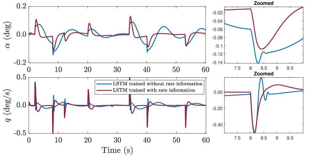
Figure 10 shows the LSTM network contribution and the total control inputs, with and without rate-limit information during training. It is seen that the LSTM network uses the rate-limit information to provide a smoother compensation. Figures 11 and 12 show the tracking and tracking error curves, respectively, when the LSTM network is trained using the rate-limit information. It is seen that the performance of the proposed controller remains similar for the case when LSTM is not trained using the saturation information, although the pitch rate shows initial small jumps at the instances of uncertainty switches.

V Summary
In this work, we propose a Long Short-Term Memory (LSTM) augmented adaptive neural network (ANN) control structure to improve the transient response of adaptive closed-loop control systems. We demonstrate that thanks to its time-series prediction capabilities, LSTM helps the ANN controller compensate for the uncertainties in a more agile fashion, resulting in dramatically improved tracking performance.
References
- [1] B. Macukow, “Neural networks–state of art, brief history, basic models and architecture,” in IFIP international conference on computer information systems and industrial management. Springer, 2016, pp. 3–14.
- [2] C. C. Aggarwal et al., “Neural networks and deep learning,” Springer, vol. 10, pp. 978–3, 2018.
- [3] O. Russakovsky, J. Deng, H. Su, J. Krause, S. Satheesh, S. Ma, Z. Huang, A. Karpathy, A. Khosla, M. Bernstein et al., “Imagenet large scale visual recognition challenge,” International journal of computer vision, vol. 115, no. 3, pp. 211–252, 2015.
- [4] D. W. Otter, J. R. Medina, and J. K. Kalita, “A survey of the usages of deep learning for natural language processing,” IEEE transactions on neural networks and learning systems, vol. 32, no. 2, pp. 604–624, 2020.
- [5] G. Van Houdt, C. Mosquera, and G. Nápoles, “A review on the long short-term memory model,” Artificial Intelligence Review, vol. 53, no. 8, pp. 5929–5955, 2020.
- [6] K. Cho, B. Van Merriënboer, D. Bahdanau, and Y. Bengio, “On the properties of neural machine translation: Encoder-decoder approaches,” arXiv preprint arXiv:1409.1259, 2014.
- [7] Z. C. Lipton, J. Berkowitz, and C. Elkan, “A critical review of recurrent neural networks for sequence learning,” arXiv preprint arXiv:1506.00019, 2015.
- [8] K. Arulkumaran, M. P. Deisenroth, M. Brundage, and A. A. Bharath, “A brief survey of deep reinforcement learning,” arXiv preprint arXiv:1708.05866, 2017.
- [9] F. L. Lewis, D. Vrabie, and K. G. Vamvoudakis, “Reinforcement learning and feedback control: Using natural decision methods to design optimal adaptive controllers,” IEEE Control Systems Magazine, vol. 32, no. 6, pp. 76–105, 2012.
- [10] L. Buşoniu, T. de Bruin, D. Tolić, J. Kober, and I. Palunko, “Reinforcement learning for control: Performance, stability, and deep approximators,” Annual Reviews in Control, vol. 46, pp. 8–28, 2018.
- [11] A. J. Calise, N. Hovakimyan, and M. Idan, “Adaptive output feedback control of nonlinear systems using neural networks,” Automatica, vol. 37, no. 8, pp. 1201–1211, 2001.
- [12] L. Chen and K. S. Narendra, “Nonlinear adaptive control using neural networks and multiple models,” Automatica, vol. 37, no. 8, pp. 1245–1255, 2001.
- [13] C. Kwan and F. L. Lewis, “Robust backstepping control of nonlinear systems using neural networks,” IEEE Transactions on Systems, Man, and Cybernetics-Part A: Systems and Humans, vol. 30, no. 6, pp. 753–766, 2000.
- [14] F. L. Lewis, A. Yesildirek, and K. Liu, “Multilayer neural-net robot controller with guaranteed tracking performance,” IEEE Transactions on neural networks, vol. 7, no. 2, pp. 388–399, 1996.
- [15] A. M. Annaswamy and A. L. Fradkov, “A historical perspective of adaptive control and learning,” Annual Reviews in Control, vol. 52, pp. 18–41, 2021.
- [16] D. Muthirayan and P. Khargonekar, “Memory augmented neural network adaptive controllers: Performance and stability,” IEEE Transactions on Automatic Control, 2022.
- [17] A. Graves, G. Wayne, and I. Danihelka, “Neural turing machines,” arXiv preprint arXiv:1410.5401, 2014.
- [18] N. Somu, G. R. MR, and K. Ramamritham, “A hybrid model for building energy consumption forecasting using long short term memory networks,” Applied Energy, vol. 261, p. 114131, 2020.
- [19] T. G. Thuruthel, E. Falotico, F. Renda, and C. Laschi, “Model-based reinforcement learning for closed-loop dynamic control of soft robotic manipulators,” IEEE Transactions on Robotics, vol. 35, no. 1, pp. 124–134, 2018.
- [20] D. Kalashnikov, A. Irpan, P. Pastor, J. Ibarz, A. Herzog, E. Jang, D. Quillen, E. Holly, M. Kalakrishnan, V. Vanhoucke et al., “Scalable deep reinforcement learning for vision-based robotic manipulation,” in Conference on Robot Learning. PMLR, 2018, pp. 651–673.
- [21] E. Lavretsky and K. A. Wise, “Robust adaptive control,” in Robust and adaptive control. Springer, 2013, pp. 317–353.
- [22] L. Sun, C. C. de Visser, Q. P. Chu, and W. Falkena, “Hybrid sensor-based backstepping control approach with its application to fault-tolerant flight control,” Journal of Guidance, Control, and Dynamics, vol. 37, no. 1, pp. 59–71, 2014.
- [23] X. Glorot and Y. Bengio, “Understanding the difficulty of training deep feedforward neural networks,” in Proceedings of the thirteenth international conference on artificial intelligence and statistics. JMLR Workshop and Conference Proceedings, 2010, pp. 249–256.
- [24] D. P. Kingma and J. Ba, “Adam: A method for stochastic optimization,” arXiv preprint arXiv:1412.6980, 2014.
- [25] H. K. Khalil, Nonlinear Systems, 3rd ed. Upper Saddle River, NJ: Prentice Hall, 2002.
Appendix A Error Dynamics and Useful Remarks
In this section, the derivation of the ANN controller adaptive laws (16) and the robustifying term (19) is shown.
We start by substituting the control input (13) and the baseline controller (6) into (4), which yields
| (43) | ||||
Using (12), (43) and (7), the state-tracking error dynamics can be written as
| (44) |
which, by using the NN approximation property (11), can be written as
| (45) | ||||
The ANN controller is chosen to be the output of a multi-layer NN, as defined in (14) and (15). Substituting (14) and (15) into (45), yields
| (46) | ||||
where and are adaptive NN weights serving as estimates for the unknown ideal weights and , respectively. The weight estimation errors are defined as
| (47a) | ||||
| (47b) | ||||
Throughout the remainder of this section, we drop the time dependency notation for simplicity. Further, we denote and . Then, (46) can be written as
| (48) |
| (49) |
Remark 4: Since is bounded and is Hurwitz, it follows from (7) that
| (50) |
where is a known constant, which depends on the user-defined reference input . Therefore, it follows from (12), and the fact that , that
| (51) |
Remark 5: From the Taylor series expansion
| (52) |
one can write
| (53) |
where is defined in (17) and denote the higher order terms in the series. Furthermore, since
| (54) |
then, for sigmoid and tanh activation functions, and for known constants and . Hence, using (51), the higher-order terms in the Taylor series are bounded by
| (55) |
Substituting (53) for in (49), yields
| (56) | ||||
which, by using (47a) an (47b), can be written as
| (57) | ||||
where
| (58) |
Appendix B Proof of Theorem 1:
Let the approximation property (11) hold on a known compact set as stated in Assumption 1, for some . Defining
| (69) |
and using the fact that , implies that . Consider the compact set
| (70) |
which imply that once , then . Let . Then, and (11) holds. The proof proceeds by showing that , .
Consider the Lyapunov function
| (71) |
Differentiating (71) along the trajectory (57) yields,
| (72) | ||||
Using (18) and yields
| (73) | ||||
It follows from (47) that . Substituting (16) into (73) yields
| (74) | ||||
Using (47), (59), and (61), one can write
| (75) | ||||
Since
| (76) | ||||
it follows from (75) that
| (77) | ||||
which, by using (63) and Remark 8, can be written as
| (78) | ||||
The proposed robustifying term (19) is designed to cancel the term of (78). Two cases follow from using (19) in (78): a) and b) .
Case b) : Then, by using , and substituting (19) into (78), it follows that
| (82) | ||||
Since , (82) reduces to
| (83) | ||||
where and . Therefore, it follows that if either
| (84) |
or
| (85) |
Hence, using the fact that the bounds given in (84) and (85) are bigger than the bounds in (80) and (81), and by selecting the Lyapunov matrix such that
| (86) |
it can be shown that the solution is uniformly ultimately bounded (UUB) [25], and converges to the compact set
| (87) | ||||
This implies that, since and on the boundary of , stays within for all . Therefore for all .
Since the reference input is bounded, is bounded. Therefore, the boundedness of implies that , and therefore all system signals, are bounded.