GLasso: Regularized Multi-task Graphical Lasso for Joint Estimation of eQTL Mapping and Gene Network
A critical problem in genetics is to discover how gene expression is regulated within cells. Two major tasks of regulatory association learning are : (i) identifying SNP-gene relationships, known as eQTL mapping, and (ii) determining gene-gene relationships, known as gene network estimation. To share information between these two tasks, we focus on the unified model for joint estimation of eQTL mapping and gene network, and propose a regularized multi-task graphical lasso, named GLasso. Numerical experiments on artificial datasets demonstrate the competitive performance of GLasso on capturing the true sparse structure of eQTL mapping and gene network. GLasso is further applied to real dataset of ADNI-1 and experimental results show that GLasso can obtain sparser and more accurate solutions than other commonly-used methods.
,
??College of Mathematics, Hunan University, ??
??College of Mathematics, Hunan University, ??
1 Introduction
Developments in sequencing technology allow us to obtain more and more genomic data since the publication of the first human genome sequence. Computational techniques can help us to mine meaningful information from raw data and understand how gene expression is regulated in cells. In general, these problems include identifying cancer gene co-expression (co-expression: simultaneous expression of two or more genes) modules, determining SNP-gene relationships through eQTL (expression quantitative trait locus) mapping and determining gene-gene relationships by estimating gene network structure, etc (Rockman and Kruglyak 2006; Gardner and Faith 2005). Given a dataset containing single nucleotide polymorphisms (SNPs) and mRNA expression, the problem is to understand the SNP-gene and gene-gene relationships. For example, assuming SNPs and genes , the SNP-gene relationships in eQTL mapping are determined by a regression coefficient matrix and the gene-gene relationships in gene network estimation are captured by output structure.
There have been many types of research on eQTL mapping and gene network estimation. The traditional method of eQTL mapping is to determine whether there is an association between a gene and an SNP. Later, multivariate models have been developed to determine relationships between multiple SNPs and a gene (Michaelson et al. 2010). More recently, several models have been proposed to determine relationships between multiple SNPs and multiple genes (Kim and Xing 2012).
As for gene network estimation, the traditional method is to construct a graph and connect two related genes with an edge. To be specific, many previous studies inferred gene-gene relationships from gene expression data. For example, in Gaussian Graphical Models (GGM) framework, graphical models use graphs to represent dependencies between random variables (Schäfer and Strimmer 2005; Segal et al. 2005; Li and Gui 2006; Peng et al. 2009). In GGM, multivariate vectors follow a multivariate normal distribution and have a specific structure of the covariance matrix. The inverse of the covariance matrix is called the concentration matrix. GGM assumes that the expression variation pattern of a given gene can be predicted by a small subset of other genes (Meinshausen and Bühlmann 2006). The assumption leads to the sparsity (i.e., multiple zeros) in the concentration matrix and reduces the problem to a well-known neighborhood selection or covariance selection problem. In the concentration map modeling framework, the key idea is to use a partial correlation as a measure of the independence of any two genes, thereby directly distinguishing between direct and indirect interactions. In other approaches, Bayesian Networks are also utilized to establish the structure between genes (Marbach et al. 2010).
The Multi-task regression model can be used to jointly estimate the regression coefficient matrix and the output structure. One challenge to be faced is the high-dimensional data disaster which is very common in genetic data. In previous studies, sparse learning is a good way to deal with this problem and has attracted wide attention due to its advantages of sparse solutions, strong interpretability, and convenient computation (Bertsimas and Van Parys 2020). Furthermore, to enhance the expression ability, researchers have proposed various structured sparse models which combine sparse learning with structured regularization. In various fields of computing and engineering, it is an important research topic to construct a structured sparse model based on the prior assumption of sparsity and the specific structural characteristics of the problem.
Many models which are based on structured sparsity regularization have been reviewed (Vinga 2021). Group Lasso, which encourages related exit groups to have nonzero coefficients for the same subset of inputs, has been studied extensively (Yuan and Lin 2006). A computationally efficient way was provided to perform Lasso-regularized estimation of sparse concentration matrices (Friedman, Hastie and Tibshirani 2008). Graph-Guide Fused Lasso encourages pairs of outputs linked in a graph to have similar coefficient values (Kim and Xing 2009). Conditional Gaussian Graphical Models (CGGM) have been developed to estimate both the output structure and the regression coefficients with structured sparsity at the same time (Yin and Li 2011; Li, Chun and Zhao 2012; Chun et al. 2013). However, these models all require us to have prior knowledge of relationships between the output . Another class of models, which focuses on estimating the conditional covariance of rather than the covariance structure of the output , has been developed to learn both the regression coefficient matrix and the output structure (Rothman, Levina and Zhu 2010). Under the influence of noisy data, these models may not end up with the true structure between outputs. Recently, a novel approach called Inverse-Covariance-Fused Lasso (ICLasso) which focuses on the covariance structure of the output , can also jointly estimate the regression coefficient matrix and the output structure (Marchetti-Bowick et al. 2019). The structured sparsity regularization penalty is formed by the norm in ICLasso.
In addition, many other regularization penalties have also been studied. The projection operators that can enforce both and norms have been developed for encouraging sparsity in structured sparse models (Hoyer 2004). One of the regularization penalties that has been studied a lot is the difference of and norms. The penalty is considered robust and can help select sparse solutions (Yin, Esser and Xin 2014). It has been used in nonnegative least squares (NNLS) and orthogonal matching pursuit. The comparisons with minimization for imaging data can be found in (Esser, Lou and Xin 2013). Some researchers have also applied the difference of and norms in sparse signal reconstruction problems to approximate the original -norm-based sparseness (Liu et al. 2016). It can be seen in other areas such as compressed sensing, seismic inversions, etc (Yin et al. 2015; Wang et al. 2019).
Motivated by these studies, we propose a new model based on difference of and norms. Our model makes some important new contributions: (i) We introduce a new regularization penalty into the model inducing a better approximation and use a faster algorithm to solve the optimization problem. (ii) Under the same parameter setting, the solved regression coefficient matrix is sparser compared with existing methods such as MRCE, ICLasso, etc. (iii) Our model outperforms other baseline methods in the recovery of the output structure.
In Section 2, we give an introduction to several baseline methods. In Section 3, we describe our new model with a different penalty and the optimization algorithm in detail. In sections 4 and 5, we evaluate the effectiveness of our method on simulated and real datasets. Finally, we summarize the article in section 6.
2 Background
We assume that is a matrix of SNP genotypes and is a matrix of gene expression values. Here, represents the number of samples, represents the number of genes, and represents the number of SNPs. We show the exact matrix form as:
| (1) |
2.1 Multi-Task Lasso
Multi-Task Lasso can be used for statistical tests to detect SNPs that are associated with genes (Tibshirani 1996). Given and , the multivariate linear regression model is given by
| (2) |
where represents regression coefficients. It can be used to detect SNPs that are significantly associated with genes. We assume and the mathematical expression in matrix form is:
| (3) |
where represents the regression coefficient matrix, is the regularization parameter, which is used to control the degree of sparsity.
2.2 Multivariate regression with covariance estimation
Multivariate regression with covariance estimation (MRCE) is a method that can jointly estimate the regression coefficient matrix and the output structure (Rothman, Levina and Zhu 2010). It assumes that has the linear relationship with : , in which is a Gaussian noise matrix. We can calculate that . MRCE can be expressed as follows:
| (4) | ||||
where represents the conditional inverse covariance of rather than the inverse covariance of . Based on previous assumptions, is related to the Gaussian noise matrix and it can not capture the exact relationship between the regression coefficient matrix and the output structure in .
2.3 Inverse-Covariance-Fused Lasso
Marchetti-Bowick et al. 2019 introduced a new model called Inverse-Covariance-Fused Lasso. The model can also jointly estimate regression coefficients and the output structure. Compared with previous studies, the method captures the marginal inverse covariance of rather than the conditional inverse covariance of .
ICLasso (Inverse-Covariance-Fused Lasso) begins with two core modeling assumptions:
,
where represents the covariance of and represents the conditional covariance of , represents the marginal inverse covariance of , which is different from in (4).
With these assumptions, we can derive the marginal distribution of . Based on the fact that the marginal distribution follows the Gaussian distribution, then use the law of total expectation and the law of total variance to derive the mean and covariance of , as follows:
| (5) | |||
We can calculate the distribution of :
| (6) |
where is the marginal covariance of . This is a connection between the inverse covariance of and the regression coefficient matrix . For simplicity, we assume and and then .
Given i.i.d. observations of SNPs and genes , in order to jointly estimate the regression coefficient matrix and the inverse covariance matrix , the inverse-covariance-fused lasso optimization problem can be written as:
| (7) | ||||
This objective effectively boils down to a combination of problems: Multi-Task Lasso and Sparse Inverse Covariance Estimation including a graph-guided fusion penalty form. The role of the penalty is to encourage structural information sharing between and .
2.4 Estimating Model Parameters with a Fusion Penalty
Previous studies provide us with an idea to estimate these parameters and also encourage information sharing between and . To do this, the model is formulated as a convex optimization problem, whose objective function is:
| (8) |
where we can see:
can be derived from the negative log-likelihood of ;
can be derived from the negative marginal log-likelihood of ;
is a penalty term that encourages shared information between the regression coefficient matrix and the output structure .
The norm penalty and induce sparsity in the estimates of and , which make the model feasible even on high dimensional data. To obtain a sparser solution, we can naturally generalize the norm penalty. Based on this framework, we propose our model in the next section.
3 The Graphical Lasso
Since the sparsity of is reflected by the number of its nonzero terms, it is equivalent to the so-called norm penalty. ICLasso replaces norm penalty with norm penalty. A reconstruction framework based on the difference and norms was proposed (Esser, Lou and Xin 2013). It can be reformulated as follows:
| (9) |
It was proved that as long as the selection of appropriate and , the solution can be close to the solution of the problem with norm penalty. To get sparser solutions, we propose the Graphical Lasso. Our model can be described as:
| (10) |
Specifically, the expression is as followed:
| (11) | ||||
We define:
| (12) |
| (13) |
| (14) |
The term , and are derived from Equation (8) respectively. We describe the role of each item in detail:
: . According to , we can derive its expression by Maximum Likelihood Estimation. The role of this term is to encourage the regression coefficient matrix .
: . According to , we can derive its expression by Maximum Likelihood Estimation. The role of this term is to encourage the inverse covariance to reflect the correlations among the outputs.
: is a graph-guided fusion penalty. It encourages the regression coefficients of closely related outputs to be similar. When is partially positively correlated with and for any , it imposes a penalty proportional to , and when and have a negative partial correlation for any , it imposes a penalty proportional to .
: is an norm penalty over the regression coefficient matrix that induces sparsity in . Compared to norm, the difference of and norms is closer to the norm.
: is an norm penalty that induces sparsity in .
3.1 Relationship to ICLasso
-GLasso also implicitly assumes two underlying modeling assumptions: and . The difference between -GLasso and ICLasso is that we use difference of and norms to get sparse solutions that are closer to the real world. The experimental results are shown in the next section. We find that -GLasso can obtain sparser solutions than other models while maintaining the regression error.
3.2 Optimization
Previous work on the problem (11) propose some off-the-shelf algorithms to solve the above optimization problem. Based on these studies, we use the alternating minimization strategy to solve the -GLasso. Pay attention to the term, it is clear that this term is a bi-convex function. Thus, upon defining
| (15) | ||||
The original objective can be rewritten as
| (16) |
Compared with ICLasso, -GLasso can obtain sparser regression coefficient matrix by difference of and norms. The difficulty of solving the problem also lies in this penalty. It can be seen that the term is bi-convex, so we can use an alternating minimization strategy developed by Marchetti-Bowick et al. 2019 to solve the problem (15).
First, we fix , so the problem becomes:
| (17) |
Although our model introduces a new regularization term , it can be decomposed into the form of a differentiable function and a non-differentiable function. For the matrix , is the row in . According to the definition:
| (18) |
we define the and the derivative of as:
| (19) |
| (20) |
When we use a small , the term is considered convex. This problem can be solved by the proximal-average proximal gradient descent (PA-PG) algorithm Yu 2013. Compared to the proximal gradient descent, PA-PG converges consistently faster. It was proved that with a suitable stepsize, the subgradient method converges in at most steps for any accuracy . First, the derivation of is , then we take a gradient step of the form and some small step size are used. Other optimization procedures can follow Marchetti-Bowick et al. 2019. Finally, this sub-problem can be written as
| (21) |
We can find a closed-form solution for . The solution to this sub-problem is relatively simple, and the convergence speed of the algorithm can also be found in Yu 2013.
Then fix , and the problem becomes:
| (22) |
This problem can be solved by adapting the block coordinate descent (BCD) algorithm (Friedman, Hastie and Tibshirani 2008). Finally, this sub-problem can be written as:
| (23) |
We solve each coordinate using the coordinate descent method and applying a variant of the soft threshold operator.
4 Simulation Study
In this section, we compare different models on synthetic data with known values of and , so that we can directly measure how well the true parameter values are recovered. Models include Graph-Guided Fused Lasso (GFLasso), Sparse Multivariate Regression with Covariance Estimation (MRCE), Inverse-Covariance-Fused Lasso (ICLasso), and -GLasso. For each model, we select hyperparameter values by minimizing the error on a held-out validation set.
We evaluate each model from two dimensions: (i) Recovery of sparse structures. (ii) Regression error of and .
(i) Recovery of sparse structures: To evaluate how well each model can estimate the sparsity structure of and , we calculate the F1 score for recovering the elements of and . To do this, we choose a threshold at which each element value is considered “zero” or “nonzero” and then we calculate the Precision (P) and Recall (R) for different synthetic data.
(ii) Regression error of and : We examine the prediction error of each model when using to predict from .
For this analysis, we use a block-structured network over the outputs. The outputs are divided into non-overlapping groups, and each group forms a fully connected subgraph in the network.
Here we describe our procedure for generating synthetic data. At a high level, we first fix the sparse structure of the underlying components of the model, then generate coefficient values, and lastly sample and according to our model.
Given the number of samples , the number of genes , and the number of SNPs , firstly we determine the module size in the gene network and fix the number of SNPs associated with each gene. Next, we randomly assign each gene to a module and select the set of SNPs associated with each module. For each module, we randomly assign a major gene in this module and for each SNP associated with the primary gene , we generate its association strengths according to . For the other genes in this module, we generate the association strengths according to , where (we can change this parameter for different synthetic data).
Then, we consider four settings of the covariance matrices and to generate the simulated datasets. These are case 1: and . case 2: and . case 3: and . case 4: and . Finally, based on (5), we generate . For each case, we average our results over 15 synthetic datasets.
The comparison of results on a single synthetic dataset with , , can be seen in Figure 1, 2. The detailed description is as follows: we identify 20 groups, and each group has 3 genes. In each group, is related to ; is related to and so on. Let and .
The real and are both given in the upper left corner of Figure 1, 2, the right side of Figure 1, 2 show the results of GFLasso and MRCE and the bottom row shows the results of ICLasso and -GLasso. All models can find the structure of , but GFLasso’s estimates are subject to significant error. By comparing with other models, it can be found that the regression coefficient matrix calculated by -GLasso is closer to the real .


As can be seen from the Figure 2, only -GLasso and ICLasso can recover more accurately. The main results of our synthetic experiments are shown in Figure 3, 4, 5. We evaluate our approach according to three metrics: (1) F1 score on (2) F1 score on (3) Regression error on . It can be seen that -GLasso is closer to the real data in terms of sparsity. Comparing the size of different input dimensions, -GLasso is also superior to other models.


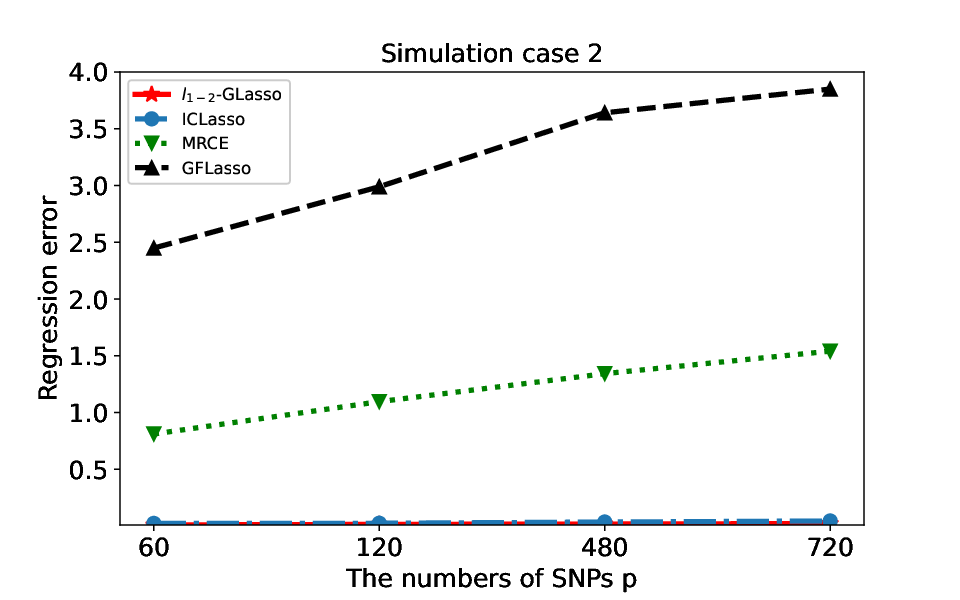
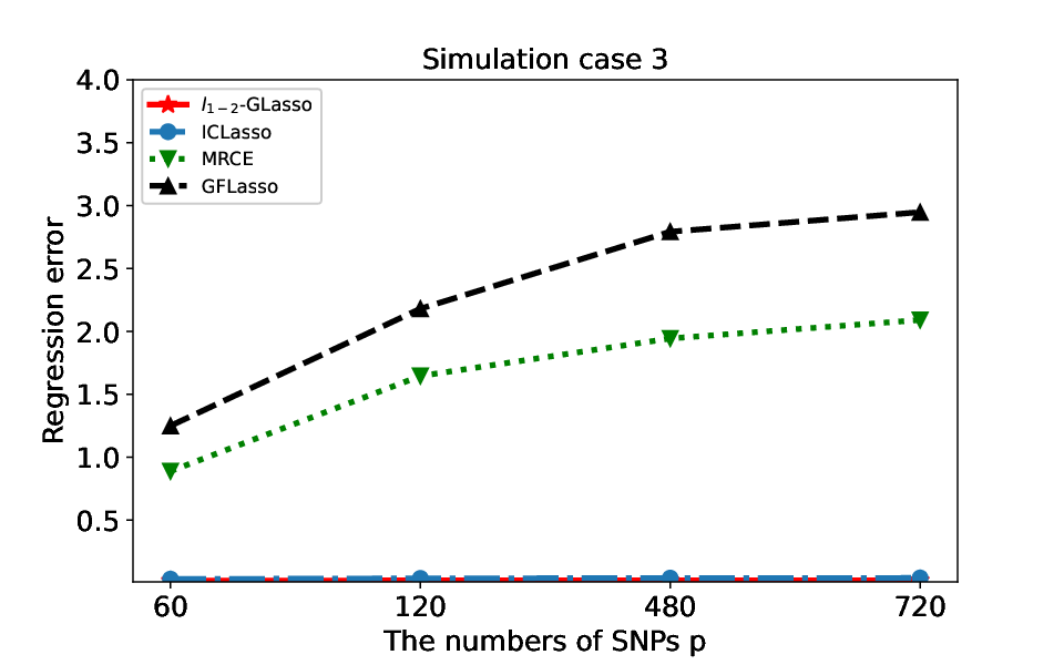
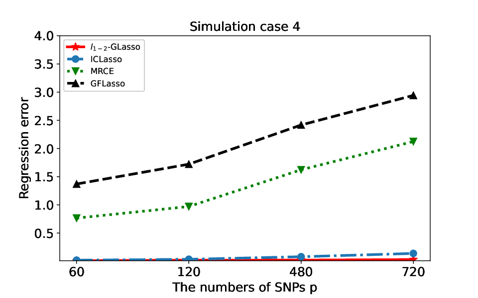
In Figure 3, 4, we present the F1 score in the recovery of and . To some extent, the F1 score reflects the ability of each model to learn the regression coefficient matrix and the output structure. In Figure 5, we show the regression error of . It can be seen that in terms of regression error, -GLasso can be a little better than ICLasso. As shown in these Figures, our results clearly show that -GLasso outperforms other baselines in the four cases we considered.

Finally, because -GLasso introduces a new hyperparameter , we also explore the influence of different hyperparameters on the effect of our model. We use the dataset shown in Figure 1, and the regression error with different ratios is presented in Figure 6. As we can see, when , the regression error is minimized. A larger ratio leads to a more satisfying solution. When , the regression error becomes more and more stable, so we finally select to conduct the following experiments.
5 Real dataset From eQTL Mapping
Greenlaw et al. 2017 analyze a dataset obtained from the ADNI-1 database. We compare -GLasso with other models on this dataset. The genes used in our analysis are listed in Table 1.
| Gene ID | Measurement | Region of interest |
|---|---|---|
| Left_AmygVol | Volume | Amygdala |
| Left_CerebCtx | Volume | Cerebral cortex |
| Left_CerebWM | Volume | Cerebral white matter |
| Left_HippVol | Volume | Hippocampus |
| Left_InfLatVent | Volume | Inferior lateral ventricle |
| Left_LatVent | Volume | Lateral ventricle |
| Left_EntCtx | Thickness | Entorhinal cortex |
| Left_Fusiform | Thickness | Fusiform gyrus |
| Left_InfParietal | Thickness | Inferior parietal gyrus |
| Left_InfTemporal | Thickness | Inferior temporal gyrus |
| Left_MidTemporal | Thickness | Middle temporal gyrus |
| Left_Parahipp | Thickness | Parahippocampal gyrus |
| Left_PostCing | Thickness | Posterior cingulate |
| Left_Postcentral | Thickness | Postcentral gyrus |
| Left_Precentral | Thickness | Precentral gyurs |
The dataset is available for subjects, and among all possible SNPs, we include only those SNPs belonging to the top 15 candidate genes listed on the AlzGene database. The dataset presented here is queried from the most recent genome build as of December 2014, from the ADNI-1 database. After quality control and imputation steps, the genetic dataset used for this study includes SNPs from genes.
We apply -GLasso and other models to discover SNPs that influence the expression levels of genes. This type of study is widely known as an expression quantitative trait locus (eQTL) mapping in the genetics community. It is generally believed that when a genetic variation in the genome such as an SNP perturbs the expression of a gene, the effect propagates through the gene network to influence the expressions of genes in downstream of the pathway. First, we estimate the regression coefficient matrix using 480 samples and then compute the regression error on the remaining 152 samples. As shown in Figure 7, -GLasso produces the smallest regression error. It should be noted that we randomly select 480 samples each time and repeat the sample 10 times. We show the median (red) and the discrete distribution of the regression error on these 10 different datasets.

In the original methodology of Wang et al. 2012, based on biological experiments, 24 SNPs that are highly correlated with 15 genes have been detected. According to the results of biological experiments, we also apply the proposed model to find related SNPs. -GLasso finds 22 SNPs among the determined 24 SNPs and these 22 SNPs are highlighted in Table 5. In addition, we also compared the GFLasso, MRCE, and ICLasso on the dataset with our model in Table 2, 3, 4. The SNPs in bold are selected by each model. It can be seen in Table 4, 5 that -GLasso and ICLasso can both estimate the structure of two larger subnetworks in the gene networks. This has been demonstrated by biological experiments. They show that two SNPs: rs405509 and rs10787010 stand out as being potentially associated with the largest number of ROIs. In Table 6, we show the SNPs associated with genes identified by different models. -GLasso is better than the other models. To show the superiority of -GLasso, we can see from Table 2, 3, 4, GFLasso picks out 14 of the determined 24 SNPs , MRCE picks out 16 of the determined 24 SNPs and ICLasso picks out 17 of the determined SNPs. The experimental results are in line with our assumptions about -GLasso. Compared with other models, -GLasso can more accurately determine the SNPs related to genes.
Back to the sparsity, we compare the regression coefficient matrix calculated by -GLasso with ICLasso. As we can see in Figure 8, the proposed model can get sparser solutions. For example, we set our sights on SNP rs4311. In the real dataset, the SNP rs4311 was detected to have an association with the gene InfParietal (L) (Wang et al. 2012). ICLasso not only finds an association between the SNP rs4311 and the gene InfParietal (L) but also detects that the SNP rs4311 is associated with gene AmygVol (L), CerebCtx (L), LatVent (L), EntCtx (L), Fusiform (L). But in our model, -GLasso calculates the coefficients between SNP rs4311 and gene AmygVol (L), CerebCtx (L), LatVent (L), EntCtx (L), Fusiform (L) that are 0.019947, 0, 0, 0, 0. For genes that are not correlated with an SNP, most regression coefficients calculated by -GLasso are . The result shows that our model achieves sparser solutions compared with ICLasso.


.
| SNP | Number of Phenotype | Phenotype ID(Hemisphere) | ||
|---|---|---|---|---|
| rs4311 | 1 | InfParietal (L) | ||
| rs405509 | 8 |
| ||
| rs666004 | 1 | InfTemporal (L) | ||
| rs1433099 | 1 | CerebCtx (L) | ||
| rs1473180 | 4 | CerebCtx (L) ,EntCtx (L), Fusiform (L), PostCing (L) | ||
| rs1475345 | 1 | Parahipp (L) | ||
| rs1568400 | 1 | Precentral (L) | ||
| rs2149196 | 1 | Postcentral (L) | ||
| rs2418811 | 1 | CerebWM (L) | ||
| rs4935774 | 1 | CerebWM (L) | ||
| rs6107516 | 1 | MidTemporal (L) | ||
| rs6584307 | 1 | Parahipp (L) | ||
| rs11191692 | 1 | EntCtx (L) | ||
| rs12209631 | 2 | CerebCtx (L), HippVol (L) | ||
| rs16924159 | 1 | PostCing (L) | ||
| rs1023024 | 1 | Precentral (L) | ||
| rs1269918 | 3 | CerebCtx (L), CerebWM (L), InfLatVent (L) | ||
| rs2327389 | 1 | AmygVol (L) | ||
| rs2418811 | 1 | CerebWM (L) | ||
| rs2756271 | 4 | EntCtx (L), HippVol (L), InfTemporal (L), Parahipp (L) | ||
| rs7219773 | 1 | Precentral (L) | ||
| rs9314349 | 1 | Parahipp (L) | ||
| rs10787010 | 7 |
| ||
| rs10787011 | 1 | EntCtx (L) | ||
| rs11601726 | 2 | CerebWM (L), LatVent (L) | ||
| SNP | Number of Phenotype | Phenotype ID(Hemisphere) | |
|---|---|---|---|
| rs4311 | 1 | InfParietal (L) | |
| rs405509 | 3 |
| |
| rs666004 | 1 | InfTemporal (L) | |
| rs1433099 | 1 | CerebCtx (L) | |
| rs1473180 | 4 | CerebCtx (L) ,EntCtx (L), Fusiform (L), PostCing (L) | |
| rs1475345 | 1 | Parahipp (L) | |
| rs1568400 | 1 | Precentral (L) | |
| rs2149196 | 1 | Postcentral (L) | |
| rs2327389 | 1 | AmygVol (L) | |
| rs4935774 | 1 | CerebWM (L) | |
| rs6107516 | 1 | MidTemporal (L) | |
| rs6584307 | 1 | Parahipp (L) | |
| rs9314349 | 1 | Parahipp (L) | |
| rs10787010 | 2 |
| |
| rs11191692 | 1 | EntCtx (L) | |
| rs12209631 | 2 | CerebCtx (L), HippVol (L) | |
| rs1023024 | 1 | Precentral (L) | |
| rs1269918 | 3 | CerebCtx (L), CerebWM (L), InfLatVent (L) | |
| rs2418811 | 1 | CerebWM (L) | |
| rs2756271 | 4 | EntCtx (L), HippVol (L), InfTemporal (L), Parahipp (L) | |
| rs7219773 | 1 | Precentral (L) | |
| rs10787011 | 1 | EntCtx (L) | |
| rs11601726 | 2 | CerebWM (L), LatVent (L) | |
| rs16924159 | 1 | PostCing (L) | |
| SNP | Number of Phenotype | Phenotype ID(Hemisphere) | ||
|---|---|---|---|---|
| rs4311 | 1 | InfParietal (L) | ||
| rs405509 | 8 |
| ||
| rs1433099 | 1 | CerebCtx (L) | ||
| rs1473180 | 4 | CerebCtx (L) ,EntCtx (L), Fusiform (L), PostCing (L) | ||
| rs1475345 | 1 | Parahipp (L) | ||
| rs1568400 | 1 | Precentral (L) | ||
| rs2149196 | 1 | Postcentral (L) | ||
| rs2418811 | 1 | CerebWM (L) | ||
| rs4935774 | 1 | CerebWM (L) | ||
| rs6107516 | 1 | MidTemporal (L) | ||
| rs6584307 | 1 | Parahipp (L) | ||
| rs9314349 | 1 | Parahipp (L) | ||
| rs10787010 | 7 |
| ||
| rs10787011 | 1 | EntCtx (L) | ||
| rs11191692 | 1 | EntCtx (L) | ||
| rs12209631 | 2 | CerebCtx (L), HippVol (L) | ||
| rs16924159 | 1 | PostCing (L) | ||
| rs666004 | 1 | InfTemporal (L) | ||
| rs1023024 | 1 | Precentral (L) | ||
| rs1269918 | 3 | CerebCtx (L), CerebWM (L), InfLatVent (L) | ||
| rs2327389 | 1 | AmygVol (L) | ||
| rs2756271 | 4 | EntCtx (L), HippVol (L), InfTemporal (L), Parahipp (L) | ||
| rs7219773 | 1 | Precentral (L) | ||
| rs11601726 | 2 | CerebWM (L), LatVent (L) | ||
| SNP | Number of phenotype | Phenotype ID(Hemisphere) | ||
|---|---|---|---|---|
| rs4311 | 1 | InfParietal (L) | ||
| rs405509 | 8 |
| ||
| rs666004 | 1 | InfTemporal (L) | ||
| rs1023024 | 1 | Precentral (L) | ||
| rs1269918 | 3 | CerebCtx (L), CerebWM (L), InfLatVent (L) | ||
| rs1433099 | 1 | CerebCtx (L) | ||
| rs1473180 | 4 | CerebCtx (L) ,EntCtx (L), Fusiform (L), PostCing (L) | ||
| rs1475345 | 1 | Parahipp (L) | ||
| rs1568400 | 1 | Precentral (L) | ||
| rs2149196 | 1 | Postcentral (L) | ||
| rs2418811 | 1 | CerebWM (L) | ||
| rs2756271 | 4 | EntCtx (L), HippVol (L), InfTemporal (L), Parahipp (L) | ||
| rs4935774 | 1 | CerebWM (L) | ||
| rs6107516 | 1 | MidTemporal (L) | ||
| rs6584307 | 1 | Parahipp (L) | ||
| rs9314349 | 1 | Parahipp (L) | ||
| rs10787010 | 7 |
| ||
| rs10787011 | 1 | EntCtx (L) | ||
| rs11191692 | 1 | EntCtx (L) | ||
| rs11601726 | 2 | CerebWM (L), LatVent (L) | ||
| rs12209631 | 2 | CerebCtx (L), HippVol (L) | ||
| rs16924159 | 1 | PostCing (L) | ||
| rs2327389 | 1 | AmygVol (L) | ||
| rs7219773 | 1 | Precentral (L) | ||
| SNP | GFLasso | MRCE | ICLasso | -GLasso |
| rs4311 | ✘ | ✘ | ✘ | ✘ |
| rs405509 | ✘ | ✘ | ✘ | ✘ |
| rs666004 | ✘ | ✘ | ||
| rs1023024 | ✘ | |||
| rs1269918 | ✘ | |||
| rs1433099 | ✘ | ✘ | ✘ | ✘ |
| rs1473180 | ✘ | ✘ | ✘ | ✘ |
| rs1475345 | ✘ | ✘ | ✘ | ✘ |
| rs1568400 | ✘ | ✘ | ✘ | ✘ |
| rs2149196 | ✘ | ✘ | ✘ | ✘ |
| rs2327389 | ✘ | |||
| rs2418811 | ✘ | ✘ | ✘ | |
| rs2756271 | ✘ | |||
| rs4935774 | ✘ | ✘ | ✘ | |
| rs6107516 | ✘ | ✘ | ✘ | ✘ |
| rs6584307 | ✘ | ✘ | ✘ | ✘ |
| rs7219773 | ||||
| rs9314349 | ✘ | ✘ | ✘ | |
| rs10787010 | ✘ | ✘ | ✘ | |
| rs10787011 | ✘ | ✘ | ✘ | |
| rs11191692 | ✘ | ✘ | ✘ | ✘ |
| rs11601726 | ✘ | |||
| rs12209631 | ✘ | ✘ | ✘ | ✘ |
| rs16924159 | ✘ | ✘ | ✘ | |
| Count | 14 | 16 | 17 | 22 |
6 Conclusion
In this paper, we propose the Graphical Lasso based on difference of and norms, which introduce a new penalty for the sparsity of . Based on two important assumptions, we jointly estimate the regression coefficient matrix and the output structure . Similar to ICLasso, the optimization problem can be solved based on existing algorithms. Through the synthetic dataset, we demonstrate that -GLasso outperforms other models in the recovery of the eQTL associations and the gene network structure. The results on real datasets also show the superiority of -GLasso and confirm the assumptions of the model. Also, we can use other penalty norm for and , like penalty which is closer to the penalty. Future work will seek higher efficiency of the solution algorithm and decomposition of large-scale problems. The application domain of this model can also be extended to financial data.
References
- Bertsimas and Van Parys (2020) [author] Bertsimas, DimitrisD. and Van Parys, BartB. (2020). Sparse high-dimensional regression: Exact scalable algorithms and phase transitions. The Annals of Statistics 48 300–323.
- Chun et al. (2013) [author] Chun, HyonhoH., Chen, MinM., Li, BingB. and Zhao, HongyuH. (2013). Joint conditional Gaussian graphical models with multiple sources of genomic data. Frontiers in Genetics 4 294.
- Esser, Lou and Xin (2013) [author] Esser, ErnieE., Lou, YifeiY. and Xin, JackJ. (2013). A method for finding structured sparse solutions to nonnegative least squares problems with applications. SIAM Journal on Imaging Sciences 6 2010–2046.
- Friedman, Hastie and Tibshirani (2008) [author] Friedman, JeromeJ., Hastie, TrevorT. and Tibshirani, RobertR. (2008). Sparse inverse covariance estimation with the graphical lasso. Biostatistics 9 432–441.
- Gardner and Faith (2005) [author] Gardner, Timothy ST. S. and Faith, Jeremiah JJ. J. (2005). Reverse-engineering transcription control networks. Physics of Life Reviews 2 65–88.
- Greenlaw et al. (2017) [author] Greenlaw, KeelinK., Szefer, ElenaE., Graham, JinkoJ., Lesperance, MaryM., Nathoo, Farouk SF. S. and Initiative, Alzheimer’s Disease NeuroimagingA. D. N. (2017). A Bayesian group sparse multi-task regression model for imaging genetics. Bioinformatics 33 2513–2522.
- Hoyer (2004) [author] Hoyer, Patrik OP. O. (2004). Non-negative matrix factorization with sparseness constraints. Journal of Machine Learning Research 5.
- Kim and Xing (2009) [author] Kim, SeyoungS. and Xing, Eric PE. P. (2009). Statistical estimation of correlated genome associations to a quantitative trait network. PLoS Genetics 5 e1000587.
- Kim and Xing (2012) [author] Kim, SeyoungS. and Xing, Eric PE. P. (2012). Tree-guided group lasso for multi-response regression with structured sparsity, with an application to eQTL mapping. The Annals of Applied Statistics 6 1095–1117.
- Li, Chun and Zhao (2012) [author] Li, BingB., Chun, HyonhoH. and Zhao, HongyuH. (2012). Sparse estimation of conditional graphical models with application to gene networks. Journal of the American Statistical Association 107 152–167.
- Li and Gui (2006) [author] Li, HongzheH. and Gui, JiangJ. (2006). Gradient directed regularization for sparse Gaussian concentration graphs, with applications to inference of genetic networks. Biostatistics 7 302–317.
- Liu et al. (2016) [author] Liu, ChanziC., Chen, QingchunQ., Zhou, BingpengB. and Li, HengchaoH. (2016). - and -Norm Joint Regularization Based Sparse Signal Reconstruction Scheme. Mathematical Problems in Engineering 2016.
- Marbach et al. (2010) [author] Marbach, DanielD., Prill, Robert JR. J., Schaffter, ThomasT., Mattiussi, ClaudioC., Floreano, DarioD. and Stolovitzky, GustavoG. (2010). Revealing strengths and weaknesses of methods for gene network inference. Proceedings of the National Academy of Sciences 107 6286–6291.
- Marchetti-Bowick et al. (2019) [author] Marchetti-Bowick, MicolM., Yu, YaoliangY., Wu, WeiW. and Xing, Eric PE. P. (2019). A penalized regression model for the joint estimation of eQTL associations and gene network structure. The Annals of Applied Statistics 13 248–270.
- Meinshausen and Bühlmann (2006) [author] Meinshausen, NicolaiN. and Bühlmann, PeterP. (2006). High-dimensional graphs and variable selection with the lasso. The Annals of Statistics 34 1436–1462.
- Michaelson et al. (2010) [author] Michaelson, Jacob JJ. J., Alberts, RudiR., Schughart, KlausK. and Beyer, AndreasA. (2010). Data-driven assessment of eQTL mapping methods. BMC Genomics 11 1–16.
- Peng et al. (2009) [author] Peng, JieJ., Wang, PeiP., Zhou, NengfengN. and Zhu, JiJ. (2009). Partial correlation estimation by joint sparse regression models. Journal of the American Statistical Association 104 735–746.
- Rockman and Kruglyak (2006) [author] Rockman, Matthew VM. V. and Kruglyak, LeonidL. (2006). Genetics of global gene expression. Nature Reviews Genetics 7 862–872.
- Rothman, Levina and Zhu (2010) [author] Rothman, Adam JA. J., Levina, ElizavetaE. and Zhu, JiJ. (2010). Sparse multivariate regression with covariance estimation. Journal of Computational and Graphical Statistics 19 947–962.
- Schäfer and Strimmer (2005) [author] Schäfer, JulianeJ. and Strimmer, KorbinianK. (2005). A shrinkage approach to large-scale covariance matrix estimation and implications for functional genomics. Statistical Applications in Genetics and Molecular Biology 4.
- Segal et al. (2005) [author] Segal, EranE., Friedman, NirN., Kaminski, NaftaliN., Regev, AvivA. and Koller, DaphneD. (2005). From signatures to models: understanding cancer using microarrays. Nature Genetics 37 S38–S45.
- Tibshirani (1996) [author] Tibshirani, RobertR. (1996). Regression shrinkage and selection via the lasso. Journal of the Royal Statistical Society: Series B (Methodological) 58 267–288.
- Vinga (2021) [author] Vinga, SusanaS. (2021). Structured sparsity regularization for analyzing high-dimensional omics data. Briefings in Bioinformatics 22 77–87.
- Wang et al. (2012) [author] Wang, HuaH., Nie, FeipingF., Huang, HengH., Kim, SungeunS., Nho, KwangsikK., Risacher, Shannon LS. L., Saykin, Andrew JA. J., Shen, LiL. and Initiative, Alzheimer’s Disease NeuroimagingA. D. N. (2012). Identifying quantitative trait loci via group-sparse multitask regression and feature selection: an imaging genetics study of the ADNI cohort. Bioinformatics 28 229–237.
- Wang et al. (2019) [author] Wang, LingqianL., Zhou, HuiH., Wang, YufengY., Yu, BoB., Zhang, YuanpengY., Liu, WenlingW. and Chen, YangkangY. (2019). Three-parameter prestack seismic inversion based on minimization. Geophysics 84 R753–R766.
- Yin, Esser and Xin (2014) [author] Yin, PenghangP., Esser, ErnieE. and Xin, JackJ. (2014). Ratio and difference of and norms and sparse representation with coherent dictionaries. Communications in Information and Systems 14 87–109.
- Yin and Li (2011) [author] Yin, JianxinJ. and Li, HongzheH. (2011). A sparse conditional Gaussian graphical model for analysis of genetical genomics data. The Annals of Applied Statistics 5 2630.
- Yin et al. (2015) [author] Yin, PenghangP., Lou, YifeiY., He, QiQ. and Xin, JackJ. (2015). Minimization of for compressed sensing. SIAM Journal on Scientific Computing 37 A536–A563.
- Yu (2013) [author] Yu, Yao-LiangY.-L. (2013). Better approximation and faster algorithm using the proximal average. Advances in Neural Information Processing Systems 26.
- Yuan and Lin (2006) [author] Yuan, MingM. and Lin, YiY. (2006). Model selection and estimation in regression with grouped variables. Journal of the Royal Statistical Society: Series B (Statistical Methodology) 68 49–67.