The IXPE view of GRB 221009A
Abstract
We present the IXPE observation of GRB 221009A which includes upper limits on the linear polarization degree of both prompt and afterglow emission in the soft X-ray energy band. GRB 221009A is an exceptionally bright gamma-ray burst (GRB) that reached Earth on 2022 October 9 after travelling through the dust of the Milky Way. The Imaging X-ray Polarimetry Explorer (IXPE) pointed at GRB 221009A on October 11 to observe, for the first time, the 2–8 keV X-ray polarization of a GRB afterglow. We set an upper limit to the polarization degree of the afterglow emission of 13.8% at a 99% confidence level. This result provides constraints on the jet opening angle and the viewing angle of the GRB, or alternatively, other properties of the emission region. Additionally, IXPE captured halo-rings of dust-scattered photons which are echoes of the GRB prompt emission. The 99% confidence level upper limit to the prompt polarization degree depends on the background model assumption and it ranges between to . This single IXPE pointing provides both the first assessment of X-ray polarization of a GRB afterglow and the first GRB study with polarization observations of both the prompt and afterglow phases.
Keywords:
GRB — X-ray — polarizationI Introduction
Gamma-Ray Bursts (GRBs) are among the most energetic events in the Universe. These events are characterized by a “prompt” gamma-ray emission, the most luminous phase of the burst, followed by a temporally decaying “afterglow” that can last for days or even years and is observed across the whole electromagnetic spectrum whenever the needed sensitivity is available. GRBs are conventionally classified by duration of the prompt phase into the short ( sec) and long ( sec) class, with distinct physical origins (Galama et al. 1998; Abbott et al. 2017; Fong et al. 2015; Burns et al. 2021). Long GRBs originates from collapsars (Woosley & Bloom 2006), a rare sub-type of type Ic supernovae. In the standard model, a fast spinning core collapses into a rapidly spinning black hole which devours some of the massive star progenitor. This results in a hyper-accreting process that powers bipolar, ultrarelativistic, collimated jets which ultimately release the prompt GRB signature (Kumar & Zhang 2015). Despite detecting more than 10,000 GRBs in their prompt phase, our understanding of these events and the underlying physical processes is still limited (Zhang 2018). We also notice that in the X-Ray band covered by IXPE (28 keV), measurements of the prompt emission are meager. In fact, our knowledge relies on less than 100 detections by BeppoSAX and HETE-2 (Frontera 2019; Costa & Frontera 2011; Tamagawa et al. 2003, see, e.g.,).
Advances in understanding require new diagnostics, e.g. observations of polarization or multiple messengers. However, so far, only upper limits on neutrino emission from either prompt or early-afterglow emission have been set, suggesting a leptonic composition of the jet bulk (Abbasi et al. 2022). Only a few GRBs (before GRB 221009A) have been detected in the very-high-energy regime and only one (short GRB) coincident with gravitational waves (Abbott et al. 2017). Polarization measurements of the prompt emission of GRBs can represent a unique observable to constrain the outflow composition and dynamics, to determine the structure of the magnetic fields at the jet formation, and provide insights on the radiation mechanisms behind the observed GRB spectra as well as on our viewing angle within the jet opening angle (see, e.g., Gill et al. 2021, for a recent overview). Thus far, GRB polarization observations in the prompt phase have only occurred in the hard X-ray / soft gamma-ray band, reporting generally high polarization degrees, but never an unambiguous detection (see, e.g., McConnell 2017, for a critical review). The largest catalog of prompt GRB gamma-ray polarization measurements comes from the POLAR mission, with 14 observations but no clear detection. The picture is further complicated because the time-integrated polarization seems to be affected by polarization angle swing in time (Kole et al. 2020). The forthcoming POLAR-2 (Hulsman 2020) and COSI (Tomsick et al. 2021) missions are designed for significantly larger detection catalogs, as is the proposed LEAP mission (McConnell et al. 2021).
After the prompt emission the jet propagates and interacts with the ambient medium, developing a shock, where electrons are accelerated and produce synchrotron emission, referred to as afterglow, throughout the whole electromagnetic spectrum, from radio to very-high energy gamma-rays. Observations of polarization in the afterglow phase can also provide insight into jet physics and structure (Rossi et al. 2004). Models in the literature (Kuwata et al. 2022) predict a progressive loss of coherence of the propagating jet magnetic fields, which results in an expected low polarization degree (below 5–3%) of the late-phases of the GRB afterglow emission. These predictions are largely consistent with results from time-resolved GRB afterglow measurements of optical polarization (Mundell et al. 2013; Covino & Gotz 2016; Stringer & Lazzati 2020). Radio polarization measurements typically show a lower polarization degree than do the optical measurements (Urata et al. 2019; Urata et al. 2022), motivating an increasing interest in a multiwavelength modeling of late-afterglow polarization (Shimoda & Toma 2021; Birenbaum & Bromberg 2021). No observations of afterglow polarization have been reported so far at X-ray energies.
On 2022 October 9 an exceptionally bright transient event outshone the rest of the high-energy sky. The first trigger was recorded in the gamma-ray band by the Fermi Gamma-ray Burst Monitor (GBM) at 13:16:59.988 UTC (Veres et al. 2022; Lesage et al. 2022), and the same event was also strongly detected by the Fermi Large Area Telescope (LAT) up to a hundred GeV (Pillera et al. 2022). The Large High Altitude Air Shower Observatory (LHAASO) also reported the detection of gamma-rays up to 18 TeV (Huang et al. 2022). After about an hour from the initial trigger, as soon as the source was observed, the Burst Alert Telescope on board of the Neil Gehrels Swift Observatory triggered on the same event and the Swift X-Ray Telescope (XRT)(Burrows et al. 2005) was on target 143 seconds later and the Swift Ultraviolet/Optical Telescope (UVOT) located it at (RA(J2000), DEC(J2000)) = (288.26452∘, 19.77350∘) with a 90%-confidence error radius of about 0.61 arcsec (Dichiara et al. 2022). The event, soon classified as a gamma-ray burst (Veres et al. 2022), happened at a redshift of 0.151 as reported by X-shooter/VLT (Ugarte Postigo et al. 2022), and is the brightest (at Earth) ever recorded by any gamma-ray burst monitor by a large margin. Furthermore, the detection of dust-scattered soft X-ray rings was reported (Tiengo et al. 2022) through Swift/XRT observations in the two days after the prompt emission. Such rings are produced by X-rays from the extremely bright prompt emission efficiently scattered at small angles by interstellar dust grains in our Galaxy (Miralda-Escudé 1999, e.g.,). The scattered X-rays are delayed with respect to direct ones, due to their longer path length from the source to the observer, with a delay that depends on the distance of the dust cloud traversed by the X-ray radiation. Thus, the rings are echoes of the prompt emission.
The Imaging X-ray Polarimetry Explorer (IXPE) is a space observatory with three identical telescopes designed to measure the polarization of astrophysical X-rays (Weisskopf et al. 2022; O’Dell et al. 2019; Soffitta et al. 2020). Launched on 2021 December 9, IXPE is an international collaboration between NASA and the Italian Space Agency (ASI), and it has been operating since January of 2022. IXPE measures polarization using the photo-electric effect of X-rays absorbed in the gas gap of a Gas Pixel Detector (GPD) (Bellazzini et al. 2006). On 2022 October 11 at 23:35:35.184 UTC IXPE started the observation of GRB 221009A in response to a Target of Opportunity request (Negro et al. 2022). The location position was provided by a Swift/UVOT observation (Dichiara et al. 2022). The observation ended on 2022 October 14 at 00:46:44.184 UTC with an effective exposure of 94,122 s.
In this work we present the results of the IXPE observation carried out with the fully processed data and through a careful data analysis. This represents the first observation of X-ray polarization of a GRB afterglow, the first measurement of soft X-ray polarization of GRB prompt emission, and the first time we observe polarization properties in both prompt and afterglow phases of the same GRB.
After a brief general introduction on IXPE data analysis provided in Section II, we devote Section III to the data analysis and interpretation of the GRB afterglow emission, while Section IV illustrates the data analysis and interpretation of the rings in association to the GRB prompt emission. Summary and conclusions are offered in Section V.
II IXPE Polarization Analysis
We analyze IXPE Level 2 processed data11 1 IXPE data are publicly available on the HEASARC archive., combining the data collected by the three identical detector units (DUs). The time-integrated radial profile reveals inconsistency with the expectation from a point-like source, showing a profile that deviates from the instrument point spread function (PSF). In particular two excesses around the peak emission are visible (see Figure 7 and Figure 10 in the Appendix). Such excess appears as rings around a bright core emission and are associated with dust-scattering halos (Hayakawa 1970; Miralda-Escudé 1999, e.g.,). To utilize the full potential of this observation an image- and time-resolved analysis has been carried out, as described in the next section.
Prior to the data analysis, we perform a first background rejection removing a fraction of background events, mostly composed of cosmic rays interacting in the sensitive area of the instrument. A residual cosmic-ray background component still remains and needs to be estimated and subtracted from the data as well. The correct modeling of such a component is particularly relevant to study the fainter extended emission of the dust-scattering rings. As a suitable background region cannot be extracted directly from this observation, due to the presence of the rings, we assess the expected X-ray background rate from previous IXPE observations. In particular, we consider three IXPE observations of low-rate point-like sources: the observation of 1ES 1959+650 carried out between 2022 June 9 and 2022 June 12 (BKG1); the observation of BL Lacertae (BL Lac) which happened between 2022 July 7 and 2022 July 09 (BKG2); the observation of 3C 279 performed between 2022 June 12 and 2022 June 18 (BKG3). From each of these observations we extract the background spectrum and we simulate a long exposure (1 Ms) IXPE observation with the ixpeobssim simulation tool (Baldini et al. 2022). The three selected observations provide a good bracketing of the background emission. More details on the particle background rejection, the residual background simulation, scaling, and subtraction are reported in Appendix A.
Typically, for IXPE observations, the polarization information is extracted via two types of analyses: a polarimetric analysis and a spectropolarimetric analysis. For the former, we use the xpbin routine of ixpeobssim with the flag --algorithm PCUBE. This routine computes the I-normalized Stokes parameters Q and U from the event-by-event Stokes parameters of the sample of selected events. The algorithm supports the calculation of the background-subtracted Stokes parameters, if a background template is provided. The polarization degree (PD) and polarization angle (PA) with associated errors are calculated from the Q/I and U/I parameters following the recipe of Kislat et al. 2015.
The spectropolarimetric analysis, as opposed to the simpler polarimetric analysis, accounts for the shape of the intensity spectrum. This analysis consists of the joint fit of the I, Q and U spectra and, for this work, we make use of the Multi-Mission Maximum Likelihood (3ML) framework 22 2 https://threeml.readthedocs.io/en/stable/index.html (Vianello et al. 2015), which is publicly available and allows for both frequentist and Bayesian analysis approaches. Here we report the results of the frequentist analysis, but we verified that the Bayesian approach leads to the same results.
Hereafter, we refer to the central region as the core, while the inner and the outer rings are denoted r1 and r2, respectively. In the next sections we will illustrate the data analyses and results for these different regions.
III The Core / Afterglow emission
III.1 Data analysis


We start with the analysis of the core, which arises from the burst afterglow. We select the region as a disc centered on the brightest pixel33 3 The image pixel size is . of the IXPE image and radius of 26 arcsec (0.43 arcmin). Beyond this radius, the radial profile of the emission deviates from the PSF of the instrument by more than 20%, as shown in Figure 1 (left panel). Such a deviation informs us on possible contamination from the emission of dust-scattered X-rays (from the GRB prompt and/or afterglow emission) that we cannot fully resolve. We verified that the bright core emission from the central point-like source dominates the final result as we find consistent numbers within the one sigma uncertainty when varying slightly the selecting radius. According to the IXPE PSF, cutting at a radius of 26 arcsec eliminates less than 15% of the total source emission.
Given the high photon statistics of the core (signal-to-noise ratio for any background), the results of the analysis are not affected by the choice of the background spectrum. Here, we report the results for the background template BKG2. Through the PCUBE analysis, we find an unconstrained polarization in the 2–8 keV energy range and derive a 99% C.L. upper limit of 16.1%. No evolution with time or energy is observed. For the spectropolarimetric analysis we model the observed spectrum with an absorbed power law decreasing in energy, with intrinsic parameters fixed to the values of the Swift/XRT automated online analysis (Evans et al. 2007), which are consistent with other reported values (Kennea et al. 2022). In particular, the intrinsic absorption parameters are fixed to cm-2 (Evans et al. 2007) at a redshift of 0.151 (Ugarte Postigo et al. 2022), while the Galactic absorption value is fixed to cm-2 (Willingale et al. 2013). To account for mismatches of inter-calibration among the different IXPE telescopes, a constant normalization is left free to vary for DU2 and DU3 with respect to DU1.
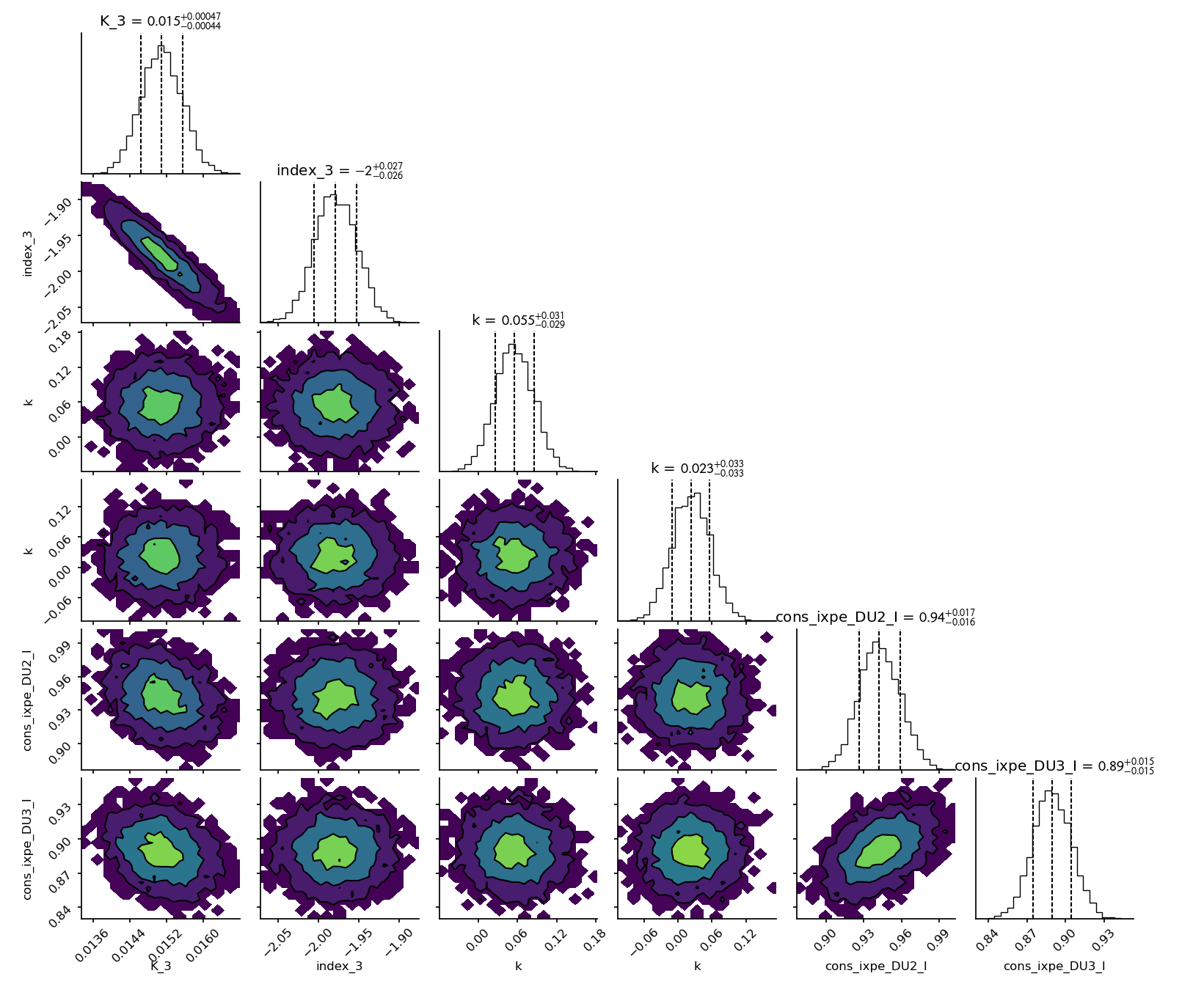
The best-fit values of the spectropolarimetric analysis are provided in Table 1. We find a best-fit power-law index of , in agreement with expectations from a late afterglow emission (see Section III.2). The polarization results are slightly more constraining than, but consistent with, the PCUBE analysis with a polarization degree of . The right panel of Figure 1 shows the Q/I versus U/I distribution of the core emission.
The Stokes parameters Q/I and U/I are expected to be normally distributed with respective means and , and equal standard deviations. An error contour in (Q/I, U/I) space is a circle of radius centered on (), where is distributed as (d.o.f=2). The probability that the observed polarization exceeds the measured value, under the null hypothesis of unpolarized emission, is 9.7%. This is inconsistent with a zero degree of polarization at 90% C.L. We therefore set a upper limit to the polarization degree (1D distribution) of 13.8% at 99% C.L. (12.1% at 95% C.L.). For completeness, the I, Q, U spectra are reported in Figure 12 (first row) in Appendix B.3.
| Parameter | Value |
|---|---|
| PD | ()% |
| PD U.L. 99% C.L. | |
| PD U.L. 95% C.L. | |
Note. — Summary table of the spectropolarimetric analysis of the core. The spectropolarimetric fit is performed in the 2–8 keV energy band and it assumes Gaussian statistics. The PA is unconstrained. The best-fit Q/I and U/I constants are and , respectively.
III.2 Interpretation
According to current models, once beyond the early flaring stages, GRB afterglows arise via synchrotron processes from electrons accelerated through interactions of the GRB jet with the circumstellar material. This is consistent with observations from radio to high energies of GRB afterglows (Kumar & Zhang 2015). The physics is well understood and follows a set of closure relations (Sari & Mészáros 2000, e.g.,) which, when observations fit a self-consistent picture, can be used to infer properties of the underlying emitting region through observables such as the spectral indices and rate of temporal decay. The synchrotron spectrum is described by a set of power laws with different spectral indices, each with its own closure relation depending on the particle density distribution of the circumstellar environment. We model the core X-ray emission as observed by IXPE with this interpretation, in order to utilize the polarimetric observation to constrain intrinsic properties of the jet and our viewing angle.
We start by investigating the density of the interstellar matter around the GRB progenitor. The density profile in units of cm-3, , where is the distance from the central engine, is parameterized by the index , such that . For example, corresponds to a constant density medium and describes a wind medium, and in-between values are also possible. A wind medium may be expected around long GRBs since they arise in the deaths of massive stars. The density profile affects the time evolution of the synchrotron break frequencies. We assume that the IXPE energy range lies between the typical () and the cooling () synchrotron frequencies, and show that this assumption yields a consistent picture.
The time and energy evolution of GRB afterglow emission is described by (Granot & Sari 2002, see, e.g.,)
| (1) |
The core spectrum is well fit by an absorbed power law with a photon index of , which yields . The temporal evolution of GRB afterglow usually shows a break, which causes the index to increase. This steepening is proportional to , where is the jet Lorentz factor and the jet half opening angle. Taking into account the time evolution of the Lorentz factor, the increase in the temporal index will be . From the closure relations (Sari & Mészáros 2000, e.g.,) between the temporal and spectral indices, we can express the index of the density profile as
| (2) |
For , measured by Swift-XRT44 4 Swift-XRT data were analyzed in the IXPE observation time window through the online tool: https://www.swift.ac.uk/xrt_live_cat/01126853/. IXPE’s light curve shows a consistent time evolution, but we find a less precise estimation of the power index. Therefore, we adopt the Swift value in our model. and , we get . We note that using the Swift-XRT spectral index of , we get . In our model we assume that the IXPE observation was preceded by an achromatic jet break at 1 day (D’Avanzo et al. 2022).
We will thus assume that the forward shock propagates in a wind medium with density , where . To estimate we introduce fiducial or base values for the energy density fraction in electrons and in magnetic fields:
| (3) |
Furthermore, we set the kinetic energy of the outflow to erg and we use the scaling convention for quantity in cgs units. With the above choice of parameters, and neglecting the effect of inverse Compton scattering on the cooling, we have (Granot & Sari 2002, e.g.,):
| (4) |
confirming that indeed at the time of the IXPE observation, and this ordering persists at later times because and . In this spectral regime, the energy spectral index is given by , where p is the power law index of the electron energy distribution (, where is the electron’s Lorentz factor). Using the derived from IXPE observation, we find .
We can now estimate by comparing the observed flux density at 10 keV, Jy, to the synchrotron model prediction (Granot & Sari 2002, e.g.,), valid after the jet break:
| (5) |
We note that depends strongly on the parameter ( for ).
A separate constraint for our afterglow model comes from the measured jet break time, , which scales as if the ratio between the jet opening angle and viewing angle is known. This parameter, and its position in time with respect to the time of the observation, is relevant for polarization, as it can be broadly associated with the time when the polarization degree lightcurve has a zero point and the polarization angle rotates by 90 degrees. In fact, for uniform (top-hat) jet structure with no sideways expansion, significant polarization arises from the break in symmetry of the visible surface. This surface is typically an annulus when projected to the plane of the sky. As the annulus grows, it encompasses a progressively larger fraction of the jet surface. Eventually, for an off-axis observer, the annulus will grow beyond the size of the jet on one side, while still collecting emission from the opposite side, resulting in net polarization. The polarization lightcurve exhibits the typical two-bump structure (Ghisellini & Lazzati 1999; Sari 1999), where the jet break time approximately corresponds to the minimum between the bumps. Our model is constructed so that the PD zero point between the two bumps is at day, to match the estimated jet break time (D’Avanzo et al. 2022). We derive the expected polarization degree by integrating the intensity and polarization of the comoving volume elements of the jet over the equal arrival time surfaces (Sari 1999; Granot & Königl 2003; Shimoda & Toma 2021; Pedreira et al. 2022). For each comoving volume element, the maximum PD of a synchrotron-emitting, shock accelerated electron population with power-law distribution with index will be: (Rybicki & Lightman 1979). The observed polarization will be reduced from this value by integrating over all the parts of the jet that contribute to the flux at a given observer time (Lyutikov et al. 2003, see e.g.,).
The evolution of the polarization as a function of time depends strongly on a variety of parameters. We take a set of parameters (base values) that give a polarization consistent with the IXPE spectropolarimetric measurement: jet opening angle deg, viewing angle (Ghisellini & Lazzati 1999), electron energy distribution index p=2.96, kinetic energy erg, density parameter cm-1 and . The parameter is the ratio of the magnetic field strength in two directions defined as: . Here, and are the magnetic field parallel and perpendicular to the shock normal, respectively. The case yields the maximum attainable polarization for any given set of afterglow parameters. Our model with base values and several additional realizations is presented in Figure 2. In general terms, all realizations have zero points anchored at day and yield increasing PD at the time of the IXPE observations. For a given ratio, we can choose a set of parameters (, and ) so that day is satisfied. A higher ratio results in a higher peak polarization and earlier jet break time, due to the higher level of asymmetry as we move away from the jet axis.
All presented models in Figure 2, except the low jet opening angle, are consistent with the upper limit. Taking the PD= at face value, models with jet opening angle deg (while keeping all other base values fixed) are disfavored. Similarly, models with tend to overpredict the IXPE measurement. Assuming a magnetic field ratio, , closer to 1 simply scales down the PD. In principle, any model that overpredicts the observations can be made consistent by appropriate choice of . The IXPE measurement, considering the base values, favors cases where .
Optical polarization observations occurred during the IXPE observation window at the Nordic Optical Telescope (Lindfors et al. 2022). The sky conditions allowed an estimation of an upper limit to the optical polarization degree of 8.3% at 99% C.L. (Lindfors et al. 2022, 5.1% at 95% C.L., ). In Appendix B.1 we provide more details about the optical data reduction. The optical band falls in the same spectral regime as the X-rays () for most choices of parameters around the base values. Thus the optical upper limit can be used to constrain the models. The optical limit is slightly stronger, but gives qualitatively the same constraints as the X-ray limit. As the above analysis assumes a homogeneous jet (top-hat profile), more elaborate profiles —e.g., Gaussian jet or structured jet (Rossi et al. 2004)— could give different results.
IV The Rings / Prompt emission
IV.1 Data Analysis


As mentioned in the introduction, the observed rings are the result of a known effect involving Galactic dust along the line-of-sight of a bright transient event. A fraction of the photons emitted in the prompt phase of the GRB are scattered by dust clouds in the Milky Way. Those scattered inwards towards the line of sight arrive at Earth after traveling a longer path length with respect to the unscattered ones. This results in a later arrival time of the scattered photons, with a delay that depends on the distance of the dust cloud to Earth and the scattering angle . The angular size of the halos is related to the scattering angle, as , where is the ratio between the distance of the cloud and the distance of the source. Since we are dealing with a transient event at cosmological distance (), the approximation applies (Miralda-Escudé 1999; Draine 2003a).
Being produced by a short transient event, the rings expand radially in time. This arises as photons with different scattering angles travel different path lengths. In order to study the radial evolution of the rings and correctly select prompt, scattered photons as the rings expand, we devise a method inspired by the procedure described in Tiengo & Mereghetti 2006. For each photon detected at a time and at a sky coordinate (, ), we define the following variables
| (6) |
where (, ) are the coordinates of the unscattered emission (the center of the core in the IXPE image) and is the angular distance (in arcsec) of the photon from the point (, ). The trigger time of the prompt emission is taken from the Fermi/GBM55 5 The time difference between the GBM trigger and the beginning on the IXPE observation is 209848 s. Fermi-GBM triggered on a precursor event, about 210 s before the main brighter peak. We reasonably assume that the rings emission is an echo of the brightest part of the prompt phase. Hence we use the GBM trigger time plus 210 seconds. In any case, a difference of 210 seconds on the total time-distance between IXPE observation and the GBM trigger does not affect our results. (Veres et al. 2022). The advantage of this approach is that in the plane vs , shown in the left panel of Figure 3, the expanding rings appear as horizontal bands, facilitating the event selection. We remove the dominant emission from the core by removing events within 0.85 arcmin from the center to avoid contamination from the bright core (afterglow) emission. We estimate that the contamination from the core emission at radial distances larger than 0.85 arcmin is less than 4%. The distribution , after subtracting the simulated background events, is shown in the right panel of Figure 3: the contribution of the two rings is prominent. We fit the distribution around the peaks with the sum of two Lorentzian functions, which approximate well the observed distribution.
We define the event selection cut on the distribution as illustrated in Figure 3 (right panel). The area under each best-fit Lorentzian between R and R (orange areas in the plot), where denotes r1 and r2 respectively, is at least a factor of twenty larger than the area under the other Lorentzian in the same range (gray areas in the plot). This ensures a negligible contamination from the emission of one ring onto the other. The edges of the selection for the wider ring are symmetric with respect to the peak, while the innermost edge of the smaller ring is naturally defined by our region cut off at 0.85 arcmin to exclude the core emission.


Similar to the core analysis, we proceed with the PCUBE polarization analysis in the 2–8 keV energy band. The observed spectra of the two rings are expected to be different because they are generated from the same prompt emission scattered at different angles. As discussed later on, given a scattering angle, the scattering efficiency of X-rays by dust grains is energy dependent (Draine 2003b). This leads to the realization that combining the two ring selections into one single PCUBE analysis would be inaccurate. Furthermore, the low statistics of the individual ring selections prevents a proper background template subtraction for the PCUBE analysis. This implies that the estimated uncertainties are not accurate because they are computed on a boosted statistic that includes background events. The results of the PCUBE analysis for the individual rings are reported in Table 4 of Appendix B.3. We find a PD% and PD%, in agreement with each other. These values indicate a higher polarization degree than what observed in the core, though never exceeding the 99% C.L. required to claim a detection.66 6 The minimum detectable polarization at 99% C.L. (for non background subtracted data) is and for r1 and r2, respectively
The spectropolarimetric fit, allowing a proper combination of the rings selections, can give a more accurate estimation of the underlying polarization. The phenomenological model we define to describe the rings emission allows for the spectral parameters of the rings to be different while sharing common polarization parameters. The spectra of both rings are modeled as absorbed simple power laws, while we assume constant polarization parameters. The intrinsic and Galactic absorption parameters are kept fixed to the same values adopted for the core analysis. As opposed to the PCUBE analysis, we perform the subtraction of the background spectrum. We test different background assumptions, subtracting the spectra derived from BKG1, BKG2, and BKG3 templates, to which we applied the analogous event selection as for r1 and r2.
The results are summarized in Table 2. We find that r1 has a best-fit photon index, averaged over the values obtained assuming different backgrounds, , with a relative statistical error of about 7% and negligible systematic uncertainty due to the choice of the background spectrum. r2 has a steeper spectrum, with photon index with a relative statistical error of about 6% as well as a 7% relative systematic error associated with different background assumptions. This is also illustrated in Figure 14 in Appendix B.3. As we will discuss in the next section, such a difference in spectral index between the two rings is expected owing to the energy dependence of the X-ray scattering cross section. We note that, for the case of r2, the estimated photon index found assuming BKG1 shows a larger statistical error: the softer spectrum of the emission from this ring with respect to r1 makes the measurement more sensitive to the spectral characteristics of the subtracted background (Figure 8 in Appendix B.3 shows that BKG1 has the hardest spectrum).
As for the polarization, we find that the PD value and uncertainty depend upon the assumed background. The statistical-error-weighted average is ()%, where the statistical error is the average among the statistical uncertainties obtained assuming different backgrounds, and the systematic uncertainty is given by the variation of the best-fit value assuming different backgrounds. Figure 4 shows the results for the different background subtractions. The significance of this result, tested against the null hypothesis of unpolarized emission, is about 81% C.L.. The 1D 99% C.L. upper limit on the PD varies between 54.6% and 81.5%, depending on the assumed background. Such a difference is due to the low-statistic regime we have for the rings data selection, which causes the statistical uncertainty to be strongly affected by small changes of the subtracted background.
The comparison of the best-fit PDs found assuming different backgrounds is illustrated in the right plot of Figure 4. For completeness, the Q/I versus U/I distributions obtained for the different assumed background are provided in Figure 15 in Appendix B.3. Note that, given the different approaches and handling of the background, the PCUBE and spectropolarimetric analyses are not directly comparable in this case.
| Summary table of the rings analysis | |
|---|---|
| PD (BKG1) | )% |
| PD (BKG2) | )% |
| PD (BKG3) | )% |
| PDave | % |
| PD U.L. 99% C.L. | |
| PD U.L. 95% C.L. | |
Figure 15 in Appendix B.3 reports the Q/I versus U/I plots for the different background assumptions. Additionally, we show in the same figure the equivalent plots for the spectropolarimetric fit of the individual rings. Furthermore, Figure 11 and Table 4 report the results of the PCUBE analysis of the individual rings resolved in two logarithmic energy bins between 2 and 8 keV. We refer the reader to the Appendix for further discussion on this matter.
IV.2 Interpretation
As discussed in Draine 2003b, the effect of the dust scattering at such a small angles is not expected to alter the intrinsic polarization of the incoming radiation (see their Figure 5). However, an explicit demonstration of this statement in the X-ray band is not directly discussed in the literature. Therefore we investigated the effect on polarization from reflection, scattering and transmission considering the common dust compounds. All of the above processes lead to a negligible effect on the polarization of the X-ray radiation, as discussed in Appendix B.2. Therefore, we can reasonably assume that any polarization observed from the X-ray scattering halos is attributable to the original emission.
A high polarization degree (PD) in the prompt phase, when viewing the jet at angles smaller than the opening angle, , can be achieved by synchrotron emission in an ordered, toroidal magnetic field configuration (Toma et al. 2009). Alternatively, high polarization can be achieved by random magnetic fields or Compton drag models, in a geometry where we are viewing the jet close to its edge, (Granot 2003). This scenario will result in a very early jet break and potentially high PD in the afterglow, which is disfavored by the observations. In what follows, therefore, we will focus on the ordered synchrotron scenario.
We estimate the polarization degree integrated over the duration of the prompt emission. The PD mainly depends on the photon index, the viewing angle, and the product of the jet opening angle and the Lorentz factor, . For the IXPE observation, only the low-energy photon index is relevant. We consider the two extreme values 0.62 and 1.25, which correspond to the minimum and maximum best-fit values of the prompt GRB intrinsic spectral index given by the assumed background bracketing (see Section IV.3). For (Liu et al. 2022), deg, and we obtain 16% and 36%, respectively. This range is consistent with the measured upper limits.


IV.3 Dust clouds and intrinsic GRB prompt emission
In this section we derive some constraints on the dust clouds’ distance and optical depth. We attempt to derive the intrinsic spectrum of the GRB prompt emission from the observed rings spectra. However, such considerations are limited by the imaging capabilities of our instrument with respect to other missions that were observing the burst at the same time. We therefore anticipate that the higher angular resolution and wider field of view of XMM-Newton and Swift/XRT data, possibly resolving the presence of more than 2 rings, will better determine the characteristics of the dust clouds visible at the time of the IXPE observation. Constraining the spectral parameters of the rings from independent observations might help constrain the IXPE polarization parameters. This will be explored in a follow-up paper.
The dust cloud distance is given by
| (7) |
where is the speed of light, is the difference between the time of the burst and the time of the observation of the rings. Hence, from the fit of the distribution defined in Eq. 6, we can easily derive the distance of the clouds. In fact, the best-fit center of each Lorentzian is the inverse of the distance in kpc of the related dust clouds. We find the dust cloud associated with r1 to be at a distance of 14.41 kpc with a relative statistical error of 6%. Considering the Galactic latitude of the GRB, a cloud at such distance would be located at about 1.1 kpc above the Galactic plane. The second cloud, responsible for r2 emission, is estimated to be at a distance of 3.75 kpc with a relative statistical error of 1%.77 7 Note that the farthest dust cloud is different from the (closer) ones producing the rings observed in the earlier Swift-XRT observations reported in Tiengo et al. 2022. The closer cloud in IXPE observation is consistent with the farthest one in Swift observation. The variance of this measurement, given by the different assumed backgrounds, is negligible with respect to the statistical error, as shown in Figure 5 (left panel). The half-width at half-maximum of the two Lorentzian curves correspond to kpc and kpc for r1 and r2, respectively. Such values are larger than the values expected from the effect of the IXPE PSF88 8 DU-averaged half-power diameter of 26”, (Weisskopf et al. 2022)) would correspond to a full-width at half-maximum computed at the median time of the observation of 5.7 kpc and 0.8 kpc for r1 and r2, respectively. by a factor of 3 (for r1) and 2 (for r2). This could be symptomatic of a non-negligible thickness of the dust clouds, or, more likely, the presence of several rings within r1 and r2, which we do not resolve.
As mentioned in the previous section, the X-ray emission of the ring is the echo of the prompt GRB emission scattered by Galactic dust clouds. Therefore, assuming the characteristics of the dust to be known, it is possible to infer the intrinsic spectrum of the prompt soft X-ray emission of the GRB from the dust-scattered spectra. The relation between the scattered spectra and the intrinsic one reads (Tiengo & Mereghetti 2006):
| (8) |
where the intrinsic spectrum is modeled with an absorbed power law decreasing in energy, and are the rings extents at the beginning and at the end of the observations, and the function
| (9) |
accounts for both the fraction of halo we do not observe (because it lies outside the IXPE observing window) and the dependence of the scattering angle on the energy99 9 is the median scattering angle for photons of energy E, and the equation is a good approximation for photons of energy keV (Draine 2003a).. In fact, larger (smaller) scattering angles correspond to a higher probability of scattering lower (higher) energy X-ray photons, which results in a steeper (harder) spectrum (Draine 2003b).
According to Draine & Bond 2004, the total scattering optical depth of the dust for photons between 0.8 and 10 keV can be estimated as
| (10) |
with and being the optical depths associated with the two dust clouds that produce the echo rings r1 and r2, respectively, and is the total optical depth between us and the first dust cloud we detect. is the V-band total Galactic extinction in magnitudes in the direction of the GRB. We assume mag as reported in the circulars by the VLT and JWST groups (Izzo et al. 2022; Levan et al. 2022).
According to the measurements of Neckel & Klare 1980, the total up to 3 kpc in the direction of GRB 221009A is about 3.3 mag. As the first cloud is at 3.75 kpc, this sum of three terms should be reasonably valid. Note that variations of the assumed value of affect the normalization of the intrinsic GRB prompt spectrum, but do not affect the slope of the power law.
We perform a maximum likelihood analysis by simultaneously fitting both rings spectra with the model in Eq. 8. As for the spectropolarimetric analysis, we have repeated the analysis three times for the different background models. Figure 5 (right panel) illustrates the results of this fit.
The fit is performed between 2 and 5 keV to avoid the low count statistics part of the ring spectra at high energy. The best-fit estimate of the fraction of the total optical depth associated with the farther and closer dust clouds is and respectively, and is not affected by the choice of the background. This translates into extinction values of and .
As for the intrinsic parameters of the GRB, we find that the prompt GRB power law has a photon index between 0.62 and 1.25 with a relative statistical uncertainty of the order of 10%. This spectral index could be directly compared to the index inferred by the STIX observation (Xiao et al. 2022) and to the extrapolation of the lower-end of the energy spectrum measured by Fermi/GBM. Konus-Wind, which detects photons down to 20 keV in energy, has released a preliminary analysis of the prompt emission of this burst (Frederiks et al. 2022). These authors find a time-averaged spectrum at the onset of the brightest phase of the event with a low-energy photon index of . Such value lies within range defined by the best-fit values we find assuming different background models (see Figure 5, right panel). Once confirmed, the direct observations of the prompt emission spectrum can provide a potential way to determine the best IXPE background model to use. In fact, the most representative background model could be selected based on agreement of these IXPE-inferred values with an externally measured index value. At the time of this work, however, such information is not publicly available, so we leave these considerations to a future work. Considering the bracketing given by the intrinsic spectra derived assuming different backgrounds, we infer a total fluence in the 1–10 keV band of erg/cm2. The fluence is obtained from the integrated flux between 1 and 10 keV and multiplied by the IXPE total time of the observation, to account for the missing fluence due to Earth occultation time. The range of values we report for the fluence is based on the best-fit parameters of the intrinsic power-law model, ignoring statistical uncertainties which are of the order of 10–15%.
V Conclusion
IXPE observed GRB 221009A from October 11 at 23:35:35 UTC to October 14 at 00:46:44 UTC for an effective exposure to the target of 94,122 s. The imaging capability of the instrument revealed the presence of a bright core emission, associated with the GRB afterglow, and the extended emission of two expanding dust-scattering halo rings. Such emission is an echo of the GRB prompt emission and therefore carries information about the latter.
We studied the linear polarization properties of the core/afterglow emission, and derived an upper limit on the polarization degree of 13.8% at the 99% C.L. The temporal and spectral parameters of the afterglow at the time of the IXPE observation are consistent with a forward shock propagating in a wind-like medium, with X-ray emission arising from synchrotron processes. The observed upper limit on the polarization degree favors a jet opening angle to be wider than 1.5 degrees, and a viewing angle wider than 2/3 of the jet opening angle (with some underlying assumptions). Also, scenarios with an equal magnetic field strength in the two directions parallel and perpendicular to the shock normal seem to be disfavored.
The polarization analysis of the combined dust-scattering rings revealed a non-significant polarization degree around ()% with 99% C.L. upper limit ranging between 54.6% and 81.5% depending on the assumed background. This result is in some tension with extremely high polarization measurements of other GRBs in the prompt phase (Coburn & Boggs 2003; Chattopadhyay et al. 2019). We also derive a photon index for the intrinsic GRB prompt spectrum between 0.62 and 1.25, depending on the background model considered. We note that this range includes the Konus-WIND low-energy spectral index derived at energies above 20 keV as reported in Frederiks et al. 2022. Considering the best-fit spectra, a scenario involving toroidal, ordered magnetic fields when the viewing angle is smaller than the jet opening angle, predicts high polarization degree up to 36%, compatible with the observed upper limits. The upper limits on polarization from the IXPE observation exclude the case where we are observing close to the edge of a sharp transition in the jet.
Aside from the polarization properties of GRB 221009A, the main focus of this work, we could derive some constraints on the Galactic dust clouds distance. Through the time evolution of the emission from the two dust-scattering halos that we resolve, we estimated an average distance of the clouds to be about 14.41 and 3.75 kpc for the inner and outer ring, respectively. The width of the halos compared to the width expected from the effect of PSF suggests the presence of several unresolved halos within the two halos observed by IXPE. Contemporaneous observations by instruments with better angular resolution can inform us whether or not this is true.
Future joint analyses exploiting contemporaneous observations from different instruments could be beneficial to constrain the spectral parameters and, therefore, better single out the polarization signature of the rings/prompt emission. Furthermore, independent polarization measurements from other instruments assessing a different energy regime, for either afterglow or prompt emission, will help to understand the full phenomenology behind this exceptional event. Works along these lines are already ongoing and will be the subject of upcoming publications.
On a final note, we remark that the IXPE observation of GRB 221009A is, on its own account, exceptional and unique. We assessed, for the first time, the observation of soft X-ray linear polarization from the late afterglow emission of a GRB. Also for the first time, thanks to the peculiar location of GRB 221009A in the sky – so close to the Galactic plane – we were able to assess the polarization properties of the prompt emission in the same observation through the radiation scattered off the Galactic dust. Aside from providing valuable information about this peculiar event, this IXPE observation is a proof of observational feasibility for future nearby bright transient events. This, several years from now, could inspire new directions for the IXPE mission and widen IXPE’s science portfolio to include fast-transient events, opening a new door for time-domain high-energy astrophysics.
Acknowledgements
We thank Hintz Amenitsch for fruitful discussions on X-ray scattering at small angles.
We also thank Joe Bright for pointing out a miscalculation of the parameter in an earlier version of this paper. A special acknowledgement goes to developers of the Slack team-work platform, which played a crucial role in enabling fast and efficient communication among several different teams.
We thank I. Negueruela for the careful optical polarization observations at the Nordic Optical Telescope. Based on observations made with the Nordic Optical Telescope, owned in collaboration by the University of Turku and Aarhus University, and operated jointly by Aarhus University, the University of Turku and the University of Oslo, representing Denmark, Finland and Norway, the University of Iceland and Stockholm University at the Observatorio del Roque de los Muchachos, La Palma, Spain, of the Instituto de Astrofísica de Canarias. The data presented here were obtained with ALFOSC, which is provided by the Instituto de Astrofísica de Andalucía (IAA) under a joint agreement with the University of Copenhagen and NOT.
MN acknowledges the support by NASA under award number 80GSFC21M0002. PV acknowledges support from NASA grant NNM11AA01A. IXPE-related research at Boston University is supported in part by U.S. National Science Foundation grant AST-2108622. SM and AT acknowledge financial support from the Italian MUR through grant PRIN 2017LJ39LM.
The Imaging X ray Polarimetry Explorer (IXPE) is a joint US and Italian mission. The US contribution is supported by the National Aeronautics and Space Administration (NASA) and led and managed by its Marshall Space Flight Center (MSFC), with industry partner Ball Aerospace (contract NNM15AA18C). The Italian contribution is supported by the Italian Space Agency (Agenzia Spaziale Italiana, ASI) through contract ASI-OHBI-2017-12-I.0, agreements ASI-INAF-2017-12-H0 and ASI-INFN-2017.13-H0, and its Space Science Data Center (SSDC) with agreements ASI-INAF-2022-14-HH.0 and ASI-INFN 2021-43-HH.0, and by the Istituto Nazionale di Astrofisica (INAF) and the Istituto Nazionale di Fisica Nucleare (INFN) in Italy. This research used data products provided by the IXPE Team (MSFC, SSDC, INAF, and INFN) and distributed with additional software tools by the High-Energy Astrophysics Science Archive Research Center (HEASARC), at NASA Goddard Space Flight Center (GSFC).
References
- Abbasi et al. (2022) Abbasi, R., Ackermann, M., Adams, J., et al. 2022, ApJ, 939, 116, doi: 10.3847/1538-4357/ac9785
- Abbott et al. (2017) Abbott, B. P., et al. 2017, ApJ, 828, doi: 10.3847/2041-8213
- Baldini et al. (2022) Baldini, L., Bucciantini, N., Lalla, N. D., et al. 2022, SoftwareX, 19, 101194, doi: 10.1016/j.softx.2022.101194
- Bellazzini et al. (2006) Bellazzini, R., Angelini, F., Baldini, L., et al. 2006, Nuclear Instruments and Methods in Physics Research A, 560, 425, doi: 10.1016/j.nima.2006.01.046
- Birenbaum & Bromberg (2021) Birenbaum, G., & Bromberg, O. 2021, MNRAS, 506, 4275, doi: 10.1093/mnras/stab193610.48550/arXiv.2105.04574
- Burns et al. (2021) Burns, E., Svinkin, D., Hurley, K., et al. 2021, ApJ, 907, L28, doi: 10.3847/2041-8213/abd8c8
- Burrows et al. (2005) Burrows, D. N., Hill, J. E., Nousek, J. A., et al. 2005, Space Sci. Rev., 120, 165, doi: 10.1007/s11214-005-5097-2
- Chattopadhyay et al. (2019) Chattopadhyay, T., Vadawale, S. V., Aarthy, E., et al. 2019, ApJ, 884, 123, doi: 10.3847/1538-4357/ab40b7
- Coburn & Boggs (2003) Coburn, W., & Boggs, S. E. 2003, Nature, 423, 415, doi: 10.1038/nature01612
- Costa & Frontera (2011) Costa, E., & Frontera, F. 2011, Nuovo Cimento Rivista Serie, 34, 585, doi: 10.1393/ncr/i2011-10069-0
- Costantini & Corrales (2022) Costantini, E., & Corrales, L. 2022, arXiv e-prints, arXiv:2209.05261. https://arxiv.org/abs/2209.05261
- Covino & Gotz (2016) Covino, S., & Gotz, D. 2016, Astronomical and Astrophysical Transactions, 29, 205, doi: 10.48550/arXiv.1605.03588
- Dichiara et al. (2022) Dichiara, S., Gropp, J. D., Kennea, J. A., et al. 2022, GCN, 32632, 1
- Draine (2003a) Draine, B. T. 2003a, ApJ, 598, 1026, doi: 10.1086/379123
- Draine (2003b) —. 2003b, ApJ, 598, 1017, doi: 10.1086/379118
- Draine & Bond (2004) Draine, B. T., & Bond, N. A. 2004, ApJ, 617, 987, doi: 10.1086/425609
- Draine & Lee (1984) Draine, B. T., & Lee, H. M. 1984, ApJ, 285, 89, doi: 10.1086/162480
- D’Avanzo et al. (2022) D’Avanzo, P. d., Ferro, M., Brivio, R., et al. 2022, GCN, 32755, 1
- Evans et al. (2007) Evans, P. A., Beardmore, A. P., Page, K. L., et al. 2007, A&A, 469, 379, doi: 10.1051/0004-6361:20077530
- Fong et al. (2015) Fong, W., Berger, E., Margutti, R., & Zauderer, B. A. 2015, ApJ, 815, 102, doi: 10.1088/0004-637X/815/2/102
- Frederiks et al. (2022) Frederiks, D., Lysenko, A., Ridnaia, A., et al. 2022, GCN, 32668, 1
- Frontera (2019) Frontera, F. 2019, Rendiconti Lincei. Scienze Fisiche e Naturali, 30, 171, doi: 10.1007/s12210-019-00766-z
- Galama et al. (1998) Galama, T. J., Vreeswijk, P. M., van Paradijs, J., et al. 1998, Nature, 395, 670, doi: 10.1038/27150
- Ghisellini & Lazzati (1999) Ghisellini, G., & Lazzati, D. 1999, MNRAS, 309, L7, doi: 10.1046/j.1365-8711.1999.03025.x
- Gill et al. (2021) Gill, R., Kole, M., & Granot, J. 2021, Galaxies, 9, 82, doi: 10.3390/galaxies9040082
- Granot (2003) Granot, J. 2003, ApJ, 596, L17, doi: 10.1086/379110
- Granot & Königl (2003) Granot, J., & Königl, A. 2003, ApJ, 594, L83, doi: 10.1086/378733
- Granot & Sari (2002) Granot, J., & Sari, R. 2002, ApJ, 568, 820, doi: 10.1086/338966
- Hayakawa (1970) Hayakawa, S. 1970, Progress of Theoretical Physics, 43, 1224, doi: 10.1143/PTP.43.1224
- Hovatta et al. (2016) Hovatta, T., Lindfors, E., Blinov, D., et al. 2016, A&A, 596, A78, doi: 10.1051/0004-6361/201628974
- Huang et al. (2022) Huang, Y., Hu, S., Chen, S., et al. 2022, GCN, 32677, 1
- Hulsman (2020) Hulsman, J. 2020, in Society of Photo-Optical Instrumentation Engineers (SPIE) Conference Series, Vol. 11444, Society of Photo-Optical Instrumentation Engineers (SPIE) Conference Series, 114442V, doi: 10.1117/12.2559374
- Izzo et al. (2022) Izzo, L., Saccardi, A., Fynbo, J. P. U., et al. 2022, GCN, 32765, 1
- Kennea et al. (2022) Kennea, J. A., Tohuvavohu, A., Osborne, J. P., et al. 2022, GCN, 32651, 1
- Kislat et al. (2015) Kislat, F., Clark, B., Beilicke, M., & Krawczynski, H. 2015, Astroparticle Physics, 68, 45, doi: https://doi.org/10.1016/j.astropartphys.2015.02.007
- Kole et al. (2020) Kole, M., De Angelis, N., Berlato, F., et al. 2020, A&A, 644, A124
- Kumar & Zhang (2015) Kumar, P., & Zhang, B. 2015, Physics Reports, 561, 1
- Kuwata et al. (2022) Kuwata, A., Toma, K., Kimura, S. S., Tomita, S., & Shimoda, J. 2022, arXiv preprint arXiv:2208.09242
- Laor & Draine (1993) Laor, A., & Draine, B. T. 1993, ApJ, 402, 441, doi: 10.1086/172149
- Lesage et al. (2022) Lesage, S., Veres, P., Roberts, O., Burns, E., & Bissaldi, E. 2022, GCN, 32642, 1
- Levan et al. (2022) Levan, A., Barclay, T., Burns, E., et al. 2022, GCN, 32821, 1
- Lindfors et al. (2022) Lindfors, E., Nilsson, K., Liodakis, I., & Negueruela, I. 2022, GCN, 32995, 1
- Liu et al. (2022) Liu, R.-Y., Zhang, H.-M., & Wang, X.-Y. 2022, arXiv e-prints, arXiv:2211.14200. https://arxiv.org/abs/2211.14200
- Lumb et al. (2002) Lumb, D. H., Warwick, R. S., Page, M., & Luca, A. D. 2002, Astronomy & Astrophysics, 389, 93, doi: 10.1051/0004-6361:20020531
- Lyutikov et al. (2003) Lyutikov, M., Pariev, V. I., & Blandford, R. D. 2003, ApJ, 597, 998, doi: 10.1086/378497
- McConnell (2017) McConnell, M. L. 2017, New A Rev., 76, 1, doi: 10.1016/j.newar.2016.11.001
- McConnell et al. (2021) McConnell, M. L., Baring, M., Bloser, P., et al. 2021, in Society of Photo-Optical Instrumentation Engineers (SPIE) Conference Series, Vol. 11821, UV, X-Ray, and Gamma-Ray Space Instrumentation for Astronomy XXII, ed. O. H. Siegmund, 118210P, doi: 10.1117/12.2594737
- Miralda-Escudé (1999) Miralda-Escudé, J. 1999, ApJ, 512, 21, doi: 10.1086/306767
- Mundell et al. (2013) Mundell, C., Kopač, D., Arnold, D., et al. 2013, Nature, 504, 119
- Neckel & Klare (1980) Neckel, T., & Klare, G. 1980, A&AS, 42, 251
- Negro et al. (2022) Negro, M., Manfreda, A., & Omodei, N. 2022, GCN, 32690, 1
- Nilsson et al. (2018) Nilsson, K., Lindfors, E., Takalo, L. O., et al. 2018, A&A, 620, A185, doi: 10.1051/0004-6361/201833621
- O’Dell et al. (2019) O’Dell, S. L., Attinà, P., Baldini, L., et al. 2019, in Society of Photo-Optical Instrumentation Engineers (SPIE) Conference Series, Vol. 11118, UV, X-Ray, and Gamma-Ray Space Instrumentation for Astronomy XXI, ed. O. H. Siegmund, 111180V, doi: 10.1117/12.2530646
- Pedreira et al. (2022) Pedreira, A. C. C. d. E. S., Fraija, N., Dichiara, S., et al. 2022, arXiv e-prints, arXiv:2210.12904. https://arxiv.org/abs/2210.12904
- Pillera et al. (2022) Pillera, R., Bissaldi, E., Omodei, N., La Mura, G., & Longo, F. 2022, The Astronomer’s Telegram, 15656, 1
- Rossi et al. (2004) Rossi, E. M., Lazzati, D., Salmonson, J. D., & Ghisellini, G. 2004, MNRAS, 354, 86
- Rybicki & Lightman (1979) Rybicki, G. B., & Lightman, A. P. 1979, Radiative processes in astrophysics (New York, Wiley-Interscience, 1979. 393 p.)
- Sari (1999) Sari, R. 1999, ApJ, 524, L43, doi: 10.1086/31229410.48550/arXiv.astro-ph/9906503
- Sari & Mészáros (2000) Sari, R., & Mészáros, P. 2000, ApJ, 535, L33, doi: 10.1086/312689
- Shimoda & Toma (2021) Shimoda, J., & Toma, K. 2021, ApJ, 913, 58, doi: 10.3847/1538-4357/abf2c2
- Soffitta et al. (2020) Soffitta, P., Attinà, P., Baldini, L., et al. 2020, in Society of Photo-Optical Instrumentation Engineers (SPIE) Conference Series, Vol. 11444, Society of Photo-Optical Instrumentation Engineers (SPIE) Conference Series, 1144462, doi: 10.1117/12.2567001
- Stringer & Lazzati (2020) Stringer, E., & Lazzati, D. 2020, ApJ, 892, 131, doi: 10.3847/1538-4357/ab76d2
- Tamagawa et al. (2003) Tamagawa, T., Kawai, N., Yoshida, A., et al. 2003, in International Cosmic Ray Conference, Vol. 5, International Cosmic Ray Conference, 2741
- Tiengo & Mereghetti (2006) Tiengo, A., & Mereghetti, S. 2006, A&A, 449, 203, doi: 10.1051/0004-6361:20054162
- Tiengo et al. (2022) Tiengo, A., Pintore, F., Mereghetti, S., & Salvaterra, R. 2022, The Astronomer’s Telegram, 15661, 1
- Toma et al. (2009) Toma, K., Sakamoto, T., Zhang, B., et al. 2009, ApJ, 698, 1042, doi: 10.1088/0004-637X/698/2/1042
- Tomsick et al. (2021) Tomsick, J. A., Boggs, S. E., Zoglauer, A., et al. 2021, arXiv preprint arXiv:2109.10403
- Ugarte Postigo et al. (2022) Ugarte Postigo, A. d., Izzo, L., Pugliese, G., et al. 2022, GCN, 32648, 1
- Urata et al. (2019) Urata, Y., Toma, K., Huang, K., et al. 2019, The Astrophysical Journal Letters, 884, L58
- Urata et al. (2022) Urata, Y., Toma, K., Covino, S., et al. 2022, arXiv e-prints, arXiv:2212.05085. https://arxiv.org/abs/2212.05085
- Veres et al. (2022) Veres, P., Burns, E., Bissaldi, E., Lesage, S., & Roberts, O. 2022, GCN, 32636, 1
- Vianello et al. (2015) Vianello, G., Lauer, R. J., Younk, P., et al. 2015, arXiv e-prints, arXiv:1507.08343. https://arxiv.org/abs/1507.08343
- Weisskopf et al. (2022) Weisskopf, M. C., Soffitta, P., Baldini, L., et al. 2022, Journal of Astronomical Telescopes, Instruments, and Systems, 8, 026002, doi: 10.1117/1.JATIS.8.2.026002
- Willingale et al. (2013) Willingale, R., Starling, R. L. C., Beardmore, A. P., Tanvir, N. R., & O’Brien, P. T. 2013, MNRAS, 431, 394, doi: 10.1093/mnras/stt175
- Woosley & Bloom (2006) Woosley, S., & Bloom, J. 2006, Annu. Rev. Astron. Astrophys., 44, 507
- Xiao et al. (2022) Xiao, H., Krucker, S., & R., D. 2022, GCN, 32661, 1
- Zhang (2018) Zhang, B. 2018, The physics of gamma-ray bursts (Cambridge University Press)
Appendix A Background Handling
The vast majority of the background events for the IXPE telescope are instrumental in origin, e.g., cosmic rays that trigger the detector and are reconstructed as photons by the reconstruction algorithm. On top of those events, a weak X-ray background is also expected (Lumb et al. 2002). A fraction of the background events can be identified and rejected by looking at the track morphology. The remaining fraction is indistinguishable from genuine X-ray-triggered events and constitutes a residual background that must be treated statistically.
We adopted a two-step strategy to remove the background events: first we apply a background rejection and then a background subtraction, as detailed here below.
Background rejection
Typical X-ray events, compared to charge cosmic-ray events, display a higher fraction of energy deposit associated to the main track1010 10 The first step of IXPE reconstruction algorithm is a clustering stage meant to identify a group of adjacent pixels that recorded a charge value above a noise-rejection threshold. For typical X-ray-induced events, the charge deposit associated with the photo-electron produces a single main cluster, while additional, spurious clusters are caused by noise fluctuations. The reconstruction algorithm assumes the cluster with the higher charge deposit to correspond to the main track. On the other side, charged cosmic-ray-induced events may produce several, disconnected clusters of charge inside the detector with similar energy deposit. It follows that cosmic rays display a lower fraction of energy deposit associated to the main track with respect to the total energy of the event. over the total energy of the event. Based on such a difference, a rejection cut can be devised to remove the portion of events that are of clear cosmic-ray nature. The left panel of Figure 6 illustrates the energy fraction deposited in the main track of the event as a function of the reconstructed energy: the blue line marks the rejection event cut we apply for events between 2 and 8 keV.
We verify that the rejected events do not manifest any trace of the observed target (see the comparison between the middle and right panels of Figure 6) and that they do not carry any significant polarization. In the region of the point source the fraction of the rejected background events reach at most 0.6% in the case of DU2 (see also Fig. 7).

Background subtraction
The residual background needs to be estimated, simulated, and subtracted. The standard approach consists of selecting a region of the image in the field of view far from the point source, avoiding the edges where the sensitivity of the instrument degrades. However, in the case of extended sources (e.g. the dust-scattering rings we detect in this observation), this method cannot be applied. To address the issue, we estimate the residual background from a previous IXPE observation of a relatively faint source. For this work we considered: 1) the observation of 1ES 1959+650 carried out between 2022 June 9 and 2022 June 12; 2) the observation of 3C 279 performed between 2022 June 12 and 2022 June 18 3) the observation of BL Lacertae (BL Lac) which happened between 2022 July 7 and 2022 July 09. Due to changes in IXPE operations, the observations prior to June 09 would not provide background estimations suitable for this data analysis, and therefore have not been considered. These particular sources are point-like and have a small count rate ( 0.2 Hz), which gives us a wide region of high noise to signal ratio to characterize the background. The first two observations are close in time and show a similar background spectrum, while the background obtained from the BL Lac observation shows a lower background rate: this provides a good bracketing for our analysis.
The same background rejection procedure is applied to the data of all the observations considered. The residual background spectrum is derived by selecting the events in an annulus centered on the source with inner and outer radius of 1.2’ and 5.5’ respectively. For each background spectrum we simulate an IXPE observation using the ixpeobssim simulation tool. Events are generated uniformly on the surface of the detectors and then projected in the sky using a realistic model for the pointing history that accounts for satellite dithering (Weisskopf et al. 2022). In order to reduce the statistical uncertainty, background templates are simulated with a longer exposure (1 Ms) compared to the GRB observation, then re-weighted appropriately to the respective livetime ratio before the subtraction.
Figure 7 shows the radial profiles for the three detector units in celestial coordinates: the data of the observation of GRB 221009A are compared to the rejected background and the simulated background (here we show the case for the background extracted from the BL Lac observation, as an example).
Background scaling
Due to statistical fluctuations in the low-count regime of the GRB rings data, the simulated backgrounds need to be scaled in order to never overshoot the data at high energies and at the edges of the field of view, namely where the background is expected to dominate. To define the scaling factor for each background, we estimate 1) the integral of the background spectra for both r1 and r2 selections between 5 and 8 keV and 2) the integral of the radial profile above 6’, then we derive their ratio with the corresponding values of the GRB data. The ratios are reported in the label of Figure 8 and the horizontal lines show visually how the value of the integrals compare to each other. The right panel of Figure 8 shows the radial profile of all the three simulated background templates, appropriately scaled to the livetime of the GRB observation. The scaling factor for each background is defined by the most extreme values among the ratios of r1 spectra, r2 spectra and radial profile. The background derived from the 1ES 1959+65 observation is hence scaled down by a factor of 1.07, the one derived from the BL Lac observation by a factor of 1.05, and the one from 3C 279 by a factor of 1.10. Table 3 reports the number of counts for the GRB and for simulated background templates (re-weighted to account for the different live times) in the 2–8 keV band for the three region selections of our analysis.


| Tot. counts for | r1 | core | r2 |
|---|---|---|---|
| GRB data | 16121 | 5450 | 5502 |
| Bkg 1ES 1959+65 | 135 | 4099 | 4313 |
| Bkg BL Lac | 105 | 3263 | 3497 |
| Bkg 3C 279 | 124 | 3776 | 4017 |
Note. — Total and background counts in the 2–8 keV band for the core, r1, and r2 selections. These numbers refer to the background rejected data. The background counts are computed by multiplying the background rate by the GRB observation live time.
Appendix B Additional Considerations
B.1 Optical polarization data analysis
During the IXPE pointing we also performed optical polarization observations in the R-band at the Nordic Optical Telescope (Lindfors et al. 2022). The observations were obtained using the Alhambra Faint Object Spectrograph and Camera (ALFOSC) in the standard linear polarimetric mode that includes a /2 retarder followed by calcite. At the time of the observations (2022 October 12 at 20:15UT) the sky conditions were clear with 1.2 arcsecond seeing. However, GRB221009A is located in a crowded Galactic field. This resulted in the extraordinary beam of a nearby bright star to overlap with the ordinary beam of the source. As such, the standard polarimetric analysis was not possible (Hovatta et al. 2016; Nilsson et al. 2018, see e.g.). Instead, we performed careful modelling of the point spread function. We used the second brightest star within the ALFOSC field of view to create a model of the PSF, which was then subtracted from each image separately. This process, however, can result in background artifacts. To mitigate the effect of any artifact we used a small aperture of 1.5 arcsec radius to perform the measurements using standard formulas.
B.2 Effect of dust scattering on X-rays polarization
We investigated the effect on polarization from reflection, scattering and transmission considering the dominant dust compounds, Carbon and silicates (see e.g. Costantini & Corrales 2022, for a recent discussion of the topic). At the small angles that we observe, even assuming a coherent reflection angle, any polarization induced by reflection of X-rays would result in a negligible modulation of less than , or a PD0.001%. These values were obtained using the Center for X-Ray Optics database and online tools1111 11 https://henke.lbl.gov/optical_constants/. Polarization from transmission is expected to be negligible as well for X-rays of energies at the peak of IXPE sensitivity, given that the common dust compounds do not show K or L shell edges there. A fraction of the scattered light might have a polarization status affected by big spheroidal dust grains via Mie scattering. We checked this by using the python package Miepython1212 12 https://miepython.readthedocs.io/, which calculates light scattering according to the Mie theory and Rayleigh–Gans approximation, and adopting the X-ray refraction index for silicates provided by Draine & Lee 1984 and Laor & Draine 1993. We find that at the scattering angles we are considering, the PD due to refraction is less than at 2 keV for a binary population of grains (e.g.: perfectly aligned, elongated and not aligned, spherical grains) with a power-law size distribution with an index of -3.5 (Costantini & Corrales 2022). Therefore, we can reasonably assume that any polarization observed from the X-ray scattering halos is attributable to the original emission.
B.3 Additional plots


| r1 | r2 | |||
|---|---|---|---|---|
| E | PD | PD u.l.(99%) | PD | PD u.l.(99%) |
| keV | [%] | [%] | [%] | [%] |
| 2–8 | 42.0 | 39.9 | ||
| 2–4 | 48.6 | 26.9 | ||
| 4–8 | 45.1 | 55.0 | ||
Note. — Results of the PCUBE analysis between 2 and 8 keV and resolved in 2 logarithmic energy bins. This analysis is performed on the background-rejected (not background subtracted) data. This implies that 1) the estimated uncertainties are not accurate because they are computed on a boosted statistic that includes background events (a big fraction of the total, see Table 3); and 2) the results of the PCUBE analysis are not directly comparable to those resulting form the spectropolarimetric analysis. The latter represents a more accurate analysis. For the 28 keV PCUBE analysis the minimum detectable polarization at 99% C.L. is and for r1 and r2, respectively.
Note that in the 2–4 keV bin for r1 the PD might seem to exceed the 99% C.L.. However, in this case, the test-statistic follows a distribution with 4 d.o.f, accounting for the two energy bins considered and 2D Q-U space. This gives a 3% probability of finding a value equal to or exceeding the observed one in case unpolarized emission, which means that we are compatible with the null hypothesis within the 97% C.L.. Such significance is even lower if we account for the trials due to both rings selections: in this case we should derive the significance from a distribution with 8 d.o.f..


The PAs of the two rings seem to be significantly different, however: as mentioned in the main text, the uncertainties are underestimated. Polarization measurements with significance below the 99% C.L. are not considered as a detectios and the PAs are to be considered unconstrained. Furthermore, under the assumption that the two rings originate from the same prompt emission, there is no (known) reason to expect the polarization of the two rings to be intrinsically rotated. This fact is symptomatic of fluctuations due to the low photon statistics of the signal, and further justifies our approach of combining the two rings for a more accurate spectropolarimetric analysis.