Cosmological constraints from HSC survey first-year data using deep learning

The cosmological inference in this work is based on the HSC first-year shear catalogue prepared by Mandelbaum et al. 2018a. Apart from masked regions due to bright stars, the catalogue covers $136.9\,\mathrm{{deg}^{2}}$ of sky area with an unweighted galaxy number density of $24.6\,\mathrm{{arcmin}^{-2}}$ (Mandelbaum et al. 2018a), as is shown in Figure 1. To facilitate our $N$-body simulation and ray-tracing pipeline, we crop 19 sub-fields from the catalogue, each of which can be projected onto a $3\times 3\,\mathrm{{deg}^{2}}$ map using the flat sky projection (Coxeter & Coxeter 1989; Liu et al. 2015):

where $(\alpha,\delta)$ is the $(\mathrm{RA},\mathrm{Dec})$ coordinate of the galaxy, $(\alpha_{0},\delta_{0})$ the center of the sub-field, and $(x,y)$ the projected position of the galaxy. Figure 1 shows the boundaries of these sub-fields in red squares.

To perform tomographic analyses, we gather the photometric redshifts (photo-$z$) of the galaxies from the HSC photo-$z$ catalogue (Tanaka et al. 2018, see). Following Hikage et al. 2019, we put the galaxies between $z=0.3$ and $z=1.5$ into four equally-spaced redshift bins according to their ephor_AB $z_{\mathrm{best}}$ from the catalogue. The galaxies outside this redshift range will not be used in this paper. Out of 11.9 million galaxies in the original catalogue, 29 percent are discarded by sub-field cropping (5 percent) and redshift binning (24 percent), leaving us with 8.5 million galaxies.

Additionally, our pipeline is dependent on the redshift distribution of the galaxies within each bin. Note that although the $z_{\mathrm{best}}$ estimations are considered best for individual galaxies, the distribution of all $z_{\mathrm{best}}$ estimations is a biased estimate of the true redshift distribution, which can degrade the cosmological constraints (Abruzzo & Haiman 2019, see e.g.). To address this issue, we adopt the COSMOS (Laigle et al. 2016) re-weighting method from Hikage et al. 2019 to get reliable redshift distributions. The weighted COSMOS photo-$z$ catalogue¹¹ 1 https://hsc-release.mtk.nao.ac.jp/doc/index.php/s17a-wide-cosmos/ includes 30-band photo-$z$ estimations, much more accurate than the HSC 5-band photo-$z$, but they are only available for a small number of galaxies compared to the full shear catalogue. So each of those galaxies is assigned a weight such that the colour magnitude distribution of all galaxies matches that in the first-year shear catalogue. For the $b^{\text{th}}$ redshift bin ($b=1,2,3,4$), we pick the representative galaxies that are both in the $b^{\text{th}}$ bin and in the COSMOS catalogue, and we consider their weighted 30-band photo-$z$ distribution to be a good estimation for the true redshift distribution $p_{b}(z)$.

With $z_{\mathrm{best}}$ and $p_{b}(z)$, we now assign ray-tracing redshifts ($z_{\mathrm{rt}}$) to the galaxies with the following steps. First, we randomly sample $N_{b}$ candidate $z_{\mathrm{rt}}$ values from $p_{b}(z)$, where $N_{b}$ is number of galaxies in the bin. Then, the $i^{\text{th}}$ lowest $z_{\mathrm{rt}}$ is assigned to the galaxy with the $i^{\text{th}}$ lowest $z_{\mathrm{best}}$ for $i=1,2,\cdots,N_{b}$. Such assignments ensure that the distribution of $z_{\mathrm{rt}}$ reproduces the true redshift distribution of galaxies within the bin, and since $z_{\mathrm{rt}}$ has the same ordering as $z_{\mathrm{best}}$, the distance information is partially retained. Figure 2 shows the mappings from $z_{\mathrm{best}}$ to $z_{\mathrm{rt}}$. Compared to an alternative approach where the $z_{\mathrm{rt}}$ are assigned randomly without considering $z_{\mathrm{best}}$, we find the difference in the statistical properties of the lensing signal to be negligible for HSC first-year data according to our tests.

In parallel with the cosmological analyses on the real HSC data, we perform analyses on mock catalogues based on the $N$-body simulations and full-sky ray-tracing by T17. The purpose of using external catalogues is to check the validity of our pipeline–cosmological constraints that are consistent with the mock cosmology suggests correct implementations of our algorithms. Their mock simulations use a flat $\Lambda$CDM cosmological model with the following cosmological parameters: $h=0.7$, $\Omega_{\mathrm{m}}=0.279$, $\Omega_{\mathrm{b}}=0.046$, $\sigma_{8}=0.82$, $n_{\mathrm{s}}=0.97$.

To generate the mock catalogues, we first download the first four realisations of the ray-tracing simulations with $N_{\mathrm{side}}=8192$, which is the highest resolution with multiple realisations available. For each mock catalogue realisation, we randomly crop 19 $3\times 3\,\mathrm{{deg}^{2}}$ sub-fields from a ray-tracing realisation and extract shears $\boldsymbol{\gamma}\equiv(\gamma_{1},\gamma_{2})$ and convergences $\kappa$ at the positions $\boldsymbol{x}\equiv(x,y)$ and redshifts $z$ of the galaxies. Since the snapshots in the ray-tracing simulations from T17 are taken at discrete redshifts, we linearly interpolate between adjacent snapshots to get the shears and convergences at arbitrary redshifts, i.e.

where $z_{i}$ denotes the redshift of the $i^{\text{th}}$ snapshot, and $z_{i}\leq z\leq z_{i+1}$. This process of randomly cropping sub-fields and extracting shears is repeated ten times on each ray-tracing simulation, making 40 T17 mock catalogue realisations in total.

Our simulation suite consists of 79 DM-only $N$-body simulations with flat $\Lambda$CDM cosmology. Each simulation has its unique pair of $(\Omega_{\mathrm{m}},\sigma_{8})$, with the rest of the cosmological parameters taken to be the marginalised means from the Planck 2018 results (TT,TE,EE+lowE+lensing): $h_{0}=0.6736$, $n_{\mathrm{s}}=0.9649$, and $\Omega_{\mathrm{b}}=0.0493$ (Planck Collaboration et al. 2020). Our choices for $\Omega_{\mathrm{m}}$ and $\sigma_{8}$, shown in Figure 4, are placed along constant $S_{8}$ values, which is close to the best-constrained parameter combination in most weak lensing analyses. The range $0.662\leq S_{8}\leq 0.966$ is chosen to cover the posterior distributions from recent surveys including HSC Y1 (Hikage et al. 2019; Hamana et al. 2020), DES Y1 (Troxel et al. 2018), and KiDS-1000 (Asgari et al. 2021).

For each set of cosmological parameters, we use music (Hahn & Abel 2011) to generate the initial condition of the DM-only simulation at $z_{\mathrm{start}}=50$, with a $500h^{-1}\mathrm{Mpc}$ box size and $1024^{3}$ particles. Then, we use pkdgrav3 (Potter et al. 2017) to evolve the simulation box from $z=50$ to $z=0$ with 500 time steps. We choose the default schedule for the opening angle parameter: $\theta=0.4$ at $z>20$, $\theta=0.55$ at $2<z<20$, and $\theta=0.7$ at $z<2$, where large $\theta$ means higher force accuracy. We refer the reader to Potter et al. 2017 for a detailed explanation.

We take 36 snapshots at fixed redshifts for all cosmologies between $z=0.020$ and $z=2.733$ as listed in Table 1. The redshifts $z_{\mathrm{snap}}^{(i)}$ are selected such that their corresponding comoving distances at the fiducial cosmology ($\Omega_{\mathrm{m}}=0.3$, $\sigma_{8}=0.8$) are

We note that because the snapshots can only be taken at the end of time steps, the actual redshifts are lower than the values in Table 1. But since the number of steps is large, the deviations are very small: $|\Delta z|\sim 0.003$ and $|\Delta\chi|\sim 5h^{-1}\mathrm{Mpc}$, which are negligible compared to the estimated systematic error of photo-$z$ (see Section III.2).

In the real Universe, the shape of a galaxy at $z_{\mathrm{s}}$ is distorted by the foreground matter distribution between $z=0$ and $z=z_{\mathrm{s}}$ due to general relativity. Ray-tracing reproduces this process by tracing the light through the matter distribution from an $N$-body simulation. Ray-tracing is necessary for cosmological inference from small angular scales, using beyond-Gaussian statistics (Petri et al. 2017). The multi-lens-plane algorithm (Jain et al. 2000; Hilbert et al. 2009) is a popular implementation of ray-tracing. In this algorithm, the foreground matter distribution is discretised into multiple density slabs, which are taken from simulation snapshots. Then, each slab is viewed as a thin plane located at the centre of its thickness. When the light rays are traced from the observer at $z=0$ to the source galaxies, they only bend at the locations of those planes.

Given the redshifts of the snapshots $z_{\mathrm{snap}}^{(i)}$, we can calculate the desired thickness of the $i^{\text{th}}$ slab by

where $\chi_{\mathrm{snap}}^{(i)}$ denotes the comoving distance at $z_{\mathrm{snap}}^{(i)}$. We note that the thickness of the slabs is dependent on the cosmology: for the fiducial cosmology, the slabs have a constant thickness of $120h^{-1}\mathrm{Mpc}$ across all redshifts due to the snapshots being equally spaced in comoving distance, while for other cosmologies, the thickness at high redshifts can vary from $80h^{-1}\mathrm{Mpc}$ to $200h^{-1}\mathrm{Mpc}$, as shown in Figure 5. We cut two to six slabs from each snapshots along each of the three axes, depending on the slab thickness. Then, we generate density planes from the slabs by calculating the column density on a $8192\times 8192$ grid, followed by generating potential planes through solving the two-dimensional Poisson equation.

Our implementation of the ray-tracing algorithm strictly follows that presented by Petri et al. 2013. Each ray-tracing run starts from creating a stack of potential planes, where the plane at each redshift is randomly chosen, flipped, rotated (in multiples of $90^{\circ}$), and translated. We trace the light ray from the observer towards the direction of each galaxy until its ray-tracing redshift $z_{\mathrm{rt}}$ and calculate the total distortion in terms of lensing shears $\boldsymbol{\gamma}$ and the convergence $\kappa$.

In Section II.1, we have estimated the redshift distribution $p_{b}(z)$ using the COSMOS reweighting method and assigned the ray-tracing redshifts $z_{\mathrm{rt}}$ to the galaxies, which are used as their source redshifts in § III.2. While this method addresses the uncertainty of individual redshifts, the uncertainty of the whole distribution can remain a problem. In Figure 2, one can find systematic differences between ephor_AB $z_{\mathrm{best}}$ and $z_{\mathrm{rt}}$, suggesting that $p_{b}(z)$ may be systematically biased along the redshift axis due to our choice of the photo-$z$ algorithm. In addition, the discrepancies in the average $z_{\mathrm{best}}$ among various photo-$z$ algorithm, even trained with the same COSMOS 30-band redshift, suggest that photo-$z$ algorithms are associated with intrinsic statistical errors (Tanaka et al. 2018; Hikage et al. 2019; Hamana et al. 2020).

In this work, we follow Hikage et al. 2019 to model the uncertainty in each redshift distribution. The uncertainty of $p_{b}(z)$ is parameterised with a translation by $\Delta z_{b}$:

and hence,

where $\tilde{p}_{b}(z)$ denotes the redshift distribution without the overall redshift error, and $\tilde{z}_{\mathrm{rt}}$ the ray-tracing redshift sampled from $\tilde{p}_{b}(z)$. The priors of $\Delta z_{b}$ follow normal distributions $\mathcal{N}(0,\sigma_{\Delta z_{b}})$, and Hikage et al. 2019 have estimated the values of $\sigma_{\Delta z_{b}}$ to be: 0.0285 ($0.3<z<0.6$), 0.0135 ($0.6<z<0.9$), 0.0383 ($0.9<z<1.2$), and 0.0376 ($1.2<z<1.5$), shown in Figure 2. Hamana et al. 2020 have shown that the two-point correlation function of the HSC first-year catalogue cannot provide better constraints on $\Delta z_{b}$ than their priors. Therefore, we do not include $\Delta z_{b}$ as free parameters, but instead we simply add randomly sampled $\Delta z_{b}$ values to $z_{\mathrm{rt}}$ during ray-tracing—effectively marginalising over the priors of $\Delta z_{b}$.

We employ the baryonic correction model (BCM, Aricò et al. 2020, see also Schneider & Teyssier 2015) to make modifications to the simulated density fields, mimicking the impact of cooling, star formation, and feedback during galaxy formation. Other than the baryon density parameter $\Omega_{\mathrm{b}}$, the BCM has four free parameters: two characteristic halo masses $M_{\mathrm{c}}$ and $M_{1,0}$, the maximum distance $\eta$ of the gas ejected from halos, and the logarithmic slope $\beta$ of the gas fraction versus halo mass. With the total mass of each halo conserved, these four parameters control the difference between the density profile with and without baryons.

The implementation of the BCM in this work is identical to our previous works (Lu & Haiman 2021; Lu et al. 2022, see). We briefly introduce the process here, and we refer the reader to Lu & Haiman 2021 for a detailed description. In the analyses where the baryonic effects are included, the BCM is applied to the density planes prior to ray-tracing. In each halo, a fixed portion ($\Omega_{\mathrm{b}}/\Omega_{\mathrm{m}}$) of the mass is replaced by the density profile calculated with the halo mass, concentration parameter, and baryonic parameters. The fiducial values of the baryonic parameters are: $M_{\mathrm{c}}=3.3\times 10^{13}h^{-1}\mathrm{M}_{\odot}$, $M_{1,0}=8.63\times 10^{11}h^{-1}\mathrm{M}_{\odot}$, $\eta=0.54$, $\beta=0.12$, and we adopt log-uniform priors for all four parameters with the ranges shown in Table 2. Note that the prior ranges in this work are different from those in Aricò et al. 2020, because we use the constraints by other observations (Schneider & Teyssier 2015; Lu & Haiman 2021, see e.g.) as reference instead of using the best-fits from hydrodynamical simulations.

A measured galaxy ellipticity presented in the real shear catalogue is the consequence of multiple factors, with the lensing shears calculated in § III.2 being only one of them. In this section, we present our method of simulating ellipticities considering the other two major factors—shape noise and shear measurement biases, as part of the forward modelling process.

Shape noise refers to part of the ellipticity that is contributed by the intrinsic shape of the galaxy, ignoring the correlation between the intrinsic shapes. In terms of generating shape noise to be added to the simulated shears, a simple empirical method is randomly rotating the measured ellipticity $\boldsymbol{e}\equiv(e_{1},e_{2})$. This ensures that (1) the level of shape noise is almost the same as that in the real catalogue (because $|\boldsymbol{\gamma}|\ll|\boldsymbol{e}|$ for a single galaxy) and (2) random rotations removes lensing signals from the ellipticities.

Shear measurement biases, specifically the multiplicative bias $m$ and the additive bias $\boldsymbol{c}\equiv(c_{1},c_{2})$, describe the relation between the true shear $\boldsymbol{\gamma}^{\mathrm{(true)}}$ and the measured shear $\boldsymbol{\gamma}^{\mathrm{(mea)}}$:

There are multiple reasons for the existence of shear biases, such as the limitations of the PSF deconvolution algorithm, or the shape of the galaxy not being correctly described by the model. Mandelbaum et al. 2018b have done thorough investigations into shear biases using image simulations, and they provide $m$ and $\boldsymbol{c}$ estimations for each galaxy in the HSC shear catalogue. With all calibrated biases removed, Mandelbaum et al. 2018b show that the uncertainty of the residual multiplicative bias $\Delta m$ is controlled at the 1 percent level.

In our pipeline, the simulated ellipticity of a galaxy is calculated following Bernstein & Jarvis 2002 and Shirasaki et al. 2019, but we neglect the second order terms as we find virtually no difference in the produced maps:

where $\boldsymbol{e}^{\mathrm{(mea)}}$ denotes the measured ellipticity in the catalogue, $e^{i\phi}\boldsymbol{e}^{\mathrm{(mea)}}$ the measured ellipticity with a random rotation, $m$ and $\boldsymbol{c}$ the estimated biases in the HSC catalogue, $e_{\mathrm{RMS}}$ the estimated intrinsic root mean square (RMS) ellipticity in the catalogue, and $\sigma_{\mathrm{e}}$ the estimated measurement error in the catalogue. Following Hikage et al. 2019, the multiplicative biases due to galaxy size selection $m_{\mathrm{sel}}$ are 0.0086, 0.0099, 0.0091, and 0.0091 in the four redshift bins respectively (low-$z$ to high-$z$), the multiplicative biases due to redshift-dependent responsivity corrections $m_{\mathcal{R}}$ are 0.000, 0.000, 0.015, and 0.030 in the four bins respectively, and the nuisance parameter $\Delta m$ is randomly sampled from the normal distribution $\mathcal{N}(0,0.01)$, applied across all simulated ellipticities. A realisation of the simulated ellipticities can be viewed as a catalogue that have similar characteristics as the real catalogue, except for the underlying model parameters and a few systematics that need to be addressed after map conversion.

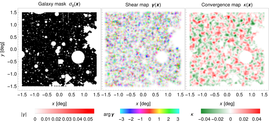
With the ellipticities simulated for all galaxies in a sub-field and a redshift bin, we can generate a $3\times 3\,\mathrm{{deg}^{2}}$ shear map on a $104\times 104$ square grid, and we add 12 pixels of padding on all four sides of the map to better maintain the lensing signal near the edge during smoothing (see below). The size of the full map is therefore $3.69\times 3.69\,\mathrm{{deg}^{2}}$ with a dimension of $128\times 128$, and the size of each pixel is $\Delta x=1.73\,\mathrm{arcmin}$.

In the HSC catalogue, there are regions without galaxies due to bright stars, and we need to find this field mask $\sigma_{\mathrm{mask}}(\boldsymbol{x})$ for each sub-field, which will be used in the generation of shear maps. Note that the field mask does not depend on the redshift bin, thus the number density of the galaxies is high enough for us to calculate the mask at a resolution of $0.87\,\mathrm{arcmin}$, i.e. on a $208\times 208$ grid for a $3\times 3\,\mathrm{{deg}^{2}}$ sub-field. The sub-fields have 10 to 15 galaxies per pixel on average among all pixels with at least one galaxy, and based on that, we consider the pixels with fewer than four galaxies to be covered by the mask ($\sigma_{\mathrm{mask}}(\boldsymbol{x})=1$). Then, the field masks are down-sampled by a factor of two to the resolution of shear maps, an example of which is shown in Figure 6.

The calculation of the shear maps follows the shear estimation procedure as in Appendix 3 of Mandelbaum et al. 2018a. The value of the pixel centred at $\boldsymbol{x}\equiv(x,y)$ is

The fields on the right-hand side are defined as

where $\phi$ is one of $\{e_{\mathrm{RMS}}^{2},m_{\mathrm{tot}},\boldsymbol{c},\boldsymbol{e}\}$, $N$ the number of galaxies in the sub-field and the redshift bin, $w_{i}$ the lensing weight of the $i^{\text{th}}$ galaxy in the catalogue, and $\boldsymbol{x}_{i}\in A(\boldsymbol{x})$ means that the $i^{\text{th}}$ galaxy is located in the pixel centred at $\boldsymbol{x}$. We further simplify the calculation by assuming $\langle\boldsymbol{c}\rangle=\langle\boldsymbol{e}\rangle=0$. Note that due to the second terms in Equation (16) and (17), the average values (e.g. shears and biases) are assigned to the masked region of the map so that $\phi(\boldsymbol{x})$ and $\boldsymbol{\gamma}(\boldsymbol{x})$ are well-defined on the entire map. When smoothing of the shear map is needed, a Gaussian kernel with standard deviation $\sigma_{\mathrm{G}}$ is applied to $\phi_{w}(\boldsymbol{x})$ and $w(\boldsymbol{x})$, e.g.

The process of shear map generation from the real HSC catalogue is identical to the that from the simulated catalogues. An example shear map from the real HSC data with smoothing is shown in Figure 6.

We use the Kaiser–Squires method (Kaiser & Squires 1993) to convert the shear maps from the previous step to convergence maps $\kappa(\boldsymbol{x})$. In Fourier space, the shear $\hat{\boldsymbol{\gamma}}(\boldsymbol{\ell})$ and the convergence $\hat{\kappa}(\boldsymbol{\ell})$ are related by

Again, the same conversion is applied to the real HSC shear maps. An example convergence map from the HSC data is shown in Figure 6. All of our cosmological analyses will be done convergence maps.

The lensing shear from the ray-tracing method in § III.2 reproduces the interaction between the light from the source galaxy and the foreground matter distribution and the intrinsic ellipticities of the galaxies are randomly assigned. But in the real Universe, there can be an intrinsic alignment (IA) between the galaxies through two mechanisms: (1) galaxies that are physically close to each other tend to have similar ellipticities (intrinsic-intrinsic, or II), and (2) a foreground galaxy is correlated with a local matter distribution that distorts a background galaxy in the orthogonal direction (gravitational-intrinsic, or GI). In this work, we adopt the non-linear alignment model (Hirata & Seljak 2004; Bridle & King 2007) which predicts the power spectrum of the IA signal to be

where

In Equation (22), $A_{\mathrm{IA}}$ denotes a free parameter that controls the amplitude of IA, $C_{1}=5\times 10^{-14}h^{-2}\mathrm{M}_{\odot}^{-1}\mathrm{Mpc}^{3}$ a normalising constant, $\bar{\rho}(z)$ the mean matter density of the universe at redshift $z$, $D(z)$ the linear growth factor, and $\bar{L}$ the weighted average luminosity of the source sample. Following Fluri et al. 2019 and Hildebrandt et al. 2017, we ignore the redshift and luminosity dependent terms by setting $\eta=\beta=0$.

A natural simple choice for the IA-induced convergence field is linked to the matter distribution. Specifically, we follow Fluri et al. 2019 and adopt

where $n_{\mathrm{g}}^{(b)}(z)$ denotes the number of galaxies per redshift in the bin $b$ normalised with $\int\mathrm{d}z\,n_{\mathrm{g}}^{(b)}(z)=1$, and $\delta(\boldsymbol{x},\chi)$ the density contrast. This IA estimation yields the correct IA power spectrum by construction and can be easily incorporated into our ray-tracing subroutine. We can trace $\kappa_{\mathrm{IA}}(\boldsymbol{x})$ along with $\boldsymbol{\gamma}_{\mathrm{IA}}(\boldsymbol{x})$ for each galaxy. We note that $\kappa_{\mathrm{IA}}$ and $\boldsymbol{\gamma}_{\mathrm{IA}}$ are linearly proportional to $A_{\mathrm{IA}}$, and thus we only need to trace them with $A_{\mathrm{IA}}=1$ to get $\tilde{\kappa}_{\mathrm{IA}}(\boldsymbol{x})$ and $\tilde{\boldsymbol{\gamma}}_{\mathrm{IA}}(\boldsymbol{x})$—results for any other $A_{\mathrm{IA}}$ can be inferred via

In our analyses where IA is included in the model, we modify the calculation of the simulated ellipticity in Equation (11) by doing the following replacement:

The shape of a galaxy when observed by a ground-based telescope is contaminated by effects like atmospheric disturbances and instrument characteristics. They can be modelled by a PSF, which modifies the shape of the source through convolution. A typical approach to remove the PSF from a galaxy shape involves two steps: (1) predict the shape of the PSF at the location of the galaxy using nearby stellar images, and (2) apply a PSF deconvolution algorithm, such as the re-Gaussianization method in the HSC pipeline. Nevertheless, both steps can still leave small residual PSF in the galaxy shapes: (1) the number density of stars is much smaller than that of galaxies, thus the variations of PSF on small angular scales can not be accurately predicted, and (2) the PSF deconvolution algorithm can have imperfections that leaks PSF shape into the deconvolved galaxy shape (Mandelbaum et al. 2018a). We follow Hikage et al. 2019 and Hamana et al. 2020 to model PSF residuals as a linear combination of these two effects:

where $\boldsymbol{\gamma}^{\mathrm{p}}=\boldsymbol{e}^{\mathrm{psf}}/2$ denotes the shear associated with the predicted PSF shape, and $\boldsymbol{\gamma}^{\mathrm{q}}=\boldsymbol{\gamma}^{\mathrm{p}}-\boldsymbol{\gamma}_{\mathrm{true}}^{\mathrm{p}}$ the difference between the predicted PSF shear and the untraceable true PSF shear.

As the small scale variations of PSFs is not recoverable, it is not possible to reproduce $\boldsymbol{\gamma}^{\mathrm{q}}$ fields that have identical characteristics to the real data. We therefore adopt an alternative approach where we model the the PSF residuals as Gaussian random fields, and they can be generated based on the auto- and cross-correlation functions between $\boldsymbol{\gamma}^{\mathrm{p}}$ and $\boldsymbol{\gamma}^{\mathrm{q}}$ measured by Hamana et al. 2020. We choose the correlation functions because they are measured at a higher angular scale resolution than the power spectra by Hikage et al. 2019. We fit analytical models to the correlation functions presented in Figure 20 of Hamana et al. 2020 and derive their power spectra counterparts ($C^{\mathrm{pp}}$, $C^{\mathrm{pq}}$, and $C^{\mathrm{qq}}$) by the Hankel transform

Visualisations of the correlation functions and power spectra are shown in Figure 7. The total PSF error power spectrum is a linear combination of the three components:

where the nuisance parameters $\alpha$ and $\beta$ have Gaussian priors derived from Figure 21 in Hamana et al. 2020 with all angular scales:

After the convergence maps are generated for a realisation (see Section III.7), we sample $\alpha_{\mathrm{psf}}$ and $\beta_{\mathrm{psf}}$ from their prior distributions and generate one PSF convergence map for each sub-field, which is added to the convergence maps for all redshift bins.

In addition to the CNN, we also perform analyses with cross power spectra and tomographic peak counts on the same set of convergence maps, so that we can fairly compare their qualities.

The cross power spectrum between the convergence maps of two redshift bins $j$ and $k$ ($1\leq j\leq k\leq 4$) is measured by:

where $i=1,\cdots,8$ denote the indices of the multipole bins, $\ell_{i}=10^{2.4+i/10}$ the boundaries of the bins, $N_{\mathrm{mode},i}$ the number of multipole modes in the $i^{\mathrm{th}}$ bin, $C^{jk}(\boldsymbol{\ell})$ the cross power spectrum at multipole $\boldsymbol{\ell}$. The multipole range of the measured cross power spectra is $316<\ell<1995$, comparable to that in Hikage et al. 2019. Across all ten pairs of the redshift bins, the cross power spectra of a tomographic convergence map produces a data vector with 80 numbers.

The peak counts of a convergence map in a redshift bin is defined to be the histogram of all peak values in the map, where a pixel is a peak if and only if its $\kappa$ value is greater than all eight of its neighbours. We smooth the maps by a Gaussian kernel with radius $\sigma_{\mathrm{G}}=2\,\mathrm{arcmin}$ to remove small scale fluctuations. By inspecting the convergence maps at the fiducial cosmology, we find the typical standard deviations of $\kappa$ across the maps are $\sigma_{\kappa}=0.015,0.016,0.019,0.025$ in the four redshift bins (low to high) respectively. Then number of peaks are counted in 20 equally-spaced $\kappa$ bins in the range of $-1\,\sigma_{\kappa}^{(b)}\leq\kappa\leq 4\,\sigma_{\kappa}^{(b)}$, with the width of each bin being $0.25\,\sigma_{\kappa}^{(b)}$ for the $b^{\text{th}}$ redshift bin.

First, we compare our simulation pipeline to the T17 mock simulations by constraining the cosmological parameters with the T17 mock catalogues generated in Section II.2. Specifically, we calculate the data vector for each mock catalogue realisation and use the average data vector as the target data vector in Equation (36).²² 2 A more rigorous comparison can be made by setting the target data vector to the data vector from each realisation and summarising the properties of the posterior distributions, instead of using a single averaged data vector. We show the posterior distributions in Figure 8, together with the constraints where the data vector is calculated with our own simulated catalogues at the fiducial cosmology. Here, we use the configurations mock and no-systematics, where the IAs, baryons, and other systematics are not included, because non of these are added to T17 mock catalogues. To make the contours easier to read, we plot $S_{8}$ instead of $\sigma_{8}$ in Figure 8 and hereafter.

We find that the posterior distribution from our fiducial catalogues and that from T17 simulations are very similar other than small translations. In terms of the marginal distributions of $S_{8}$, the median $S_{8}$ values from the T17 mock catalogues are lower than that from our fiducial cosmology by $3.5\times 10^{-3}$, $6.4\times 10^{-3}$, and $3.7\times 10^{-3}$ for the power spectrum, peak counts, and CNN respectively. In comparison, the actual $S_{8}$ difference from cosmological parameters of the simulations is $\Delta S_{8}=9.2\times 10^{-3}$—the discrepancy is very small relative to the statistical error of $S_{8}$. We conclude that our model prediction and parameter inference pipelines passed this validation step.

Additionally, we note that the contours from our fiducial catalogues (the solid contours in Figure 8) are in general not centred around $\Omega_{\mathrm{m}}=0.3$ and $S_{8}=0.8$. In particular for the power spectrum, the maximum likelihood is reached at $(\Omega_{\mathrm{m}}=0.290,S_{8}=0.786)$. The reason is that the determinant of the covariance matrix varies across the cosmological parameter space, which affects the posterior probability in the prefactor of Equation (35). This phenomenon is especially significant for the power spectrum because the determinant decreases by a factor of two when $S_{8}$ increases from 0.796 to 0.804 (a one percent increase).

References

- Abbott et al. (2016) Abbott, T., Abdalla, F., Allam, S., et al. 2016, Physical Review D, 94, 022001
- Abbott et al. (2022) Abbott, T., Aguena, M., Alarcon, A., et al. 2022, Physical Review D, 105, 023520
- Abruzzo & Haiman (2019) Abruzzo, M. W., & Haiman, Z. 2019, Monthly Notices of the Royal Astronomical Society, 486, 2730
- Aihara et al. (2018a) Aihara, H., Arimoto, N., Armstrong, R., et al. 2018a, Publications of the Astronomical Society of Japan, 70, S4
- Aihara et al. (2018b) Aihara, H., Armstrong, R., Bickerton, S., et al. 2018b, Publications of the Astronomical Society of Japan, 70, S8
- Alam et al. (2017) Alam, S., Ata, M., Bailey, S., et al. 2017, Monthly Notices of the Royal Astronomical Society, 470, 2617
- Anderson et al. (2014) Anderson, L., Aubourg, É., Bailey, S., et al. 2014, Monthly Notices of the Royal Astronomical Society, 441, 24
- Aricò et al. (2020) Aricò, G., Angulo, R. E., Hernández-Monteagudo, C., et al. 2020, Monthly Notices of the Royal Astronomical Society, 495, 4800
- Asgari et al. (2021) Asgari, M., Lin, C.-A., Joachimi, B., et al. 2021, Astronomy & Astrophysics, 645, A104
- Bartelmann & Schneider (2001) Bartelmann, M., & Schneider, P. 2001, Physics Reports, 340, 291
- Bernstein & Jarvis (2002) Bernstein, G., & Jarvis, M. 2002, The Astronomical Journal, 123, 583
- Bridle & King (2007) Bridle, S., & King, L. 2007, New Journal of Physics, 9, 444
- Coxeter & Coxeter (1989) Coxeter, H., & Coxeter, H. 1989, Introduction to Geometry, Wiley Classics Library (Wiley). https://books.google.com/books?id=c0ld-crynsIC
- Dietrich & Hartlap (2010) Dietrich, J. P., & Hartlap, J. 2010, MNRAS, 402, 1049, doi: 10.1111/j.1365-2966.2009.15948.x
- Dodelson & Zhang (2005) Dodelson, S., & Zhang, P. 2005, Physical Review D, 72, 083001
- Fang & Haiman (2007) Fang, W., & Haiman, Z. 2007, Physical Review D, 75, 043010
- Fluri et al. (2019) Fluri, J., Kacprzak, T., Lucchi, A., et al. 2019, Physical Review D, 100, 063514
- Fluri et al. (2022) —. 2022, Physical Review D, 105, 083518
- Fu et al. (2014) Fu, L., Kilbinger, M., Erben, T., et al. 2014, Monthly Notices of the Royal Astronomical Society, 441, 2725
- Gupta et al. (2018) Gupta, A., Matilla, J. M. Z., Hsu, D., & Haiman, Z. 2018, Physical Review D, 97, 103515
- Hahn & Abel (2011) Hahn, O., & Abel, T. 2011, Monthly Notices of the Royal Astronomical Society, 415, 2101
- Hamana et al. (2020) Hamana, T., Shirasaki, M., Miyazaki, S., et al. 2020, Publications of the Astronomical Society of Japan, 72, 16
- Hartlap et al. (2007) Hartlap, J., Simon, P., & Schneider, P. 2007, Astronomy & Astrophysics, 464, 399
- He et al. (2016) He, K., Zhang, X., Ren, S., & Sun, J. 2016, in Proceedings of the IEEE conference on computer vision and pattern recognition, 770–778
- Heymans et al. (2021) Heymans, C., Tröster, T., Asgari, M., et al. 2021, Astronomy & Astrophysics, 646, A140
- Hikage et al. (2019) Hikage, C., Oguri, M., Hamana, T., et al. 2019, Publications of the Astronomical Society of Japan, 71, 43
- Hilbert et al. (2009) Hilbert, S., Hartlap, J., White, S., & Schneider, P. 2009, Astronomy & Astrophysics, 499, 31
- Hildebrandt et al. (2017) Hildebrandt, H., Viola, M., Heymans, C., et al. 2017, Monthly Notices of the Royal Astronomical Society, 465, 1454
- Hinshaw et al. (2013) Hinshaw, G., Larson, D., Komatsu, E., et al. 2013, The Astrophysical Journal Supplement Series, 208, 19
- Hirata & Seljak (2004) Hirata, C. M., & Seljak, U. 2004, Physical Review D, 70, 063526
- Jain et al. (2000) Jain, B., Seljak, U., & White, S. 2000, The Astrophysical Journal, 530, 547
- Jain & Van Waerbeke (2000) Jain, B., & Van Waerbeke, L. 2000, The Astrophysical Journal, 530, L1
- Joudaki et al. (2016) Joudaki, S., Blake, C., Heymans, C., et al. 2016, Monthly Notices of the Royal Astronomical Society, stw2665
- Kaiser & Squires (1993) Kaiser, N., & Squires, G. 1993, The Astrophysical Journal, 404, 441
- Kilbinger (2015) Kilbinger, M. 2015, Reports on Progress in Physics, 78, 086901, doi: 10.1088/0034-4885/78/8/086901
- Kilbinger et al. (2009) Kilbinger, M., Benabed, K., Guy, J., et al. 2009, Astronomy & Astrophysics, 497, 677
- Kingma & Ba (2014) Kingma, D. P., & Ba, J. 2014, arXiv preprint arXiv:1412.6980
- Köhlinger et al. (2016) Köhlinger, F., Viola, M., Valkenburg, W., et al. 2016, Monthly Notices of the Royal Astronomical Society, 456, 1508
- Kratochvil et al. (2010) Kratochvil, J. M., Haiman, Z., & May, M. 2010, Physical Review D, 81, 043519
- Kratochvil et al. (2012) Kratochvil, J. M., Lim, E. A., Wang, S., et al. 2012, Physical Review D, 85, 103513
- Krizhevsky et al. (2012) Krizhevsky, A., Sutskever, I., & Hinton, G. E. 2012, Advances in neural information processing systems, 25, 1097
- Kuijken et al. (2015) Kuijken, K., Heymans, C., Hildebrandt, H., et al. 2015, Monthly Notices of the Royal Astronomical Society, 454, 3500
- Laigle et al. (2016) Laigle, C., McCracken, H. J., Ilbert, O., et al. 2016, The Astrophysical Journal Supplement Series, 224, 24
- Leauthaud et al. (2017) Leauthaud, A., Saito, S., Hilbert, S., et al. 2017, Monthly Notices of the Royal Astronomical Society, 467, 3024
- LeCun et al. (1998) LeCun, Y., Bottou, L., Bengio, Y., & Haffner, P. 1998, Proceedings of the IEEE, 86, 2278
- Lin & Kilbinger (2015) Lin, C.-A., & Kilbinger, M. 2015, Astronomy & Astrophysics, 583, A70
- Liu et al. (2015) Liu, J., Petri, A., Haiman, Z., et al. 2015, Physical Review D, 91, 063507
- Liu et al. (2022) Liu, X., Yuan, S., Pan, C., et al. 2022, Monthly Notices of the Royal Astronomical Society, doi: 10.1093/mnras/stac2971
- Lu & Haiman (2021) Lu, T., & Haiman, Z. 2021, Monthly Notices of the Royal Astronomical Society, 506, 3406, doi: 10.1093/mnras/stab1978
- Lu et al. (2022) Lu, T., Haiman, Z., & Zorrilla Matilla, J. M. 2022, Monthly Notices of the Royal Astronomical Society, 511, 1518
- Mandelbaum et al. (2018a) Mandelbaum, R., Miyatake, H., Hamana, T., et al. 2018a, Publications of the Astronomical Society of Japan, 70, S25
- Mandelbaum et al. (2018b) Mandelbaum, R., Lanusse, F., Leauthaud, A., et al. 2018b, Monthly Notices of the Royal Astronomical Society, 481, 3170
- Martinet et al. (2018) Martinet, N., Schneider, P., Hildebrandt, H., et al. 2018, Monthly Notices of the Royal Astronomical Society, 474, 712
- Munshi et al. (2011) Munshi, D., van Waerbeke, L., Smidt, J., & Coles, P. 2011, MNRAS, submitted, e-print arXiv:1103.1876. https://arxiv.org/abs/1103.1876
- Petri et al. (2013) Petri, A., Haiman, Z., Hui, L., May, M., & Kratochvil, J. M. 2013, Physical Review D, 88, 123002
- Petri et al. (2016) Petri, A., Haiman, Z., & May, M. 2016, Physical Review D, 93, 063524
- Petri et al. (2017) Petri, A., Haiman, Z., & May, M. 2017, Phys. Rev. D, 95, 123503, doi: 10.1103/PhysRevD.95.123503
- Planck Collaboration et al. (2020) Planck Collaboration, Aghanim, N., Akrami, Y., et al. 2020, A&A, 641, A6, doi: 10.1051/0004-6361/201833910
- Potter et al. (2017) Potter, D., Stadel, J., & Teyssier, R. 2017, Computational Astrophysics and Cosmology, 4, 1
- Redmon et al. (2016) Redmon, J., Divvala, S., Girshick, R., & Farhadi, A. 2016, in Proceedings of the IEEE conference on computer vision and pattern recognition, 779–788
- Refregier (2003) Refregier, A. 2003, Annual Review of Astronomy and Astrophysics, 41, 645
- Ren et al. (2015) Ren, S., He, K., Girshick, R., & Sun, J. 2015, Advances in neural information processing systems, 28, 91
- Ribli et al. (2019) Ribli, D., Pataki, B. Á., Zorrilla Matilla, J. M., et al. 2019, Monthly Notices of the Royal Astronomical Society, 490, 1843
- Schneider & Teyssier (2015) Schneider, A., & Teyssier, R. 2015, Journal of Cosmology and Astroparticle Physics, 2015, 049
- Shirasaki et al. (2019) Shirasaki, M., Hamana, T., Takada, M., Takahashi, R., & Miyatake, H. 2019, Monthly Notices of the Royal Astronomical Society, 486, 52
- Singh et al. (2015) Singh, S., Mandelbaum, R., & More, S. 2015, Monthly Notices of the Royal Astronomical Society, 450, 2195
- Sobol’ (1967) Sobol’, I. M. 1967, Zhurnal Vychislitel’noi Matematiki i Matematicheskoi Fiziki, 7, 784
- Takada & Jain (2003) Takada, M., & Jain, B. 2003, Monthly Notices of the Royal Astronomical Society, 344, 857
- Takada & Jain (2004) —. 2004, Monthly Notices of the Royal Astronomical Society, 348, 897
- Takahashi et al. (2017) Takahashi, R., Hamana, T., Shirasaki, M., et al. 2017, The Astrophysical Journal, 850, 24
- Takahashi et al. (2012) Takahashi, R., Sato, M., Nishimichi, T., Taruya, A., & Oguri, M. 2012, The Astrophysical Journal, 761, 152
- Tanaka et al. (2018) Tanaka, M., Coupon, J., Hsieh, B.-C., et al. 2018, Publications of the Astronomical Society of Japan, 70, S9
- Troxel et al. (2018) Troxel, M. A., MacCrann, N., Zuntz, J., et al. 2018, Physical Review D, 98, 043528
- Vafaei et al. (2010) Vafaei, S., Lu, T., van Waerbeke, L., et al. 2010, Astroparticle Physics, 32, 340