Risk-Averse MDPs under Reward Ambiguity
Abstract
We propose a distributionally robust return-risk model for Markov decision processes (MDPs) under risk and reward ambiguity. The proposed model optimizes the weighted average of mean and percentile performances, and it covers the distributionally robust MDPs and the distributionally robust chance-constrained MDPs (both under reward ambiguity) as special cases. By considering that the unknown reward distribution lies in a Wasserstein ambiguity set, we derive the tractable reformulation for our model. In particular, we show that that the return-risk model can also account for risk from uncertain transition kernel when one only seeks deterministic policies, and that a distributionally robust MDP under the percentile criterion can be reformulated as its nominal counterpart at an adjusted risk level. A scalable first-order algorithm is designed to solve large-scale problems, and we demonstrate the advantages of our proposed model and algorithm through numerical experiments.
haolin.ruan@my.cityu.edu.hk Department of Management Sciences, College of Business, City University of Hong Kong, Kowloon Tong, Hong Kong
zhi.chen@cityu.edu.hk School of Data Science, City University of Hong Kong, Kowloon Tong, Hong Kong
clint.ho@cityu.edu.hk ††affiliation: ††affiliation: ††affiliation: ††affiliation: ††affiliation: ††affiliation:
1 Introduction
Markov decision processes (MDPs) provide a powerful modeling framework for sequential decision-making problems and reinforcement learning in stochastic dynamic environments (Puterman 2014). Obtaining the model parameters of MDPs that perfectly reflect the environments, however, has always been a challenge in practice, as these parameters are estimated from limited data that are potentially contaminated (Mannor et al. 2007). Moreover, these parameters, such as transition kernel and reward function, are often time-dependent or even uncertain, but they are approximated as fixed values in an overly simplified setting (Mannor et al. 2016). Therefore, the output policies of MDPs are often disappointing in practice.
Robust MDPs address the aforementioned issues of parameter ambiguity, by allowing the unknown values of transition kernels and reward functions to lie in a given ambiguity set (Behzadian et al. 2021, Chen et al. 2019, Clement and Kroer 2021a, Delgado et al. 2016). Then, robust MDPs seek for policies that maximize the worst-case expected return over all transition kernels and reward functions in the ambiguity sets. By specifying ambiguity sets that contain the unknown transition kernels with high confidence, the optimal policies of robust MDPs are robust to parameter ambiguity (Iyengar 2005).
In this paper, we focus on the case where the reward function is ambiguous, which sometimes is referred to as imprecise-reward MDPs (Alizadeh et al. 2015, Regan and Boutilier 2010, Regan and Boutilier 2011a, Regan and Boutilier 2011b, Regan and Boutilier 2012). This particular setting is also closely related to imitation learning, which trains an agent to learn a certain behavior of an expert, while only some demonstrated trajectories of her is available (Chen et al. 2020, Ho and Ermon 2016, Osa et al. 2018, Rashidinejad et al. 2021). When applying inverse reinforcement learning approach to learn the reward function that completely represents the expert’s preference (Brown et al. 2020, Choi and Kim 2012, Ng et al. 2000), the yielded policies, which suffer from reward ambiguity, may perform poorly in practice.
To handle reward ambiguity, we utilize techniques from distributionally robust optimization (DRO) (Derman and Mannor 2020) and distributionally robust chance-constrained program (Chen et al. 2007, Postek et al. 2018), assuming that the true reward distribution resides in an ambiguity set. This approach does not require the reward function to be precisely specified. Instead, only the descriptions of common distribution information such as support, moments and shape in the ambiguity set are needed, which are often much easier to be obtained/estimated (Hanasusanto et al. 2015, Hanasusanto et al. 2017, Zymler et al. 2013). In this paper, we consider a Wasserstein ambiguity set for our distributionally robust models as in Abdullah et al. 2019, Calafiore and Ghaoui 2006, Xie 2021. Unlike phi-divergence ambiguity sets which may contain too extreme member distributions, the closeness between points in the support set is incorporated in Wasserstein sets, thus their member distributions may be more reasonable (Gao and Kleywegt 2022); on the other hand, Wasserstein sets are often a better choice than moment-based ambiguity sets when the number of samples is too small to obtain a reliable estimation on moments (Yang 2020). We choose Wasserstein sets for these reasons, although other types of ambiguity sets such as nested ambiguity sets (Xu and Mannor 2010, Xu and Mannor 2012) and the ambiguity sets based on Prohorov metric (Erdoğan and Iyengar 2006) are also considered in literature. For our distributionally robust chance-constrained MDPs, we will furthermore show its equivalence with the nominal counterparts with an adjusted risk level. To the best of our knowledge, this is the first result in MDPs that establishes the mutual transformation between distributional ambiguity and risk.
Our return-risk model (RR) is a risk-averse MDP model that not only takes into account reward ambiguity, but also considers both the average and risk of the return. MDPs that minimize the risk of the return instead of the expected cost are called risk-aware MDPs (also called risk-sensitive or risk-averse MDPs) (Ahmadi et al. 2021, Bäauerle and Rieder 2017, Carpin et al. 2016, Haskell and Jain 2015, Huang and Haskell 2017). In risk-aware optimization, the objective function is taken as a risk measure, such as value-at-risk (VaR) (Delage and Mannor 2007, Delage and Mannor 2010, Gilbert et al. 2017), conditional value-at-risk (CVaR) (Bäuerle and Ott 2011, Chow et al. 2017, Huang and Guo 2016) and other spectral risk measures (Bäuerle and Glauner 2021), and variants of expected utility (Bernard et al. 2022, Jaimungal et al. 2022, Pflug and Wozabal 2007).
Among these risk measures, VaR and CVaR are arguably the most popular ones and have attracted the attention of many researchers (Bäuerle and Ott 2011, Chow et al. 2017, Delage and Mannor 2007, Delage and Mannor 2010, Gilbert et al. 2017, Huang and Guo 2016). By using CVaR, one aims to give a precise depiction of the extreme tail of the distribution (of the uncertain rewards), while VaR does not reflect the extreme scenerios exceeding VaR. It is well-known that CVaR is a coherent risk measure, which can be efficiently optimized by convex optimization tools (Chen and Xie 2021); in contrast, VaR is a more challenging risk measure because it is not a coherent one.
One remarkable advantage of VaR is its stability of estimation (especially under fat-tailed reward distribution (Sarykalin et al. 2008)), which is particularly important under data-driven settings where the number of samples are limited and decision makers evaluate models based on their out-of-sample performances (Bertsimas and Thiele 2006, van de Berg et al. 2022, Zheng et al. 2016). To demonstrate, we provide an example where we consider a one-step MDP with only 1 state and 2 actions and (Sutton and Barto 2018). In this one-step MDP, the decision maker only makes one decision in each episode, and she aims to maximize her VaR/CVaR of rewards for these episodes. We consider uncertain rewards and where is a Student’s -distribution and we vary its degree of freedom . We set the shift ratios , and for testing the estimation accuracy w.r.t. VaR (resp., CVaR) (where we choose the risk threshold ), we set the shift quantity as (resp., ), where both risk measures can be efficiently calculated (see Appendix B for more details). We evaluate the decision maker’s accuracy rate as the proportion of testing samples where she has chosen the action with a higher VaR/CVaR of rewards (i.e., action ); for each pair of accuracy rate and shift ratio, following Yamai et al. 2002, 1000 random reward samples for each state-action pair are available for the decision maker, and we test her accuracy rate based on 10000 testing samples.
As illustrated in Figure 1, the accuracy rate increases with the shift ratio . As decreases, becomes more fat-tailed, and the accuracy rate of VaR is remarkably higher than that of CVaR, which indicates that the statistical inference on VaR would be more accurate than on CVaR. Therefore, VaR may be a more preferable choice when only small sample sets are available.
Our return-risk model is motivated by the soft-robust criterion/model, which optimizes a convex combination of the mean and a robust performance in the optimization literature (Ben-Tal et al. 2010). MDPs with soft-robustness are also popular in recent years, where decision makers aim to maximize a weighted average of the mean and percentile performances (Brown et al. 2020, Lobo et al. 2020). Unlike these existing soft-robust MDPs, however, the proposed return-risk model is fundamentally different in two aspects: first, these existing soft-robust models have no consideration for reward ambiguity, while we utilize distributionally robustness to account for reward ambiguity, by which we can hedge against the most adversarial realization of the distribution of rewards (within the ambiguity set), thus our model is more robust to reward uncertainty (Chen et al. 2019, Xu and Mannor 2010); second, we choose VaR as the risk measure which has a direct interpretation to percentile performances, and, as illustrated above, tends to be more advantageous in data-driven optimization.
Our work concentrates on model-based setting, where our proposed models are motivated by the classical (dual formulation of) nominal MDPs (Puterman 2014) and the chance-constrained MDPs (Delage and Mannor 2010). It is worth noting that, beyond model-based setting, there are other inspiring and innovative researches on robust reinforcement learning, such as robust TDC algorithms and robust Q-learning (Roy et al. 2017, Wang and Zou 2021), robust policy gradient (Wang and Zou 2022), least squares policy iteration (Lagoudakis and Parr 2003) and sample complexity analysis (Panaganti and Kalathil 2022). Note that, though model-free reinforcement learning can be used to learn satisfactory policies for complex environment, the requirement of large amounts of interaction (with environment) may render the learning process slow (Kaiser et al. 2019), while high sample efficiency is one strong advantage of model-based learning (Sutton and Barto 2018). We also note that MDPs with transition kernel ambiguity is another active research line where distributionally robustness is widely employed (Clement and Kroer 2021b, Shapiro 2016, Shapiro 2021, Xu and Mannor 2012).
We may summarize our contributions as follows (and we also compare our contributions to those of related works in Table 2 in Appendix I).
(i) We show that the distributionally robust model of optimizing expected rewards can be reformulated as a convex conic program, which is equivalent to the nominal MDP with a convex regularization in the objective function.
(ii) For distributionally robust chance-constrained MDPs (DCC), we show that it can be reformulated as nominal chance-constrained MDPs at adjusted risk levels. This observation bridges the gap between risk and parameter ambiguity.
(iii) Combining the proposed models in (i) and (ii), we propose the return-risk MDP that maximizes the weighted average of the expectation and VaR of reward (both under distributionally robustness to reward uncertainty), which is flexible and can perform well under the criteria of mean and percentile returns.
(iv) When only considering deterministic policies, we show that our return-risk model can also account for risk from uncertain transition kernel, and we derive its equivalent reformulation as a mixed-integer second-order cone program (MISOCP).
(v) To solve the proposed return-risk model, we design a first-order method that is more scalable than the MOSEK solver, thus is faster with large-size problems.
(vi) In the simulation and empirical experiments, we adopt a data-driven setting, where the decision maker aims at maximizing the expectation and VaR of the random reward. We compare the performances of distributionally robust MDPs (DRMDPs), DCC, RR, robust MDPs (RMDPs) (Delage and Mannor 2010) and BROIL (Brown et al. 2020), and results show that the third one performs the best under both expectation and different VaR’s (with risk thresholds and ), which showcases its advantages and adjustability to the decision makers’ changeable preferences between return and risk.
The remainder of this paper is organized as follows. We introduce the background in Section 2. In Sections 3 and 4, we study DRMDPs as well as the DCC model, respectively, and we derive their tractable reformulations. Combining these proposed models, we propose the RR model in Section 5. The designed first-order algorithm for the RR model is detailed in Section 6. We compare the performances of DRMDP, DCC, RR, RMDP and BROIL, and demonstrate the advantage of our proposed algorithm in Section 7. Conclusion is drawn in Section 8.
2 Background
We consider an infinite-horizon MDP with a finite state space and a finite action space . Let be the transition probability kernel such that is denoted to be the transition probability of transiting to state when action is chosen in state ; thus, is the transition probability distribution for every . Given the state-action pair , an agent will receive an expected reward . To simplify our notation, we denote the reward function as a vector .
We seek for the optimal stationary randomized policy with for all , where an action will be taken in state with probability . A nominal MDP that maximizes the expected reward can be formulated (Puterman 2014) as
| (1) |
where the feasible set is given by Here the coefficient matrices with all-ones vectors and with for all . For each , we denote the subvector of as ; its component can be interpreted as the total discounted probability one occupying state and choosing action when applying the policy (Puterman 2014)11 1 By Puterman 2014, any admits such interpretation, thus we can retrieve our policies of all the proposed models in this paper in this way.. We have a discount factor and the initial distribution of the initial states. Problem (1) is a linear program that can be efficiently solved by simplex method and interior-point method (Nocedal and Wright 2006). One can also compute the optimal policy efficiently by applying value iteration or policy iteration to solve the associated Bellman equation of this problem (Bertsekas and Tsitsiklis 1995, Puterman 2014).
The nominal MDP (1) does not account for uncertainty in either rewards or transition kernel. To account for reward uncertainty, Delage and Mannor 2010 assume that the random reward vector follows a known Gaussian distribution and propose a chance-constrained MDP model as follows:
| (2) |
In fact, the above chance-constrained model maximizes the VaR (at the risk level ) of the reward with respect to the distribution . Since is assumed Gaussian, by theorem 10.4.1 in Prékopa 2013, one can reformulate problem (2) as a second-order cone program as follows:
where is the inverse of the cumulative density function of the Gaussian distribution and is the covariance matrix of . Second-order cone programs allow efficient solutions by state-of-the-art commercial solvers such as CPLEX, Gurobi and MOSEK (see, e.g., Ben-Tal and Nemirovski 2001). Despite its tractability, the chance-constrained MDP (2) requires the precise underlying reward distribution as input. Moreover, the above reformulation does not hold for generic distribution .
3 Distributionally Robust MDPs
In many real-world situations, the true distribution of the uncertain reward is hard (if not impossible) to obtain. Instead, we may have some firm knowledge, such as moments and shape about it. As one of the most efficacious treatments for such situations, the DRO approach models uncertainty as a random variable governed by an unknown probability distribution residing in an ambiguity set. Facing distributional ambiguity, a decision maker seeks for solutions that hedge against the most adversarial distribution from within the ambiguity set. To be specific, in our context, we assume that the true distribution of the uncertain reward resides in a Wasserstein ball of radius around some reference distribution :
| (3) |
Here is the set of all probability distributions on , and the Wasserstein distance between two distributions and , equipped with a general norm in , is given by where is the set of all joint distributions with marginal distributions and that govern and , respectively.
The random parameter in the nominal MDP (1) is the expectation of reward, which in practice, is often estimated by the average of historical samples. However, when the sample size is small, such a sample average is not close to the expectation but rather, is known to be optimistically biased (see, e.g., Smith and Winkler 2006). Hence, the nominal MDP (1) based on samples may yield an unsatisfactory policy that does not perform well out-of-sample. For this reason, a possible alternative is to maximize instead the worst-case expected reward as in the following distributionally robust MDP:
| (4) |
The following proposition offers an equivalent conic program for (4).
Proposition 3.1
The distributionally robust MDP (4) can be reformulated a conic program
It is not hard to observe that the distributionally robust MDPs can be viewed as a convex regularization of the nominal MDP (4) under the reference distribution . In particular, the convex regularizing term in the distributionally robust MDP is , which is sized by the Wasserstein radius . Interestingly, we have also found that an (distributionally) optimistic MDP can be reformulated as a reverse conic program with a (concave) regularization term . We relegate this result to Appendix D.
We remark that, problem (4) is indeed a special case of the robust optimization problem considered in Jaimungal et al. 2022, where we consider the expected utility framework. Compared to the policy gradient methods provided in Jaimungal et al. 2022 where convergence is not established, we have derived its equivalent reformulation as a tractable conic program which can be efficiently solved by state-of-the-art commercial solvers such as Gurobi, Mosek and CPLEX, and can also be seamlessly incorporated in the tractable reformulation of our proposed return-risk model in Section 5.
4 Distributionally Robust Chance-Constrained MDPs
In this section, we turn from optimizing the expectation of reward to its tailed performance, by exploring chance-constrained MDPs. In particular, we still consider Wasserstein ambiguity sets (3) to account for distributional ambiguity, meanwhile specifying the reference distribution and the norm in the definition of the Wasserstein distance.


For the former, we focus on an elliptical reference distribution = 22 2 Note that results in Section 3 hold for a general reference distribution. throughout this section, whose probability density distribution is given by where is a positive normalization scalar, is a mean vector, is a positive definite matrix and is a generating function. We emphasize that this assumption on is mild as this is only the center of the ambiguity set. In particular, our proposed distributionally robust chance-constrained MDPs can account for all types of distributions (as long as they are inside the ambiguity set) and they are not restricted to be all elliptical. As we shall see, such specifications lead to tractable reformulation of our proposed models. Preliminaries on elliptical distributions are relegated to Appendix C.
For the latter, we adopt the Mahalanobis norm associated with the positive definite matrix , captured by . Note that the dual norm of a Mahalanobis norm is another Mahalanobis norm that is defined by the inverse matrix .
In a distributionally robust chance-constrained MDP, we hope that even in the worst-case, with a high confidence the reward is no less than a lower bound, and we aim at maximizing such a lower bound by solving
| (5) |
Quite notably, the worst-case chance constraint in the pessimistic chance-constrained MDP (5) is equivalent to a nominal chance constraint in (2) with a higher risky level.
Lemma 4.1
Suppose in the Wasserstein ambiguity set (3), the reference distribution is an elliptical distribution and the Wasserstein distance is equipped with a Mahalanobis norm associated with the positive definite matrix . The distributionally robust chance constraint
| (6) |
is satisfiable if and only if where with that can be computed via bisection method which searches for the smallest that satisfies
Equipped with Lemma 4.1, it then turns out that the distributionally robust chance-constrained MDP (5) is equivalent to a nominal chance-constrained MDP (2) at a higher risky level. Consequently, the distributionally robust chance-constrained MDP (5) can be reformulated into a conic program, or more precisely, a second-order cone program owing to our choice of the Mahalanobis norm.
Proposition 4.2
Suppose in the Wasserstein ambiguity set (3), the reference distribution is an elliptical distribution and the Wasserstein distance is equipped with a Mahalanobis norm associated with the positive definite matrix . If the risk threshold satisfies , then the distributionally robust chance-constrained MDP (5) is equivalent to the second-order cone program
where with being the smallest that satisfies
Similar to the distributionally robust MDPs in Section 3, the distributionally robust chance-constrained MDPs also admit an optimistic counterpart, which is equivalent to the nominal chance-constrained MDPs with a larger risk threshold. We relegate this result to Appendix E.
To conclude this section, we present in Figure 2 the relations between and . Indeed, for any fixed , there is a one-to-one correspondence between the risk threshold and the Wasserstein radius . Following from this fact, for the chance-constrained model in our numerical experiments (Section 7), we only calibrate the risk threshold rather than the Wasserstein radius.
5 Return-Risk MDP
For rational decision makers, two types of rewards are their chief concerns: the average and the worst-case rewards. However, the risk-averse models often can not achieve decent average return on which the model put no emphasis (Carpin et al. 2016, Delage and Mannor 2010, Jiang and Powell 2018). To take both concerns into considerations, we leverage the established DRMDPs and DCC model in Sections 3 and 4 as ingredients and propose the return-risk MDP that maximizes the weighted average of the worst-case expectation and VaR of reward as follows:
| (7) |
Here the Wasserstein ball is assumed equipped with a general reference distribution and an -norm in the definition of the Wasserstein distance, while an elliptical reference distribution and a Mahalanobis norm associated with the positive definite matrix are assumed for . It is not hard to see that the return-risk MDP (7) takes the distributionally robust MDP (4) and the distributionally robust chance-constrained MDP (5) in as special cases by varying , and . Furthermore, by choosing a fractional , the return-risk model enables one to tailor a balance between risk and return. Proposition 5.1 below provides an equivalent second-order cone program for the return-risk MDP (7) under these assumptions.
Proposition 5.1
Suppose in (7) the Wasserstein ball (resp., ) is equipped with a general distribution (resp., an elliptical reference distribution ) and the norms in the definitions of the Wasserstein distances of and are an -norm and the Mahalanobis norm associated with , respectively. Assume that the risk threshold satisfies , then the return-risk MDP (7) is equivalent to a second-order cone program
| (8) |
where with being the smallest that satisfies and it could be computed via bisection method.
5.1 Risk-Awareness for Uncertain Transition Kernel
By adopting the static soft-robust framework in Lobo et al. 2020, one can indeed also account for the uncertainty in transition kernel in our return-risk model. As in Lobo et al. 2020, suppose we have finite samples of transition kernel with weights that are generated by MCMC (see, e.g., Kruschke 2010). Our proposed model is then as follows:
| (9) |
Here the objective function in (9) is again soft-robust against the uncertainty (in transition kernel), with the weight as the controller for the robustness and is the risk threshold (w.r.t. the uncertain transition kernel). The weighted empirical distribution and the function
represents the optimal value of the return-risk model with the additional constraint that the optimal policy should be the input and with as the coefficient matrix corresponding to the input transition kernel .
Quite notably, when focusing on deterministic policies, one can reformulate (9) as an MISOCP.
Proposition 5.2
We remark that, though deterministic policies seem to be restricted compared to the randomized ones, they actually are more favored under some situations; for example, they may be a more suitable choice in some medical domains where randomized policies are unworkable for practical and philosophical reasons (Rosen et al. 2006). Also, randomized policies may be difficult to be evaluated after they have been deployed and may have poor reproducibility (Lobo et al. 2020).
6 First-Order Method
In this section, we introduce an efficient first-order algorithm to solve the equivalent formulation (8) of our return-risk model. Our algorithm is based on an alternating direction linearized proximal method of multipliers (AD-LPMM) algorithm (Beck 2017, Shefi and Teboulle 2014), which is a variant of the alternating direction method of multiplier (ADMM) algorithm and also has a convergence rate of (here is the number of iterations) proved by Beck 2017. The proposed splitting allows efficient update of variables in AD-LPMM (where the solutions are analytical or can be retrieved by an efficient bisection method).
For the primal update of the ADMM algorithm, one needs to solve minimization problems with a quadratic term involved (in its objective function); in AD-LPMM, this quadratic term can be linearized by adding a proximity term to the objective function, which could render the primal update much easier. To implement our AD-LPMM algorithm, first we will introduce auxiliary variables and rewrite (8) (as a minimization problem) as follows:
| (10) |
where, in the spirit of AD-LPMM, we can split the decision variables into two groups and update them separately. The augmented Lagrangian function of (10) is:
Based on our splitting method, we will update the two groups of variables and separately. For the update of , we define two primal update operators
and while for the update of (i.e., the second group of variables), we define
where and (equipped with a positive semi-definite matrix ) is a weighted vector norm such that . As we shall see in Section 6.3, the update of is fast (where an analytical solution is available) with the proximity term added. Note that when , the update in AD-LPMM degenerates to an ADMM’s one.
We now introduce our AD-LPMM in Algorithm 1. Basically, the most time-consuming computations lie in the primal update phase, where the updates are carried out by solving a minimization problem with other variables fixed at values after their last updates. As shall be detailed soon, owing to our variable splitting method, the primal updates are also quite fast, where analytical solutions or solutions obtained by bisection are available. Here we choose a stepsize that is increasing in every iteration (with a growth rate ), which in practice accelerates the convergence.
while do
step 5: ;
step 6: ;
// Increase stepsize
step 8: ;
end while
6.1 Subproblem in Step 1: Proximal Mapping and Projection
To solve , first we would utilize the technique of proximal mapping and establish the following equivalences:
| (11) |
where is the proximal mapping operator and
| (12) |
is the operator of projection on the unit ball Here, the first equality in (11) holds by the definition of the proximal mapping operator, and the second equality follows from,e.g., example in Beck 2017. Indeed, problem (12) allows an efficient solution obtained by a bisection method to locate its optimal dual solution (after which the optimal primal solution can be retrieved immediately), where the upper bound of the bisection is provided in Lemma A.1 relegated to Appendix A.4. The time complexity of the solution process (11), as well as the pseudocode for the bisection method, are provided in the following proposition.
Proposition 6.1
Problem can be solved in time , where is the desired precision of the bisection method.
6.2 Subproblem is Step 2: Componentwise Update
Problem can be decomposed into single-variable quadratic programming problems, each allowing an analytical solution. We summarize the time complexity and details in the following proposition.
Proposition 6.2
Problem can be solved in time .
6.3 Subproblem in Step 3: Linearization and Proximal Mapping
Compared to the update in ADMM, in our AD-LPMM, a proximity term is added to the objective function of the update in step . By choosing as mentioned in Section 6, we can linearize all the quadratic terms in , thus the solution can be obtained analytically by the technique of proximal mapping (meanwhile assuring the positive semi-definiteness of in every iteration of Algorithm 1). This solution process, as well as its time complexity, is provided in the following proposition.
Proposition 6.3
Problem can be solved in time .
7 Numerical Experiments
In this section, we conduct two numerical experiments to compare the performances of DRMDPs (4), CC (2)33 3 As we demonstrated in Section 4, a DCC is equivalent to a nominal chance-constrained one with an adjusted risk level, thus here we simply choose the latter as the benchmark., RR (7), RMDPs (Delage and Mannor 2010) and BROIL (Brown et al. 2020) (please see Appendices F and G for more details for the last two models). In both experiments, we train our reward functions with different sample sizes (100,200,300,400,500). For each sample size, performance of each model is evaluated for 100 times. The performance of each model is evaluated by expectation and VaR with risk thresholds . Cross validations are conducted for parameter selection (please see Appendix H.1 for details).
In Section 7.1, we conduct a simulation study where MDPs are generated randomly as in Regan and Boutilier 2012; In Section 7.2, we study a machine replacement problem introduced in Delage and Mannor 2010. As implied in our proofs, in this section, the Wasserstein ambiguity set of DRMDPs (4) will be equipped with a general reference distribution and an -norm for the Wasserstein distance; as for RR (7), we use a general reference distribution and an -norm in the definition of the Wasserstein distance for the Wasserstein ambiguity set , while for , we use an elliptical reference distribution and the Mahalanobis norm associated with the positive definite matrix for the Wasserstein distance. All optimization problems are solved by MOSEK on a GHz processor with GB memory.
7.1 Simulation Study
In this experiment, we follow the experiment setup in Regan and Boutilier 2012 where the number of reachable next-states and the transition kernel are randomly generated (both of which are known to decision makers). More details of the experiment setting are relegated to Appendix H.2.
As illustrated in Figures 5 and 7 (where the latter for VaR with is relegated to Appendix H.4), when the decision maker aims to optimize her tailed performances, CC is a preferable choice compared to DRMDPs; on the contrary, when pursuing optimizing the average return, DRMDPs perform much better than CC. Observe that the RR model, which includes both DRMDPs and the DCC model as special cases, remains as the best model under all criteria. In particular, one can observe that, RR achieves higher percentile returns than BROIL (that is a model without robustness), which demonstrates the benefits of distributionally robustness and the advantage of the risk measure VaR for percentile performance optimization. As expected, RMDPs end up yielding over-conservative policies; as a result, it performs poorly in most instances under all criteria.
7.2 Machine Replacement Problem
In this experiment, we follow the experiment setup in Delage and Mannor 2010 and consider the case where a factory holds an extensive amount of machines, each of which is subject to the same underlying MDP (more details of the experiment setting can be found in Appendix H.2). Our setting is similar to Delage and Mannor 2010 except for the follows: we use a data-driven setting as described above, and we evaluate our (policies of) models by looking at the various performance measures as in Section 7.1.
We report the overall performances of the five models in Figures 4 and 8 (where the latter for VaR with is relegated to Appendix H.5). Similar to the previous experiment, RR always performs better than or equal to the best model between CC and DRMDPs, and it provides the best performance under all criteria, which again manifest the merit of taking both the expected and worst-case performances into consideration and distributionally robustness.
7.3 Computation Times of Different Algorithms
| S=A | Runtimes | Relative gaps | |
|---|---|---|---|
| MOSEK | AD-LPMM | ||
| 40 | 0.60 | 2.79 | 0.1 |
| 70 | 5.58 | 4.81 | 0.1 |
| 100 | 25.50 | 19.98 | 0.2 |
| 130 | 93.54 | 66.17 | 0.1 |
| 160 | 444.06 | 168.34 | 0.4 |
In this section, we compare the computation times of our AD-LPMM algorithm with the state-of-the-art solver MOSEK. Table 1 reports the runtimes of the the AD-LPMM and MOSEK when solving problem (8) at different problem sizes. Results indicate that, though our AD-LPMM is slower than the MOSEK solver when problem size is small, it showcases its strong scalability and become much faster than MOSEK with large-size problems (while always maintaining high solution quality), where the advantage is more notable when the problem scales up.
8 Conclusion
We consider risk-aware MDPs with ambiguous reward functions and propose the return-risk model, which is versatile and can optimize any weighted combination of the average and quantile performances of a policy. This model generalizes and combines the advantage of distributionally robust MDPs and distributionally robust chance-constrained MDPs, thus is powerful in both average and percentile performances optimization. In particular, risk from uncertain transition kernel can also be captured by the return-risk model when output policies are deterministic. Tractable reformulations are provided for all our proposed models, and
Algorithm 1
we design an AD-LPMM algorithm for the return-risk model, which is well scalable and faster than the MOSEK solver with large-scale problems. Experimental results showcase the versatility of the return-risk model as well as
Algorithm 2
the scalability of the algorithm.
In the future, we believe that it would be important to explore more efficient methods for obtaining solution of RR, where function approximation and policy gradient (Sutton and Barto 2018) are possible choices to achieve this.
References
- Abdullah et al. (2019) Abdullah, Mohammed Amin, Hang Ren, Haitham Bou Ammar, Vladimir Milenkovic, Rui Luo, Mingtian Zhang, Jun Wang. 2019. Wasserstein robust reinforcement learning. arXiv preprint arXiv:1907.13196 .
- Ahmadi et al. (2021) Ahmadi, Mohamadreza, Ugo Rosolia, Michel Ingham, Richard Murray, Aaron Ames. 2021. Constrained risk-averse Markov decision processes. The 35th AAAI Conference on Artificial Intelligence (AAAI-21).
- Alizadeh et al. (2015) Alizadeh, Pegah, Yann Chevaleyre, Jean-Daniel Zucker. 2015. Approximate regret based elicitation in Markov decision process. The 2015 IEEE RIVF International Conference on Computing & Communication Technologies-Research, Innovation, and Vision for Future (RIVF). IEEE, 47–52.
- Bäauerle and Rieder (2017) Bäauerle, Nicole, Ulrich Rieder. 2017. Partially observable risk-sensitive Markov decision processes. Mathematics of Operations Research 42(4) 1180–1196.
- Bäuerle and Glauner (2021) Bäuerle, Nicole, Alexander Glauner. 2021. Minimizing spectral risk measures applied to Markov decision processes. Mathematical Methods of Operations Research 94(1) 35–69.
- Bäuerle and Ott (2011) Bäuerle, Nicole, Jonathan Ott. 2011. Markov decision processes with average-value-at-risk criteria. Mathematical Methods of Operations Research 74(3) 361–379.
- Beck (2017) Beck, Amir. 2017. First-order methods in optimization. SIAM.
- Behzadian et al. (2021) Behzadian, Bahram, Reazul Russel, Marek Petrik, Chin Pang Ho. 2021. Optimizing percentile criterion using robust MDPs. International Conference on Artificial Intelligence and Statistics 1009–1017.
- Ben-Tal et al. (2010) Ben-Tal, Aharon, Dimitris Bertsimas, David B Brown. 2010. A soft robust model for optimization under ambiguity. Operations research 58(4-part-2) 1220–1234.
- Ben-Tal and Nemirovski (2001) Ben-Tal, Aharon, Arkadi Nemirovski. 2001. Lectures on modern convex optimization: analysis, algorithms, and engineering applications. SIAM.
- Bernard et al. (2022) Bernard, Carole, Silvana M Pesenti, Steven Vanduffel. 2022. Robust distortion risk measures. arXiv preprint arXiv:2205.08850 .
- Bertsekas and Tsitsiklis (1995) Bertsekas, Dimitri, John Tsitsiklis. 1995. Neuro-dynamic programming: an overview. Proceedings of 1995 34th IEEE Conference on Decision and Control, vol. 1. IEEE, 560–564.
- Bertsimas and Thiele (2006) Bertsimas, Dimitris, Aurélie Thiele. 2006. Robust and data-driven optimization: modern decision making under uncertainty. Models, methods, and applications for innovative decision making. INFORMS, 95–122.
- Blanchet and Murthy (2019) Blanchet, Jose, Karthyek Murthy. 2019. Quantifying distributional model risk via optimal transport. Mathematics of Operations Research 44(2) 565–600.
- Brown et al. (2020) Brown, Daniel, Scott Niekum, Marek Petrik. 2020. Bayesian robust optimization for imitation learning. Advances in Neural Information Processing Systems 33 2479–2491.
- Calafiore and Ghaoui (2006) Calafiore, Carlo, L El Ghaoui. 2006. On distributionally robust chance-constrained linear programs. Journal of Optimization Theory and Applications 130(1) 1–22.
- Carpin et al. (2016) Carpin, Stefano, Yin-Lam Chow, Marco Pavone. 2016. Risk aversion in finite Markov decision processes using total cost criteria and average value at risk. 2016 IEEE International Conference on Robotics and Automation (ICRA). IEEE, 335–342.
- Chen et al. (2007) Chen, Xin, Melvyn Sim, Peng Sun. 2007. A robust optimization perspective on stochastic programming. Operations Research 55(6) 1058–1071.
- Chen et al. (2020) Chen, Xinyue, Zijian Zhou, Zheng Wang, Che Wang, Yanqiu Wu, Keith Ross. 2020. Bail: Best-action imitation learning for batch deep reinforcement learning. Advances in Neural Information Processing Systems 33 18353–18363.
- Chen et al. (2018) Chen, Zhi, Daniel Kuhn, Wolfram Wiesemann. 2018. Data-driven chance constrained programs over Wasserstein balls. arXiv preprint arXiv:1809.00210 .
- Chen et al. (2019) Chen, Zhi, Melvyn Sim, Huan Xu. 2019. Distributionally robust optimization with infinitely constrained ambiguity sets. Operations Research 67(5) 1328–1344.
- Chen and Xie (2021) Chen, Zhi, Weijun Xie. 2021. Sharing the value-at-risk under distributional ambiguity. Mathematical Finance 31(1) 531–559.
- Choi and Kim (2012) Choi, Jaedeug, Kee-Eung Kim. 2012. Nonparametric Bayesian inverse reinforcement learning for multiple reward functions. Advances in Neural Information Processing Systems 25.
- Chow et al. (2017) Chow, Yinlam, Mohammad Ghavamzadeh, Lucas Janson, Marco Pavone. 2017. Risk-constrained reinforcement learning with percentile risk criteria. The Journal of Machine Learning Research 18(1) 6070–6120.
- Clement and Kroer (2021a) Clement, Julien, Christian Kroer. 2021a. First-order methods for Wasserstein distributionally robust MDP. International Conference on Machine Learning. PMLR, 2010–2019.
- Clement and Kroer (2021b) Clement, Julien Grand, Christian Kroer. 2021b. First-order methods for wasserstein distributionally robust mdp. International Conference on Machine Learning. PMLR, 2010–2019.
- Delage and Mannor (2007) Delage, Erick, Shie Mannor. 2007. Percentile optimization in uncertain Markov decision processes with application to efficient exploration. Proceedings of the 24th International Conference on Machine Learning. PMLR, 225–232.
- Delage and Mannor (2010) Delage, Erick, Shie Mannor. 2010. Percentile optimization for Markov decision processes with parameter uncertainty. Operations Research 58(1) 203–213.
- Delgado et al. (2016) Delgado, Karina, Leliane De Barros, Daniel Dias, Scott Sanner. 2016. Real-time dynamic programming for Markov decision processes with imprecise probabilities. Artificial Intelligence 230 192–223.
- Derman and Mannor (2020) Derman, Esther, Shie Mannor. 2020. Distributional robustness and regularization in reinforcement learning. arXiv preprint arXiv:2003.02894 .
- Erdoğan and Iyengar (2006) Erdoğan, Emre, Garud Iyengar. 2006. Ambiguous chance constrained problems and robust optimization. Mathematical Programming 107(1) 37–61.
- Gao and Kleywegt (2016) Gao, Rui, Anton Kleywegt. 2016. Distributionally robust stochastic optimization with Wasserstein distance. arXiv preprint arXiv:1604.02199 .
- Gao and Kleywegt (2022) Gao, Rui, Anton Kleywegt. 2022. Distributionally robust stochastic optimization with Wasserstein distance. Mathematics of Operations Research .
- Gilbert et al. (2017) Gilbert, Hugo, Paul Weng, Yan Xu. 2017. Optimizing quantiles in preference-based Markov decision processes. Proceedings of the AAAI Conference on Artificial Intelligence, vol. 31.
- Hanasusanto et al. (2015) Hanasusanto, Grani, Vladimir Roitch, Daniel Kuhn, Wolfram Wiesemann. 2015. A distributionally robust perspective on uncertainty quantification and chance constrained programming. Mathematical Programming 151(1) 35–62.
- Hanasusanto et al. (2017) Hanasusanto, Grani, Vladimir Roitch, Daniel Kuhn, Wolfram Wiesemann. 2017. Ambiguous joint chance constraints under mean and dispersion information. Operations Research 65(3) 751–767.
- Haskell and Jain (2015) Haskell, William, Rahul Jain. 2015. A convex analytic approach to risk-aware Markov decision processes. SIAM Journal on Control and Optimization 53(3) 1569–1598.
- Ho and Ermon (2016) Ho, Jonathan, Stefano Ermon. 2016. Generative adversarial imitation learning. Advances in neural information processing systems 29.
- Hogg and Craig (1995) Hogg, Robert V, Allen T Craig. 1995. Introduction to mathematical statistics.(5”” edition). Englewood Hills, New Jersey .
- Huang and Haskell (2017) Huang, Wenjie, William Haskell. 2017. Risk-aware q-learning for Markov decision processes. 2017 IEEE 56th Annual Conference on Decision and Control (CDC). IEEE, 4928–4933.
- Huang and Guo (2016) Huang, Yonghui, Xianping Guo. 2016. Minimum average value-at-risk for finite horizon semi-Markov decision processes in continuous time. SIAM Journal on Optimization 26(1) 1–28.
- Iyengar (2005) Iyengar, Garud. 2005. Robust dynamic programming. Mathematics of Operations Research 30(2) 257–280.
- Jaimungal et al. (2022) Jaimungal, Sebastian, Silvana M Pesenti, Ye Sheng Wang, Hariom Tatsat. 2022. Robust risk-aware reinforcement learning. SIAM Journal on Financial Mathematics 13(1) 213–226.
- Jiang and Powell (2018) Jiang, Daniel R, Warren B Powell. 2018. Risk-averse approximate dynamic programming with quantile-based risk measures. Mathematics of Operations Research 43(2) 554–579.
- Kaiser et al. (2019) Kaiser, Lukasz, Mohammad Babaeizadeh, Piotr Milos, Blazej Osinski, Roy H Campbell, Konrad Czechowski, Dumitru Erhan, Chelsea Finn, Piotr Kozakowski, Sergey Levine, et al. 2019. Model-based reinforcement learning for atari. arXiv preprint arXiv:1903.00374 .
- Kruschke (2010) Kruschke, John K. 2010. Bayesian data analysis. Wiley Interdisciplinary Reviews: Cognitive Science 1(5) 658–676.
- Lagoudakis and Parr (2003) Lagoudakis, Michail G, Ronald Parr. 2003. Least-squares policy iteration. The Journal of Machine Learning Research 4 1107–1149.
- Lobo et al. (2020) Lobo, Elita A, Mohammad Ghavamzadeh, Marek Petrik. 2020. Soft-robust algorithms for batch reinforcement learning. arXiv preprint arXiv:2011.14495 .
- Mannor et al. (2016) Mannor, Shie, Ofir Mebel, Huan Xu. 2016. Robust MDPs with k-rectangular uncertainty. Mathematics of Operations Research 41(4) 1484–1509.
- Mannor et al. (2007) Mannor, Shie, Duncan Simester, Peng Sun, John Tsitsiklis. 2007. Bias and variance approximation in value function estimates. Management Science 53(2) 308–322.
- Ng et al. (2000) Ng, Andrew Y, Stuart J Russell, et al. 2000. Algorithms for inverse reinforcement learning. Icml, vol. 1. 2.
- Nocedal and Wright (2006) Nocedal, Jorge, Stephen Wright. 2006. Numerical optimization. Springer Science & Business Media.
- Osa et al. (2018) Osa, Takayuki, Joni Pajarinen, Gerhard Neumann, J Andrew Bagnell, Pieter Abbeel, Jan Peters. 2018. An algorithmic perspective on imitation learning. arXiv preprint arXiv:1811.06711 .
- Panaganti and Kalathil (2022) Panaganti, Kishan, Dileep Kalathil. 2022. Sample complexity of robust reinforcement learning with a generative model. International Conference on Artificial Intelligence and Statistics. PMLR, 9582–9602.
- Petrik (2010) Petrik, Marek. 2010. Optimization-based approximate dynamic programming. University of Massachusetts Amherst.
- Petrik and Luss (2016) Petrik, Marek, Ronny Luss. 2016. Interpretable policies for dynamic product recommendations. UAI.
- Pflug and Wozabal (2007) Pflug, Georg, David Wozabal. 2007. Ambiguity in portfolio selection. Quantitative Finance 7(4) 435–442.
- Postek et al. (2018) Postek, Krzysztof, Aharon Ben-Tal, Dick Den Hertog, Bertrand Melenberg. 2018. Robust optimization with ambiguous stochastic constraints under mean and dispersion information. Operations Research 66(3) 814–833.
- Prékopa (2013) Prékopa, András. 2013. Stochastic programming, vol. 324. Springer Science & Business Media.
- Puterman (2014) Puterman, Martin. 2014. Markov decision processes: discrete stochastic dynamic programming. John Wiley & Sons.
- Rashidinejad et al. (2021) Rashidinejad, Paria, Banghua Zhu, Cong Ma, Jiantao Jiao, Stuart Russell. 2021. Bridging offline reinforcement learning and imitation learning: A tale of pessimism. Advances in Neural Information Processing Systems 34.
- Regan and Boutilier (2010) Regan, Kevin, Craig Boutilier. 2010. Robust policy computation in reward-uncertain MDPs using nondominated policies. Proceedings of the AAAI Conference on Artificial Intelligence, vol. 24.
- Regan and Boutilier (2011a) Regan, Kevin, Craig Boutilier. 2011a. Eliciting additive reward functions for Markov decision processes. Twenty-Second International Joint Conference on Artificial Intelligence.
- Regan and Boutilier (2011b) Regan, Kevin, Craig Boutilier. 2011b. Robust online optimization of reward-uncertain MDPs. Twenty-Second International Joint Conference on Artificial Intelligence.
- Regan and Boutilier (2012) Regan, Kevin, Craig Boutilier. 2012. Regret-based reward elicitation for Markov decision processes. arXiv preprint arXiv:1205.2619 .
- Rosen et al. (2006) Rosen, Laura, Orly Manor, Dan Engelhard, David Zucker. 2006. In defense of the randomized controlled trial for health promotion research. American journal of public health 96(7) 1181–1186.
- Roy et al. (2017) Roy, Aurko, Huan Xu, Sebastian Pokutta. 2017. Reinforcement learning under model mismatch. Advances in neural information processing systems 30.
- Sarykalin et al. (2008) Sarykalin, Sergey, Gaia Serraino, Stan Uryasev. 2008. Value-at-risk vs. conditional value-at-risk in risk management and optimization. State-of-the-art decision-making tools in the information-intensive age. Informs, 270–294.
- Shapiro (2016) Shapiro, Alexander. 2016. Rectangular sets of probability measures. Operations Research 64(2) 528–541.
- Shapiro (2021) Shapiro, Alexander. 2021. Distributionally robust optimal control and mdp modeling. Operations Research Letters 49(5) 809–814.
- Shefi and Teboulle (2014) Shefi, Ron, Marc Teboulle. 2014. Rate of convergence analysis of decomposition methods based on the proximal method of multipliers for convex minimization. SIAM Journal on Optimization 24(1) 269–297.
- Smith and Winkler (2006) Smith, James, Robert L Winkler. 2006. The optimizer’s curse: skepticism and postdecision surprise in decision analysis. Management Science 52(3) 311–322.
- Sutton and Barto (2018) Sutton, Richard S, Andrew G Barto. 2018. Reinforcement learning: An introduction. MIT press.
- van de Berg et al. (2022) van de Berg, Damien, Thomas Savage, Panagiotis Petsagkourakis, Dongda Zhang, Nilay Shah, Ehecatl Antonio del Rio-Chanona. 2022. Data-driven optimization for process systems engineering applications. Chemical Engineering Science 248 117135.
- Wang and Zou (2021) Wang, Yue, Shaofeng Zou. 2021. Online robust reinforcement learning with model uncertainty. Advances in Neural Information Processing Systems 34 7193–7206.
- Wang and Zou (2022) Wang, Yue, Shaofeng Zou. 2022. Policy gradient method for robust reinforcement learning. arXiv preprint arXiv:2205.07344 .
- Xie (2021) Xie, Weijun. 2021. On distributionally robust chance constrained programs with Wasserstein distance. Mathematical Programming 186(1) 115–155.
- Xu and Mannor (2010) Xu, Huan, Shie Mannor. 2010. Distributionally robust Markov decision processes. Advances in Neural Information Processing Systems 23 2505–2513.
- Xu and Mannor (2012) Xu, Huan, Shie Mannor. 2012. Distributionally robust markov decision processes. Mathematics of Operations Research 37(2).
- Yamai et al. (2002) Yamai, Yasuhiro, Toshinao Yoshiba, et al. 2002. Comparative analyses of expected shortfall and value-at-risk: their estimation error, decomposition, and optimization. Monetary and economic studies 20(1) 87–121.
- Yang (2020) Yang, Insoon. 2020. Wasserstein distributionally robust stochastic control: A data-driven approach. IEEE Transactions on Automatic Control 66(8) 3863–3870.
- Yu and Xu (2015) Yu, Pengqian, Huan Xu. 2015. Distributionally robust counterpart in markov decision processes. IEEE Transactions on Automatic Control 61(9) 2538–2543.
- Zheng et al. (2016) Zheng, Kan, Zhe Yang, Kuan Zhang, Periklis Chatzimisios, Kan Yang, Wei Xiang. 2016. Big data-driven optimization for mobile networks toward 5g. IEEE network 30(1) 44–51.
- Zymler et al. (2013) Zymler, Steve, Daniel Kuhn, Berç Rustem. 2013. Distributionally robust joint chance constraints with second-order moment information. Mathematical Programming 137(1) 167–198.
Appendix A Proof of Results
A.1 Proofs of Results in Section 3
where the second identity follows from theorem 1 in Gao and Kleywegt 2016 and the third identity follows from strong conic duality
Substituting the above reexpression then concludes the proof. ∎
A.2 Proofs of Results in Section 4
Proof of Lemma 4.1. Notice that (6) is equivalent to
where it is equivalent if we replace the strict inequality on the left-hand side with a weak one on the right-hand side; see proposition 3 in Gao and Kleywegt 2016. Exploring the definition of VaR, we note that
By corollary 4.9 in Chen and Xie 2021 and the assumption of Mahalanobis norm, it holds that
In other words, the worst-case VaR around the elliptical distribution with the risk threshold is equal to the nominal elliptical VaR with a small risk threshold (which, would correspond to a higher risk level). We thus obtain
where the last equivalence follows from being a continuous distribution. ∎
Proof of Proposition 4.2. By Lemma , the first constraint in (5) is the same as
where and is the smallest that satisfies
The constraint can then be further written as
where the first equivalence holds by the linearity of elliptical distributions, the second one is because that is non-decreasing, and the last one is due to the fact that (which follows from ). Observe that the optimum is achieved at , plugging this in the objective of problem (5) then concludes our proof. ∎
A.3 Proofs of Results in Section 5
Proof of Proposition 5.1. By Proposition and Proposition , we have
and
with as claimed. Substituting the above two equations into (7) and rearranging the terms then concludes our proof. ∎
Proof of Proposition 5.2. By the definition of , problem (9) can be rewritten as:
By introducing auxiliary decision variables , it can be further reformulated as:
| (13) |
Here we can express
| (14) |
as in Lobo et al. 2020. We can then, by combining (13) and (14), reformulate problem (9) as:
Now it is sufficient to focus on the second set of constraints
| (15) |
Since we only consider deterministic policy and (see, e.g., lemma C.10 in Petrik 2010), we have the McCormick relaxation (see, e.g., Petrik and Luss 2016) of (15) as:
for all . Our conclusion then follows from the fact that the McCormick relaxation is precise when (i.e., the extreme values of the interval ). ∎
A.4 Proofs of Results in Section 6
Proof of Proposition 6.1. By (11), it is sufficient to focus on solving . By eigenvalue decomposition, we have 44 4 The eigenvalue decomposition here is not counted in the time complexity of the bisection method (or the AD-LPMM algorithm), since this process is carried out for computing in (8) (before we solve (8)). with , thus we have:
By change of variable and let , it is sufficient to focus on the equivalent problem:
| (16) |
where we can retrieve . The Lagrangian function of(16) (with the introduced dual variable ) is
Since (16) is a convex optimization problem, the KKT condition is the sufficient condition for the optimality of the primal and dual solutions:
where for , we have
while when , we have
Therefore, if , we have ; if , it is sufficient to solve the equation where
The function is monotonically decreasing function on and , thus we can apply the bisection method to search on the interval (where is the upper bound for the search which we provide in Lemma A.1) to locate and retrieve . The pseudocode is provided in Algorithm 2.
The time complexity of solving is dominated by the bisection method, which has time complexity . Our conclusion follows from the fact that the computation in each iteraion of the bisection takes time . ∎
if then
Lemma A.1
The inequality holds for all , where and
Proof. Observe that,
from which we have
Our conclusion thus follows by rearranging the terms of the inequality on the left-hand side.
∎
Proof of Proposition 6.2. Notice that, it is sufficient to solve the subproblem:
for all , where our conclusion follows. ∎
Proof of Proposition 6.3. By the definition of , we have
where we denote , and the last equality holds by, e.g., example in Beck 2017.
The computation time is dominated by computing , which is . ∎
Appendix B Evaluation of VaR and CVaR of Student’s t-Distribution
The VaR of a Student’s -distribution with threshold is in fact the lower- percentile of its probability density function (PDF), which can be looked up in table in, e.g., Hogg and Craig 1995 (under some common values of ). We provide the calculation of CVaR as follows (with degree of freedom and assumed known):
where the first equality follows from the definition of the CVaR and the PDF of the -distribution herein, the second equality holds by the technique of integration by substitution.
Appendix C Preliminaries on Elliptical Distributions
The probability density distribution of an elliptical reference distribution is given by
where is a positive normalization scalar, is a mean vector, is a positive definite matrix and is a generating function. Elliptical distribution is a broad family of distributions that includes for example, the multivariate normal distribution, multivariate -distribution and multivariate logistic distribution, as special cases. One notable property of the elliptical distribution is the linearity: any linear combination of elliptically distributed random variables still follows an elliptical distribution. That is, for any random vector , it holds that with and . Indeed, we can express the combination as , where is a standard elliptically distributed random variable whose probability density function and cumulative distribution function are and respectively. For a concrete example we take a closer look at a standard normal distribution, for which the normalization scalar and generating function are and , respectively.
Appendix D Distributionally Optimistic MDPs
In contrast to the robust model, sometimes the decision maker prefers exploration over exploitation if she would like to learn more information about the MDP. As such, we could instead adopt an optimistic counterpart where we focus on the best case, motivating the following distributionally optimistic MDP:
| (17) |
In contrast to the robust case, here our decision depends instead on the best possible (expected) outcome, which exactly embodies optimism. We summarize the reformulation of (17) as follows.
Proposition D.1
The distributionally optimistic MDP (17) is equivalent to an optimization problem
Proof. It is sufficient to rewrite the objective of (17) as follows:
where the second identity follows similar lines as in the proof of Proposition . ∎
The reformulation in Proposition D.1 is a reverse conic program that is, in general, non-convex. However, it can be recast as a mixed-integer linear program, provided that is the commonly used -norm or -norm. Such a mixed-integer linear program can be solved by the state-of-the-art approaches.
Appendix E Distributionally Optimistic Chance-Constrained Model
In a distributionally optimistic chance-constrained MDP model, where we focus on the best case that with high probability, the reward is no smaller than some lower bound that we maximize. Formally, the distributionally optimistic chance-constrained MDP model is formulated as follows:
| (18) |
The optimistic chance-constrained model (18) is also equivalent to a nominal chance-constrained model, however, at a less risky level. Before formally establishing this argument, two lemmas are introduced as follows.
Lemma E.1
The worst (largest) probability of the random vector attaining a value in the set ,
| (19) |
is equivalent to
Here, we use to denote the distance from the vector to the set .
Proof. Using theorem 1 in Gao and Kleywegt 2016 or theorem 1 in Blanchet and Murthy 2019, the uncertainty quantification problem (19) is equal to
| (20) |
where is the 0-1 indicator function. Consider the second term in the objective of the above minimization problem, we have
| (21) |
Indeed, if (for which, ), then by choosing , it holds that
whereas if , then it holds that
Plugging expression (21) into problem (20) gives the desired result, which, by proposition 3 in Gao and Kleywegt 2016, holds regardless of whether is open or closed. ∎
Lemma E.2
The distributionally optimistic chance constraint
| (22) |
with a risk threshold is satisfiable if and only if
where is the complement of the set of undesired events .
Proof. We first re-express (22) as
Using Lemma E.1, the above constraint is equivalent to
| (23) |
The left-hand side problem can be presented by
Since , the above re-expression implies that constraint (23) is equivalent to
Multiplying both sides by , we arrive at
which, together with the fact
is equivalent to
where the left-hand side is essentially -. ∎
Now we are ready to establish the equivalence between the chance-constrained model and its optimistic counterpart (with an adjusted risk threshold).
Lemma E.3
Suppose in the Wasserstein ambiguity set (3), the reference distribution is an elliptical distribution and the Wasserstein distance is equipped with a Mahalanobis norm associated with the positive definite matrix . The distributionally optimistic robust chance constraint
is satisfiable if and only if where with being the smallest that satisfies
Proof. We first look at the individual distributionally optimistic robust chance constraint
for some generic coefficient vector . The above chance constraint is equivalent to
where for the first equivalence, by using proposition 3 in Gao and Kleywegt 2016 , it is indifferent to replace the strict inequality with a weak one. Exploring the definition of VaR, we note that
Hence, with the translation invariance of VaR, it is sufficient to show that
| (24) |
By Lemma E.2 and the assumption of Mahalanobis norm, we have
where and we leverage the closed form solution
see, e.g., lemma 2 in Chen et al. 2018.
Let for simplicity. By the property of elliptical distribution, for and any real vector , we have . We denote its probability density function as
The left-hand side of the constraint can be further transformed as
in which the last equality holds from
Here, the second equality is due to the translation invariance of VaR, the third one follows from , the fifth one is because that for any , the distributionally optimistic robust VaR satisfies
| (25) |
thus the quantiles of and coincide.
Let us denote , which, by its definition, satisfies
Here, the first equality holds for the translation invariance and the positive homogeneity of VaR, while the last one follows from the definition of VaR under the standard elliptical distribution .
Following the last reformulation of the constraint, we further have
For its first component, we have
while for the second component, it holds that
Hence, combine the constraint with (25), we have the following equivalent expression for problem (24):
where the equality follows from the definition of the Mahalanobis norm. Let , the best-case VaR now becomes
| (26) |
The function
is monotonically decreasing on since for any , it holds that
Thus problem (26) can be efficiently solved be a bisection algorithm and the optimal as claimed can be obtained. Finally the result can be obtained as follows:
∎
With in Lemma E.3, we are now ready to derive a second-order cone reformulation of the distributionally optimistic chance-constrained model (18).
Proposition E.4
Suppose in the Wasserstein ambiguity set (3), the reference distribution is an elliptical distribution and the Wasserstein distance is equipped with a Mahalanobis norm associated with the positive definite matrix . If the risk threshold satisfies , then the distributionally optimistic chance-constrained MDP (18) is equivalent to the second-order cone program
where with being the smallest that satisfies
Proof. By Lemma E.3, the first constraint in (18) is equivalent to
where with being the smallest that satisfies
which can be further transformed as follows:
where the first equivalence holds by the linearity of elliptical distributions, the second one holds because of the non-decreasing cumulative distribution function , and the third one holds as . Since the optimal value is achieved with , plugging this equation in the objective of (18) then concludes our proof. ∎
Appendix F Additional Details on Robust MDPs
As introduced in Delage and Mannor 2010, robust MDPs maximizes the total expected return considering the worst-case realization of the uncertain parameter within a predefined ambiguity set:
| (27) |
where is the set of all the stationary randomized policies, and are the reward and state at time stage , respectively. As in Delage and Mannor 2010, we set to be the 99% confidence ellipsoid of the random reward vector as the uncertainty set.
Appendix G Additional Details on BROIL
Similar to our return-risk model, BROIL (Brown et al. 2020) also seeks a policy that maximizes the weighted average of the mean and percentile performances:
| (28) |
where is the weight. Given as the matrix of () reward samples, BROIL can be expressed as a linear program as follows:
Observe that, there are two major differences between BROIL and our return-risk model: first, BROIL use CVaR as its risk measure, while VaR is applied in our return-risk model; second, while distributionally robustness is considered in (both the mean and VaR of return in) our objective function, BROIL only computes the nominal mean and CVaR of the return.
Appendix H Additional Details and Results on the Experiments
H.1 Additional Details of Parameter Selection
We use cross validation for parameter selection in both the simulation and empirical studies. For DRMDPs (4), the candidate set for is ; for CC (2), the candidate set for is ; for RR (7), we select such that varies among , and we select ; for BROIL (28), we select ; for RMDPs (27), as in Delage and Mannor 2010, we set to be the 99% confidence ellipsoid of the random reward vector as the uncertainty set.
H.2 Additional Details of the Simulation Study
We consider states, actions, a uniform initial state distribution, and a discount factor . For each state , the number of reachable next-state is . We sample the true reward from a multivariate normal distribution , where for each , is generated as follows: first we sample a number (0 or 1) from a discrete uniform distribution in . If the result is 0, we generate from the normal distribution ; otherwise we generate it from . Standard deviations of rewards are generated in the same manner with another two normal distributions and . Both standard deviations and means are trimmed to be non-negative after the above procedure. The correlation matrix of rewards is generated as follows: we first sample a matrix with all its entries independently sampled in uniformly, and then obtain our correlation matrix , where and .
H.3 Additional Details of the Empirical Study
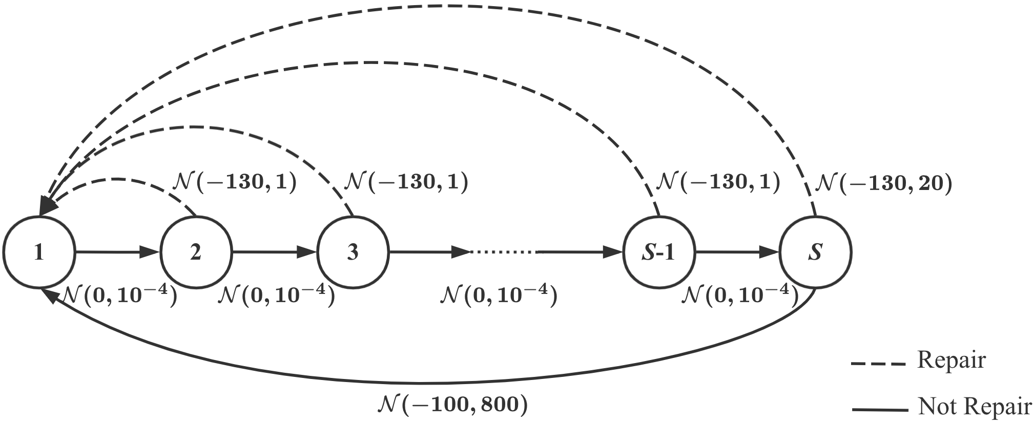
In this experiment, each machine is subject to the same underlying MDP with a state set with and an action set with only two actions: repair the machine or not. The transition is deterministic and the discount factor is . The reward depends on both the current state and action, and all the rewards are independently and normally distributed. Figure 6 illustrates the true underlying distribution that generates the random rewards.
H.4 Additional Results of the Simulation Study
H.5 Additional Results of the Empirical Study
Appendix I Related Works
Table 2 summarizes literature that is related to our work. We remark that, compared to its related works in Table 2, our return-risk model is the only one that considers risk ambiguity, and we have also designed a fast first-order algorithm to obtain its solution, which enhance the practicality of our model for large-scale problems.
| Paper | Uncertainty | Robustness | Ambiguity set | Risk measure | Soft-robustness | |||
|---|---|---|---|---|---|---|---|---|
| Delage and Mannor 2010 |
|
- | - | VaR | No | |||
| Xu and Mannor 2010 |
|
DRO | Nested | - | No | |||
| Yu and Xu 2015 |
|
DRO | (General) Nested | - | No | |||
| Brown et al. 2020 | Rewards | - | - | CVaR | Yes | |||
| Gilbert et al. 2017 | Rewards | - | - | VaR | No | |||
| Lobo et al. 2020 | Transition kernel | - | - | CVaR | Yes | |||
| Yang 2020 | Transition kernel | DRO | Wasserstein | - | No | |||
| This paper | Rewards | DRO | Wasserstein | VaR | Yes |