2021
When using LiDAR semantic segmentation models for safety-critical applications such as autonomous driving, it is essential to understand and improve their robustness with respect to a large range of LiDAR corruptions. In this paper, we aim to comprehensively analyze the robustness of LiDAR semantic segmentation models under various corruptions. To rigorously evaluate the robustness and generalizability of current approaches, we propose a new benchmark, including two corruption datasets SemanticKITTI-C and SemanticPOSS-C, which feature 16 out-of-domain LiDAR corruptions in three groups, namely adverse weather, measurement noise and cross-device discrepancy. Then, we systematically investigate 11 LiDAR semantic segmentation models, especially spanning different input representations (e.g., point clouds, voxels, projected images, and etc.), network architectures and training schemes. Through this study, we obtain two insights: 1) We find out that the input representation plays a crucial role in robustness. Specifically, under specific corruptions, different representations perform variously. 2) Although state-of-the-art methods on LiDAR semantic segmentation achieve promising results on clean data, they are less robust when dealing with noisy data. Finally, based on the above observations, we design a robust LiDAR segmentation model (RLSeg) which greatly boosts the robustness with simple but effective modifications. It is promising that our benchmark, comprehensive analysis, and observations can boost future research in robust LiDAR semantic segmentation for safety-critical applications.
Benchmarking the Robustness of LiDAR Semantic Segmentation Models
keywords
Robustness, LiDAR Corruption, Out-of-distribution, Point Clouds, Semantic Segmentation.
1 Introduction
Autonomous driving, one of the most promising applications for computer vision, has achieved impressive progress in recent studies, where LiDAR semantic segmentation plays a crucial role Hu \BOthers. \APACyear2022; Yan \BOthers. \APACyear2022; Unal \BOthers. \APACyear2022. Current semantic segmentation models are generally evaluated on clean validation sets, which share the same data distribution with the corresponding training sets, e.g., collected with the same sensor, at a similar time and weather condition, and at the same place Behley \BOthers. \APACyear2019. However, due to the inaccurate data acquisition Yan \BOthers. \APACyear2020; Ren \BOthers. \APACyear2022 and complex scenarios caused by diverse weather conditions Hahner \BOthers. \APACyear2019; Hahner \BOthers. \APACyear2022\APACexlab\BCnt1, LiDAR point clouds inevitably suffer from severe corruptions in real-world deployment. Since autonomous driving is a safety-critical application, robustness against out-of-distribution (OOD) LiDAR data becomes an important part of the model.
Understanding and analyzing the robustness of models for image corruption is a well-studied topic, in which several benchmarks are proposed for different tasks, e.g., classification Hendrycks \BBA Dietterich \APACyear2019; Hendrycks \BOthers. \APACyear2021, semantic segmentation Kamann \BBA Rother \APACyear2020, instance segmentation Altindis \BOthers. \APACyear2021 and etc. Generally, these studies simulate corruption through changing RGB values on the original image, resulting in different kinds of perturbations. Moreover, since images are represented as dense pixel arrays, previous works focus on investigating different architectures without modifying the representation of the input. In contrast, analyzing robustness against LiDAR corruption is a more complicated problem: 1) LiDAR point clouds are usually textureless and irregular, and they describe the 3D shapes only through scattered points. Also, point clouds collected by different type of LiDARs may have different ranges and resolutions. Therefore, the corruption on point clouds not only needs to consider the deformation, disturbance and occlusion in the 3D space, but also the domain discrepancy caused by different devices during the data acquisition. 2) Semantic segmentation models in LiDAR scenarios usually adopt diverse representations to meet different requirements. For instance, projection-based methods Milioto \BOthers. \APACyear2019; Y. Zhang \BOthers. \APACyear2020 project LiDAR point clouds onto 2D pixels, and thus enable the application of normal 2D-CNNs. Voxel-based approaches conduct voxelization and transform the LiDAR point clouds into 3D voxel grids Graham \BBA van der Maaten \APACyear2017; Zhou \BOthers. \APACyear2020, exploiting 3D-CNN to capture the fine-grained 3D information. There are also point-based methods Thomas \BOthers. \APACyear2019; Hu \BOthers. \APACyear2020 that learn the geometric details directly on raw point clouds. Recent studies even combine different representations to boost the performance Tang \BOthers. \APACyear2020; Xu \BOthers. \APACyear2021, which makes it more difficult to analyze robustness purely from the architectures.
In this paper, we try to break through the barrier of robust LiDAR semantic segmentation and extend the exploration of model robustness against 3D vision. We find out that the study of corruption robustness on 3D point cloud is still in its infancy. Specifically, most studies Yan \BOthers. \APACyear2020; Ren \BOthers. \APACyear2022 for robustness on 3D point clouds tend to test their models on synthesis datasets, e.g., ModelNet40. The point clouds on these datasets are sampled from CAD models of stand-alone objects. Therefore, the findings in these studies cannot be directly applied to real-world applications, where raw point clouds are collected in large and complex environments. Though a few prior works are related to the model robustness on real-world data (e.g., Lai \BOthers. \APACyear2022), they only conduct a coarse comparison at the level of full models, without analysis on the inner structures and the input representations. As a result, there is no benchmark for robustness in the real-world point clouds, especially for the safety-crucial LiDAR semantic segmentation.
For the first time, based on popular LiDAR semantic segmentation datasets, i.e., SemanticKITTI Behley \BOthers. \APACyear2019 and SemanticPOSS Pan \BOthers. \APACyear2020, we build systematically-designed robust benchmarks with several real-world and out-of-domain corruptions, namely SemanticKITTI-C (in Fig. 1) and SemanticPOSS-C. Following previous studies, the term robustness refers to training a model on clean data and validating it on corrupted data, and thus we respectively introduce diverse corruptions on 4,071 and 500 LiDAR scans in their validation sets. Specifically, the benchmark covers 16 kinds of corruptions in total, which can be categorized into three classes, namely adverse weather, measurement noise, and cross-device discrepancy. To make the benchmark more rigorous, we set several subclass corruptions in each class. For instance, the adverse weather class contains LiDAR scans in snowfall and fog simulations, and there are three independent levels in each corruption, indicating different snowy or foggy intensities. Built upon this benchmark, we further evaluate the robustness of current LiDAR semantic segmentation methods, including analysis of different representations, architectures, and training schemes.
Consequently, we obtain 12 observations in total from various aspects: Representation: We find out that projection-based methods are vulnerable to adverse weathers, especially fog simulation, but they are more robust to local distortion. We also observe that exploiting larger image size in range projection improves the robustness of projection-based methods. Inversely, point-based approaches are vulnerable to local distortion but more robust in different weather conditions. Compared with the above two mainstreams, the voxel representation enjoys impressive robustness in most corruptions. And using cylinder voxel partition Zhou \BOthers. \APACyear2020 is much more robust than using the traditional grids Graham \BBA van der Maaten \APACyear2017. Architecture: 1) For point-based approaches, pseudo kernel local aggregation (e.g., KPConv Thomas \BOthers. \APACyear2019) is the most robust when compared with adaptive-weight Hu \BOthers. \APACyear2020 and MLPs Qi \BOthers. \APACyear2017. Moreover, transformer architectures Zhao \BOthers. \APACyear2021 greatly hamper the robustness of point-based methods. 2) Although hybrid-representation architecture improves the performance on clean data, it makes models more vulnerable to noise, especially for those using MLPs to aggregate point-wised features in each voxel Zhou \BOthers. \APACyear2020; Yan \BOthers. \APACyear2022. Training strategy: Empirically, applying data augmentation such as Mix3D Nekrasov \BOthers. \APACyear2021 improves the robustness. Finally, by identifying the best combination from existing components in terms of input representations, model architectures and data augmentation strategies, we design a robust LiDAR segmentation model (RLSeg) in a simple but effective manner, achieving superior robustness. Our contributions are concluded as follows:
- -
We present the first large-scale robustness benchmark for LiDAR point cloud semantic segmentation under various corruptions, including SemanticKITTI-C and SemanticPOSS-C. The dataset contains 16 corruptions, spanning scenarios in adverse weather conditions, sensor measurement bias and diverse device collections.
- -
We comprehensively study existing methods on our proposed benchmark and analyze the robustness of diverse architectures and representations.
- -
We summarize several effective observations to boost the robustness of LiDAR semantic segmentation. It is identified that architecture and input representation should be carefully considered in future research and real-world deployment.
2 Related Work
2.1 LiDAR Semantic Segmentation
Since the data collected by LiDAR is represented as point clouds, there are several mainstreams to process input point clouds with different representations. More details will be illustrated in Sec. 4.
1) Point-based methods. These approaches directly learn the geometric details on raw point clouds. Generally, they follow the hierarchical architecture as 2D vision, and first conduct sampling strategy in each layer. After that, they search neighboring points from each sampled point, and apply feature aggregation in each local group. The local aggregation function is essential for the point-based methods, and thus many studies design different operators to capture the local geometrics. For instance, point-wise MLP Qi \BOthers. \APACyear2017, adaptive weight W. Wu \BOthers. \APACyear2019; Wang \BOthers. \APACyear2019; Y. Liu \BOthers. \APACyear2019 and pseudo grid Thomas \BOthers. \APACyear2019; Hua \BOthers. \APACyear2018 are utilized to extract local features of point clouds, and they also exploit nonlocal operators Yan \BOthers. \APACyear2020 or attention mechanism Engel \BOthers. \APACyear2021 to learn permutation-invariant dependency. However, point-based methods are not efficient in the LiDAR scenario since their sampling and grouping algorithms are generally time-consuming.
2) Projection-based methods. These methods are very efficient on LiDAR processing since they project the raw point cloud onto a 2D image plane. Previous works project points through plane projection Tatarchenko \BOthers. \APACyear2018, spherical projection B. Wu \BOthers. \APACyear2018; B. Wu \BOthers. \APACyear2019 or both Liong \BOthers. \APACyear2020. Since the projection process inevitably causes the loss of information, the recent studies adopt point-based branches to obtain fine-grained features Alonso \BOthers. \APACyear2020 or refine the segmentation results Qiu \BOthers. \APACyear2022.
3) Voxel-based methods. These approaches are most widely adopted, since they can achieve impressive performance while keep efficient. Generally, they first conduct voxelization, and divide the raw points into different voxel grids. After that, they conduct 3D convolution in the input volumetric. The sparse convolution (SparseConv) Graham \BOthers. \APACyear2018 is the core technique in voxel-based methods. Since there are a large proportion of voxels are empty during the voxelization, which introduce huge computational burden. The core of SparseConv is only conduct operation in non-empty grids, which will be saved in sparse Hash codes. Recent studies adopt SparseConv to design diverse architectures. For instance, Zhou \BOthers. \APACyear2020 design the original grid voxels to cylindrical ones and propose an asymmetrical network to learn anisotropy features. Recently, R. Cheng \BOthers. \APACyear2021 design a multi-branch component with several kernel sizes, capturing features with different receptive field and fusing them through an attention mechanism.
4) Hybrid-representation methods. Though voxel-based methods achieve superior performance, there is still missing geometric during the voxelization process. Hence, there is a trend of exploiting multi-representation fusion. These methods combine multiple representation inputs (i.e., points, projection images, and voxels) and apply feature fusion among different representations. Specifically, Tang \BOthers. \APACyear2020 designs point-voxel CNN operator, which combines point-wise MLPs in each sparse convolution block, and adopts neural architecture search (NAS) to search a more powerful architecture. Xu \BOthers. \APACyear2021 utilizes the above three representations and proposes a range-point-voxel fusion network. Recently, Yan \BOthers. \APACyear2022 applies cross-modal knowledge distillation, introducing prior information from texture and color images during the training phrase. Nevertheless, the hybrid-representation architecture makes them less robust in out-of-domain corruptions
| Corruption (C) | Intensity (I) | Description |
|---|---|---|
| (1) Fog Simulation | Light | Fog simulation with |
| Moderate | Fog simulation with beta | |
| Heavy | Fog simulation with beta | |
| (1) Snowfall Simulation | Light | Snowfall simulation with snowfall rate of 0.5mm/h |
| Moderate | Snowfall simulation with snowfall rate of 1.5mm/h | |
| Heavy | Snowfall simulation with snowfall rate of 2.5mm/h | |
| (2) Global Outliers | Light | 0.1% extra noisy points uniformly in the 3D space |
| Moderate | 5% extra noisy points uniformly in the 3D space | |
| Heavy | 50% extra noisy points uniformly in the 3D space | |
| (2) Local Distortion | Light | 20% points with randomly jitter distortion |
| Moderate | 20% points with randomly jitter distortion | |
| Heavy | 20% points with randomly jitter distortion | |
| (3) Cross 32-beam Device | Dense | Reduce LiDAR beams to 32 |
| Sparse | Reduce LiDAR beams to 32, sample 1/2 points in each beam | |
| (3) Cross 16-beam Device | Dense | Reduce LiDAR beams to 16 |
| Sparse | Reduce LiDAR beams to 16, sample 1/2 points in each beam |
2.2 Robustness Benchmarks for Images
There are comprehensive robustness benchmarks for 2D image processing, spanning different tasks such as classification, semantic segmentation and instance segmentation. For robust image classification, ImageNet-C Hendrycks \BBA Dietterich \APACyear2019 is the pioneer for these field, which corrupts the ImageNet Deng \BOthers. \APACyear2009’s test set with simulated corruptions such as motion blur, adverse weather and noises. After that, ObjectNet Barbu \BOthers. \APACyear2019 build a benchmark with diverse corruptions in rotation, background and viewpoint, and ImageNetV2 Recht \BOthers. \APACyear2019 follow ImageNet and re-collects a test set to benchmark the robustness against natural distribution shift. Recently, ImageNet-A and ImageNet-R are proposed by Hendrycks \BOthers. \APACyear2021, which benchmarks classifier’s robustness against natural adversarial examples. Since ImageNet is initially proposed for diverse tasks, there also exists preliminary attempts to benchmark the robustness of model trained on ImageNet to other downstream tasks, such as semantic segmentation Kamann \BBA Rother \APACyear2020, instance segmentation Altindis \BOthers. \APACyear2021 and object detection Yamada \BBA Otani \APACyear2022. In the field of autonomous driving, there are also existing works producing corruptions on Cityscapes Cordts \BOthers. \APACyear2016, e.g., investigating models’ robustness against adverse weathers Porav \BOthers. \APACyear2020; Sakaridis \BOthers. \APACyear2018 or other corruptions Michaelis \BOthers. \APACyear2019. Recently, ACDC Sakaridis \BOthers. \APACyear2021 dataset collects four common adverse conditions in self-driving, i.e., fog, nighttime, rain, and snow, evaluating the models’ robustness against these real-world corruptions. However, since the difference between 2D-3D data and model architecture, there is still huge demands of a comprehensive 3D robustness benchmark for semantic segmentation.
2.3 3D Robustness Benchmarks
In the field of autonomous driving, there lacks a robustness benchmark for LiDAR semantic segmentation to the best of our knowledge. Existing surveys mostly focus on the point cloud classification task. For instance, Xiao \BBA Wachs \APACyear2021 and Z. Zhang \BOthers. \APACyear2022 propose disturbance and rotation invariant feature extraction, however, they cannot achieve state-of-the-art performance on the clean dataset. Other works boost models’ robustness against adversarial corruptions by denoising and upsampling Zhou \BOthers. \APACyear2019, voting on subsampled point clouds H. Liu \BOthers. \APACyear2021, and applying local relative position Dong \BOthers. \APACyear2020. There are robustness benchmarks for point cloud classification. Specifically, RobustPointSet Taghanaki \BOthers. \APACyear2020 and PointCloud-C Ren \BOthers. \APACyear2022 evaluate the robustness of point cloud classifiers under different corruptions. However, these approaches test robustness against corruptions purely on synthesis dataset, i.e., ModelNet40, and thus the obtained experience and conclusions are often unreliable in real-world self-driving applications.
There are also investigations to improve the robustness on LiDAR scenarios. PointASNL Yan \BOthers. \APACyear2020 proposes adaptive sampling, which adaptive shifts the outlier points onto objects’ surfaces, and thus boosts the robustness against noisy point clouds. In recent year, there are studies investigating performance of object detector in different adverse weathers, where they aim at mitigating the rarity of adverse weather effects. Specifically, Hahner \BOthers. \APACyear2021 and Hahner \BOthers. \APACyear2022\APACexlab\BCnt2 independently propose fog and snowfall simulation, greatly boosting the robustness of object detection models on real-world adverse weathers. However, there is no real-world or simulated adverse weather data set for LiDAR semantic segmentation at present. Moreover, there exists preliminary attempts to investigate the robustness issue of the fusion methods for 3D object detection Bai \BOthers. \APACyear2022; Y. Li \BOthers. \APACyear2022; Yu \BOthers. \APACyear2022. Concretely, TransFusion Bai \BOthers. \APACyear2022 evaluates the robustness of different fusion strategies under several scenarios, e.g., daytime and nighttime, DeepFusion Y. Li \BOthers. \APACyear2022 test the model robustness by adding noise to LiDAR reflections and camera pixels and Yu \BOthers. \APACyear2022 proposes a robust benchmark for LiDAR-camera fusion, which analyzes seven cases of robustness scenarios.
By contrast, we rigorously investigate the LiDAR system and identify three categories, in a total of 16 LiDAR corruptions for semantic segmentation, and develop a toolkit that transforms the existing dataset into a robustness benchmark. We hope our study can boost future research to benchmark the robustness, and give researchers more insights about designing a robust semantic segmentation model.
3 Corruptions Taxonomy
Real-world LiDAR scans can suffer from a wide range of corruptions, based on which we provide a taxonomy of the corruptions. In this paper, we categorize common LiDAR corruptions into three domains, i.e., adverse weather conditions, measurement noise and cross-device discrepancy, in which we produce total six corruptions with 16 severity levels. By applying these six types of corruptions to SemanticKITTI Behley \BOthers. \APACyear2019, we generate two corrupted dataset, i.e., SemanticKITTI-C and SemanticPOSS-C, which is summarized in Tab. 1. In the remaining sections, we will introduce each corruption.

A point cloud is a set of points , where is the number of points and includes the XYZ coordinates of the point . A corruption operation is defined as a set-to-set function:
| (1) |
which maps the clean point cloud and its -dimensional features (if exist) to corrupted ones (e.g., ). For LiDAR point cloud, each is associated with an intensity value , indicating the return strength of a laser beam. In this paper, the intensity is utilized to generate corrupted data, but we do not purely investigate the corruption of intensity.

3.1 Adverse Weather
In this section, we analyze two common weather conditions, namely fog and snowfall. For fog simulation, we follow Hahner \BOthers. \APACyear2021 to add fog to clean-weather point clouds by disturbing points’ positions and intensities according to physically valid rules. Specifically, for a point captured in the clean weather, we first calculate its attenuated response in fog:
| (2) |
where is ’s coordinate in the ego frame and is its measured intensity, is the attenuation coefficient in foggy weather, denotes the distance between the point and the origin. Following Hahner \BOthers. \APACyear2021, we uniformly sample from [0, 0.005, 0.01, 0.02, 0.03, 0.06] when applying fog simulation to each sample. After that, we use the simulation terms in Hahner \BOthers. \APACyear2021 to compute the maximum fog response and its location , which lies in the line connecting the sensor and . Note that the magnitude of is controlled by a backscattering coefficient , which is manually set during the simulation. As shown in Tab. 1, we choose from [0.005, 0.06, 0.2] to conduct fog simulation with different levels. Finally, the updated point position and its intensity are given by:
| (3) |
| (4) |
In other words, if the fog is thick enough to overshadow the solid object point (), we use the fog response (the intensity and position) to replace the original one. Otherwise, we keep the position of the original response with an attenuated intensity.
The overall idea of this snowfall simulation is similar to that of the fog simulation. But unlike fog that homogeneously spreads in the 3D space, snowflakes are treated as opaque particles and are discretely distributed in space without intersecting with each other. For snowfall simulation, we follow Hahner \BOthers. \APACyear2022\APACexlab\BCnt2 to sample snow particles for each LiDAR line and use them to modify the return for each LiDAR beam accordingly. The sampling function samples snow particles according to a given snowfall rate (mm/h), which controls the number of particles in a certain range. As shown in Tab. 1, we separately set the snowfall rate to 0.5/1.5/2.5 to simulate light/moderate/heavy snowfall.
The above two weathers have different characteristics. For instance, there are large areas of noisy points distributed around the sensor in foggy weather, and makes objects sparser due to the occlusion, especially for the remote objects. As illustrated in Fig. 2, the number of these noisy points grows as the intensity of fog increases. Moreover, the noise introduced by fog is not uniformly distributed around the sensor. The presence of noise depends on whether there is any object in the line of sight below a certain range from the sensor. Generally, there will be few spurious returns from the respective pulses if a solid object exists at a moderate range. Inversely, if there is no object in a certain range, there are a lot of spurious returns that are caused by fog. As for the snowfall, there are two explicit characteristics. On the one hand, the snow particles are explicitly modeled as opaque spheres, whose sizes are controlled by the snowfall rate. As shown in Fig. 3, compared with foggy LiDAR where the noisy points are almost around the sensor, the noisy points in snowfall conditions are distributed more uniformly. Also, the snowfall rate does not greatly affect the number of noisy points but the size of snowy particles. On the other hand, wetness on the ground will exist in snowfall, where the emerging thin water layer increases the specular component of reflection by the ground surface. To sum up, these two corruptions impact the models through global noisy points, making remote points sparser. Nevertheless, they generally have different patterns.
3.2 Measurement Noise
Besides adverse weather, noises may also appear when corruption occurs during the data transmission or the sensors fail to capture information properly. On one hand, due to the sensor overheated, false activations at max-distance makes a large number of noise points in the 3D space. On the other hand, external disturbances, e.g., bumpy surfaces, dust, insects, that often lead to nonnegligible motion blur in local regions. We model such data disturbance using two types of random noises, as shown in Fig. 4. Note that we only consider point coordinates during such corrupting operations.
Global outliers. We randomly sample noises in a unit sphere and then merge them into a clean point cloud with proper rescaling. Such noises span the whole scene globally and are not conditional on the geometry of the clean point cloud. Formally, given the clean point cloud , the corrupted point cloud is obtained by:
| (5) |
where denotes sampled noises and . We control the noise intensity by selecting the proportion of noises from [0.1%, 5%, 50%] as shown in Tab. 1.
Local distortion. We randomly select some points within a scene and add Gaussian noises to their coordinates. Unlike global noises, which add additional points to a scene, local noises do not change the number of points. Compared to global noises, local noises jitter around a local neighborhood of the original points, mimicking the noisy disturbance during the data collection. Formally, the local distortion point cloud is given by:
| (6) | |||
where randomly sample points from the clean point cloud . denotes the random offsets sampled from a Gaussian distribution . and are element-wise addition and set exclusion, respectively. As shown in Tab. 1, we choose from [0.05, 0.1, 0.2] to control the jittering range in three different levels. The proportion of noises is 20%


| Mainstream | Method | Main representation | Extra representation | Reference |
|---|---|---|---|---|
| Projection-based | SalsaNext Cortinhal \BOthers. \APACyear2020 | Range image | - | ArXiv 2020 |
| PolarNet Y. Zhang \BOthers. \APACyear2020 | BEV image | - | CVPR 2020 | |
| CENet H\BHBIX. Cheng \BOthers. \APACyear2022 | Range image | - | ICME 2022 | |
| GFNet Qiu \BOthers. \APACyear2022 | Range and BEV images | Point cloud | TMLR 2022 | |
| Point-based | KPConv Thomas \BOthers. \APACyear2019 | Point cloud | - | ICCV 2019 |
| RandLANet Hu \BOthers. \APACyear2020 | Point cloud | - | CVPR 2021 | |
| Point Transformer Zhao \BOthers. \APACyear2021 | Point cloud | - | ICCV 2021 | |
| Voxel-based | MinkowskiNet Choy \BOthers. \APACyear2019 | Grid voxel | - | CVPR 2019 |
| SPVCNN Tang \BOthers. \APACyear2020 | Grid voxel | Point cloud | ECCV 2020 | |
| Cylinder3D Zhou \BOthers. \APACyear2020 | Cylinder voxel | Point cloud | CVPR 2021 | |
| 2DPASS Yan \BOthers. \APACyear2022 | Grid voxel | Point cloud | ECCV 2022 |
3.3 Cross-Device Discrepancy
An ideal segmentation algorithm is supposed to be robust across different devices with various specifications. While multiple factors (e.g., beam number and scanning speed of the LiDAR sensors) cause cross-device domain shifts, we focus on the beam number in this paper. To ensure high-quality data annotation, most large-scale datasets Geiger \BOthers. \APACyear2012; Sun \BOthers. \APACyear2020 are collected using high-resolution LiDARs. However, due to prohibitive costs, most practical vehicles are only shipped with low-beam sensors. For instance, KITTI Geiger \BOthers. \APACyear2012 collects data through 64-beam LiDAR and each beam contains 1863 points in average, while those parameters in NuScenes Caesar \BOthers. \APACyear2020 are 32-beam and 1084 points. This suggests that an ideal segmentation model should be able to robust to different data distributions generated by different sensors. Unlike other factors introduced in previous subsections, the beam-induced domain gap is directly caused by the cross-device discrepancy instead of the collecting environment, making it also very important in our robustness analysis.
To include the beam-based cross-device discrepancy in our benchmark dataset, we downsample the high-beam data (i.e., 64-beam) to low-beam data (e.g.., 16-, 32-beam) using beam-level downsampling as shown in Fig. 5. One necessary information needed for beam-level downsampling is the beam label for each point, which is usually unknown for most datasets. To this end, we first assign a beam label to each point according to its zenith value in the spherical coordinate, which can be obtained via the following conversion:
| (7) |
where is the Cartesian coordinate of the point and the and are zenith and azimuth angles. Following Wei \BOthers. \APACyear2022, we obtain beam labels by applying K-Means clustering on the zenith angles, where the number of clusters is set as the actual beam number of the high-beam point cloud. Compared to assigning beam labels by putting zenith angles into evenly distributed bins, the clustering-based technique does not require a pre-define zenith range and thus is more robust across different datasets. For a high-beam point cloud with the beam labels, we can easily downsample it into data with any lower beam number. In practice, we downsample point clouds with the beam numbers of 32 and 16. To simulate the diverse spinning speeds of the LiDAR devices, we evenly downsample points in each beam according to their azimuth angles. By combining the above simulation, we have four corrupted data generated in Tab. 1.
4 Candidate Methods
We benchmark 11 existing methods for LiDAR semantic segmentation, as shown in Tab. 2. Though we treat hybrid-representation methods as an independent mainstream in Sec. 2.1, current voxel-based and projection-based methods widely incorporate additional representations for auxiliary learning. Therefore, we categorize them only according to their main input representation, and the extra-representation will be illustrated if existed.
4.1 Projection-based Methods
In this paper, we choose SalsaNext Cortinhal \BOthers. \APACyear2020, PolarNet Y. Zhang \BOthers. \APACyear2020, CENet H\BHBIX. Cheng \BOthers. \APACyear2022 and GFNet Qiu \BOthers. \APACyear2022 as the typical approaches of the projection-base method. These models project a LiDAR point cloud into 2D images and apply a 2D convolutional neural network for semantic segmentation. Among the above methods, SalsaNext Cortinhal \BOthers. \APACyear2020 and CENet H\BHBIX. Cheng \BOthers. \APACyear2022 conduct sphere projection to gain range views (RV), PolarNet Y. Zhang \BOthers. \APACyear2020 adopts polar projection to obtain bird’s-eye-view (BEV) under a polar coordinate system, and GFNet Qiu \BOthers. \APACyear2022 uses the both.
Sphere projection for range-view. We denote the number of points in the LiDAR point cloud and are the height and width of the projected image. As shown in Fig. 6, the spherical projection maps each point to an image coordinate via
| (8) |
where and are the -th point and its coordinates on the range image plane. is the range of each point and is the vertical field-of-view of the sensor. Finally, the LiDAR point cloud is converted to a range image with the shape of . The channel is generally , including , , , and of the point.
Polar projection for bird’s-eye-view. Existing methods also project the LiDAR point cloud to the bird’s-eye-view (BEV) through a top-down orthogonal projection. Considering the imbalanced spatial distribution in LiDAR data, polar projection first transforms the BEV from the Cartesian system into a polar coordinate system through
| (9) |
where is the coordinate transformation from the Cartesian system to the polar system. After that, they discretize to and and obtain a BEV image.

Architectures. Since the LiDAR point cloud is already mapped onto an image plane, typical 2D semantic segmentation networks can be directly adopted. Specifically, U-Nets Ronneberger \BOthers. \APACyear2015 with specific modifications are applied in previous methods. 1) Approaches with range images do not conduct pooling in height dimension due to the large width-height ratio of the input, as shown in Fig. 6. 2) SalsaNext utilizes an additional pixel-shuffle layer in the last encoder, and CENet conducts multiscale supervision in encoder and decoder layers. 3) PolarNet applies a hybrid-representation manner, i.e., designing a PointHead (will be described in Sec. 5.4) in the initial stage, which aggregates the features of original points into each BEV pixel, and finally conducts semantic segmentation through the 2D U-Net. 4) GFNet Qiu \BOthers. \APACyear2022 has a two-branch architecture, where two U-Nets independently encode the features of range-view (RV) and bird’s-eye-view (BEV). There are several Geometric Flow (GF) modules between their decoder layers with different scales, which update each other’s features by fusing the features of both branches. Finally, it utilizes a hybrid-representation manner, aggregating the features of two branches in their last layers and feeding the fused feature into KPConv Thomas \BOthers. \APACyear2019 to gain point-wise predictions.
Configurations. In our experiments, we adopt the official architectures of projection-based methods (i.e., SalsaNext11 1 https://github.com/TiagoCortinhal/SalsaNext, CENet22 2 https://github.com/huixiancheng/CENet, PolarNet33 3 https://github.com/edwardzhou130/PolarSeg and GFNet44 4 https://github.com/haibo-qiu/GFNet). Note that CENet is trained with a multi-stage strategy, which trains with range image for the initial stage, and fine-tunes the pre-trained model aggressively on and ones. Since the official codes on SemanticKITTI only provide the checkpoint on range images, we fine-tune the checkpoint on larger ones through provided configurations. In contrast, SalsaNext directly trains their model on range images. As for the PolarNet, it first crops points of the polar coordinate system in the range from [3, , -3] to [50, , 1.5], and then discretize points into a [480,360] BEV partition. GFNet combines RV and BEV representation, utilizing both range images and BEV plane. The training setup on SemanticPOSS is the same as that on SemanticKITTI.
4.2 Point-based Methods
Point-based approaches aim at extracting features on raw point clouds directly, as shown in Fig. 7. In this paper, KPConv Thomas \BOthers. \APACyear2019, RandLA-Net Hu \BOthers. \APACyear2020 and Point Transformer Zhao \BOthers. \APACyear2021 are selected as our candidate methods. Specifically, these methods first apply sampling approaches to select target points from the original point clouds, and then conduct local aggregation on each target point and mine local geometrics, as Fig. 7(a) shows. After constructing a hierarchical architecture in Fig. 7(b), point-based methods gain the global semantic information of the input point cloud.
General formulation of local aggregation. Let and denote the coordinate and feature of the -th point. In general, for each , a local aggregation function first transforms its neighbor with feature into a new feature by a transformation function , and then aggregates all transformed neighborhood features to generate an updated feature of via an aggregation function :
| (10) |
In practice, represents the neighborhood index of point . According to the category to which the transformation function belongs, previous local aggregation approaches can be roughly categorized into four classes: 1) Point-wise MLP based, 2) Adaptive weight based, 3) Pseudo grid based and 4) Transformer based approaches. The typical one of the first class is PointNet++ Qi \BOthers. \APACyear2017, where and are and max pooling respectively, in which is concatenation operation. However, directly learn the 3D shapes through simple point-wise MLP and pooling cannot work well in the LiDAR scenario, i.e., it only achieves 20% mIoU on SemanticKITTI in previous studies Behley \BOthers. \APACyear2019. Therefore, we did not adopt this kind of methods in our paper.
Adaptive weight based methods. The adaptive weight based methods design diverse convolution filters over arbitrary relative positions and hence compute weights on all neighbor points. RandLA-Net Hu \BOthers. \APACyear2020 is a typical one in adaptive weight based methods. Concretely, its transformation function can be represented as
| (11) |
where calculates the Euclidean distance between the neighboring and center points. After that, it aggregates the neighboring features through attention mechanism Vaswani \BOthers. \APACyear2017, which first calculates an attention weight according to the feature, and then conducts weighted average.
Pseudo grid based methods. KPConv Thomas \BOthers. \APACyear2019 is a representative pseudo grid based method, which generates pseudo features on several sampled regular grid points, and thus regular convolution methods can play a normal role. Specifically, it samples equally distributed spherical grid points in the 3D space, in which the pseudo features on the -th grid point can be calculated as
| (12) |
where each grid point has a strict mapping with the relative position to the center point. is a hyperparameter. After that, the transformation function in pseudo grid based methods can be formulated as
| (13) |
where is a parametrized weight in the convolution operator and defined on each grid point. Finally, after applying max pooling as aggregation function , it updates the feature of each target point through aggregating features in local neighbors.
Transformer-based methods. Besides analyzing traditional local aggregation based approaches, we also adopt a recent transformer-based method (i.e., Point Transformer Zhao \BOthers. \APACyear2021) in this paper. The point transformer layer is based on vector self-attention, which uses the subtraction relation and there is a position encoding in both the attention vector and the transformed features . Specifically, in each local group (i.e., ), the transformation function in a transformer based method can be formulated as
| (14) |
where , , , are independent MLPs. is a positional encoding in self-attention, allowing the operator to adapt to local structure. After updating the neighboring features, Point Transformer utilizes a summation function as an aggregation function to fuse features.
Architectures. All above three methods follow the widely-used UNet-like encoder-decoder architecture with skip connections. The LiDAR point cloud is first fed to a shared MLP layer to extract per-point features. Encoder and decoder layers are then used to learn features for each point. Finally, fully-connected layers are used to predict the semantic label of each point. KPConv and RandLA-Net utilize stacked two corresponding local aggregation in each encoder layer, while Point Transformer using the combination of point-wise MLP with point transformer layer. In decoder layers, all method interpolate the sampled points and update features through point-wise MLPs. Moreover, RandLA-Net uses random sampling in each local aggregation, while other two utilizing uniformly sample points. For KPConv and RandLA-Net, we adopt their official architectures on SemanticKITTI dataset (four encoders and decoders). As for the Point Transformer, since it is only designed for indoor semantic segmentation, we adopt original architecture with five encoders and decoders.
Configurations. During the training, both KPConv55 5 https://github.com/HuguesTHOMAS/KPConv-PyTorch and RandLA-Net66 6 https://github.com/QingyongHu/RandLA-Net follow their official configurations on SemanticKITTI. To accelerate the training phrase, they first conduct grid sampling with grid size 0.06 to gain a small sub-cloud. Moreover, they respectively crop patches with a 4 radius and 50,000 points in each training iteration. During the inference, they inference through small patches util each of the points have been inferred three times. Since there are not published codes on SemanticKITTI and SemanticPOSS for Point Transformer77 7 https://github.com/POSTECH-CVLab/point-transformer, we utilize the same configurations as Tang \BOthers. \APACyear2020 during the training and inference.
4.3 Voxel-based Methods
Since voxel-based methods are the most popular mainstream for LiDAR semantic segmentation now, we select four methods (i.e., MinkowskiNet Choy \BOthers. \APACyear2019, SPVCNN Tang \BOthers. \APACyear2020, Cylinder3D Zhou \BOthers. \APACyear2020 and 2DPASS Yan \BOthers. \APACyear2022) in this paper.
Grid partition. Voxel-based methods exploit voxelization and transform the LiDAR point cloud into 3D voxels, such that the 3D convolutions can be applied. Specifically, they shift all the points to the local coordinate system with the geometric center as the origin. Then, all the points are normalized into a unit sphere and scaled to the range of , where the normalized coordinates are denoted as . After that, they transform the normalized point cloud to a voxel representation with voxel size ( is voxelized feature representation):
| (15) | ||||
where is the floor function, and is a binary indicator of whether belongs to the -th voxel grid or not. is the number of points in the -th voxel, and the original point coordinates are averaged as the features of each voxel. After the operations in Eqn. (15), only the non-empty voxels are preserved () in a hash table. The, the convolution operation only conducts on the non-empty voxels, thus maintaining the computational efficiency.
Cylindrical partition. Recent study Zhou \BOthers. \APACyear2020 proposes cylinder partition for voxelization, which makes a higher non-empty proportion and more balanced point distribution compared with grid partition, especially for farther-away regions. In practice, it first transforms the Cartesian system into a polar coordinate system through Eqn. (9), and then conducts voxelization as Eqn. (15).
Architectures. Both MinkowskiNet and SPVCNN88 8 https://github.com/mit-han-lab/spvnas utilize the same U-Net architecture, where the difference is that there is a parallel point-wise MLP branch in the latter. Cylinder3D99 9 https://github.com/xinge008/Cylinder3D proposes asymmetrical 3D convolution networks, in which it constructs several asymmetrical blocks (e.g., exploiting , and kernels in parallel) as unit components. 2DPASS1010 10 https://github.com/yanx27/2DPASS uses a similar encoder architecture as SPVCNN, but it discards the decoder part and predicts the results through multiscale concatenation. Moreover, Cylinder3D and 2DPASS exploit additional a PointHead (will be introduced in Sec. 5.4) to aggregate point-wise features into each voxel.
Configurations. Both Cylinder3D and 2DPASS are tested on SemanticKITTI-C with their released checkpoints. For the SemanticPOSS-C, and retrain them with the same setup as SemanticKITTI. As for the MinkowskiNet and SPVCNN, we re-trained their official architectures with batch size 8 for epoch 64, and gain higher results. All approaches are tested with test-time augmentation (TTA), i.e., rotating the point cloud with 12 views and averaging the predictions.
5 Benchmarking and Analysis
In this section, we benchmark the aforementioned approaches with our diverse set of LiDAR corruptions. We first introduce the experiment setting and evaluation metrics of our benchmark in Sec. 5.1. After that, the benchmark results are shown in Sec. 5.2 to 5.5 with comprehensive analysis. We demonstrate our benchmark results spanning different representation, architecture, corruption intensity and data augmentation. As results, we summarize 12 observations in total. Finally, in Sec. 6, we introduce RLSeg, a robust architecture based on the above observations, which effectively boosts the robustness of LiDAR semantic segmentation.
5.1 Experiment Setting
Dataset. SemanticKITTI is currently the most widely used LiDAR semantic segmentation dataset, which consists of 43,552 densely annotated LiDAR scans belonging to 21 sequences. These scans are annotated with a total of 19 valid classes, and each scan spans up to meters with more than points. Initially, the sequence 00 to 07, 09 to 10 are the training set, 11 to 21 are the test set, and 08 is the validation set. Since the annotations of 11 to 21 are not available offline, we train all approaches on training set and evaluate them on sequence 08.
SemanticPOSS contains 11 similar annotated categories with SemanticKITTI. It is more challenging because each scene contains more than 10 sparse small objects (i.e., people and bicycle), while the total frames number are only 1/20 of SemanticKITTI. We train all approaches on its training set (sequence 00, 01 and 03-05) and evaluate them on sequence 02.
Annotation modification. Since the corrupted point clouds will be sparser or there are new noisy points existed, we slightly modify the original annotations. Specifically, for the corruption data in fog and snowfall simulations, we utilize the noisy data to query the original point of the clean data to annotate labels, labeling points as ‘ignore’ if there is no point existed. In the noisy corruption (i.e., local and global), we directly annotate noisy points as ‘ignore’. In the cross-device scenario, since all the points are sampled from the original LiDAR, there is no demand for modification. Note that the ‘ignore’ class is not considered in the evaluation.
Evaluation metric. To intuitively demonstrate the robustness of candidate methods, we use the performance on each corruption and the relative performance degradation compared to the clean data on our benchmark datasets as our evaluation metrics. Specifically, we adopt mIoU(%) (i.e., averaged Intersection over Union on each class) as our metric and the score on the clean dataset is denoted as . As demonstrated in Tab. 1, we benchmark existing methods with six categories of corruptions (C), spanning 16 different intensities (I). The performance toward certain corruption can be calculated by averaging results on each intensity:
| (16) |
where and are total intensities and the number of intensity in the corruption . denotes the mIoU under corruption and intensity and are the averaged mIoU of all intensities under the corruption . The relative mean robustness performance of the model is defined as . The higher R means the model is more robust to inferior LiDAR conditions. Moreover, we define a robustness mIoU (RmIoU) and averaged relative performance (mR) through averaging the results on different corruption:
| (17) |
| Clean | Robustness | Fog | Snowfall | Global Outliers | Local Distortion | 32-beam | 16-beam | |||||||||
| Method | mIoU | RmIoU | mR | mIoU | R | mIoU | R | mIoU | R | mIoU | R | mIoU | R | mIoU | R | |
| Projection | SalsaNext | 55.8 | 42.7 | 76.5 | 27.3 | 48.9 | 43.6 | 78.1 | 49.5 | 88.7 | 53.6 | 96.1 | 51.1 | 91.6 | 31.0 | 55.6 |
| PolarNet | 58.2 | 43.3 | 74.5 | 31.7 | 54.5 | 47.4 | 81.5 | 52.4 | 90.0 | 48.7 | 83.7 | 46.3 | 79.5 | 33.5 | 57.6 | |
| CENet | 62.3 | 47.7 | 76.6 | 31.5 | 50.5 | 51.3 | 82.4 | 57.2 | 91.7 | 58.6 | 94.0 | 54.5 | 87.5 | 33.4 | 53.7 | |
| GFNet | 63.0 | 46.4 | 73.6 | 31.1 | 49.4 | 41.8 | 66.3 | 61.4 | 97.5 | 56.0 | 88.9 | 52.5 | 83.4 | 35.6 | 56.5 | |
| Point | KPConv | 63.5 | 51.6 | 81.3 | 59.6 | 93.9 | 54.8 | 86.4 | 61.9 | 97.4 | 31.8 | 50.1 | 58.3 | 91.7 | 43.4 | 68.3 |
| RandLA-Net | 59.2 | 47.6 | 80.4 | 56.4 | 95.4 | 50.0 | 84.4 | 57.8 | 97.8 | 26.4 | 44.7 | 53.3 | 90.1 | 41.7 | 70.5 | |
| Point Trans. | 63.3 | 40.5 | 64.0 | 45.5 | 71.9 | 44.2 | 69.9 | 38.8 | 61.4 | 39.3 | 62.2 | 47.2 | 74.6 | 27.9 | 44.2 | |
| Voxel | MinkowskiNet | 66.3 | 53.6 | 80.9 | 56.3 | 84.9 | 50.4 | 76.1 | 65.3 | 98.5 | 37.0 | 55.9 | 62.2 | 93.9 | 50.4 | 76.0 |
| SPVCNN | 67.4 | 53.2 | 78.9 | 53.7 | 79.7 | 50.5 | 75.0 | 65.8 | 97.7 | 39.6 | 58.8 | 61.7 | 91.5 | 47.7 | 70.8 | |
| Cylinder3D | 66.9 | 46.5 | 69.5 | 44.2 | 66.1 | 45.7 | 68.3 | 63.3 | 94.6 | 39.7 | 59.4 | 51.2 | 76.5 | 34.7 | 51.9 | |
| 2DPASS | 70.1 | 51.1 | 72.9 | 40.4 | 57.6 | 53.6 | 76.5 | 69.8 | 99.6 | 43.9 | 62.7 | 61.3 | 87.4 | 37.7 | 53.7 | |
| RLSeg (ours) | 73.5 | 62.5 | 85.0 | 57.6 | 78.4 | 66.2 | 90.1 | 73.4 | 99.9 | 71.9 | 97.8 | 62.3 | 84.7 | 43.6 | 59.3 | |
| Clean | Robustness | Fog | Snowfall | Global Outliers | Local Distortion | 32-beam | 16-beam | |||||||||
| Method | mIoU | RmIoU | mR | mIoU | R | mIoU | R | mIoU | R | mIoU | R | mIoU | R | mIoU | R | |
| Projection | SalsaNext | 49.2 | 31.1 | 63.1 | 21.9 | 44.6 | 6.4 | 13.0 | 37.7 | 76.6 | 48.0 | 97.6 | 42.0 | 85.3 | 30.4 | 61.8 |
| PolarNet | 53.5 | 36.8 | 68.7 | 30.0 | 56.1 | 9.8 | 18.4 | 51.3 | 95.9 | 51.2 | 95.6 | 44.5 | 83.2 | 33.7 | 63.0 | |
| GFNet | 49.0 | 36.2 | 73.9 | 28.2 | 57.4 | 12.9 | 26.3 | 48.9 | 99.9 | 47.5 | 97.0 | 44.1 | 90.1 | 35.7 | 72.8 | |
| CENet | 50.9 | 34.5 | 67.8 | 35.5 | 69.8 | 4.5 | 8.8 | 42.1 | 82.8 | 50.2 | 98.6 | 44.0 | 86.4 | 30.6 | 60.1 | |
| Point | KPConv | 56.3 | 46.9 | 83.3 | 49.3 | 87.6 | 46.8 | 83.2 | 56.3 | 100.0 | 45.6 | 81.0 | 49.5 | 87.9 | 34.0 | 60.3 |
| RandLA-Net | 51.2 | 42.5 | 83.0 | 46.4 | 90.6 | 42.8 | 83.6 | 49.4 | 96.5 | 42.2 | 82.4 | 42.5 | 82.9 | 31.8 | 62.1 | |
| PointTransformer | 57.0 | 35.9 | 63.0 | 34.9 | 61.2 | 19.4 | 34.1 | 52.7 | 92.4 | 48.3 | 84.7 | 37.7 | 66.2 | 22.6 | 39.6 | |
| Voxel | MinkowskiNet | 57.9 | 44.5 | 76.8 | 39.8 | 68.8 | 23.4 | 40.3 | 55.0 | 94.9 | 55.4 | 95.6 | 53.0 | 91.5 | 40.3 | 69.5 |
| SPVCNN | 60.4 | 45.7 | 75.7 | 41.7 | 68.9 | 20.3 | 33.5 | 60.4 | 100.0 | 55.7 | 92.2 | 55.5 | 91.8 | 40.8 | 67.5 | |
| Cylinder3D | 48.7 | 31.1 | 63.9 | 28.4 | 58.5 | 11.8 | 24.3 | 46.4 | 95.3 | 44.3 | 91.0 | 32.8 | 67.4 | 22.9 | 47.1 | |
| 2DPASS | 55.9 | 41.7 | 74.7 | 35.9 | 64.3 | 15.5 | 27.8 | 55.8 | 99.8 | 53.9 | 96.5 | 50.1 | 89.7 | 39.0 | 69.8 | |
| RLSeg (ours) | 59.5 | 50.1 | 84.2 | 47.9 | 80.5 | 48.5 | 81.6 | 59.4 | 99.9 | 58.5 | 98.4 | 51.3 | 86.2 | 34.9 | 58.6 | |

5.2 Main Results
Benchmark results are reported in Tab. 4 and 4, in which projection-based, point-based and voxel-based methods are demonstrated in upper, median and lower parts, respectively. Our proposed solution will be introduced in Sec. 6. According to the table, we have the following discovery:
Observation-1: Projection-based methods are most vulnerable to common corruptions, especially to foggy simulation. However, they are greatly robust to local distortion corruption.
As shown in the tables, existing projection-based methods respectively achieve around 75% and 70% metric of mR on SemanticKITTI-C and SemanticPOSS-C, which is much lower than those of point-based and voxel-based methods. Furthermore, they only achieve around 50% original performance in fog simulation of SemanticKITTI-C and less than 20% in the case of snow simulation on SemanticPOSS-C. In contrast, these methods are extremely robust to local noise, especially for the pure range image based method (i.e., 96.1% and 94.0% R for SalsaNext Cortinhal \BOthers. \APACyear2020 and CENet H\BHBIX. Cheng \BOthers. \APACyear2022 in SemanticKITTI-C, respectively). The reason of the above observation is that the local corruption only slightly affects the range image and the foggy one make range images messy, as shown in Fig. 8. PolarNet Y. Zhang \BOthers. \APACyear2020 and GFNet Qiu \BOthers. \APACyear2022 are not much robust to local corruption, since there are BEV projections in their models. Nevertheless, they still respectively keep 83.7% and 88.9% performance, which is much higher than those of point and voxel based methods.
Observation-2: Traditional point-based methods (RandLA-Net and KPConv) are more robust to common corruptions, compared with projection-based methods. Specifically, they are much robust to adverse weathers, but less robust to local distortion.
The Tab. 4 and 4 illustrate RandLA-Net Hu \BOthers. \APACyear2020 and KPConv Thomas \BOthers. \APACyear2019 respectively achieve 81.3%/83.3% and 80.4%/83.0% in the metric of mR. Especially, they gain highest 93.9% and 95.4% R in the case of fog simulation on SemanticKITTI-C, where the best projection and voxel based methods only achieve 54.5% and 79.7%, respectively. Inversely, they only gain 50.1% and 44.7% performance in local noise of SemanticKITTI-C, which is lower than common performance of other two mainstreams. The reason is that the local distortion protects the local geometric and thus makes the local aggregation failed.
| Noise types | Ratio (%) | SalsaNext | KPConv | MinkowskiNet | |||
| mIoU | R | mIoU | R | mIoU | R | ||
| No corruption | 0 | 55.8 | 100.0 | 63.5 | 100.0 | 66.3 | 100.0 |
| Global outliers | 0.1 | 55.8 | 100.0 | 62.6 | 98.6 | 66.5 | 100.0 |
| 5 | 53.8 | 96.4 | 62.8 | 98.9 | 65.9 | 99.4 | |
| 10 | 51.6 | 92.5 | 62.4 | 98.3 | 64.5 | 97.3 | |
| 20 | 47.4 | 84.9 | 61.8 | 97.3 | 63.9 | 96.4 | |
| 50 | 38.9 | 69.7 | 60.2 | 94.8 | 63.5 | 95.8 | |
| Local distortion () | 10 | 55.7 | 99.8 | 59.8 | 94.2 | 62.1 | 93.6 |
| 20 | 55.2 | 98.9 | 35.5 | 55.9 | 55.5 | 83.7 | |
| 50 | 50.7 | 90.9 | 17.1 | 26.9 | 36.9 | 55.7 | |
| Local distortion () | 10 | 55.4 | 99.3 | 41.6 | 65.5 | 52.3 | 78.9 |
| 20 | 53.7 | 96.2 | 25.6 | 40.3 | 32.3 | 48.7 | |
| 50 | 42.7 | 76.5 | 11.1 | 17.5 | 17.5 | 26.4 | |
| Local distortion () | 10 | 54.8 | 98.2 | 34.1 | 53.7 | 42.5 | 64.1 |
| 20 | 51.9 | 93.0 | 21.2 | 33.4 | 23.8 | 35.9 | |
| 50 | 35.4 | 63.4 | 14.1 | 22.2 | 11.2 | 16.9 | |
| SalsaNext | KPConv | MinkowskiNet | |||||
|---|---|---|---|---|---|---|---|
| LiDAR types | Sparseness | mIoU | R | mIoU | R | mIoU | R |
| 64-beam | Dense | 55.8 | 100.0 | 63.0 | 100.0 | 66.3 | 100.0 |
| Sparse | 52.1 | 93.4 | 63.4 | 99.8 | 63.5 | 95.8 | |
| 32-beam | Dense | 52.4 | 93.9 | 59.0 | 92.9 | 62.5 | 94.3 |
| Sparse | 49.8 | 89.2 | 57.5 | 90.6 | 59.5 | 89.7 | |
| 16-beam | Dense | 32.3 | 57.8 | 43.8 | 69.0 | 50.2 | 75.7 |
| Sparse | 29.7 | 53.2 | 43.0 | 67.7 | 46.4 | 70.0 | |
Observation-3: Transformer-based local aggregation greatly hampers the robustness, especially for global outliers.
Though transformer-based architecture improve the performance on the clean data, it greatly affects the robustness against diverse corruptions. Concretely, Point Transformer Zhao \BOthers. \APACyear2021 gains the lowest result in almost every corruption scenarios. For instance, in the global outliers, most of the approaches can keep above 90% performance, but it only achieves 61.5% on SemanticKITTI-C.
Observation-4: Pure voxel-based method shows most superior robustness cross all corruptions, especially for cross-devices scenario. Recent state-of-the-art voxel-based methods loss their robustness against corruption due to their hybrid-representation architectures.
The results illustrate that MinkowskiNet Choy \BOthers. \APACyear2019 enjoy most superior robustness with pure voxel architecture. Specifically, it achieves 76.0% performance preserve in the case of 16-beam cross-device on SemanticKITTI-C, surpassing those of projection and point based methods over 20% and 10%, respectively. SPVCNN Tang \BOthers. \APACyear2020 introduces point-wise MLP in parallel with voxel architecture, nevertheless, it loses the robustness especially in fog simulation and 16-beam cross-device corruptions. Recent state-of-the-art Cylinder3D Zhu \BOthers. \APACyear2021 and 2DPASS Yan \BOthers. \APACyear2022 have poor generalization ability since they use extra representation. More analysis for this design will be illustrated in Sec. 5.4.
5.3 Robustness in Specific Corruption
In this section, we demonstrate and analyze the result of each specific corruption. To facilitate the experiment, we only select the most typical method in each mainstream, i.e., SalsaNext, KPConv and MinkowskiNet, and test them on SemanticKITTI-C.
Fog simulation. Fig. 9 illustrates the comprehensive results of robustness in fog simulation. Apart from the three intensities related in Tab. 1, i.e., 0.005, 0.06 and 0.2, we also provide other 6 intensities, including 0.01, 0.02, 0.03, 0.1, 0.12, 0.15. We find out that SalsaNext is greatly affected by denser fog, especially when is larger than 0.06. Inversely, KPConv shows its superior robustness crossing different fog intensities. Therefore, we have the following summary:
Observation-5: All types of methods will have performance decay as the fog becomes heavier, among which the projection-based method decreases fastest, and the point-based method decreases slowest.
Snow simulation. Fig. 10 illustrates the detailed results of snow simulation. The conclusion is:
Observation-6: Though snow simulation hampers all types of methods, the performances of point-based and voxel-based methods are slightly decreased as the snow becomes heavier, while the projection-based methods illustrate an inverse tendency, i.e., there are slight performance boosts in heavier snowfall.
The reason may be that the large snowfall makes the scattered noise in the 3D space cover a larger area, thus affecting the point-based and voxel-base methods. However, as shown in Fig. 12, when the 3D scene is mapped to a range image, these scattered points with larger coverage will become sparse in each pixel.
Noisy corruptions. Results in different noisy corruptions are illustrated in Tab. 5. On one hand, MinkowskiNet is the most robust method against global outliers. It even keeps 95.8% performance in the scenario with additional 50% global noisy points. On the opposite, SalsaNext has poor generalization ability for global noise, especially with a larger proportion of noisy points. On the other hand, the projection-based method (i.e., SalsaNext) shows great robustness in local distortion noises, spanning different jittering ranges, as summarized in observation-1. In contrast, KPConv and MinkowskiNet cannot work normally in large-range jittering distortion.
Cross-device discrepancy. We demonstrate concrete results on different LiDAR types in Tab. 6, where MinkowskiNet achieves the best results in cross-device scenarios. In contrast, SalsaNext has poor robustness, especially in 16-beam devices with only around 50% original performance. Furthermore, there is an interesting discovery:
Observation-7: Point-based methods (i.e., KPConv) are greatly robust against the scenario of downsampling points in each LiDAR beam.
As illustrated in the table, removing 1/2 points in each beam nearly does not affect the performance of KPConv. Specifically, in both 16 and 32-beam devices, the performance in sparse cases is greatly similar to the dense ones. Furthermore, we evaluate the robustness of above three methods when facing point sample in each beam, as shown in Fig. 11. We can find out that the point-based method shows stronger robustness in 1/16 sampled points, while the voxel-based method performs worst. This achievement may come from the sampling process in point-based methods. Compared with projection-based and voxel-based methods that down-scale feature maps through pooling or convolution operations, point-based methods reduce the point numbers through sampling strategies, as depicted in Sec. 4.2. Therefore, the local aggregations in point-based methods are more robust to downsampling operation.

| Clean | Robustness | Fog | Snowfall | Global Outliers | Local Distortion | 32-beam | 16-beam | |||||||||
| Analysis | Method Descriptions | mIoU | RmIoU | mR | mIoU | R | mIoU | R | mIoU | R | mIoU | R | mIoU | R | mIoU | R |
| A | CENet (2048 64) | 64.3 | 49.3 | 76.6 | 32.5 | 50.5 | 53.0 | 82.4 | 59.0 | 91.7 | 60.4 | 94.0 | 56.3 | 87.5 | 34.5 | 53.7 |
| CENet (1024 64) | 62.1 | 47.5 | 77.2 | 32.0 | 51.5 | 48.3 | 78.8 | 56.5 | 91.0 | 56.9 | 91.6 | 57.8 | 93.0 | 36.2 | 58.2 | |
| CENet (512 64) | 61.5 | 43.3 | 70.4 | 30.5 | 49.6 | 42.3 | 68.8 | 53.7 | 87.3 | 50.5 | 82.0 | 55.3 | 90.0 | 27.5 | 44.7 | |
| B | RandLA-Net | 59.2 | 47.6 | 80.4 | 56.4 | 95.4 | 50.0 | 84.4 | 57.8 | 97.8 | 26.4 | 44.7 | 53.3 | 90.1 | 41.7 | 70.5 |
| w/o Attentive Pooling | 56.7 | 43.5 | 76.8 | 51.3 | 90.5 | 47.3 | 83.5 | 55.4 | 97.7 | 26.9 | 47.5 | 49.7 | 87.6 | 30.6 | 54.0 | |
| Point-wise MLP | 50.3 | 33.5 | 66.7 | 40.6 | 80.7 | 33.4 | 66.5 | 48.8 | 97.1 | 11.8 | 23.5 | 39.0 | 77.6 | 27.4 | 54.5 | |
| C | MinkowskiNet (grid, 5cm) | 66.3 | 53.6 | 80.9 | 56.3 | 84.9 | 50.4 | 76.1 | 65.3 | 98.5 | 37.0 | 55.9 | 62.2 | 93.9 | 50.4 | 76.0 |
| MinkowskiNet (cylinder) | 63.3 | 51.5 | 81.3 | 59.4 | 94.0 | 58.9 | 93.0 | 62.7 | 99.0 | 45.3 | 71.5 | 50.8 | 80.2 | 31.9 | 50.3 | |
| D | MinkowskiNet (10cm) | 64.6 | 50.7 | 78.6 | 52.2 | 80.8 | 46.7 | 72.3 | 57.0 | 88.2 | 38.0 | 58.8 | 60.5 | 93.6 | 50.1 | 77.5 |
| MinkowskiNet (20cm) | 60.6 | 43.7 | 72.1 | 43.4 | 71.6 | 37.3 | 61.5 | 47.1 | 77.7 | 32.5 | 53.7 | 55.7 | 92.0 | 46.2 | 76.2 | |
| E | 2DPASS | 70.1 | 51.1 | 72.9 | 40.4 | 57.6 | 53.6 | 76.5 | 69.8 | 99.6 | 43.9 | 62.7 | 61.3 | 87.4 | 37.7 | 53.7 |
| 2DPASS w/o PointHead | 65.4 | 48.5 | 74.2 | 44.2 | 67.7 | 47.7 | 72.9 | 65.0 | 99.6 | 38.2 | 58.4 | 57.2 | 87.5 | 38.7 | 59.1 | |
| 2DPASS w/o PointBranch | 64.1 | 47.4 | 73.9 | 35.9 | 56.0 | 46.9 | 73.3 | 63.6 | 99.3 | 45.0 | 70.2 | 56.3 | 87.9 | 36.3 | 56.7 | |
| F | MinkowskiNet + InsCutMix | 70.7 | 58.5 | 82.7 | 58.7 | 83.0 | 59.6 | 84.3 | 70.0 | 99.1 | 48.3 | 68.3 | 66.6 | 94.2 | 47.6 | 67.3 |
| MinkowskiNet + Mix3D | 71.7 | 59.5 | 83.0 | 57.4 | 80.0 | 63.4 | 88.4 | 71.7 | 100.0 | 62.6 | 87.3 | 63.6 | 88.7 | 38.5 | 53.7 | |
5.4 Model Design v.s. Robustness
In this section, we comprehensively analyze the relationships between different model designs and robustness. The results are illustrated in Tab. 7.
Size of range image (projection-based). As shown in Analysis A of the table, we train CENet H\BHBIX. Cheng \BOthers. \APACyear2022 with different sizes of range image, (i.e., , and ), and gain the following conclusion:
Observation-8: Exploiting smaller image size in range projection will make the model more vulnerable to noise, except for cross-device scenarios.
When adopting range image as input, the performance of CENet decreases from 76.6% R to 70.4% R, especially in snowfall simulation with 14% robustness drop. Moreover, its mIoU dramatically decays from 60.4% to 50.5% in LiDAR data with local noises. On the opposite, adopting smaller range images improves the robustness when deploying the model in devices with smaller beam numbers. We believe that the reason for the above phenomenon is that small images will make more points gather in the same pixel. Thus, noise points can easily enlarge the proportion of contaminated pixels. However, in the LIDAR point cloud with a smaller beam number, a smaller image size makes the density of the valid pixels still quite high.
Local aggregation (point-based). For the point-based approach, we select RandLA-Net as a typical one and conduct an ablation study, as shown in Analysis B of Tab. 7. Specifically, we first replace the attentive pooling with max pooling in the second line, and replace the transformation function (Eqn. (11)) to naive point-wise MLPs in the third line. The results show that both two components greatly improve the performance and the generalization ability. After discarding the two components, the ablated model can only achieve 50.3 mIoU on clean data and keep 66.7% performance in the common corruptions.
Voxel partition (voxel-based). To further study the effectiveness of different voxel partitions, we conduct experiments and illustrate the results in Analysis C of Tab. 7. During the experiments, we change the voxel partition of MinkowskiNet to the cylinder one and keep the network architecture the same. Concretely, we first transform the LiDAR point cloud from the Cartesian system into a polar coordinate system through Eqn. (9). After that, we discretize the transformed LiDAR data with voxel size [0.05, 0.001, 0.05] in corresponding axes. Finally, the following summary can be obtained.
Observation-9: Cylindrical partition in voxelization greatly improves the robustness in most of the corruption, except in cross-device LiDAR data.
Specifically, after exploiting cylindrical voxelization, the models’ robustness in fog, snow and local corruptions are increased by around 10%, 17% and 16%, respectively. However, such improvement is only for out-of-distribution data. The performance of the model for clean data is dropped to 60.5 mIoU (a drop of about 6%). Similarly, its performance in the cross-device deployment scenario is also affected, especially the robustness on 16-beam LiDAR is reduced by 26%. Nevertheless, robustness in different voxelization is still an important discovery in this paper, and it also lays a foundation to propose our newly configured method RLSeg in Sec. 6.
Voxel size (voxel-based). There are also experiments to study the robustness through different voxel sizes. The results are shown in Analysis D of Tab. 7.
Observation-10: Larger voxel partition makes voxel-based approaches more vulnerable to global-level corruptions, such as adverse weathers and global outliers. However, the robustness against local distortion and cross-devices point clouds is improved.
In the experiment, we apply a larger voxel partition (i.e., 0.1m and 0.2m), compared with 0.05 as the origin. The results show that this setting greatly affects the robustness against global-level corruption, especially for the global noise. More importantly, utilizing a small voxel size makes the model cannot achieve satisfactory performance on clean data. The reason is that a large grid makes the model merge noisy and original points into the same grids, and loses fine-grained information.

Hybrid-representation architecture (voxel-based). In Analysis E of Tab. 7, we investigate the relationship between robustness and hybrid-representation architectures. As mentioned in Sec. 4.3, current state-of-the-arts adopt hybrid-representation architecture to boost the in-domain performance. Concretely, there are two components that merging point-wise representation into the voxel one, as shown in Fig. 13. (a) PointHead: exploiting a PointNet architecture to aggregate point-wise features into individual voxel grids. (b) PointBranch: extracting point-wise features in parallel, and merging the features from voxel architecture. Similar components can be found in other previous works (e.g., Cylinder3D and SPVCNN), but here we only conduct ablation on the state-of-the-art.
Observation-11: Although hybrid-representation architectures improve the performance for the in-domain LiDAR segmentation with clean data, they are detrimental to model robustness, especially when using the PointHead component.
As shown in Tab. 7, both PointHead and PointBranch boost the performance of 2DPASS on the clean LiDAR data. However, when the PointHead is exploited, there is a dramatic decrease in the robustness, especially in fog simulation and 16-beam device with 10% and 5% robustness drops. Similarly, PointBranch also hampers the robustness, but the influence is much slight. Directly conducting point-wise MLPs on LiDAR points is easier affected by diverse corruptions, since it cannot capture local geometric.
5.5 Data Augmentation v.s. Robustness
In this section, we investigate the robustness of the model with different data augmentation.
| Model | Mix3D | KD | PL | mIoU | RmIoU | mR | Fog | Snowfall | Global | Local | 32-beam | 16-beam |
|---|---|---|---|---|---|---|---|---|---|---|---|---|
| MinkowskiNet | 66.3 | 53.6 | 80.9 | 56.3 | 50.4 | 65.3 | 37.0 | 62.2 | 50.4 | |||
| ✓ | 71.7 | 59.5 | 83.0 | 57.4 | 63.4 | 71.7 | 62.6 | 63.6 | 38.5 | |||
| RLSeg (ours) | 63.3 | 51.5 | 81.3 | 59.5 | 58.9 | 62.7 | 45.3 | 50.8 | 31.9 | |||
| ✓ | 67.0 | 56.7 | 84.7 | 60.4 | 63.5 | 66.3 | 53.2 | 58.2 | 38.7 | |||
| ✓ | ✓ | 70.9 | 60.3 | 85.0 | 55.9 | 64.0 | 70.8 | 69.6 | 60.0 | 41.5 | ||
| ✓ | ✓ | ✓ | 73.5 | 62.5 | 85.0 | 57.6 | 66.2 | 73.4 | 71.9 | 62.3 | 43.6 |
General augmentation strategies. Previous studies adopt diverse data augmentation during the training. Generally, rotation and scaling are the most widely used. In this paper, we conduct rotation, scaling, and flipping when re-training the point-based and voxel-based models, and follow the same image-based augmentation in projection-based models. Note that jitter augmentation is not used in our experiment, as it will generate in-domain training data for our local distortion corruption.

MixUp on LiDAR point cloud. MixUp H. Zhang \BOthers. \APACyear2017 is initially proposed in image classification for a more robust representation and extends to 3D computer vision in recent years. Existing MixUp approaches in LiDAR semantic segmentation task include Mix3D Nekrasov \BOthers. \APACyear2021, Instance CutMix Xu \BOthers. \APACyear2021 and LaserMix Kong \BOthers. \APACyear2022, where only Mix3D is open-sourced now. Therefore, we train MinkowskiNet with the official Mix3D, as well as the re-produced Instance CutMix. The illustration of Mix3D is in Fig. 14, in which Mix3D randomly merges two LiDAR scans (including labels) into a common coordinate. We re-produce Instance CutMix by only merging instance-level objects from other LiDAR scans. The experimental results are demonstrated in Analysis F of Tab. 7.
Observation-12: Existing MixUp data augmentation for LiDAR semantic segmentation makes the model more robust against most of the corruption, except for cross-device scenarios.
As illustrated in the table, after exploiting two MixUp augmentation, there are significant boosts in several corruptions, e.g., over 10% and 30% improvements on snowfall and local distortion corruptions with Mix3D augmentation. However, the robustness of the model decreases in cross-device LiDAR data, especially in 16-beam data with larger domain discrepancies. The reason is that MixUp augmentation utilizes denser mixed point clouds as input, and thus makes the model vulnerable to the sparse point clouds.

6 Boosting Corruption Robustness
6.1 Summarize Observations
In Sec. 5.2-5.5, we obtain 12 observations in total. In order to design a more robust model, we summarize the most useful information from these observations:
1) Voxel-based architecture: After summarizing observations 1-6, we prefer to use the voxel-based method as our backbone. The reason is that the methods of projection-based and point-based do not perform well on clean data, and both of them are vulnerable to certain corruption. In contrast, the voxel-based method performs well in most cases, and the results on clean data are also satisfactory.
2) Cylindrical partition with appropriate voxel size: As shown in observation-9 and 10, exploiting cylindrical partition and appropriate voxel size increase the robustness of the model.
3) Single-representation: Observation-11 illustrates that though hybrid-representation architecture improves the performance on clean data, it hampers the robustness against common corruptions.
4) Mix3D augmentation: This can be gained by observation-12.
6.2 Robust LiDAR Segmentation
Architecture. Based on the above four conclusions, we design the robust LiDAR segmentation (RLSeg) model in this paper. Specifically, we use MinkowskiNet as our backbone due to its single-representation nature. Furthermore, we transform the LiDAR point cloud from the Cartesian system into a polar coordinate system through Eqn. (9) and apply a cylindrical partition with voxel size [0.05, 0.001, 0.05]. However, the result in Tab. 7 shows that cylindrical partition hampers the performance on the clean data.
Training through distillation. To tackle this problem, we adopt the knowledge distillation Hinton \BOthers. \APACyear2014 to enhance the model. Specifically, we first train a teacher MinkowskiNet model with grid voxel partition, voxel size 0.05 and Mix3D augmentation, obtaining the teacher model, as shown in the last row of Tab. 7. After that, we train the above RLSeg with a teacher-student framework, applying KL divergence to the output logits of RLS and the teacher model, as shown in Fig. 16. During the training, the Mix3D is only conducted on the student model, and the KL divergence constrains the original data. We train RLSeg with 64 epochs with a weight of 0.05 for KL divergence.
Self-training with pseudo labels. Motivated by the improvement achieved by pseudo label J. Li \BOthers. \APACyear2022 in semi-supervised learning, we further fine-tune the student network with 48 epochs on clean validation data with pseudo labels generated by the teacher MinkowskiNet. It can further improve the performance since the pseudo labels is generated by test-time augmentation. After the self-training process, the student model gains higher performance through conducting test-time augmentation again.
6.3 Concrete Results
Robustness evaluation. Through such a simple but effective manner, we significantly improve the performance on clean data, while keeping the robustness against diverse corruptions. The results are demonstrated in Tab. 4, where RLSeg significantly outperforms existing methods. Specifically, RLSeg can get the best performance on almost all corruption, especially global outliers and local distance, which reach 99.9% and 97.8% of the original performance respectively. At the same time, it can achieve 90.1% original performance on snowfall corruption, which is 16.2 mIoU higher than its teacher model. Tab. 4 further demonstrates RLSeg achieves state-of-the-art robustness on SemanticPOSS-C benchmark. Although the performance of RLSeg on clean SemanticPOSS is 0.9 mIoU less than that of SPVCNN, it keeps 84.2% original performance while SPVCNN only gains 75.7%. Note that SemanticPOSS is a smaller dataset compared with SemanticKITTI, and thus models trained on this dataset may generally have less robustness. Nevertheless, RLSeg still achieves comparable robustness as the model trained on SemanticKITTI.
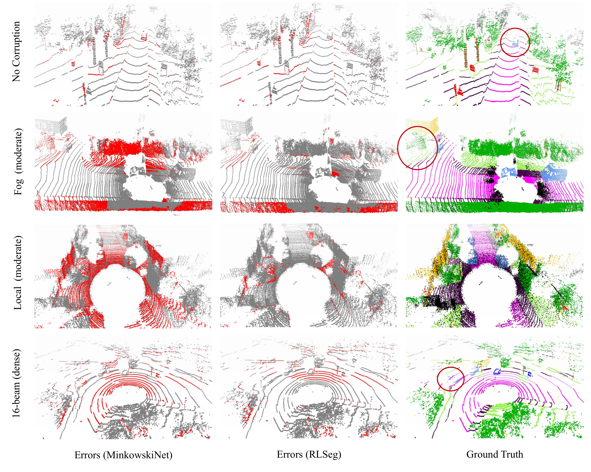
Visualization. We provide visualization results of our RLSeg and teacher MinkowskiNet in Fig. 15, in which our proposed model performs better. Specifically, MinkowskiNet cannot work normally in fog simulation and local distortion, and there are large areas of errors in the LiDAR scenes. In contrast, our RLSeg provides robust prediction even for the small objects (as shown in red circles). These show the robustness of our model as well as the promising future for robust LIDAR semantic segmentation.
Ablation study. We analyze different designs through an ablation study on SemanticKITTI-C. As shown in Tab. 8, exploiting our architecture improves the robustness to 81.3%, but causes a performance drop to 63.3 mIoU. After using Mix3D, there is a huge performance boost from 63.3 to 67.0 mIoU, while increasing the robustness from 81.3% to 84.7%. Although knowledge distillation (KD) does not improve the robustness significantly, it boost the performance on clean data from 67.0 to 70.9. Finally, utilizing pseudo label fine-tuning can further improve the performance while keeping the robustness, which shows a promising improvement by leveraging the potential of semi-supervised learning, giving a performance boost to about 73.5%. This also gives hints for future work that improve the robust but poor performance network to better performance.
7 Conclusion
In this paper, we propose new benchmarks called SemanticKITTI-C and SemanticPOSS-C, with respect to real-world and out-of-domain LiDAR corruptions. We systematically investigate a wide range of LiDAR semantic segmentation models, spanning different input representations and network architectures. After analyzing the results of previous approaches, we summarized 12 observations for the future research. Finally, we propose RLSeg based on the above observations, which effectively boosts the robustness of LiDAR semantic segmentation. We hope our benchmark, comprehensive analysis and observations could boost future research for robust LiDAR semantic segmentation in safety-critical applications.
Declarations
Supplementary information
Our dataset and code will be available at https://yanx27.github.io/RobustLidarSeg/.
Funding
This work was supported in part by the Basic Research Project No. HZQB-KCZYZ-2021067 of Hetao Shenzhen HK S&T Cooperation Zone, by the National Key R&D Program of China with grant No.2018YFB1800800, by Shenzhen Outstanding Talents Training Fund, by Guangdong Research Project No. 2017ZT07X152 and No. 2019CX01X104, by the Guangdong Provincial Key Laboratory of Future Networks of Intelligence (Grant No. 2022B1212010001), by the NSFC 61931024&8192 2046, by NSFC-Youth 62106154&62302399, by zelixir biotechnology company Fund, by Tencent Open Fund, and by ITSO at CUHKSZ.
Competing interests
The authors have no competing interests to declare that are relevant to the content of this article.
Availability of data and materials
All the datasets used in the paper are publicly available.
Authors’ contributions
X. Yan and D. Dai conceptualized the work and designed the methodology. X. Yan and C. Zheng formulated the mathematical formulation. X. Yan conducted the experiments on SemanticKITTI-C and Y. Xue conducted the experiments on SemanticPOSS-C. X. Yan, D. Dai, and Z. Li analyzed the results. D. Dai, Z. Li and S. Cui supervised the work. All authors wrote and revised the manuscript.
References
- Alonso \BOthers. (\APACyear2020) \APACinsertmetastaralonso20203d{APACrefauthors}Alonso, I., Riazuelo, L., Montesano, L.\BCBL Murillo, A.C. \APACrefYearMonthDay2020. \BBOQ\APACrefatitle3D-MiniNet: Learning a 2D Representation from Point Clouds for Fast and Efficient 3D LIDAR Semantic Segmentation 3d-mininet: Learning a 2d representation from point clouds for fast and efficient 3d lidar semantic segmentation.\BBCQ \APACjournalVolNumPagesarXiv preprint arXiv:2002.10893. \PrintBackRefs\CurrentBib
- Altindis \BOthers. (\APACyear2021) \APACinsertmetastaraltindis2021benchmarking{APACrefauthors}Altindis, S.F., Dalva, Y.\BCBL Dundar, A. \APACrefYearMonthDay2021. \BBOQ\APACrefatitleBenchmarking the Robustness of Instance Segmentation Models Benchmarking the robustness of instance segmentation models.\BBCQ \APACjournalVolNumPagesarXiv preprint arXiv:2109.01123. \PrintBackRefs\CurrentBib
- Bai \BOthers. (\APACyear2022) \APACinsertmetastarbai2022transfusion{APACrefauthors}Bai, X., Hu, Z., Zhu, X., Huang, Q., Chen, Y., Fu, H.\BCBL Tai, C\BHBIL. \APACrefYearMonthDay2022. \BBOQ\APACrefatitleTransfusion: Robust lidar-camera fusion for 3d object detection with transformers Transfusion: Robust lidar-camera fusion for 3d object detection with transformers.\BBCQ \APACrefbtitleProceedings of the IEEE/CVF Conference on Computer Vision and Pattern Recognition Proceedings of the ieee/cvf conference on computer vision and pattern recognition (\BPGS 1090–1099). \PrintBackRefs\CurrentBib
- Barbu \BOthers. (\APACyear2019) \APACinsertmetastarbarbu2019objectnet{APACrefauthors}Barbu, A., Mayo, D., Alverio, J., Luo, W., Wang, C., Gutfreund, D.\BDBLKatz, B. \APACrefYearMonthDay2019. \BBOQ\APACrefatitleObjectnet: A large-scale bias-controlled dataset for pushing the limits of object recognition models Objectnet: A large-scale bias-controlled dataset for pushing the limits of object recognition models.\BBCQ \APACjournalVolNumPagesAdvances in neural information processing systems32. \PrintBackRefs\CurrentBib
- Behley \BOthers. (\APACyear2019) \APACinsertmetastarbehley2019semantickitti{APACrefauthors}Behley, J., Garbade, M., Milioto, A., Quenzel, J., Behnke, S., Stachniss, C.\BCBL Gall, J. \APACrefYearMonthDay2019. \BBOQ\APACrefatitleSemanticKITTI: A dataset for semantic scene understanding of lidar sequences Semantickitti: A dataset for semantic scene understanding of lidar sequences.\BBCQ \APACrefbtitleProceedings of the IEEE International Conference on Computer Vision Proceedings of the ieee international conference on computer vision (\BPGS 9297–9307). \PrintBackRefs\CurrentBib
- Caesar \BOthers. (\APACyear2020) \APACinsertmetastarcaesar2020nuscenes{APACrefauthors}Caesar, H., Bankiti, V., Lang, A.H., Vora, S., Liong, V.E., Xu, Q.\BDBLBeijbom, O. \APACrefYearMonthDay2020. \BBOQ\APACrefatitlenuscenes: A multimodal dataset for autonomous driving nuscenes: A multimodal dataset for autonomous driving.\BBCQ \APACrefbtitleProceedings of the IEEE/CVF conference on computer vision and pattern recognition Proceedings of the ieee/cvf conference on computer vision and pattern recognition (\BPGS 11621–11631). \PrintBackRefs\CurrentBib
- H\BHBIX. Cheng \BOthers. (\APACyear2022) \APACinsertmetastarcheng2022cenet{APACrefauthors}Cheng, H\BHBIX., Han, X\BHBIF.\BCBL Xiao, G\BHBIQ. \APACrefYearMonthDay2022. \BBOQ\APACrefatitleCenet: Toward Concise and Efficient Lidar Semantic Segmentation for Autonomous Driving Cenet: Toward concise and efficient lidar semantic segmentation for autonomous driving.\BBCQ \APACrefbtitle2022 IEEE International Conference on Multimedia and Expo (ICME) 2022 ieee international conference on multimedia and expo (icme) (\BPGS 01–06). \PrintBackRefs\CurrentBib
- R. Cheng \BOthers. (\APACyear2021) \APACinsertmetastarcheng20212{APACrefauthors}Cheng, R., Razani, R., Taghavi, E., Li, E.\BCBL Liu, B. \APACrefYearMonthDay2021. \BBOQ\APACrefatitleAf2-s3net: Attentive feature fusion with adaptive feature selection for sparse semantic segmentation network Af2-s3net: Attentive feature fusion with adaptive feature selection for sparse semantic segmentation network.\BBCQ \APACrefbtitleProceedings of the IEEE/CVF conference on computer vision and pattern recognition Proceedings of the ieee/cvf conference on computer vision and pattern recognition (\BPGS 12547–12556). \PrintBackRefs\CurrentBib
- Choy \BOthers. (\APACyear2019) \APACinsertmetastarchoy20194d{APACrefauthors}Choy, C., Gwak, J.\BCBL Savarese, S. \APACrefYearMonthDay2019. \BBOQ\APACrefatitle4D Spatio-Temporal ConvNets: Minkowski Convolutional Neural Networks 4d spatio-temporal convnets: Minkowski convolutional neural networks.\BBCQ \APACrefbtitleProceedings of the IEEE Conference on Computer Vision and Pattern Recognition Proceedings of the ieee conference on computer vision and pattern recognition (\BPGS 3075–3084). \PrintBackRefs\CurrentBib
- Cordts \BOthers. (\APACyear2016) \APACinsertmetastarCordts2016Cityscapes{APACrefauthors}Cordts, M., Omran, M., Ramos, S., Rehfeld, T., Enzweiler, M., Benenson, R.\BDBLSchiele, B. \APACrefYearMonthDay2016. \BBOQ\APACrefatitleThe Cityscapes Dataset for Semantic Urban Scene Understanding The cityscapes dataset for semantic urban scene understanding.\BBCQ \APACrefbtitleProc. of the IEEE Conference on Computer Vision and Pattern Recognition (CVPR). Proc. of the ieee conference on computer vision and pattern recognition (cvpr). \PrintBackRefs\CurrentBib
- Cortinhal \BOthers. (\APACyear2020) \APACinsertmetastarcortinhal2020salsanext{APACrefauthors}Cortinhal, T., Tzelepis, G.\BCBL Aksoy, E.E. \APACrefYearMonthDay2020. \BBOQ\APACrefatitleSalsanext: Fast, uncertainty-aware semantic segmentation of lidar point clouds for autonomous driving Salsanext: Fast, uncertainty-aware semantic segmentation of lidar point clouds for autonomous driving.\BBCQ \APACjournalVolNumPagesarXiv preprint arXiv:2003.03653. \PrintBackRefs\CurrentBib
- Deng \BOthers. (\APACyear2009) \APACinsertmetastardeng2009imagenet{APACrefauthors}Deng, J., Dong, W., Socher, R., Li, L\BHBIJ., Li, K.\BCBL Fei-Fei, L. \APACrefYearMonthDay2009. \BBOQ\APACrefatitleImagenet: A large-scale hierarchical image database Imagenet: A large-scale hierarchical image database.\BBCQ \APACrefbtitle2009 IEEE conference on computer vision and pattern recognition 2009 ieee conference on computer vision and pattern recognition (\BPGS 248–255). \PrintBackRefs\CurrentBib
- Dong \BOthers. (\APACyear2020) \APACinsertmetastardong2020self{APACrefauthors}Dong, X., Chen, D., Zhou, H., Hua, G., Zhang, W.\BCBL Yu, N. \APACrefYearMonthDay2020. \BBOQ\APACrefatitleSelf-robust 3d point recognition via gather-vector guidance Self-robust 3d point recognition via gather-vector guidance.\BBCQ \APACrefbtitle2020 IEEE/CVF Conference on Computer Vision and Pattern Recognition (CVPR) 2020 ieee/cvf conference on computer vision and pattern recognition (cvpr) (\BPGS 11513–11521). \PrintBackRefs\CurrentBib
- Engel \BOthers. (\APACyear2021) \APACinsertmetastarengel2021point{APACrefauthors}Engel, N., Belagiannis, V.\BCBL Dietmayer, K. \APACrefYearMonthDay2021. \BBOQ\APACrefatitlePoint transformer Point transformer.\BBCQ \APACjournalVolNumPagesIEEE Access9134826–134840. \PrintBackRefs\CurrentBib
- Geiger \BOthers. (\APACyear2012) \APACinsertmetastargeiger2012cvpr{APACrefauthors}Geiger, A., Lenz, P.\BCBL Urtasun, R. \APACrefYearMonthDay2012. \BBOQ\APACrefatitleAre we ready for Autonomous Driving? The KITTI Vision Benchmark Suite Are we ready for Autonomous Driving? The KITTI Vision Benchmark Suite.\BBCQ \APACrefbtitleProc. of the IEEE Conf. on Computer Vision and Pattern Recognition (CVPR) Proc. of the ieee conf. on computer vision and pattern recognition (cvpr) (\BPGS 3354–3361). \PrintBackRefs\CurrentBib
- Graham \BOthers. (\APACyear2018) \APACinsertmetastarSparseConv{APACrefauthors}Graham, B., Engelcke, M.\BCBL van der Maaten, L. \APACrefYearMonthDay2018. \BBOQ\APACrefatitle3d semantic segmentation with submanifold sparse convolutional networks 3d semantic segmentation with submanifold sparse convolutional networks.\BBCQ \APACrefbtitleProceedings of the IEEE Conference on Computer Vision and Pattern Recognition Proceedings of the ieee conference on computer vision and pattern recognition (\BPGS 9224–9232). \PrintBackRefs\CurrentBib
- Graham \BBA van der Maaten (\APACyear2017) \APACinsertmetastargraham2017submanifold{APACrefauthors}Graham, B.\BCBT \BBA van der Maaten, L. \APACrefYearMonthDay2017. \BBOQ\APACrefatitleSubmanifold sparse convolutional networks Submanifold sparse convolutional networks.\BBCQ \APACjournalVolNumPagesarXiv preprint arXiv:1706.01307. \PrintBackRefs\CurrentBib
- Hahner \BOthers. (\APACyear2019) \APACinsertmetastarFoggySynscapes{APACrefauthors}Hahner, M., Dai, D., Sakaridis, C., Zaech, J\BHBIN.\BCBL Van Gool, L. \APACrefYearMonthDay2019. \BBOQ\APACrefatitleSemantic Understanding of Foggy Scenes with Purely Synthetic Data Semantic understanding of foggy scenes with purely synthetic data.\BBCQ \APACrefbtitleIEEE International Conference on Intelligent Transportation Systems (ITSC). Ieee international conference on intelligent transportation systems (itsc). \PrintBackRefs\CurrentBib
- Hahner \BOthers. (\APACyear2022\APACexlab\BCnt1) \APACinsertmetastarHahnerCVPR22{APACrefauthors}Hahner, M., Sakaridis, C., Bijelic, M., Heide, F., Yu, F., Dai, D.\BCBL Van Gool, L. \APACrefYearMonthDay2022\BCnt1. \BBOQ\APACrefatitleLiDAR Snowfall Simulation for Robust 3D Object Detection LiDAR Snowfall Simulation for Robust 3D Object Detection.\BBCQ \APACrefbtitleIEEE/CVF Conference on Computer Vision and Pattern Recognition (CVPR). Ieee/cvf conference on computer vision and pattern recognition (cvpr). \PrintBackRefs\CurrentBib
- Hahner \BOthers. (\APACyear2022\APACexlab\BCnt2) \APACinsertmetastarhahner2022lidar{APACrefauthors}Hahner, M., Sakaridis, C., Bijelic, M., Heide, F., Yu, F., Dai, D.\BCBL Van Gool, L. \APACrefYearMonthDay2022\BCnt2. \BBOQ\APACrefatitleLidar snowfall simulation for robust 3d object detection Lidar snowfall simulation for robust 3d object detection.\BBCQ \APACrefbtitleProceedings of the IEEE/CVF Conference on Computer Vision and Pattern Recognition Proceedings of the ieee/cvf conference on computer vision and pattern recognition (\BPGS 16364–16374). \PrintBackRefs\CurrentBib
- Hahner \BOthers. (\APACyear2021) \APACinsertmetastarhahner2021fog{APACrefauthors}Hahner, M., Sakaridis, C., Dai, D.\BCBL Van Gool, L. \APACrefYearMonthDay2021. \BBOQ\APACrefatitleFog simulation on real LiDAR point clouds for 3D object detection in adverse weather Fog simulation on real lidar point clouds for 3d object detection in adverse weather.\BBCQ \APACrefbtitleProceedings of the IEEE/CVF International Conference on Computer Vision Proceedings of the ieee/cvf international conference on computer vision (\BPGS 15283–15292). \PrintBackRefs\CurrentBib
- Hendrycks \BBA Dietterich (\APACyear2019) \APACinsertmetastarhendrycks2019benchmarking{APACrefauthors}Hendrycks, D.\BCBT \BBA Dietterich, T. \APACrefYearMonthDay2019. \BBOQ\APACrefatitleBenchmarking neural network robustness to common corruptions and perturbations Benchmarking neural network robustness to common corruptions and perturbations.\BBCQ \APACjournalVolNumPagesarXiv preprint arXiv:1903.12261. \PrintBackRefs\CurrentBib
- Hendrycks \BOthers. (\APACyear2021) \APACinsertmetastarhendrycks2021natural{APACrefauthors}Hendrycks, D., Zhao, K., Basart, S., Steinhardt, J.\BCBL Song, D. \APACrefYearMonthDay2021. \BBOQ\APACrefatitleNatural adversarial examples Natural adversarial examples.\BBCQ \APACrefbtitleProceedings of the IEEE/CVF Conference on Computer Vision and Pattern Recognition Proceedings of the ieee/cvf conference on computer vision and pattern recognition (\BPGS 15262–15271). \PrintBackRefs\CurrentBib
- Hinton \BOthers. (\APACyear2014) \APACinsertmetastarhinton2015distilling{APACrefauthors}Hinton, G., Vinyals, O.\BCBL Dean, J. \APACrefYearMonthDay2014. \BBOQ\APACrefatitleDistilling the knowledge in a neural network Distilling the knowledge in a neural network.\BBCQ \APACjournalVolNumPagesNeurIPS Workshops. \PrintBackRefs\CurrentBib
- Hu \BOthers. (\APACyear2022) \APACinsertmetastarhu2022sensaturban{APACrefauthors}Hu, Q., Yang, B., Khalid, S., Xiao, W., Trigoni, N.\BCBL Markham, A. \APACrefYearMonthDay2022. \BBOQ\APACrefatitleSensaturban: Learning semantics from urban-scale photogrammetric point clouds Sensaturban: Learning semantics from urban-scale photogrammetric point clouds.\BBCQ \APACjournalVolNumPagesInternational Journal of Computer Vision1302316–343. \PrintBackRefs\CurrentBib
- Hu \BOthers. (\APACyear2020) \APACinsertmetastarhu2019randla{APACrefauthors}Hu, Q., Yang, B., Xie, L., Rosa, S., Guo, Y., Wang, Z.\BDBLMarkham, A. \APACrefYearMonthDay2020. \BBOQ\APACrefatitleRandLA-Net: Efficient Semantic Segmentation of Large-Scale Point Clouds Randla-net: Efficient semantic segmentation of large-scale point clouds.\BBCQ \APACjournalVolNumPagesProceedings of the IEEE Conference on Computer Vision and Pattern Recognition. \PrintBackRefs\CurrentBib
- Hua \BOthers. (\APACyear2018) \APACinsertmetastarhua2018pointwise{APACrefauthors}Hua, B\BHBIS., Tran, M\BHBIK.\BCBL Yeung, S\BHBIK. \APACrefYearMonthDay2018. \BBOQ\APACrefatitlePointwise convolutional neural networks Pointwise convolutional neural networks.\BBCQ \APACrefbtitleProceedings of the IEEE Conference on Computer Vision and Pattern Recognition Proceedings of the ieee conference on computer vision and pattern recognition (\BPGS 984–993). \PrintBackRefs\CurrentBib
- Kamann \BBA Rother (\APACyear2020) \APACinsertmetastarkamann2020benchmarking{APACrefauthors}Kamann, C.\BCBT \BBA Rother, C. \APACrefYearMonthDay2020. \BBOQ\APACrefatitleBenchmarking the robustness of semantic segmentation models Benchmarking the robustness of semantic segmentation models.\BBCQ \APACrefbtitleProceedings of the IEEE/CVF Conference on Computer Vision and Pattern Recognition Proceedings of the ieee/cvf conference on computer vision and pattern recognition (\BPGS 8828–8838). \PrintBackRefs\CurrentBib
- Kong \BOthers. (\APACyear2022) \APACinsertmetastarkong2022lasermix{APACrefauthors}Kong, L., Ren, J., Pan, L.\BCBL Liu, Z. \APACrefYearMonthDay2022. \BBOQ\APACrefatitleLaserMix for Semi-Supervised LiDAR Semantic Segmentation Lasermix for semi-supervised lidar semantic segmentation.\BBCQ \APACjournalVolNumPagesarXiv preprint arXiv:2207.00026. \PrintBackRefs\CurrentBib
- Lai \BOthers. (\APACyear2022) \APACinsertmetastarlai2022stratified{APACrefauthors}Lai, X., Liu, J., Jiang, L., Wang, L., Zhao, H., Liu, S.\BDBLJia, J. \APACrefYearMonthDay2022. \BBOQ\APACrefatitleStratified Transformer for 3D Point Cloud Segmentation Stratified transformer for 3d point cloud segmentation.\BBCQ \APACrefbtitleProceedings of the IEEE/CVF Conference on Computer Vision and Pattern Recognition Proceedings of the ieee/cvf conference on computer vision and pattern recognition (\BPGS 8500–8509). \PrintBackRefs\CurrentBib
- J. Li \BOthers. (\APACyear2022) \APACinsertmetastarsdseg3d_eccv2022{APACrefauthors}Li, J., Dai, H.\BCBL Ding, Y. \APACrefYearMonthDay2022. \BBOQ\APACrefatitleSelf-Distillation for Robust LiDAR Semantic Segmentation in Autonomous Driving Self-distillation for robust LiDAR semantic segmentation in autonomous driving.\BBCQ \APACrefbtitleECCV. Eccv. \PrintBackRefs\CurrentBib
- Y. Li \BOthers. (\APACyear2022) \APACinsertmetastarli2022deepfusion{APACrefauthors}Li, Y., Yu, A.W., Meng, T., Caine, B., Ngiam, J., Peng, D.\BDBLothers \APACrefYearMonthDay2022. \BBOQ\APACrefatitleDeepfusion: Lidar-camera deep fusion for multi-modal 3d object detection Deepfusion: Lidar-camera deep fusion for multi-modal 3d object detection.\BBCQ \APACrefbtitleProceedings of the IEEE/CVF Conference on Computer Vision and Pattern Recognition Proceedings of the ieee/cvf conference on computer vision and pattern recognition (\BPGS 17182–17191). \PrintBackRefs\CurrentBib
- Liong \BOthers. (\APACyear2020) \APACinsertmetastarliong2020amvnet{APACrefauthors}Liong, V.E., Nguyen, T.N.T., Widjaja, S., Sharma, D.\BCBL Chong, Z.J. \APACrefYearMonthDay2020. \BBOQ\APACrefatitleAmvnet: Assertion-based multi-view fusion network for lidar semantic segmentation Amvnet: Assertion-based multi-view fusion network for lidar semantic segmentation.\BBCQ \APACjournalVolNumPagesarXiv preprint arXiv:2012.04934. \PrintBackRefs\CurrentBib
- H. Liu \BOthers. (\APACyear2021) \APACinsertmetastarliu2021pointguard{APACrefauthors}Liu, H., Jia, J.\BCBL Gong, N.Z. \APACrefYearMonthDay2021. \BBOQ\APACrefatitlePointguard: Provably robust 3d point cloud classification Pointguard: Provably robust 3d point cloud classification.\BBCQ \APACrefbtitleProceedings of the IEEE/CVF Conference on Computer Vision and Pattern Recognition Proceedings of the ieee/cvf conference on computer vision and pattern recognition (\BPGS 6186–6195). \PrintBackRefs\CurrentBib
- Y. Liu \BOthers. (\APACyear2019) \APACinsertmetastarliu2019relation{APACrefauthors}Liu, Y., Fan, B., Xiang, S.\BCBL Pan, C. \APACrefYearMonthDay2019. \BBOQ\APACrefatitleRelation-shape convolutional neural network for point cloud analysis Relation-shape convolutional neural network for point cloud analysis.\BBCQ \APACrefbtitleProceedings of the IEEE/CVF Conference on Computer Vision and Pattern Recognition Proceedings of the ieee/cvf conference on computer vision and pattern recognition (\BPGS 8895–8904). \PrintBackRefs\CurrentBib
- Michaelis \BOthers. (\APACyear2019) \APACinsertmetastarmichaelis2019benchmarking{APACrefauthors}Michaelis, C., Mitzkus, B., Geirhos, R., Rusak, E., Bringmann, O., Ecker, A.S.\BDBLBrendel, W. \APACrefYearMonthDay2019. \BBOQ\APACrefatitleBenchmarking robustness in object detection: Autonomous driving when winter is coming Benchmarking robustness in object detection: Autonomous driving when winter is coming.\BBCQ \APACjournalVolNumPagesarXiv preprint arXiv:1907.07484. \PrintBackRefs\CurrentBib
- Milioto \BOthers. (\APACyear2019) \APACinsertmetastarmilioto2019rangenet++{APACrefauthors}Milioto, A., Vizzo, I., Behley, J.\BCBL Stachniss, C. \APACrefYearMonthDay2019. \BBOQ\APACrefatitleRangenet++: Fast and accurate lidar semantic segmentation Rangenet++: Fast and accurate lidar semantic segmentation.\BBCQ \APACrefbtitleProc. of the IEEE/RSJ Intl. Conf. on Intelligent Robots and Systems (IROS). Proc. of the ieee/rsj intl. conf. on intelligent robots and systems (iros). \PrintBackRefs\CurrentBib
- Nekrasov \BOthers. (\APACyear2021) \APACinsertmetastarNekrasov213DV{APACrefauthors}Nekrasov, A., Schult, J., Litany, O., Leibe, B.\BCBL Engelmann, F. \APACrefYearMonthDay2021. \BBOQ\APACrefatitleMix3D: Out-of-Context Data Augmentation for 3D Scenes Mix3D: Out-of-Context Data Augmentation for 3D Scenes.\BBCQ \APACrefbtitleInternational Conference on 3D Vision (3DV). International Conference on 3D Vision (3DV). \PrintBackRefs\CurrentBib
- Pan \BOthers. (\APACyear2020) \APACinsertmetastarpan2020semanticposs{APACrefauthors}Pan, Y., Gao, B., Mei, J., Geng, S., Li, C.\BCBL Zhao, H. \APACrefYearMonthDay2020. \BBOQ\APACrefatitleSemanticPOSS: A Point Cloud Dataset with Large Quantity of Dynamic Instances Semanticposs: A point cloud dataset with large quantity of dynamic instances.\BBCQ \APACjournalVolNumPagesarXiv preprint arXiv:2002.09147. \PrintBackRefs\CurrentBib
- Porav \BOthers. (\APACyear2020) \APACinsertmetastarporav2020rainy{APACrefauthors}Porav, H., Musat, V\BHBIN., Bruls, T.\BCBL Newman, P. \APACrefYearMonthDay2020. \BBOQ\APACrefatitleRainy screens: Collecting rainy datasets, indoors Rainy screens: Collecting rainy datasets, indoors.\BBCQ \APACjournalVolNumPagesarXiv preprint arXiv:2003.04742. \PrintBackRefs\CurrentBib
- Qi \BOthers. (\APACyear2017) \APACinsertmetastarqi2017pointnet++{APACrefauthors}Qi, C.R., Yi, L., Su, H.\BCBL Guibas, L.J. \APACrefYearMonthDay2017. \BBOQ\APACrefatitlePointnet++: Deep hierarchical feature learning on point sets in a metric space Pointnet++: Deep hierarchical feature learning on point sets in a metric space.\BBCQ \APACrefbtitleAdvances in neural information processing systems Advances in neural information processing systems (\BPGS 5099–5108). \PrintBackRefs\CurrentBib
- Qiu \BOthers. (\APACyear2022) \APACinsertmetastarqiu2022gfnet{APACrefauthors}Qiu, H., Yu, B.\BCBL Tao, D. \APACrefYearMonthDay2022. \BBOQ\APACrefatitleGFNet: Geometric Flow Network for 3D Point Cloud Semantic Segmentation GFNet: Geometric flow network for 3d point cloud semantic segmentation.\BBCQ \APACjournalVolNumPagesTransactions on Machine Learning Research. {APACrefURL} https://openreview.net/forum?id=LSAAlS7Yts \PrintBackRefs\CurrentBib
- Recht \BOthers. (\APACyear2019) \APACinsertmetastarrecht2019imagenet{APACrefauthors}Recht, B., Roelofs, R., Schmidt, L.\BCBL Shankar, V. \APACrefYearMonthDay2019. \BBOQ\APACrefatitleDo imagenet classifiers generalize to imagenet? Do imagenet classifiers generalize to imagenet?\BBCQ \APACrefbtitleInternational Conference on Machine Learning International conference on machine learning (\BPGS 5389–5400). \PrintBackRefs\CurrentBib
- Ren \BOthers. (\APACyear2022) \APACinsertmetastarren2022modelnet-c{APACrefauthors}Ren, J., Pan, L.\BCBL Liu, Z. \APACrefYearMonthDay2022. \BBOQ\APACrefatitleBenchmarking and Analyzing Point Cloud Classification under Corruptions Benchmarking and analyzing point cloud classification under corruptions.\BBCQ \APACjournalVolNumPagesInternational Conference on Machine Learning (ICML). \PrintBackRefs\CurrentBib
- Ronneberger \BOthers. (\APACyear2015) \APACinsertmetastarronneberger2015u{APACrefauthors}Ronneberger, O., Fischer, P.\BCBL Brox, T. \APACrefYearMonthDay2015. \BBOQ\APACrefatitleU-net: Convolutional networks for biomedical image segmentation U-net: Convolutional networks for biomedical image segmentation.\BBCQ \APACrefbtitleInternational Conference on Medical image computing and computer-assisted intervention International conference on medical image computing and computer-assisted intervention (\BPGS 234–241). \PrintBackRefs\CurrentBib
- Sakaridis \BOthers. (\APACyear2018) \APACinsertmetastarsakaridis2018semantic{APACrefauthors}Sakaridis, C., Dai, D.\BCBL Van Gool, L. \APACrefYearMonthDay2018. \BBOQ\APACrefatitleSemantic foggy scene understanding with synthetic data Semantic foggy scene understanding with synthetic data.\BBCQ \APACjournalVolNumPagesInternational Journal of Computer Vision1269973–992. \PrintBackRefs\CurrentBib
- Sakaridis \BOthers. (\APACyear2021) \APACinsertmetastarsakaridis2021acdc{APACrefauthors}Sakaridis, C., Dai, D.\BCBL Van Gool, L. \APACrefYearMonthDay2021. \BBOQ\APACrefatitleACDC: The adverse conditions dataset with correspondences for semantic driving scene understanding Acdc: The adverse conditions dataset with correspondences for semantic driving scene understanding.\BBCQ \APACrefbtitleProceedings of the IEEE/CVF International Conference on Computer Vision Proceedings of the ieee/cvf international conference on computer vision (\BPGS 10765–10775). \PrintBackRefs\CurrentBib
- Sun \BOthers. (\APACyear2020) \APACinsertmetastarsun2020scalability{APACrefauthors}Sun, P., Kretzschmar, H., Dotiwalla, X., Chouard, A., Patnaik, V., Tsui, P.\BDBLothers \APACrefYearMonthDay2020. \BBOQ\APACrefatitleScalability in perception for autonomous driving: Waymo open dataset Scalability in perception for autonomous driving: Waymo open dataset.\BBCQ \APACrefbtitleProceedings of the IEEE/CVF conference on computer vision and pattern recognition Proceedings of the ieee/cvf conference on computer vision and pattern recognition (\BPGS 2446–2454). \PrintBackRefs\CurrentBib
- Taghanaki \BOthers. (\APACyear2020) \APACinsertmetastartaghanaki2020robustpointset{APACrefauthors}Taghanaki, S.A., Luo, J., Zhang, R., Wang, Y., Jayaraman, P.K.\BCBL Jatavallabhula, K.M. \APACrefYearMonthDay2020. \BBOQ\APACrefatitleRobustpointset: A dataset for benchmarking robustness of point cloud classifiers Robustpointset: A dataset for benchmarking robustness of point cloud classifiers.\BBCQ \APACjournalVolNumPagesarXiv preprint arXiv:2011.11572. \PrintBackRefs\CurrentBib
- Tang \BOthers. (\APACyear2020) \APACinsertmetastartang2020searching{APACrefauthors}Tang, H., Liu, Z., Zhao, S., Lin, Y., Lin, J., Wang, H.\BCBL Han, S. \APACrefYearMonthDay2020. \BBOQ\APACrefatitleSearching efficient 3d architectures with sparse point-voxel convolution Searching efficient 3d architectures with sparse point-voxel convolution.\BBCQ \APACrefbtitleEuropean conference on computer vision European conference on computer vision (\BPGS 685–702). \PrintBackRefs\CurrentBib
- Tatarchenko \BOthers. (\APACyear2018) \APACinsertmetastartatarchenko2018tangent{APACrefauthors}Tatarchenko, M., Park, J., Koltun, V.\BCBL Zhou, Q\BHBIY. \APACrefYearMonthDay2018. \BBOQ\APACrefatitleTangent convolutions for dense prediction in 3d Tangent convolutions for dense prediction in 3d.\BBCQ \APACrefbtitleProceedings of the IEEE Conference on Computer Vision and Pattern Recognition Proceedings of the ieee conference on computer vision and pattern recognition (\BPGS 3887–3896). \PrintBackRefs\CurrentBib
- Thomas \BOthers. (\APACyear2019) \APACinsertmetastarThomas_2019_ICCV{APACrefauthors}Thomas, H., Qi, C.R., Deschaud, J\BHBIE., Marcotegui, B., Goulette, F.\BCBL Guibas, L.J. \APACrefYearMonthDay2019October. \BBOQ\APACrefatitleKPConv: Flexible and Deformable Convolution for Point Clouds Kpconv: Flexible and deformable convolution for point clouds.\BBCQ \APACrefbtitleThe IEEE International Conference on Computer Vision (ICCV). The ieee international conference on computer vision (iccv). \PrintBackRefs\CurrentBib
- Unal \BOthers. (\APACyear2022) \APACinsertmetastarUnal_2022_CVPR{APACrefauthors}Unal, O., Dai, D.\BCBL Van Gool, L. \APACrefYearMonthDay2022. \BBOQ\APACrefatitleScribble-Supervised LiDAR Semantic Segmentation Scribble-supervised lidar semantic segmentation.\BBCQ \APACrefbtitleProceedings of the IEEE/CVF Conference on Computer Vision and Pattern Recognition (CVPR). Proceedings of the ieee/cvf conference on computer vision and pattern recognition (cvpr). \PrintBackRefs\CurrentBib
- Vaswani \BOthers. (\APACyear2017) \APACinsertmetastarvaswani2017attention{APACrefauthors}Vaswani, A., Shazeer, N., Parmar, N., Uszkoreit, J., Jones, L., Gomez, A.N.\BDBLPolosukhin, I. \APACrefYearMonthDay2017. \BBOQ\APACrefatitleAttention is all you need Attention is all you need.\BBCQ \APACrefbtitleAdvances in neural information processing systems Advances in neural information processing systems (\BPGS 5998–6008). \PrintBackRefs\CurrentBib
- Wang \BOthers. (\APACyear2019) \APACinsertmetastarwang2019dynamic{APACrefauthors}Wang, Y., Sun, Y., Liu, Z., Sarma, S.E., Bronstein, M.M.\BCBL Solomon, J.M. \APACrefYearMonthDay2019. \BBOQ\APACrefatitleDynamic graph cnn for learning on point clouds Dynamic graph cnn for learning on point clouds.\BBCQ \APACjournalVolNumPagesACM Transactions on Graphics (TOG)3851–12. \PrintBackRefs\CurrentBib
- Wei \BOthers. (\APACyear2022) \APACinsertmetastarwei2022lidar{APACrefauthors}Wei, Y., Wei, Z., Rao, Y., Li, J., Zhou, J.\BCBL Lu, J. \APACrefYearMonthDay2022. \BBOQ\APACrefatitleLiDAR Distillation: Bridging the Beam-Induced Domain Gap for 3D Object Detection Lidar distillation: Bridging the beam-induced domain gap for 3d object detection.\BBCQ \APACrefbtitleEuropean Conference on Computer Vision (ECCV) European conference on computer vision (eccv) (\BVOL 39, \BPG 179-195). \PrintBackRefs\CurrentBib
- B. Wu \BOthers. (\APACyear2018) \APACinsertmetastarwu2018squeezeseg{APACrefauthors}Wu, B., Wan, A., Yue, X.\BCBL Keutzer, K. \APACrefYearMonthDay2018. \BBOQ\APACrefatitleSqueezeseg: Convolutional neural nets with recurrent crf for real-time road-object segmentation from 3d lidar point cloud Squeezeseg: Convolutional neural nets with recurrent crf for real-time road-object segmentation from 3d lidar point cloud.\BBCQ \APACrefbtitle2018 IEEE International Conference on Robotics and Automation (ICRA) 2018 ieee international conference on robotics and automation (icra) (\BPGS 1887–1893). \PrintBackRefs\CurrentBib
- B. Wu \BOthers. (\APACyear2019) \APACinsertmetastarwu2019squeezesegv2{APACrefauthors}Wu, B., Zhou, X., Zhao, S., Yue, X.\BCBL Keutzer, K. \APACrefYearMonthDay2019. \BBOQ\APACrefatitleSqueezesegv2: Improved model structure and unsupervised domain adaptation for road-object segmentation from a lidar point cloud Squeezesegv2: Improved model structure and unsupervised domain adaptation for road-object segmentation from a lidar point cloud.\BBCQ \APACrefbtitle2019 International Conference on Robotics and Automation (ICRA) 2019 international conference on robotics and automation (icra) (\BPGS 4376–4382). \PrintBackRefs\CurrentBib
- W. Wu \BOthers. (\APACyear2019) \APACinsertmetastarPointConv{APACrefauthors}Wu, W., Qi, Z.\BCBL Fuxin, L. \APACrefYearMonthDay2019. \BBOQ\APACrefatitlePointconv: Deep convolutional networks on 3d point clouds Pointconv: Deep convolutional networks on 3d point clouds.\BBCQ \APACrefbtitleProceedings of the IEEE Conference on Computer Vision and Pattern Recognition Proceedings of the ieee conference on computer vision and pattern recognition (\BPGS 9621–9630). \PrintBackRefs\CurrentBib
- Xiao \BBA Wachs (\APACyear2021) \APACinsertmetastarxiao2021triangle{APACrefauthors}Xiao, C.\BCBT \BBA Wachs, J. \APACrefYearMonthDay2021. \BBOQ\APACrefatitleTriangle-net: Towards robustness in point cloud learning Triangle-net: Towards robustness in point cloud learning.\BBCQ \APACrefbtitleProceedings of the IEEE/CVF Winter Conference on Applications of Computer Vision Proceedings of the ieee/cvf winter conference on applications of computer vision (\BPGS 826–835). \PrintBackRefs\CurrentBib
- Xu \BOthers. (\APACyear2021) \APACinsertmetastarxu2021rpvnet{APACrefauthors}Xu, J., Zhang, R., Dou, J., Zhu, Y., Sun, J.\BCBL Pu, S. \APACrefYearMonthDay2021. \BBOQ\APACrefatitleRpvnet: A deep and efficient range-point-voxel fusion network for lidar point cloud segmentation Rpvnet: A deep and efficient range-point-voxel fusion network for lidar point cloud segmentation.\BBCQ \APACrefbtitleProceedings of the IEEE/CVF International Conference on Computer Vision Proceedings of the ieee/cvf international conference on computer vision (\BPGS 16024–16033). \PrintBackRefs\CurrentBib
- Yamada \BBA Otani (\APACyear2022) \APACinsertmetastaryamada2022does{APACrefauthors}Yamada, Y.\BCBT \BBA Otani, M. \APACrefYearMonthDay2022. \BBOQ\APACrefatitleDoes Robustness on ImageNet Transfer to Downstream Tasks? Does robustness on imagenet transfer to downstream tasks?\BBCQ \APACrefbtitleProceedings of the IEEE/CVF Conference on Computer Vision and Pattern Recognition Proceedings of the ieee/cvf conference on computer vision and pattern recognition (\BPGS 9215–9224). \PrintBackRefs\CurrentBib
- Yan \BOthers. (\APACyear2022) \APACinsertmetastaryan20222dpass{APACrefauthors}Yan, X., Gao, J., Zheng, C., Zheng, C., Zhang, R., Cui, S.\BCBL Li, Z. \APACrefYearMonthDay2022. \BBOQ\APACrefatitle2DPASS: 2D Priors Assisted Semantic Segmentation on LiDAR Point Clouds 2dpass: 2d priors assisted semantic segmentation on lidar point clouds.\BBCQ \APACrefbtitleEuropean Conference on Computer Vision European conference on computer vision (\BPGS 677–695). \PrintBackRefs\CurrentBib
- Yan \BOthers. (\APACyear2020) \APACinsertmetastaryan2020pointasnl{APACrefauthors}Yan, X., Zheng, C., Li, Z., Wang, S.\BCBL Cui, S. \APACrefYearMonthDay2020. \BBOQ\APACrefatitlePointasnl: Robust point clouds processing using nonlocal neural networks with adaptive sampling Pointasnl: Robust point clouds processing using nonlocal neural networks with adaptive sampling.\BBCQ \APACrefbtitleProceedings of the IEEE/CVF Conference on Computer Vision and Pattern Recognition Proceedings of the ieee/cvf conference on computer vision and pattern recognition (\BPGS 5589–5598). \PrintBackRefs\CurrentBib
- Yu \BOthers. (\APACyear2022) \APACinsertmetastaryu2022benchmarking{APACrefauthors}Yu, K., Tao, T., Xie, H., Lin, Z., Wu, Z., Xia, Z.\BDBLothers \APACrefYearMonthDay2022. \BBOQ\APACrefatitleBenchmarking the Robustness of LiDAR-Camera Fusion for 3D Object Detection Benchmarking the robustness of lidar-camera fusion for 3d object detection.\BBCQ \APACjournalVolNumPagesarXiv preprint arXiv:2205.14951. \PrintBackRefs\CurrentBib
- H. Zhang \BOthers. (\APACyear2017) \APACinsertmetastarzhang2017mixup{APACrefauthors}Zhang, H., Cisse, M., Dauphin, Y.N.\BCBL Lopez-Paz, D. \APACrefYearMonthDay2017. \BBOQ\APACrefatitlemixup: Beyond empirical risk minimization mixup: Beyond empirical risk minimization.\BBCQ \APACjournalVolNumPagesarXiv preprint arXiv:1710.09412. \PrintBackRefs\CurrentBib
- Y. Zhang \BOthers. (\APACyear2020) \APACinsertmetastarzhang2020polarnet{APACrefauthors}Zhang, Y., Zhou, Z., David, P., Yue, X., Xi, Z., Gong, B.\BCBL Foroosh, H. \APACrefYearMonthDay2020. \BBOQ\APACrefatitlePolarnet: An improved grid representation for online lidar point clouds semantic segmentation Polarnet: An improved grid representation for online lidar point clouds semantic segmentation.\BBCQ \APACrefbtitleProceedings of the IEEE/CVF Conference on Computer Vision and Pattern Recognition Proceedings of the ieee/cvf conference on computer vision and pattern recognition (\BPGS 9601–9610). \PrintBackRefs\CurrentBib
- Z. Zhang \BOthers. (\APACyear2022) \APACinsertmetastarzhang2022riconv++{APACrefauthors}Zhang, Z., Hua, B\BHBIS.\BCBL Yeung, S\BHBIK. \APACrefYearMonthDay2022. \BBOQ\APACrefatitleRIConv++: Effective Rotation Invariant Convolutions for 3D Point Clouds Deep Learning Riconv++: Effective rotation invariant convolutions for 3d point clouds deep learning.\BBCQ \APACjournalVolNumPagesInternational Journal of Computer Vision13051228–1243. \PrintBackRefs\CurrentBib
- Zhao \BOthers. (\APACyear2021) \APACinsertmetastarzhao2021point{APACrefauthors}Zhao, H., Jiang, L., Jia, J., Torr, P.H.\BCBL Koltun, V. \APACrefYearMonthDay2021. \BBOQ\APACrefatitlePoint transformer Point transformer.\BBCQ \APACrefbtitleProceedings of the IEEE/CVF International Conference on Computer Vision Proceedings of the ieee/cvf international conference on computer vision (\BPGS 16259–16268). \PrintBackRefs\CurrentBib
- Zhou \BOthers. (\APACyear2019) \APACinsertmetastarzhou2019dup{APACrefauthors}Zhou, H., Chen, K., Zhang, W., Fang, H., Zhou, W.\BCBL Yu, N. \APACrefYearMonthDay2019. \BBOQ\APACrefatitleDup-net: Denoiser and upsampler network for 3d adversarial point clouds defense Dup-net: Denoiser and upsampler network for 3d adversarial point clouds defense.\BBCQ \APACrefbtitleProceedings of the IEEE/CVF International Conference on Computer Vision Proceedings of the ieee/cvf international conference on computer vision (\BPGS 1961–1970). \PrintBackRefs\CurrentBib
- Zhou \BOthers. (\APACyear2020) \APACinsertmetastarzhou2020cylinder3d{APACrefauthors}Zhou, H., Zhu, X., Song, X., Ma, Y., Wang, Z., Li, H.\BCBL Lin, D. \APACrefYearMonthDay2020. \BBOQ\APACrefatitleCylinder3d: An effective 3d framework for driving-scene lidar semantic segmentation Cylinder3d: An effective 3d framework for driving-scene lidar semantic segmentation.\BBCQ \APACjournalVolNumPagesarXiv preprint arXiv:2008.01550. \PrintBackRefs\CurrentBib
- Zhu \BOthers. (\APACyear2021) \APACinsertmetastarzhu2021cylindrical{APACrefauthors}Zhu, X., Zhou, H., Wang, T., Hong, F., Ma, Y., Li, W.\BDBLLin, D. \APACrefYearMonthDay2021. \BBOQ\APACrefatitleCylindrical and asymmetrical 3d convolution networks for lidar segmentation Cylindrical and asymmetrical 3d convolution networks for lidar segmentation.\BBCQ \APACrefbtitleProceedings of the IEEE/CVF conference on computer vision and pattern recognition Proceedings of the ieee/cvf conference on computer vision and pattern recognition (\BPGS 9939–9948). \PrintBackRefs\CurrentBib