Meta-learning generalizable dynamics from trajectoriesPreprint: APS/123-QED
Abstract
We present the interpretable meta neural ordinary differential equation (iMODE) method to rapidly learn generalizable (i.e. not parameter-specific) dynamics from trajectories of multiple dynamical systems that vary in their physical parameters. The iMODE method learns meta-knowledge, the functional variations of the force field of dynamical system instances without knowing the physical parameters, by adopting a bi-level optimization framework: an outer level capturing the common force field form among studied dynamical system instances and an inner level adapting to individual system instances. A priori physical knowledge can be conveniently embedded in the neural network architecture as inductive bias, such as conservative force field and Euclidean symmetry. With the learned meta-knowledge, iMODE can model an unseen system within seconds, and inversely reveal knowledge on the physical parameters of a system, or as a Neural Gauge to “measure” the physical parameters of an unseen system with observed trajectories. We test the validity of the iMODE method on bistable, double pendulum, Van der Pol, Slinky, and reaction-diffusion systems.
pacs
Valid PACS appear hereBuilding predictive models of dynamical systems is a central challenge across diverse disciplines of science and engineering. Traditionally, this has been achieved by first manually deriving the governing equations with carefully chosen state variables and then fitting the undetermined physical parameters using observed data, e.g., Sprakel et al. 2011; Jawed et al. 2015; Alert et al. 2022. In order to avoid the painstaking formulation of analytical equations, researchers have recently leveraged advances in machine learning and the data-fitting power of neural networks (NNs) to make the modeling process both automatic and more expressive Karniadakis et al. 2021. This is achieved by either adopting the conventional physics-based approach as a starting point and then replacing various components with data-driven modules Raissi 2018; Chen et al. 2018, or directly learning discrete dynamics using autoregressive models from high-dimensional observations Brunton et al. 2016; Champion et al. 2019; Chen et al. 2022. These works, while promising, need to fit dedicated models separately for different system instances with different parameters, which limits a model’s applicability to one specific instance.
In this letter, our goal is to learn meta-knowledge, the form of dynamics that is unrestricted to specific physical parameters or initial/boundary conditions, on dynamical systems to reveal physical insights Iten et al. 2020; Liu and Tegmark 2021; Liu and Tegmark 2022 and to significantly improve the generalization ability of data-driven models. Specifically, we learn the shared dynamics form from the trajectories generated by a series of dynamical system instances in spite of their diversified behaviors in data, without knowing the system parameters. This separates our work from Refs. Lee and Parish 2021; Desai et al. 2022 and Neural Operators Li et al. 2020a; Li et al. 2020b; Lu et al. 2021; Wang et al. 2021a, in which true parameters should be provided. This goal aligns with that of multi-task meta-learning Wang et al. 2021b, which aims to leverage the similarities between different tasks to enable better generalization and efficient adaptation to unseen tasks.
We propose an efficient and interpretable method to model a family of dynamical systems using their observed trajectories, by combining gradient-based meta-learning (GBML) Finn et al. 2017; Nichol et al. 2018; Finn et al. 2019; Rajeswaran et al. 2019; Raghu et al. 2019 with neural ordinary differential equations (NODE) Chen et al. 2018; Chen et al. 2021; Li2022Rapidly. In recognizing that the systems have shared dynamics form and varying physical parameters, we separate the model parameters into two parts: the shared parameters that capture the shared form of dynamics, i.e. the meta-knowledge, and the adaptation parameters that account for variations across system instances. The method generalizes well on unseen systems from the same family, and the adaptation parameters show good interpretability. The intrinsic dimension of the varying system parameters can be estimated by analyzing the adaptation parameters. Given ground truth of the system parameters, simple correspondence can be established between the adaptation parameters and actual physical parameters through diffeomorphism, which can be utilized as a “Neural Gauge” to measure properties of new systems through observed trajectories. We name our method interpretable meta neural ODE (iMODE).
In a general autonomous second-order system, the state of the system contains the position (generalized coordinates) and the velocity . The dynamics of the second-order system is expressed by
| (1) |
where is the force vector containing all the internal and external forces, and is the mass matrix. With a set of physical parameters , the force function dictates the dynamics of the system, which determines a unique trajectory given an initial condition . In the remainder of the letter, without loss of generality, mass is normalized to an identity matrix, i.e., .
Trajectories are collected from multiple system instances into a dataset . Consider instances that share the dynamics form , but have distinct physical parameters, respectively. From each system instance, trajectories are observed, each containing observations across time steps. In summary, . The data-driven model is trained on , knowing which trajectories are from the same system instance (i.e. given both the index and of trajectories), but is not given the knowledge of . Take the pendulum system as an example. An instance is a pendulum with a specific arm length (since the inertia is normalized), therefore includes only the arm length. A trajectory contains the location and speed of the pendulum during a time period.

In our framework, a neural network (Fig. 1(a). See Supplemental Material (SM) Sup for detailed description) replaces in Eq. (1) to approximate the observed trajectories, where is adapted to each system instance such that with a certain , approximates the force function of the th system instance . After training, becomes a proxy for the physical parameters . is the model parameters that capture the functional form of dynamics shared across system instances. The predicted trajectory starting from an initial condition is given by integration (the 5th-order Dormand-Prince-Shampine solver is used throughout this letter to compute integrals)
| (2) |
For brevity, we denote the trajectory as , the corresponding prediction as , and use to denote , the squared difference between and across all time steps.
The goal of the modeling is formulated as a bi-level optimization (Fig. 1(b)),
| outer: | (3) | |||
| (4) | ||||
| inner: | (5) |
where the inner-level involves an -step gradient descent adapting for each instance, while the outer-level finds the optimal initialization for . is the inner-level stepsize and is the adaptation parameters for the th system instance after steps of adaptation. For short, we denote such th adaptation result as . Note that depends on both and as shown in Eq. (5). To avoid higher-order derivatives, we simplify such dependency following the first-order Model Agnostic Meta-Learning (first-order MAML) Finn et al. 2017 and use the outer-level step as
| (6) |
where is the outer-level stepsize. At both the inner-level and outer-level, the gradient calculation for functions involving integrals is enabled by NODE Chen et al. 2018; Chen et al. 2021; Li2022Rapidly.
As shown in Fig. 1(c), specifies a force field that morphs as changes. Note that is normally quite small (e.g. 5), so given trajectories of a previously unseen system, can be efficiently updated with few gradient steps, adapting the NN to specify a force field explaining behaviors of the new system, which is one order-of-magnitude faster compared to training from scratch (Fig. 3(a)). Trajectories with arbitrary initial conditions can be inferenced based on the force field (Fig. 1(d)).

First we validate the modeling capability of the iMODE algorithm on 3 cases: oscillating pendulum, bistable oscillator, and Van der Pol system (see SM Sup for detailed description). The oscillating pendulum has 1 physical parameter, i.e. the arm length (rotational inertia normalized). Fig. 2(a) shows that the predicted trajectories using task-adapted NNs match the ground truth of each system. Fig. 2(b) shows that the learned correlates well with the effective stiffness of the pendulum, i.e. . Effectively acts as a proxy of the true arm length and can be used to infer such parameters of unseen systems.
The bistable system has a potential energy function controlled by 2 parameters and . Its potential energy has two local minima, or potential wells. When the initial conditions vary, the bistable system can oscillate intra-well or inter-well. Fig. 2(c) shows that the task adapted trajectories () match the ground truth well. Fig. 2(d) shows that the identified has two principal axes, along which and increases. As mentioned, is effectively a proxy for and . Later we will show that the mapping from to can be constructed as a diffeomorphism with NODE.
The Van der Pol system has 3 physical parameters . It exhibits limit cycles due to the negative damping for small oscillation amplitudes. Fig. 2(e) shows that the evolution of limit cycles due to the change of physical parameters is well predicted. Three principal axes can be found for the identified . The one for is shown in Fig. 2(f) (see SM Sup for the other two). Again, the mapping from to can be constructed as a diffeomorphism.
The fast adaptation of iMODE is demonstrated with the bistable systems in Fig. 3(a). The iMODE is able to adjust the adaptation parameters in 5 steps to learn the dynamics of unseen system instances. Training the same network from scratch (random initialization) on the same test dataset requires much more epochs to achieve a comparable accuracy. When evaluated on trajectories with unseen initial conditions, the performance of iMODE-adapted models outperforms that of the model trained from scratch by several orders of magnitude, showing superior generalization ability with limited data (see SM Sup for a more disparate comparison when data is scarce).
Second, we demonstrate the combination of the iMODE algorithm with certain physics priors for efficient modeling of more complicated systems. Since iMODE does not assume specific architecture of , a wide range of neural network architectures can be adopted to embed appropriate inductive biases. For example, in bistable and the following wall bouncing and Slinky systems, the assumption of conservative force is introduced, where the system dynamics is determined by a potential energy function. Accordingly we take a specific form for the neural force estimator . That is, the NN first outputs an energy field and then induces the force field from the energy field (using auto-differentiation Paszke et al. 2019). In this way, iMODE enables the fast adaptation of not only the force field but also the potential energy field for the parametric systems. The learned potential energy functions are shown in Fig. 3(b). The wall bouncing system has a potential energy well that is not a linear function of the well’s (half-)width or the particle position (see SM Sup). However, iMODE is still able to approximate the discontinuous energy function. correlates well with the true width , i.e., we can control the width of the potential energy well by tuning (see SM Sup).

The intrinsic dimension of the physical parameters can be estimated by applying Principal Component Analysis (PCA) to the collection of the vectors, each adapted to one of the system instances. Using an “elbow” method on the cumulative explained variance ratio curve of the PCA result, the number of the principal components that explain the most of the variance has a good correspondence with , as long as , where is the dimension chosen for . The PCA results on the pendulum, bistable system, and Van der Pol system are shown in Fig. 3(c) (see SM Sup for the results of other systems). Taking the Van der Pol system as an example, is respectively , or for the three curves with triangle markers. In all three cases, the first three principal components explain more than of the variance, and the “elbow” appears at , which corresponds well with the fact that for the Van der Pol system.
Neural Gauge: Without labels for the physical parameters, iMODE develops a latent space of adaptation parameters accounting for the variations in dynamics among system instances. Given the physical parameter labels of the system instances in the training data, a mapping between the space of the physical parameters and the latent space can be established so that the corresponding physical parameters can be estimated given any point in the latent space. iMODE therefore can be exploited as a “Neural Gauge” to identify the physical parameters of unseen system instances, and the establishment of such mappings can be seen as a calibration process. We propose to construct such mappings as diffeomorphism, which can be learned with a neural ODE , such that starting from a given point in the latent space, , the state at gives the corresponding physical parameters, , . For simplicity, the dimension of the latent space and that of the physical parameter space are assumed to match (); see SM Sup for more general treatment. is a NN whose weights are optimized by
Figure (3)(d) shows the learned diffeomorphism for the bistable system. The diffeomorphism establishes a bijection between the physical space and the latent space so that a grid in the physical parameter space can be continuously transformed into the adaptation parameter space (see SM Sup). The visualization highlights the advantages of diffeomorphism mapping: (1) The transformation is smooth so that the local geometric structure is preserved; (2) Invertible transformation allows better interpretation of the latent space compared to degenerating ones.
After constructing the diffeomorphism, we test the physical parameter identification performance on 100 randomly selected unseen instances (with random physical parameters). The identification error and time cost are shown in Fig. (3)(e) for pendulum, bistable, and Van der Pol systems. The end-to-end identification starting from data-feeding normally takes around 2 seconds.
Complex systems: We further demonstrate that iMODE applies to complex systems with two examples: a 40-cycle Slinky and a reaction-diffusion system described by the Kolmogorov-Petrovsky-Piskunov (KPP) equation. In the Slinky case, we embed Euclidean invariance for the energy field and induce equivariance for the force field. iMODE is able to learn from 4 Slinky cases (of Young’s modulus 50, 60, 70, and 80 GPa, dropping under gravity from a horizontal initial configuration with both ends fixed) and then quickly generalize (with 2 adaptation steps) to an unseen Slinky (of Young’s modulus 56 GPa) under unseen initial and boundary conditions. In the KPP equation case, iMODE is able to learn the reaction term with different reaction strength coefficients in 5 adaptation steps under Neumann boundary conditions and directly generalize to unseen Dirichlet boundary conditions. Refer to SM Sup for details.
We have presented the iMODE method, i.e., interpretable meta NODE. As a major difference from existing NN-based methods, iMODE learns meta-knowledge on a family of dynamical systems, specifically the functional variation of the derivative (force) field. It constructs a parametrized functional form of the derivative field with a shared NN across system instances and latent adaptation parameters adapted for different instances. The NN and adaptation parameters are learned from the difference between the ground truth and the solution calculated by an appropriate ODE solver. We have validated with various examples the generalizability, interpretability, and fast adaptation ability of the iMODE method. iMODE opens a potential avenue for modeling and real-time control problems where the underlying systems are rapidly changing.
References
- Sprakel et al. (2011) J. Sprakel, S. B. Lindström, T. E. Kodger, and D. A. Weitz, Stress enhancement in the delayed yielding of colloidal gels, Physical Review Letters 106, 248303 (2011).
- Jawed et al. (2015) M. K. Jawed, P. Dieleman, B. Audoly, and P. M. Reis, Untangling the mechanics and topology in the frictional response of long overhand elastic knots, Physical Review Letters 115, 118302 (2015).
- Alert et al. (2022) R. Alert, A. Martínez-Calvo, and S. S. Datta, Cellular sensing governs the stability of chemotactic fronts, Physical Review Letters 128, 148101 (2022).
- Karniadakis et al. (2021) G. E. Karniadakis, I. G. Kevrekidis, L. Lu, P. Perdikaris, S. Wang, and L. Yang, Physics-informed machine learning, Nature Reviews Physics , 1–19 (2021).
- Raissi (2018) M. Raissi, Deep hidden physics models: Deep learning of nonlinear partial differential equations, Journal of Machine Learning Research 19, 1 (2018).
- Chen et al. (2018) R. T. Q. Chen, Y. Rubanova, J. Bettencourt, and D. Duvenaud, Neural ordinary differential equations, Advances in Neural Information Processing Systems (2018).
- Brunton et al. (2016) S. L. Brunton, J. L. Proctor, and J. N. Kutz, Discovering governing equations from data by sparse identification of nonlinear dynamical systems, Proceedings of the National Academy of Sciences 113, 3932 (2016).
- Champion et al. (2019) K. Champion, B. Lusch, J. N. Kutz, and S. L. Brunton, Data-driven discovery of coordinates and governing equations, Proceedings of the National Academy of Sciences 116, 22445 (2019).
- Chen et al. (2022) B. Chen, K. Huang, S. Raghupathi, I. Chandratreya, Q. Du, and H. Lipson, Automated discovery of fundamental variables hidden in experimental data, Nature Computational Science 2, 433 (2022).
- Iten et al. (2020) R. Iten, T. Metger, H. Wilming, L. d. Rio, and R. Renner, Discovering physical concepts with neural networks, Physical Review Letters 124, 010508 (2020).
- Liu and Tegmark (2021) Z. Liu and M. Tegmark, Machine learning conservation laws from trajectories, Physical Review Letters 126, 180604 (2021).
- Liu and Tegmark (2022) Z. Liu and M. Tegmark, Machine learning hidden symmetries, Physical Review Letters 128, 180201 (2022).
- Lee and Parish (2021) K. Lee and E. J. Parish, Parameterized neural ordinary differential equations: Applications to computational physics problems, Proceedings of the Royal Society A: Mathematical, Physical and Engineering Sciences 477, 20210162 (2021).
- Desai et al. (2022) S. Desai, M. Mattheakis, H. Joy, P. Protopapas, and S. J. Roberts, One-shot transfer learning of physics-informed neural networks, in ICML 2022 2nd AI for Science Workshop (2022).
- Li et al. (2020a) Z. Li, N. Kovachki, K. Azizzadenesheli, B. Liu, K. Bhattacharya, A. Stuart, and A. Anandkumar, Neural operator: Graph kernel network for partial differential equations (2020a), arXiv:2003.03485 [cs.LG] .
- Li et al. (2020b) Z. Li, N. B. Kovachki, K. Azizzadenesheli, B. Liu, K. Bhattacharya, A. Stuart, and A. Anandkumar, Fourier neural operator for parametric partial differential equations, in International Conference on Learning Representations (2020).
- Lu et al. (2021) L. Lu, P. Jin, G. Pang, Z. Zhang, and G. E. Karniadakis, Learning nonlinear operators via deeponet based on the universal approximation theorem of operators, Nature Machine Intelligence 3, 218–229 (2021).
- Wang et al. (2021a) S. Wang, H. Wang, and P. Perdikaris, Learning the solution operator of parametric partial differential equations with physics-informed DeepONets, Science Advances 7, eabi8605 (2021a).
- Wang et al. (2021b) H. Wang, H. Zhao, and B. Li, Bridging multi-task learning and meta-learning: Towards efficient training and effective adaptation, in Proceedings of the 38th International Conference on Machine Learning (PMLR, 2021) pp. 10991–11002.
- Finn et al. (2017) C. Finn, P. Abbeel, and S. Levine, Model-agnostic meta-learning for fast adaptation of deep networks, in International conference on machine learning (PMLR, 2017) pp. 1126–1135.
- Nichol et al. (2018) A. Nichol, J. Achiam, and J. Schulman, On first-order meta-learning algorithms, CoRR abs/1803.02999 (2018), 1803.02999 .
- Finn et al. (2019) C. Finn, A. Rajeswaran, S. Kakade, and S. Levine, Online meta-learning, in Proceedings of the 36th International Conference on Machine Learning, Proceedings of Machine Learning Research, Vol. 97, edited by K. Chaudhuri and R. Salakhutdinov (PMLR, 2019) pp. 1920–1930.
- Rajeswaran et al. (2019) A. Rajeswaran, C. Finn, S. M. Kakade, and S. Levine, Meta-learning with implicit gradients, in Advances in Neural Information Processing Systems, Vol. 32 (Curran Associates, Inc., 2019).
- Raghu et al. (2019) A. Raghu, M. Raghu, S. Bengio, and O. Vinyals, Rapid learning or feature reuse? Towards understanding the effectiveness of MAML, in International Conference on Learning Representations (2019).
- Chen et al. (2021) R. T. Q. Chen, B. Amos, and M. Nickel, Learning neural event functions for ordinary differential equations, International Conference on Learning Representations (2021).
- Li et al. (2022) Q. Li, T. Wang, V. Roychowdhury, and M. Jawed, Rapidly encoding generalizable dynamics in a Euclidean symmetric neural network, Extreme Mechanics Letters , 101925 (2022).
- (27) See supplemental material for details on iMODE training, wall bouncing system, double pendulum system, dimension determination of latent space, demonstration on complex systems, and movies on diffeomorphism.
- Paszke et al. (2019) A. Paszke, S. Gross, F. Massa, A. Lerer, J. Bradbury, G. Chanan, T. Killeen, Z. Lin, N. Gimelshein, L. Antiga, A. Desmaison, A. Kopf, E. Yang, Z. DeVito, M. Raison, A. Tejani, S. Chilamkurthy, B. Steiner, L. Fang, J. Bai, and S. Chintala, Pytorch: An imperative style, high-performance deep learning library, in Advances in Neural Information Processing Systems 32, edited by H. Wallach, H. Larochelle, A. Beygelzimer, F. d’Alché Buc, E. Fox, and R. Garnett (Curran Associates, Inc., 2019) pp. 8024–8035.
Supplemental Information
Appendix A Testing performance of the iMODE method
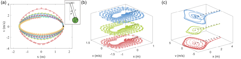
A.1 Oscillating pendulum
| (7) |
The training dataset contains 5 system instances with m. A long trajectory of 10 s is generated for each instance with the initial position and velocity and 0 and time marching stepsize 10 ms. During training, a batch of 20 trajectories of 1 s are pulled out randomly in each epoch. So essentially the iMODE training is seeing 1 s trajectories with differential initial conditions.
The learnt iMODE model is tested on 8 unseen system instances with m. The task adaptation is similarly done as the training, i.e., seeing a batch of 20 randomly pulled-out trajectories of 1 s for each testing system instance. The task adaptation only takes 5 steps. Then the learnt model for each instance is used to calculate a trajectory of 5 s given an initial condition, and compared with ground truth. The results are shown in Fig. S1(a). The solid lines (the ground truth) match well with the circles (prediction).
A.2 Bistable oscillator
| (8) |
The training dataset contains 20 system instances, a mesh of and . Trajectories of multiple initial conditions with stepsize 10 ms and time span 10 s are generated for each instance. During training, a batch of 100 randomly pulled-out trajectories of 1 s is used for each epoch. During testing, task adaptation takes 5 steps on previously unseen systems . The learnt models calculate trajectories of 5 s given an initial condition. The results are shown in Fig. S1(b).

A.3 Van der Pol system
| (9) |
The training dataset contains 27 system instances, a mesh of , , and . Trajectories of multiple initial conditions with stepsize 10 ms and time span 10 s are generated for each instance. During training, a batch of 100 randomly pulled-out trajectories of 1 s is used for each epoch. During testing, task adaptation takes 5 steps on previously unseen systems instances . The learnt models calculate trajectories of 5 s given an initial condition. The results are shown in Fig. S1(c).
The three variation directions in the latent space for , , and are shown in Fig. S2.
Appendix B Other systems

B.1 Wall bouncing system
The governing equation for the wall bouncing system (Fig. S3(a)) is
and are the particle position and velocity, N/m is a large constant to approximate a stiff wall, is the (half-)width of the potential well, as shown in Fig. S3(a). The system has a potential energy well with the following form
| (13) |
The training dataset contains 10 system instances, with the width increasing from 0.1 m to 1.0 m by 0.1 m. Trajectories of multiple initial conditions (initial position 0 m, and initial velocities ranging from 0.1 m/s to 1.0 m/s) with stepsize 10 ms and time span 10 s are generated for each instance. During training, a batch of 100 randomly pulled-out trajectories of 1 s is used for each epoch.
In this case the intermediate output of the NN is the energy and the force is derived by taking the derivative of the output with respect to the input, i.e.
| (14) |
The second equality takes advantage of the assumption that the energy is symmetric with respect to . The learning results show to be in perfect correlation with the width of the potential well (Fig. S4). In other words, we can control the width of the constructed potential well of the NN, which is another way to interpret the physical meaning of the adaptation parameter .
B.2 Double pendulum
The double pendulum, as shown in Fig. S3(b), has two masses kg and arm lengths and . The governing equations are
| (15) |
The training dataset contains 16 system instances, a mesh of m and m. Trajectories of initial locations [,] and initial velocities [0,0] with stepsize 10 ms and time span 10 s are generated for each system. During training, a batch of 100 randomly pulled-out trajectories of 1 s is used for each epoch. Task adaptation takes 5 steps. The learnt latent space of adaptation parameters is shown in Fig. S5. It is clear that two directions exist corresponding to the variation of physical parameters and . This again underlines the interpretability of .
Appendix C Comparison between iMODE and training from scratch
We compare the performance of iMODE adaptation to the “training from scratch” (TFS) approach. The iMODE adaptation starts with a weight initialization trained from a training dataset. It updates the adaptation parameter on a testing dataset, which is not included in the training dataset. The TFS approach uses the same NN architecture and hyperparameters as in the iMODE. The TFS NN is randomly initialized and all the weights are updated on the same testing dataset. After training the TFS NN and adapting the iMODE NN using the same testing dataset, the two NNs are evaluated on an unseen evaluation dataset. As shown in Fig. 3(a), the iMODE significantly outperforms the TFS approach in terms of adaptation speed (v.s. training speed in the TFS approach) and evaluation accuracy. This means that the iMODE approach can learn the dynamics of an unseen system more rapidly and predict future events more accurately than a TFS NN. This observation is pronounced in the following case: we feed these two NNs a single trajectory of the bistable system with physical parameters and , and initial condition m and m/s. After training/adaptation, we evaluate the TFS and iMODE NNs on trajectories of the same system but with differential initial conditions. The training/adaptation and evaluation curves are shown in Fig. S6(a). The iMODE outperforms the TFS approach in both training/adaptation and evaluation accuracy. The learnt energy functions of both approaches are compared in Fig. S6(b). The energy function of the TFS NN is totally incorrect due to the data scarcity. Under this specific initial condition, the bistable system is only oscillating intra-well. So the information contained in the trajectory is insufficient to depict the entire potential energy surface. Meanwhile the iMODE NN learns an accurate double-potential-well function from the same data because appropriate prior knowledge on the energy functions of bistable systems (i.e. double-well) is already embedded in its weight initialization.
Appendix D Dimension determination of physical parameters with PCA
The workflow of using PCA to determine the optimal dimension of the adaptation parameters for a parametric system is: (1) Make a rough guess on the dimension, then run the iMODE algorithm on the trajectories of systems; (2) Form a matrix with the results ; (3) Perform PCA on . A significant portion of variance (e.g. 99%) will be preserved in the first dimensions, an estimation for ; (4) repeat the process with different initial guesses . The optimal dimension is more credible when different results in the same .
The PCA determination results of all systems are shown in Fig. S7. The red dashed lines mark the variance preservation. Dotted lines in each case mean that the initial guess is the dimension of real physical parameters plus 2. For example, in the Van der Pol system, the dotted line means that the initial guess . After the PCA, if we preserve 4 or 3 principal components, the variance energy is still preserved by more than 99%. If we further reduce the number of preserved principal components to 2 or 1, we see a sudden drop (to below the 99% threshold), which indicates the optimal dimension to be 3. The for dashed-dotted and solid lines are the dimension of real physical parameters plus 1 and 0 respectively. With different , we can repeatedly confirm the optimal dimension of , to be 3 in the case of Van der Pol system (which is the true dimension of physical parameters). For other systems, the workflow is the same.
Appendix E Neural Gauge diffeomorphism
As suggested by the PCA analysis in Section SD, the adaptation parameters that are adapted to the system instances belonging to a family of dynamical systems occupy a -dimensional manifold, even if the latent space they reside in is -dimensional and . Therefore, a diffeomorphism can be established mapping in the latent space to their corresponding physical parameters () even if their dimensions do not match, assuming . Practically, the neural ODE modelling such diffeomorphism can be defined as , such that for , starting from a given point in the latent space, , the state at , is the concatenation of corresponding physical parameters and padding zeros.
Appendix F Complex cases
F.1 Slinky: the Euclidean symmetric neural network
The NN used in the Slinky case follows the Euclidean symmetric neural network (ESNN) Li2022Rapidly architecture. The Slinky is decomposed into 40 consecutive triplets, i.e., the 2D representation of 3 adjacent cycles. We denote the coordinates of the th triplet as . is the coordinates of the th bar, including the and coordinates of the bar center and the inclination angle of the bar. The potential energy associated with the middle bar of a triplet is only a function of the coordinates of the 3 bars of the same triplet (and of the adaptation parameters), i.e.
| (16) |
In the following we will omit the subscript for brevity. The induced force from is
| (17) |
where is the relative coordinates between the bars of the th triplet. We enforce Euclidean invariance, i.e., translational, rotational, and chiral invariance, on with respect to , by taking the following form, i.e., the ESNN
| (18) |
where and denote reflection with respect to the and axes. Note that
| (19) |
where is the identity operation. It is easy to prove the chiral invariance of , i.e.,
| (20) |
Then from Eq. (17), is equivariant to rigid body and chiral transformations on , as shown in Fig. S8, including translation, rotation, and reflection, regardless of . The ESNN will be applied on each triplet in the Slinky to calculate the elastic force acting on each bar. The assembled force vector is used to update the system state inside the NODE framework. The difference between the true and predicted trajectories is used to update the ESNN weights . After training and performing trajectory predictions in 2D, a geometric method can be used to reconstruct the 3D Slinky configurations Li2022Rapidly. See Li2022Rapidly for more implementation details.

The training dataset contains 4 Slinkies of different Young’s modulus (50, 60, 70, and 80 GPa). The Slinkies are clamped at both ends and freely drop under gravity from a horizontal initial configuration. Two inner steps are taken to update for each Slinky. Note when is updated, the NN always preserves energy invariance and force equivariance with respect to the coordinates of the Slinky. After training the NN, we perform task adaptation (2 steps) on a unseen Slinky of Young’s modulus 56 GPa and observe a good fitting result (Fig. S9(a)). The resulting NN is then directly applied to computation under an unseen boundary condition and Slinky orientation (the bottom end is free and the Slinky drops under gravity from a vertical initial configuration) without any modification (Fig. S9(b)). We can achieve this because the model-agnostic nature of the iMODE method allows us to embed the Euclidean symmetries into the NN.

F.2 Kolmogorov-Petrovsky-Piskunov (KPP) equation
To solve the KPP equation, we discretize the spatial domain [0,1] into 20 segments. So the the partial differential equation system (here denotes the spatial coordinate)
| (21) |
is represented by an ordinary differential equation system containing 21 variables. The diffusion term is approximated by 2nd-order central difference and the diffusivity is assumed known. The meta-learning is performed to learn the reaction term with different reaction strength coefficients (without knowing the mathematical form). The training dataset contains 5 systems with . The Neumann boundary condition ( denotes derivative with respect to ) is used across the training dataset. The iMODE task adaptation takes 5 iterations. The training results for are shown in Fig. S10(a). The iMODE NN is then adapted on the data from a unseen system instance with . The resulted NN is directly applied to computation with unseen initial and boundary conditions (Dirichlet type ). The results of the latter are shown in Fig. S10(b) and a good agreement is observed. This again validates the capability of the iMODE algorithm to fast adapt on unseen complex parametric systems and accurately predict on initial and boundary conditions different from those in the training dataset.
Another testing result for the KPP system is shown in Fig. S10(c). The testing has the same type of boundary condition () as the training dataset but an unseen initial condition. The prediction (right) matches the ground truth (left) well.
Appendix G Neural network architecture
Throughout this letter, we use a DenseNet-like architecture Huang2017Densely for our neural networks (NNs), where shortcut pathways are created for a layer from all its previous layers. It takes in the input and first increases the feature dimension to 32 by a fully-connected (FC) layer. Then the feature is passed through FC layers with Softplus activation. A new feature with an increased dimension is formed by concatenating the previous feature with the FC layer output, i.e.,
| (22) |
where is the feature map for the th layer. After passing through 5 densely connected layers, the feature dimension is increased to 192. This feature is then passed through a FC layer with no activation to produce the final output.
For pendulum, bistable, wall bouncing, and Slinky systems, the NN input is the vector concatenating the system position and the adaptation parameter , i.e. . The output is a scalar, i.e. the energy of the system. The force vector is calculated by back-propagating the NN output with respect to . For Van der Pol system, the input is the vector concatenating the system state and , i.e. . The output is the force vector. For KPP system, the input is . The output is the reaction forcing term.
Appendix H Supplementary movie
Movie S1. The diffeomorphism for the bistable system. The data points are transformed from the physical space (subtracted mean) to the latent space of adaptation parameters (subtracted mean). The right subplot is the enlarged view of the left plot.
Movie S2. The diffeomorphism for the Van der Pol system. The data points are transformed from the physical space (subtracted mean) to the latent space of adaptation parameters (subtracted mean). The right subplot is the enlarged view of the left plot.
References
- (1) Q. Li, T. Wang, V. Roychowdhury, M. Jawed, Rapidly encoding generalizable dynamics in a Euclidean symmetric neural network, Extreme Mechanics Letters (2022) 101925.
- (2) G. Huang, Z. Liu, L. Van Der Maaten, K. Q. Weinberger, Densely connected convolutional networks, in: 2017 IEEE Conference on Computer Vision and Pattern Recognition (CVPR), 2017, pp. 2261–2269.