Dijet azimuthal decorrelation in ${\boldsymbol{e^{+}e^{-}}}$ annihilationJournal: Physics Letters B

The origin of NGLs at two loops is the emission of a soft gluon $k_{1}$ inside any of the two outgoing jets which itself emits a softer gluon $k_{2}$ outside the jets without being clustered back to them. While this configuration results in a non-zero $\delta\phi$, its virtual correction (specifically when $k_{2}$ is virtual) gives $\delta\phi=0$, and thus we have a real-virtual mis-cancellation of the soft singularities. We express the contribution of the uncanceled virtual correction to the integrated azimuthal decorrelation distribution as follows

where $\mathrm{C_{A}}$ is the color factor associated with the non-Abelian emission of gluon $k_{2}$ off $k_{1}$. The irreducible two-loops antenna function $\mathcal{A}_{q\bar{q}}^{12}$ is given by [28]

with $s_{i}\equiv\sin\theta_{i}$. The function $\Xi^{\mathrm{NG}}_{2}$ restricts the angular phase-space of integration and is given, in the anti-$k_{t}$ and $k_{t}$ algorithms respectively, by

The step function $\Theta(d_{12}-d_{2})$ forbids gluon $k_{2}$ from being clustered back to the jet in the $k_{t}$ algorithm. It is given by $\Theta(\cos R-\cos\theta_{12})$, with $\cos\theta_{12}=c_{1}c_{2}+s_{1}s_{2}\cos(\phi_{1}-\phi_{2})$.

In the anti-$k_{t}$ algorithm the integration is simple and its result can be expressed in the same form as that of the rapidity-gap NGLs coefficient found in ref. [20]

where $\Delta\eta(R)$ is defined in eq. (9). The above formula shows that in the limit $R\to 0$ the two-loops NGLs coefficient does not vanish, but rather reaches its maximum value. This feature was observed in ref. [20] and was ascribed to the fact that NGLs originate from the edge of jets, since this is the phase-space region where gluons $k_{1}$ and $k_{2}$ are collinear and thus the amplitude squared (14) is most singular.

In the $k_{t}$ algorithm, and at small values of $R$ (using small angles), we can write the NGLs coefficient as

where we made the following changes of variables: $\phi=\phi_{1}-\phi_{2}$ and $\theta_{i}\to R\,\theta_{i}$. Away from the small-$R$ limit one may perform the integration numerically to obtain the full-$R$ result for the two-loops coefficient of NGLs. We present the results in the following subsection together with the CLs coefficient.

To compute the CLs we consider the Abelian primary emission of two strongly-ordered gluons directly off the hard $q\bar{q}$ dipole, whereby the harder gluon $k_{1}$ is inside one of the two jets and the softer $k_{2}$ is outside both of them, with the constraint $d_{12}<d_{2}$, such that gluon $k_{2}$ gets clustered into the jet by gluon $k_{1}$, which leads to $\delta\phi=0$. However, when $k_{1}$ is virtual then gluon $k_{2}$ remains in the gap causing the hard jets to decorrelate. In this case we obtain a large single logarithmic contribution to the $\delta\phi$ distribution given by

Note again that $\mathcal{C}^{\mathrm{ak}_{t}}_{2}(R)=0$, as there are no CLs for anti-$k_{t}$ clustering.

First, let us consider the small-$R$ limit of this integral. In this case we may write

Away from this small-$R$ limit we perform the integration numerically. We show in figure 2 a plot of the coefficients of NGLs and CLs at $\mathcal{O}(\alpha_{s}^{2})$ as a function of the jet radius $R$. Also shown is the combined coefficient of CLs and NGLs in the $k_{t}$ algorithm; $\mathcal{F}^{\mathrm{k}_{t}}_{2}=\mathcal{S}^{\mathrm{k}_{t}}_{2}+\mathcal{C}^{\mathrm{k}_{t}}_{2}$.

Notice that the NGLs coefficient in $k_{t}$ clustering is significantly smaller than that in anti-$k_{t}$. Physically, this can be explained by the fact that the $k_{t}$ clustering procedure reduces the angular phase space available for collinear enhancement of the two gluons near the boundaries of the jets. This reduction of NGLs was reported even at NLL accuracy [27]. The CLs coefficient is positive and quite small, with the advantage that it cancels the NGLs coefficient, particularly at small values of $R$. Note that the overall coefficient $\mathcal{F}_{2}$ is less than 1 for values of $R$ smaller than about $0.5$. For small $R$ values, the anti-$k_{t}$ NGLs coefficient computed here is identical to that found for the single hemisphere mass [29] and jet mass with a jet veto [27].

We compare our two-loops results with the exact MC distribution at $\mathcal{O}(\alpha_{s}^{2})$ obtained with the EVENT2 program. The latter splits the distribution at NLO into three color contributions; $\mathcal{O}(\mathrm{C_{F}^{2}})$, $\mathcal{O}(\mathrm{C_{F}}\,\mathrm{C_{A}})$ and $\mathcal{O}(\mathrm{C_{F}}\,\mathrm{T_{f}}\,\mathrm{n_{f}})$, with $\mathrm{T_{f}}=1/2$ being the normalization constant of the generators of the SU(3) group in the fundamental representation and $\mathrm{n_{f}}=5$ is the number of active quark flavors. The expansion of the resummed distribution at this order, including running coupling effects, is written, after differentiating with respect to $L$, as

At this order this differential distribution is linear in $L$, but does not capture the $\mathcal{O}(1)$ constant, which, in the cumulative integrated distribution, is an NLL $\mathcal{O}(\alpha_{s}^{2}\,L)$ term. We plot the difference between the MC distribution and the expansion (20) for each color contribution separately. All curves should tend towards a constant when $L$ grows large and negative. The results are shown in figure 3. Here the $\mathcal{O}(\mathrm{C_{F}^{2}})$ part contains the CLs coefficient in $k_{t}$ clustering, while the $\mathcal{O}(\mathrm{C_{F}}\,\mathrm{C_{A}})$ term contains the NGLs coefficient both in $k_{t}$ and anti-$k_{t}$ algorithms. The $\mathcal{O}(\mathrm{C_{F}\,T_{f}\,n_{f}})$ contribution is algorithm independent at LL accuracy, but the NLL $\mathcal{O}(1)$ constant does depend on the jet algorithm.

At $\mathcal{O}(\alpha_{s}^{3})$, the cumulative distribution can be written as follows

Focusing first on the pure NGLs contribution $\Sigma_{3}^{\mathrm{NG}}$ (i.e., excluding the cross-talk between the one-loop global and two-loops non-global logarithms) in the anti-$k_{t}$ algorithm, we may write it in the form

where we define $\bar{\mathcal{A}}_{q\bar{q}}^{13}=\mathcal{A}_{q\bar{q}}^{13}/\omega_{q\bar{q}}^{1}$, and the 3-loops irreducible cascade antenna function is given by

It is worth mentioning that, for the cascade term, there is a non-negligible contribution from the configuration in which gluon $k_{1}$ is in one jet emitting gluon $k_{2}$ in the other jet which itself emits the softest gluon $k_{3}$ in the gap between the two jets. At small values of $R$ the integration is quite simple and yields the result

Notice that this result is twice that found for the hemisphere mass observable [30]. Away from the small-$R$ limit the integration can be performed numerically and we shall present the results in the next subsection.

The pure NGLs contribution in the $k_{t}$ algorithm is given by an identical form to that of the anti-$k_{t}$ (22a)

We perform for the first time in the literature a calculation of NGLs in the $k_{t}$ algorithm beyond two loops. Due to non-linearity of $k_{t}$ clustering we shall find a class of NGLs that have a non-standard color factor, namely $\mathrm{C_{F}^{2}}\,\mathrm{C_{A}}$ at $\mathcal{O}(\alpha_{s}^{3})$. Such terms usually (in anti-$k_{t}$ clustering) only arise in the cross-talk of the expansion of the primary-emission global form factor (10) at $\mathcal{O}(\alpha_{s})$ together with NGLs at $\mathcal{O}(\alpha_{s}^{2})$, i.e., the term $\Sigma_{1}(\Delta)\times\Sigma_{2}^{\mathrm{NG}}(\Delta)$ in eq. (21). However, in the $k_{t}$ algorithm, we find them as “pure” irreducible NGLs. That is, they are part of the term $\Sigma_{3}^{\mathrm{NG}}(\Delta)$ in eq. (21).

To proceed, we consider three types of emissions at $\mathcal{O}(\alpha_{s}^{3})$, as shown in figure 4: (a) one primary + two correlated emissions, (b) ladder emissions, and (c) cascade emissions. In each case we consider all possible virtual-correction Feynman diagrams as well as angular configurations of the emitted gluons that affect the clustering procedure, and look for a mis-match between the soft divergences of these emissions.

Starting first with type (a) contributions, there are three possible permutations of the gluons. ²² 2 Note that for all permutations the transverse momenta of the three gluons are strongly ordered as follows: $k_{t1}\gg k_{t2}\gg k_{t3}$. For the permutation in which $k_{3}$ is emitted in correlation with $k_{2}$, and which has a squared amplitude $4\,\mathrm{C_{F}^{2}}\,\mathrm{C_{A}}\,\omega_{q\bar{q}}^{1}\,\mathcal{A}_{q\bar{q}}^{23}$, we find that the angular phase space of integration that yields a logarithmic contribution is given by

To see how one obtains this result let us give one example of angular configurations that result in a logarithmic contribution. There are four Feynman diagrams in this case, shown in figure 5. Consider the situation when particles $k_{3}$ and $k_{2}$ are outside the jet regions, $d_{3j}>d_{3}$ and $d_{2j}>d_{2}$, while particle $k_{1}$ is inside, $d_{1j}<d_{1}$. In this scenario, both diagrams in which $k_{1}$ is virtual (i.e., diagrams (3) and (4) in figure 5) yield $\delta\phi\neq 0$, since in both diagrams particle $k_{2}$ is real and remains in the gap region after applying the clustering. However, these two diagrams contribute equally and with opposite signs, so they cancel each other. For the remaining two diagrams, (1) and (2), we have a mismatch when particle $k_{2}$ gets pulled inside the jet by the real particle $k_{1}$ while $k_{3}$ remains in the gap. This happens when $d_{12}$ is smaller than $d_{2}$, and both $d_{13}$ and $d_{23}$ are greater than $d_{3}$. While in diagram (1) we have a real unclustered gluon $k_{3}$ in the gap region (i.e., it forms a jet on its own) giving $\delta\phi\neq 0$, in diagram (2) the gap is empty and the hard jets are exactly back-to-back with $\delta\phi=0$. The virtual-correction diagram (2) contributes fully to the cumulative distribution while the real-emission diagram (1) cancels this contribution only up to $\delta\phi=\Delta$, leaving uncanceled virtual-correction contributions with a negative sign. This is the last term in eq. (26).

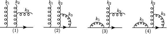
Similarly, we obtain for the second and third gluon permutations of type (a) diagrams, with squared amplitudes $4\,\mathrm{C_{F}^{2}}\,\mathrm{C_{A}}\,\omega_{q\bar{q}}^{2}\,\mathcal{A}_{q\bar{q}}^{13}$ and $4\,\mathrm{C_{F}^{2}}\,\mathrm{C_{A}}\,\omega_{q\bar{q}}^{3}\,\mathcal{A}_{q\bar{q}}^{12}$, respectively, as well as type (b) (ladder-emission) contributions, with squared amplitude $2\,\mathrm{C_{F}}\,\mathrm{C_{A}^{2}}\,\bar{\mathcal{A}}_{q\bar{q}}^{12}\,\mathcal{A}_{q\bar{q}}^{13}$, the same phase space function. It is given by

Finally, for type (c) (cascade emission) contributions, corresponding to the squared amplitude $2\,\mathrm{C_{F}}\,\mathrm{C_{A}^{2}}\,\mathcal{B}_{q\bar{q}}^{123}$, the phase space function reads

Before performing the integration, we subtract off the part of the phase space that produces the interference term between the one-loop global primary logarithm and the two-loops NGLs, which only comes from type (a) emissions. For the first permutation of gluons, this part of phase space is identified by the second term in eq. (26), $\Theta_{\mathrm{out}}(k_{1})\Theta_{\mathrm{in}}(k_{2})\Theta_{\mathrm{out}}(k_{3})\Theta(d_{23}-d_{3})$, where gluon $k_{1}$ reproduces the one-loop global term (8) and the other correlated gluons, $k_{2}$ and $k_{3}$, give the two-loops NGLs (eq. (13b) with phase space (15b)). However, for the other two gluon permutations of type (a) emissions, the phase space (27) does not simply contain such interference terms. Strictly speaking, this means that NGLs do not cleanly factorize from the global form factor in the $k_{t}$ algorithm. Nevertheless, we can manually add and subtract the interference terms and write the total distribution in the factorizable form (21).

We can then write the “pure” NGLs coefficient $\mathcal{S}_{3}^{\mathrm{k}_{t}}$, given in eq. (25), in the following form

where we split the result according to the color factor, such that for type (a) emissions we have

with modified phase space that subtracts away the interference terms

and for type (b) and (c) emissions

We are now in a position to perform the integrations numerically as a function of the jet radius $R$. We show the results in the next subsection, in which we also compute the clustering logarithmic contribution at $\mathcal{O}(\alpha_{s}^{3})$.

Following the same steps as for NGLs calculation, the phase space clustering function at $\mathcal{O}(\alpha_{s}^{3})$ for the CLs contribution, which results from the mismatch of soft singularities between real and virtual emissions of three primary soft gluons, with a squared amplitude $8\,\mathrm{C_{F}^{3}}\,w_{q\bar{q}}^{1}\,w_{q\bar{q}}^{2}\,w_{q\bar{q}}^{3}$, is given by

Note that the above phase-space clustering function is similar (but not exactly identical) to that found for the jet mass observable [31]. Extracting the interference terms between the CLs at two loops and the global logarithm at one loop, i.e., the term $\Sigma_{1}(\Delta)\times\Sigma_{2}^{\mathrm{CL}}(\Delta)$ in eq. (21), we reduce the above phase space function to that of the “pure” CLs contribution as

Then, the clustering logarithmic contribution to the cumulative cross-section is given by

We show in figure 6 a plot of the coefficients of NGLs and CLs in the $k_{t}$ and anti-$k_{t}$ algorithms as a function of the jet radius $R$. Shown also is the combined coefficient $\mathcal{F}^{\mathrm{k}_{t}}_{3}=\mathcal{S}_{3}^{\mathrm{k}_{t}}+\mathcal{C}_{3}^{\mathrm{k}_{t}}$ for the $k_{t}$ algorithm.

As in the previous section, we notice that the NGLs coefficient in the anti-$k_{t}$ algorithm at this order is also quite large. Clearly, the application of the $k_{t}$ clustering has reduced the significance of NGLs by almost a factor of 30 for values less than $R\sim 0.6$. The CLs coefficient is also small such that the overall coefficient $\mathcal{F}_{3}$ is smaller in magnitude than the $\mathcal{S}_{3}^{\mathrm{ak}_{t}}$ by about a factor of 3 for most values of $R$.

The calculation of NGLs with anti-$k_{t}$ clustering proceeds in a similar manner at fourth order, and can easily be deduced from previous calculations of NGLs in the literature. In fact, the phase space of integration is similar to that of the hemisphere mass distribution reported in ref. [30], and thus the cumulative cross-section, at this order, may be cast in the following way

with pure NGLs contribution given by

References

- Hautmann and Jung [2008] F. Hautmann, H. Jung, JHEP 10 (2008) 113. arXiv:0805.1049.
- Aktas et al. [2004] A. Aktas, et al. (H1), Eur. Phys. J. C 33 (2004) 477–493. arXiv:hep-ex/0310019.
- Aaboud et al. [2018] M. Aaboud, et al. (ATLAS), Phys. Rev. D 98 (2018) 092004. arXiv:1805.04691.
- Aad et al. [2011] G. Aad, et al. (ATLAS), Phys. Rev. Lett. 106 (2011) 172002. arXiv:1102.2696.
- Sirunyan et al. [2018] A. M. Sirunyan, et al. (CMS), Eur. Phys. J. C 78 (2018) 566. arXiv:1712.05471.
- Abazov et al. [2005] V. Abazov, et al. (D0), Phys. Rev. Lett. 94 (2005) 221801. arXiv:hep-ex/0409040.
- Aaboud et al. [2019] M. Aaboud, et al. (ATLAS), Phys. Rev. C 100 (2019) 034903. arXiv:1901.10440.
- Banfi et al. [2008] A. Banfi, M. Dasgupta, Y. Delenda, Phys. Lett. B 665 (2008) 86–91. arXiv:0804.3786.
- Chatrchyan et al. [2013] S. Chatrchyan, et al. (CMS), Phys. Lett. B 722 (2013) 238–261. arXiv:1301.1646.
- Andreev et al. [2022] V. Andreev, et al. (H1), Phys. Rev. Lett. 128 (2022) 132002. arXiv:2108.12376.
- Liu et al. [2020] X. Liu, F. Ringer, W. Vogelsang, F. Yuan, Phys. Rev. D 102 (2020) 094022. arXiv:2007.12866.
- Abramowicz et al. [2018] H. Abramowicz, et al. (ZEUS), JHEP 01 (2018) 032. arXiv:1712.04273.
- Catani et al. [1993] S. Catani, Y. L. Dokshitzer, M. H. Seymour, B. R. Webber, Nucl. Phys. B 406 (1993) 187–224.
- Ellis and Soper [1993] S. D. Ellis, D. E. Soper, Phys. Rev. D 48 (1993) 3160–3166. arXiv:hep-ph/9305266.
- Cacciari et al. [2012] M. Cacciari, G. P. Salam, G. Soyez, Eur. Phys. J. C 72 (2012) 1896. arXiv:1111.6097.
- Cacciari et al. [2008] M. Cacciari, G. P. Salam, G. Soyez, JHEP 04 (2008) 063. arXiv:0802.1189.
- Dokshitzer et al. [1997] Y. L. Dokshitzer, G. D. Leder, S. Moretti, B. R. Webber, JHEP 08 (1997) 001. arXiv:hep-ph/9707323.
- Wobisch and Wengler [1998] M. Wobisch, T. Wengler, in: Workshop on Monte Carlo Generators for HERA Physics (Plenary Starting Meeting), pp. 270–279. arXiv:hep-ph/9907280.
- Dasgupta and Salam [2001] M. Dasgupta, G. Salam, Phys. Lett. B 512 (2001) 323–330. arXiv:hep-ph/0104277.
- Dasgupta and Salam [2002] M. Dasgupta, G. P. Salam, JHEP 03 (2002) 017. arXiv:hep-ph/0203009.
- Banfi and Dasgupta [2005] A. Banfi, M. Dasgupta, Phys. Lett. B 628 (2005) 49–56. arXiv:hep-ph/0508159.
- Delenda et al. [2006] Y. Delenda, R. Appleby, M. Dasgupta, A. Banfi, JHEP 12 (2006) 044. arXiv:hep-ph/0610242.
- Catani and Seymour [1997] S. Catani, M. H. Seymour, Nucl. Phys. B 485 (1997) 291–419. arXiv:hep-ph/9605323, [Erratum: Nucl.Phys.B 510, 503–504 (1998)].
- Catani and Seymour [1996] S. Catani, M. H. Seymour, Phys. Lett. B 378 (1996) 287–301. arXiv:hep-ph/9602277.
- Banfi et al. [2021] A. Banfi, F. A. Dreyer, P. F. Monni, JHEP 10 (2021) 006. arXiv:2104.06416.
- Banfi et al. [2022] A. Banfi, F. A. Dreyer, P. F. Monni, JHEP 03 (2022) 135. arXiv:2111.02413.
- Khelifa-Kerfa [2012] K. Khelifa-Kerfa, JHEP 02 (2012) 072. arXiv:1111.2016.
- Delenda and Khelifa-Kerfa [2016] Y. Delenda, K. Khelifa-Kerfa, Phys. Rev. D 93 (2016) 054027. arXiv:1512.05401.
- Banfi et al. [2010] A. Banfi, M. Dasgupta, K. Khelifa-Kerfa, S. Marzani, JHEP 08 (2010) 064. arXiv:1004.3483.
- Khelifa-Kerfa and Delenda [2015] K. Khelifa-Kerfa, Y. Delenda, JHEP 03 (2015) 094. arXiv:1501.00475.
- Delenda and Khelifa-Kerfa [2012] Y. Delenda, K. Khelifa-Kerfa, JHEP 09 (2012) 109. arXiv:1207.4528.
- Hatta and Ueda [2013] Y. Hatta, T. Ueda, Nucl. Phys. B 874 (2013) 808–820. arXiv:1304.6930.
- Hagiwara et al. [2016] Y. Hagiwara, Y. Hatta, T. Ueda, Phys. Lett. B 756 (2016) 254–258. arXiv:1507.07641.
- Hatta and Ueda [2021] Y. Hatta, T. Ueda, Nucl. Phys. B 962 (2021) 115273. arXiv:2011.04154.