Reduced quiver quantum toroidal algebras

Andrei Negu t , Address: MIT, Department of Mathematics, Cambridge, MA, USA Address: Simion Stoilow Institute of Mathematics, Bucharest, Romania Email address: andrei.negut@gmail.com

Abstract.

We give a generators-and-relations description of the reduced versions of quiver quantum toroidal algebras, which act on the spaces of BPS states associated to (non-compact) toric Calabi-Yau threefolds $X$ . As an application, we obtain a description of the $K$ -theoretic Hall algebra of (the quiver with potential associated to) $X$ , modulo torsion.

1. Introduction

1.1.

Let $X$ be a (non-compact) toric Calabi-Yau threefold. To $X$ one can associate a 2d quantum field theory with four supercharges, and we will be interested in two features of this theory: its vector space of BPS states, and more importantly for us, the BPS algebra which acts on said vector space. The latter algebra has been dubbed the quiver quantum toroidal algebra ([4, 5, 13, 14], following [9]).

Before we dive into the definition of the quiver quantum toroidal algebra ${\widetilde{\mathbf{U}}}$ , let us recall certain objects associated to the Calabi-Yau threefold $X$

X\leadsto\text{toric diagram}\leadsto\text{brane tiling}\leadsto\text{quiver}

We refer the reader to [14, Appendix C] for a detailed review of the procedures $\leadsto$ listed above, and we simply contend ourselves with stating the following properties of the objects involved.

•

The toric diagram associated to $X$ is a particular collection of points in ${\mathbb{Z}}^{2}$ and line segments between them.
•

The normals to the aforementioned line segments can be drawn on the torus ${\mathbb{T}}^{2}$ , and they define a brane tiling, i.e. a decomposition of the torus into polygonal regions called faces. Very importantly, the faces can be colored in blue and red such that any two faces which share an edge have different colors. ¹¹ 1 As just described, the brane tiling is a graph $G$ drawn on the torus. In the literature, the term “brane tiling” is sometimes applied to the dual graph of $G$ , which is bipartite.
•

The vertices and edges of the aforementioned faces determine a quiver $Q$ drawn on ${\mathbb{T}}^{2}$ . The bicolorability property of the brane tiling implies that the edges of $Q$ can be oriented so that they go clockwise around the blue faces and counterclockwise around the red faces. The interested reader may find the quiver associated to the Calabi-Yau threefold $X={\mathbb{C}}^{3}$ in Figure 1.

Refer to caption — Figure 1. The quiver associated to $X={\mathbb{C}}^{3}$ . The above square is the usual representation of the flat torus, so the quiver has one vertex, three edges and two faces.

1.2.

As the definition of the quiver quantum toroidal algebra ${\widetilde{\mathbf{U}}^{+}}$ only takes the quiver as input, one can state the construction in generality greater than those quivers which arise from toric Calabi-Yau threefolds via the procedure above.

Definition 1.3.

Let $Q$ be a quiver drawn on a torus (with vertex set $I$ and edge set $E$ ), whose faces are colored in blue and red such that the two incident faces to a given edge have different colors. We assume that the edges of the quiver are oriented so as to go clockwise around the blue faces.

We will write $\widetilde{Q}$ for the lift of $Q$ to the universal cover ${\mathbb{R}}^{2}$ of ${\mathbb{T}}^{2}$ , and note that $\widetilde{Q}$ inherits the blue/red colored faces of $Q$ . In the present paper, “paths” and “cycles” in a quiver will refer to the oriented notions.

Definition 1.4.

A broken wheel refers to a path obtained by removing a single edge $e$ from the boundary of any face $F$ of $\widetilde{Q}$ . The mirror image of the aforementioned broken wheel is the path obtained by removing $e$ from the boundary of the other face $F^{\prime}\neq F$ incident to $e$ . The edge $e$ will be called the interface of the broken wheel (and of its mirror image).

Definition 1.5.

The quiver $Q$ is called shrubby if given any paths $p\neq p^{\prime}$ in $\widetilde{Q}$ with the same start and end points, at least one of $p$ and $p^{\prime}$ contains a broken wheel whose interface lies in the closed region between the two paths.

When one of $p$ and $p^{\prime}$ is trivial, Definition 1.5 states that any cycle in $\widetilde{Q}$ must contain a broken wheel in the closure of its interior. We will see in Lemma 4.3 that the shrubbiness condition above is implied by more traditional notions of consistency of brane tilings and dimer models, such as the existence of a non-degenerate $R$ -charge. We do not know (and it is an interesting question) whether all quivers which arise from Calabi-Yau threefolds as in Subsection 1.1 are shrubby.

1.6.

Let ${\mathbb{K}}$ be a field of characteristic 0. To every edge $e$ of the quiver $Q$ , we associate a parameter $t_{e}\in{\mathbb{K}}^{\times}$ such that for every face $F$ of $Q$ we have ²² 2 In the setting of toric Calabi-Yau threefolds $X$ , one usually takes ${\mathbb{K}}={\mathbb{Q}}(q_{1},q_{2})$ where $q_{1},q_{2}$ are elementary characters of the rank 2 torus that acts on $X$ by preserving the Calabi-Yau 3-form. In this setting, the parameters $t_{e}$ are monomials in $q_{1}$ and $q_{2}$ .

(1.1)

\prod_{e\text{ edge around }F}t_{e}=1

We make the following genericity assumption on the parameters $\{t_{e}\}_{e\text{ edge}}$ .

Assumption 1.7.

There exists a field homomorphism $\rho:{\mathbb{K}}\rightarrow{\mathbb{C}}$ such that

(1.2)

\left|\prod_{e\text{ edge along }p}\rho(t_{e})\right|\neq\left|\prod_{e\text{ edge along }p^{\prime}}\rho(t_{e})\right|

for any paths $p$ and $p^{\prime}$ in $\widetilde{Q}$ with the same end point but different starting points.

In [9] and related works, products of the parameters $t_{e}$ along paths in $\widetilde{Q}$ are interpreted as coordinate functions of atoms in crystals; in this language, condition (1.2) is equivalent to requiring that different atoms have different coordinates. Thus, Assumption 1.7 holds in the physical settings that motivated the present paper.

The edge parameters can be assembled into the following rational functions

(1.3)

\zeta_{ij}(x)=\frac{\alpha_{ij}x^{s_{ij}}}{(1-x)^{\delta_{ij}}}\prod_{e\text{ arrow from }i\text{ to }j}(1-xt_{e})\in{\mathbb{K}}(x)

for all $i,j\in I$ , where $\alpha_{ij}\in{\mathbb{K}}^{\times}$ and $s_{ij}\in{\mathbb{Z}}$ are suitably chosen (but will not play an important role in the present paper, so we will not specify them explicitly).

Remark 1.8.

Moreover, different authors use different conventions on $\alpha_{ij}$ and $s_{ij}$ . For example, [4] requires $s_{ij}$ to be minus half the number of arrows from $i$ to $j$ ; this situation can also be accommodated by the present paper, at the cost of replacing polynomials built out of integer powers by polynomials built out of half-integer powers. We will avoid this setup in order to not overburden our notation.

1.9.

Using the data in Subsection 1.6, we will now review the definition of the quantum toroidal algebra associated to the quiver $Q$ and parameters $\{t_{e}\}_{e\in E}$ , which was introduced in [4, 13] as a trigonometric version of the quiver Yangian of [9] (see also [16] for a closely related mathematical construction).

Definition 1.10.

The (half) quiver quantum toroidal algebra ${\widetilde{\mathbf{U}}^{+}}$ is

(1.4)

{\widetilde{\mathbf{U}}^{+}}={\mathbb{K}}\Big\langle e_{i,d}\Big\rangle_{i\in I,d\in{\mathbb{Z}}}\Big/\text{relation \eqref{eqn:rel quad}}

where if we write

e_{i}(z)=\sum_{d\in{\mathbb{Z}}}\frac{e_{i,d}}{z^{d}}

then the defining relations are given by the formula

(1.5)

e_{i}(z)e_{j}(w)\zeta_{ji}\left(\frac{w}{z}\right)=e_{j}(w)e_{i}(z)\zeta_{ij}\left(\frac{z}{w}\right)

for all $i,j\in I$ . ³³ 3 Relation (1.5) is interpreted as an infinite collection of relations obtained by equating the coefficients of all $\{z^{a}w^{b}\}_{a,b\in{\mathbb{Z}}}$ in the left and right-hand sides (if $i=j$ , one clears the denominators $z-w$ from (1.5) before equating coefficients).

Define ${\widetilde{\mathbf{U}}^{-}}={\widetilde{\mathbf{U}}}^{+,\text{op}}$ , and denote its generators by $f_{i,d}$ instead of $e_{i,d}$ . Finally, let us consider the commutative algebra

\mathbf{U}^{0}={\mathbb{K}}\left[h_{i,d},h^{\prime}_{i,d^{\prime}}\right]_{i\in I,d,d^{\prime}\geq\text{appropriately chosen integers}}

Then the (full) quiver quantum toroidal algebra is defined as

(1.6)

{\widetilde{\mathbf{U}}}={\widetilde{\mathbf{U}}^{+}}\otimes\mathbf{U}^{0}\otimes{\widetilde{\mathbf{U}}^{-}}

with certain commutation relations imposed between elements in the three tensor factors above. We refer the reader to [4, 13] for the explicit commutation relations, as they will not be used in the present paper; instead, we will only focus on ${\widetilde{\mathbf{U}}^{+}}$ .

1.11.

The main motivation for defining the algebra ${\widetilde{\mathbf{U}}}$ is that it acts on the vector space of so-called BPS crystal configurations

(1.7)

{\widetilde{\mathbf{U}}}\curvearrowright M=\bigoplus_{\Lambda\text{ 3d crystal configuration}}{\mathbb{K}}\cdot|\Lambda\rangle

(see [13, Section 5] for a review of 3d crystal configurations, which are generalizations of plane partitions). We will not make the action (1.7) explicit, so we will not make any rigorous claims about it and merely use it as motivation for our subsequent constructions. The main goal of the present paper is to describe the kernel of the action (1.7), i.e. to define the smallest possible quotient

(1.8)

{\widetilde{\mathbf{U}}}\twoheadrightarrow\mathbf{U}

such that the action (1.7) factors through an action of $\mathbf{U}$ . To this end, we will consider the shuffle algebra realization of quiver quantum toroidal algebras

{\widetilde{\mathbf{U}}^{\pm}}\xrightarrow{\widetilde{\Upsilon}^{\pm}}{\mathcal{V}}^{\pm}=\bigoplus_{\bm{n}\in{\mathbb{N}}^{I}}{\mathbb{K}}[z_{i1},z_{i1}^{-1},\dots,z_{in_{i}},z_{in_{i}}^{-1}]_{i\in I}^{\textrm{sym}}

(we refer the reader to Subsection 2.1 for a description of the shuffle product on ${\mathcal{V}}^{\pm}$ , and to Subsection 2.3 for the definition of the homomorphism $\widetilde{\Upsilon}^{\pm}$ ). Set

(1.9)

\mathbf{U}^{\pm}={\widetilde{\mathbf{U}}^{\pm}}\Big/\text{Ker }\widetilde{\Upsilon}^{\pm}

As noted in [4, Section 5], the action (1.7) factors through the shuffle algebra. Therefore, the reduced (full) quiver quantum toroidal algebra

(1.10)

\mathbf{U}=\mathbf{U}^{+}\otimes\mathbf{U}^{0}\otimes\mathbf{U}^{-}

will inherit an action on $M$ from (1.7). To define this action, one needs to impose the same commutation relations between the tensor factors of (1.10) as between the tensor factors of (1.6). We will not present these relations explicitly in the present paper, and make no rigorous claims about them. Instead, we will focus on $\mathbf{U}^{+}$ .

1.12.

The main purpose of the present paper is to describe $\mathbf{U}^{\pm}$ by explicitly presenting the quotient (1.9). More specifically, we will describe a collection of generators for the two-sided ideal $\text{Ker }\widetilde{\Upsilon}^{\pm}$ . For every face $F=\{i_{0},i_{1},\dots,i_{k-1},i_{k}=i_{0}\}$ of the quiver $Q$ (note that some of the indices $i_{0},\dots,i_{k-1}$ may be repeated within a given face), consider the following parameters corresponding to the edges of $F$

(1.11)

t_{a}=t_{\overrightarrow{i_{a-1}i_{a}}}

Note that $t_{1}\dots t_{k}=1$ due to (1.1). Let $\widetilde{\zeta}_{ij}(x)=\zeta_{ij}(x)(1-x)^{\delta_{ij}}$ for all $i,j\in I$ . Then we may define the formal series

(1.12)

e_{F}(x_{1},\dots,x_{k})\in{\widetilde{\mathbf{U}}^{+}}[[x_{1},x_{1}^{-1},\dots,x_{k},x_{k}^{-1}]]

by the following formula

(1.13)

\sum_{a=1}^{k}\frac{x_{1}t_{2}\dots t_{a}}{x_{a}}\cdot\frac{\prod_{b\succ c}\widetilde{\zeta}_{i_{c}i_{b}}\left(\frac{x_{c}}{x_{b}}\right)\left(-\frac{x_{b}}{x_{c}}\right)^{\delta_{i_{b}i_{c}}\delta_{b<c}}}{\prod_{b\sim c+1}\left(1-\frac{x_{c}t_{b}}{x_{b}}\right)}\cdot\\ \cdot e_{i_{a}}(x_{a})\dots e_{i_{1}}(x_{1})e_{i_{k}}(x_{k})\dots e_{i_{a+1}}(x_{a+1})

In (1.13), the notation $b\succ c$ (respectively $b\sim c+1$ ) means that $b$ precedes (respectively immediately precedes) $c$ in the sequence $(a,\dots,1,k,\dots,a+1)$ . The symbols $\delta_{b<c}$ and $\delta_{i_{b}i_{c}}$ are defined as in Subsection 3.1. Note that the first line of (1.13) is a Laurent polynomial in $x_{1},\dots,x_{k}$ , due to the fact that all the denominators

1-\frac{x_{c}t_{b}}{x_{b}}

are canceled by the $\widetilde{\zeta}$ functions in the numerator. The following is our main result.

Theorem 1.13.

If $Q$ is shrubby (as in Definition 1.5), then the coefficients of the series (1.12) generate $\emph{Ker}\widetilde{\Upsilon}^{+}$ as a two-sided ideal. In other words, we have

(1.14)

\mathbf{U}^{+}={\widetilde{\mathbf{U}}^{+}}\Big/\Big(\text{series coefficients of }e_{F}(x_{1},\dots,x_{k})\Big)_{F\text{ face of }Q}

Similar results hold for $\mathbf{U}^{-}$ , by replacing $e$ ’s with $f$ ’s and reversing the order of the factors in the product on the second line of (1.13). ⁴⁴ 4 While the quotient (1.14) imposes a ${\mathbb{Z}}^{k}$ -worth of relations for every face $F$ with $k$ vertices, we will see in Remark 3.8 that these can be reduced to a ${\mathbb{Z}}$ -worth of relations for every face. More precisely, arbitrarily choosing one non-zero coefficient of the series $e_{F}$ in each integer homogeneous degree instead of all coefficients (for every face $F$ ) would determine the same quotient in (1.14).

Lemma 4.3 implies that a large family of physically interesting Calabi-Yau threefolds $X$ correspond to shrubby quivers, and so Theorem 1.13 applies to them. We conclude that the relations which we factor in (1.14) are the sought-for “Serre relations” of [4]. The terminology of these relations is historically motivated by the analogous situation of quantum loop groups associated to finite type Dynkin diagrams, in which the role of relations (1.14) is played by the Drinfeld-Serre relations. Note, however, that the classic Drinfeld-Serre relations are not enough to characterize quantum loop groups associated to general Dynkin diagrams (see [12]).

Remark 1.14.

If $Q$ is not shrubby, then we expect that one needs additional relations besides (1.13). In this situation, the ideal $\emph{Ker}\widetilde{\Upsilon}^{+}$ can be studied according to the general principles of [11], but we do not know explicit generators of this ideal.

Remark 1.15.

It is straightforward to write down rational/elliptic versions of the relations (1.13), which would give necessary relations that hold in the rational/elliptic counterparts of the reduced algebra $\mathbf{U}^{+}$ (see [4] for an overview). However, in the rational/elliptic settings, we do not know whether these relations are also sufficient, i.e. if they generate the analogue of the two-sided ideal $\emph{Ker}\widetilde{\Upsilon}^{+}$ .

1.16.

Let us spell out the constructions above in the case $X={\mathbb{C}}^{3}$ , when the quiver is the one in Figure 1. There is a single vertex, so $I=\{\bullet\}$ and we will henceforth suppress the indices $i\in I$ from all our formulas. There are three edges, whose associated parameters $t_{1},t_{2},t_{3}$ satisfy the equation

t_{3}=\frac{1}{t_{1}t_{2}}

We take the ground field to be ${\mathbb{K}}={\mathbb{Q}}(t_{1},t_{2})$ . The only $\zeta$ function (1.3) is

\zeta(x)=\frac{x^{-1}(1-xt_{1})(1-xt_{2})(1-xt_{3})}{1-x}

(the particular choice of the monomial $x^{-1}$ was made in order to match existing conventions in the literature). The (half) quiver quantum toroidal algebra (1.4) is generated by a single formal series $e(z)$ modulo the quadratic relation

(1.15)

e(z)e(w)(z-wt_{1})(z-wt_{2})(z-wt_{3})=\\ =e(w)e(z)(zt_{1}-w)(zt_{2}-w)(zt_{3}-w)

Meanwhile, formula (1.13) for the red face in Figure 1 reads

(1.16)

\begin{split}e_{F_{\text{red}}}(x_{1},x_{2},x_{3})=\frac{\prod_{i=1}^{3}[(x_{1}-x_{2}t_{i})(x_{1}-x_{3}t_{i})(x_{3}-x_{2}t_{i})]}{x_{1}x_{2}^{3}x_{3}^{3}(x_{1}-x_{3}t_{1})(x_{3}-x_{2}t_{3})}e(x_{1})e(x_{3})e(x_{2})\\ +\frac{t_{2}\prod_{i=1}^{3}[(x_{2}-x_{1}t_{i})(x_{1}-x_{3}t_{i})(x_{2}-x_{3}t_{i})]}{x_{2}^{3}x_{3}^{4}(x_{2}-x_{1}t_{2})(x_{1}-x_{3}t_{1})}e(x_{2})e(x_{1})e(x_{3})\\ +\frac{t_{2}t_{3}\prod_{i=1}^{3}[(x_{2}-x_{1}t_{i})(x_{3}-x_{1}t_{i})(x_{3}-x_{2}t_{i})]}{x_{1}x_{2}^{2}x_{3}^{4}(x_{3}-x_{2}t_{3})(x_{2}-x_{1}t_{2})}e(x_{3})e(x_{2})e(x_{1})\end{split}

while the analogous expression $e_{F_{\text{blue}}}$ for the blue face is obtained by replacing $\{t_{1},t_{2},t_{3}\}\leftrightarrow\{t_{3},t_{2},t_{1}\}$ . Note that the expressions in $x_{1},x_{2},x_{3}$ that precede the series $e(\dots)$ in the three lines of (1.16) are actually Laurent polynomials, and so it makes sense to talk about their coefficients. Theorem 1.13 states that

\mathbf{U}^{+}=\frac{{\mathbb{Q}}(t_{1},t_{2})\langle\dots,e_{-1},e_{0},e_{1},\dots\rangle}{\text{equation \eqref{eqn:c3 quad} and coefficients of }e_{F_{\text{red}}}(x_{1},x_{2},x_{3})\text{ and }e_{F_{\text{blue}}}(x_{1},x_{2},x_{3})}

Let us make two observations about formulas (1.16), which apply equally well in the more general context of Theorem 1.13. Firstly, as explained in Remark 3.8, many of the coefficients of $e_{F_{\text{red}}}$ and $e_{F_{\text{blue}}}$ are superfluous; we would obtain the same reduced quiver quantum toroidal algebra $\mathbf{U}^{+}$ if we only imposed relations given by a single coefficient of (1.16) of every total homogeneous degree in $x_{1},x_{2},x_{3}$ . This is because any two such coefficients of the same total homogeneous degree are equivalent to each other up to multiples of the quadratic relation (1.15).

Secondly (and perhaps most importantly) there is nothing “canonical” about the relations in $\mathbf{U}^{+}$ given by setting the coefficients of $e_{F_{\text{red}}}$ and $e_{F_{\text{blue}}}$ equal to 0, since we would obtain the exact same algebra by adding various multiples of relation (1.15) to the aforementioned coefficients. For example, if we consider the positive half of the well-known quantum toroidal algebra

U_{t_{1},t_{2}}^{+}(\widehat{\widehat{{\mathfrak{gl}}}}_{1})=\frac{{\mathbb{Q}}(t_{1},t_{2})\langle\dots,e_{-1},e_{0},e_{1},\dots\rangle}{\text{equation \eqref{eqn:c3 quad} and }[[e_{k+1},e_{k-1}],e_{k}]=0,\ \forall k\in{\mathbb{Z}}}

then we have an isomorphism

\mathbf{U}^{+}\cong U_{t_{1},t_{2}}^{+}(\widehat{\widehat{{\mathfrak{gl}}}}_{1}),\quad e_{k}\mapsto e_{k},\ \forall k\in{\mathbb{Z}}

on account of the fact that both algebras are isomorphic to the shuffle algebra ${\mathcal{S}}^{+}$ of Section 2 (see Theorem 2.7 and [17, Theorem 7.3]). However, the cubic relations in the two algebras look quite different, and the fact that they can be obtained from each other by adding multiples of (1.15) is a very involved computation.

1.17.

Quiver quantum toroidal algebras are related to the $K$ -theoretic Hall algebras (defined in [15], by analogy with the cohomological Hall algebras of [6])

K(Q,W)

defined with respect to the following potential

W=\sum_{F\text{ face of }Q}(-1)^{F}\prod_{e\text{ edge around }F}\phi_{e}\in{\mathbb{C}}[Q]

where $(-1)^{F}$ is $+1$ or $-1$ depending on whether the face $F$ is blue or red, and the symbols $\phi_{e}$ denote generators of the path algebra ${\mathbb{C}}[Q]$ . We consider $K(Q,W)$ as an algebra over the ring ${\mathbb{L}}$ of polynomials in the edge parameters (modulo (1.1)), and let our ground field be ${\mathbb{K}}=\text{Frac}({\mathbb{L}})$ . Then the localized $K$ -theoretic Hall algebra

K(Q,W)_{\text{loc}}=K(Q,W)\bigotimes_{{\mathbb{L}}}{\mathbb{K}}

is endowed with an algebra homomorphism

K(Q,W)_{\text{loc}}\xrightarrow{\iota}{\mathcal{V}}^{+}

By combining Theorem 2.7, Definition 3.7 and Proposition 3.10, the image of $\widetilde{\Upsilon}^{+}$ can be described as the subspace ${\mathcal{S}}^{+}\subset{\mathcal{V}}^{+}$ of Laurent polynomials ⁵⁵ 5 For any face $F=\{i_{1},\dots,i_{k-1},i_{k}\}$ , we use the notation $z_{1},\dots,z_{k}$ to represent variables of $R$ in accordance with (2.9), i.e. one should interpret $z_{a}=z_{i_{a}\bullet_{a}}$ for certain $\bullet_{a}\in{\mathbb{N}}$ , $\forall a\in\{1,\dots,k\}$ . $R(z_{1},\dots,z_{k},\dots)$ which vanish whenever their variables are specialized according to the rule

(1.17)

\Big\{z_{a}=z_{a-1}t_{a}\Big\}_{a\in\{1,\dots,k\}}

(in the notation of (1.11)) for any face $F$ of $Q$ . This yields the following result.

Corollary 1.18.

If $Q$ is shrubby, the images of $\iota$ and $\widetilde{\Upsilon}^{+}$ coincide, i.e. the localized $K$ -theoretic Hall algebra surjects onto the subspace ${\mathcal{S}}^{+}\subset{\mathcal{V}}^{+}$ of Laurent polynomials which vanish when their variables are specialized to (1.17), for any face $F$ .

Proof.

The fact that the image of $\widetilde{\Upsilon}^{+}$ is (tautologically) generated by $\{z_{i1}^{d}\}_{i\in I,d\in{\mathbb{Z}}}$ , which all lie in the image of $\iota$ , implies that

(1.18)

\text{Im }\widetilde{\Upsilon}^{+}\subseteq\text{Im }\iota

To prove the opposite inclusion, one needs to show that the image of $\iota$ is contained in the subspace of Laurent polynomials which vanish when their variables are specialized according to (1.17) for every face $F$ . This is achieved by noting that the specialization in question can be realized as restriction to the locally closed subset $Z$ of quiver representations $(\phi_{e}:{\mathbb{C}}^{n_{i}}\rightarrow{\mathbb{C}}^{n_{j}})_{e=\overrightarrow{ij}}$ whose only non-zero elements are

\phi_{\overrightarrow{i_{1}i_{2}}}\in{\mathbb{C}}^{*}E_{\bullet_{1}\bullet_{2}},\dots,\phi_{\overrightarrow{i_{k-1}i_{k}}}\in{\mathbb{C}}^{*}E_{\bullet_{k-1}\bullet_{k}}

(where $E_{ab}$ denote the matrix units with respect to the standard basis of $\{{\mathbb{C}}^{n_{i}}\}_{i\in I}$ , and the natural numbers $\bullet_{1},\dots,\bullet_{k}$ are chosen as in (2.9)). Since the locally closed subset $Z$ does not intersect the critical locus of $W$ (on which $K(Q,W)$ is supported), this implies the opposite inclusion to (1.18)

(1.19)

\text{Im }\widetilde{\Upsilon}^{+}\supseteq\text{Im }\iota

∎

1.19.

The structure of the present paper is the following.

•

In Section 2, we discuss ${\widetilde{\mathbf{U}}^{+}}$ and its shuffle algebra interpretation for general quivers $Q$ .
•

In Section 3, we study ${\widetilde{\mathbf{U}}^{+}}$ for the particular quivers $Q$ of Definition 1.3, and prove Theorem 1.13.
•

In Section 4, we provide some key results on shrubs (which are certain subgraphs of the universal cover of $Q$ that we use in the proof of Theorem 1.13).

1.20.

I would like to thank Ben Davison, Richard Kenyon and Masahito Yamazaki for very useful conversations about the topics in the present paper. I gratefully acknowledge NSF grant DMS- $1845034$ , as well as support from the MIT Research Support Committee.

2. Shuffle algebras in general

We will now recall the basic theory of trigonometric shuffle algebras, in the generality of [11]. Thus, throughout the present Section, $Q$ will denote an arbitrary quiver (whose vertex and edge sets will be denoted by $I$ and $E$ , respectively), ${\mathbb{K}}$ will denote an arbitrary field of characteristic zero, and $\zeta_{ij}(x)(1-x)^{\delta_{ij}}$ will denote arbitrary Laurent polynomials with coefficients in ${\mathbb{K}}$ for all $i,j\in I$ . Throughout the present paper, the set ${\mathbb{N}}$ will be thought to contain 0.

2.1.

Let us consider an infinite collection of variables $z_{i1},z_{i2},\dots$ for all $i\in I$ . For any $\bm{n}=(n_{i})_{i\in I}\in{{{\mathbb{N}}}}^{I}$ , we will write $\bm{n}!=\prod_{i\in I}n_{i}!$ . The following construction is a straightforward generalization of the trigonometric quantum loop groups of [2, 3].

Definition 2.2.

The big shuffle algebra associated to the datum $\{\zeta_{ij}(x)\}_{i,j\in I}$ is

{\mathcal{V}}^{+}=\bigoplus_{\bm{n}\in{\mathbb{N}}^{I}}{\mathbb{K}}[z_{i1}^{\pm 1},\dots,z_{in_{i}}^{\pm 1}]_{i\in I}^{\emph{sym}}

endowed with the multiplication

(2.1)

R(\dots,z_{i1},\dots,z_{in_{i}},\dots)*R^{\prime}(\dots,z_{i1},\dots,z_{in_{i}^{\prime}},\dots)=

\emph{Sym}\left[\frac{R(\dots,z_{i1},\dots,z_{in_{i}},\dots)R^{\prime}(\dots,z_{i,n_{i}+1},\dots,z_{i,n_{i}+n_{i}^{\prime}},\dots)}{\bm{n}!\bm{n}^{\prime}!}\mathop{\prod^{i,j\in I}_{1\leq a\leq n_{i}}}_{n_{j}<b\leq n_{j}+n_{j}^{\prime}}\zeta_{ij}\left(\frac{z_{ia}}{z_{jb}}\right)\right]

Above and henceforth, “sym” (resp. “Sym”) denotes symmetric functions (resp. symmetrization) with respect to the variables $z_{i1},z_{i2},\dots$ for each $i\in I$ separately. ⁶⁶ 6 Although the $\zeta$ functions might seem to contribute simple poles at $z_{ia}-z_{ib}$ for $a\neq b$ to the right-hand side of (2.1), these poles disappear when taking the symmetrization (the poles in question can only have even order in any symmetric rational function).

By defining the subspace ${\mathcal{V}}_{\bm{n}}\subset{\mathcal{V}}^{+}$ to consist of rational functions in $\bm{n}=(n_{i})_{i\in I}$ variables, we obtain a decomposition

(2.2)

{\mathcal{V}}^{+}=\bigoplus_{\bm{n}\in{{{\mathbb{N}}}}^{I}}{\mathcal{V}}_{\bm{n}}

For example, the Laurent polynomial in a single variable $z_{i1}^{d}$ lies in ${\mathcal{V}}_{{\bm{\varsigma}}^{i}}$ , where

{\bm{\varsigma}}^{i}=(\underbrace{0,\dots,0,1,0,\dots,0}_{1\text{ on }i\text{-th position}})\in{{{\mathbb{N}}}}^{I}

We will also consider the opposite big shuffle algebra ${\mathcal{V}}^{-}={\mathcal{V}}^{+,\text{op}}$ , whose graded components analogous to (2.2) will be denoted by ${\mathcal{V}}_{-\bm{n}}$ , for all $\bm{n}\in{{{\mathbb{N}}}}^{I}$ .

2.3.

Recall that ${\widetilde{\mathbf{U}}^{+}}$ is the quiver quantum toroidal algebra of Definition 1.10, and ${\widetilde{\mathbf{U}}^{-}}$ denotes its opposite. There exist ${\mathbb{K}}$ -algebra homomorphisms

(2.3)

{\widetilde{\mathbf{U}}^{\pm}}\xrightarrow{\widetilde{\Upsilon}^{\pm}}{\mathcal{V}}^{\pm},\qquad e_{i,d},f_{i,d}\mapsto z_{i1}^{d}

which can be easily established by checking the fact that relations (1.5) are respected by the shuffle product (2.1). Let us consider the kernel and image of the maps (2.3)

(2.4)			$\displaystyle K^{\pm}=\text{Ker }\widetilde{\Upsilon}^{\pm}\subset{\widetilde{\mathbf{U}}^{\pm}}$
(2.5)			$\displaystyle\mathring{{\mathcal{S}}}^{\pm}=\ \text{Im }\widetilde{\Upsilon}^{\pm}\ \subset{\mathcal{V}}^{\pm}$

The subalgebra $\mathring{{\mathcal{S}}}^{+}$ will be called the shuffle algebra, to differentiate it from the big shuffle algebra of Definition 2.2.

2.4.

An important role in the present paper will be played by a certain integral pairing, which we will now describe. Let us consider the following notation for all rational functions $f(z_{1},\dots,z_{n})$ . If $Dz_{a}=\frac{dz_{a}}{2\pi iz_{a}}$ , then we will write

(2.6)

\int_{|z_{1}|\gg\dots\gg|z_{n}|}f(z_{1},\dots,z_{n})\prod_{a=1}^{n}Dz_{a}

for the constant term in the expansion of $f$ as a power series in

\frac{z_{2}}{z_{1}},\dots,\frac{z_{n}}{z_{n-1}}

The notation in (2.6) is motivated by the fact that if ${\mathbb{K}}={\mathbb{C}}$ , one could compute this constant term as a contour integral (with the contours being concentric circles, situated very far from each other compared to the absolute values of the coefficients of $f$ ).

Definition 2.5.

There exists a non-degenerate bilinear pairing ⁷⁷ 7 The reason we employ the notation ${\mathcal{V}}^{-}$ and ${\mathcal{V}}^{+}$ in (2.7), despite the fact that the two notations represent identical ${\mathbb{K}}$ -vector spaces, is the fact that under certain assumptions, (2.7) can be upgraded to a bialgebra pairing (as in [11]).

(2.7)

{\widetilde{\mathbf{U}}^{+}}\otimes{\mathcal{V}}^{-}\xrightarrow{\langle\cdot,\cdot\rangle}{\mathbb{K}}

given for all $R\in{\mathcal{V}}_{-\bm{n}}$ and all $i_{1},\dots,i_{n}\in I$ , $d_{1},\dots,d_{n}\in{\mathbb{Z}}$ by

(2.8)

\Big\langle e_{i_{1},d_{1}}\cdots e_{i_{n},d_{n}},R\Big\rangle=\int_{|z_{1}|\gg\dots\gg|z_{n}|}\frac{z_{1}^{d_{1}}\dots z_{n}^{d_{n}}R(z_{1},\dots,z_{n})}{\prod_{1\leq a<b\leq n}\zeta_{i_{b}i_{a}}\left(\frac{z_{b}}{z_{a}}\right)}\prod_{a=1}^{n}Dz_{a}

if ${\bm{\varsigma}}^{i_{1}}+\dots+{\bm{\varsigma}}^{i_{n}}=\bm{n}$ , and 0 otherwise. In the right-hand side of (2.8), we identify

(2.9)

z_{a}\quad\text{with}\quad z_{i_{a}\bullet_{a}},\quad\forall a\in\{1,\dots,n\}

where $\bullet_{a}\in\{1,2,\dots,n_{i_{a}}\}$ may be chosen arbitrarily due to the symmetry of $R$ (however, we require $\bullet_{a}\neq\bullet_{b}$ if $a\neq b$ and $i_{a}=i_{b}$ ). We will call (2.9) a relabeling.

There is also an analogous pairing

(2.10)

{\mathcal{V}}^{+}\otimes{\widetilde{\mathbf{U}}^{-}}\xrightarrow{\langle\cdot,\cdot\rangle}{\mathbb{K}}

whose formula the interested reader may find in [11, Definition 2.8]. We refer to formulas (2.17), (2.18) and (3.59) of loc. cit. for the proof of non-degeneracy.

2.6.

Let ${\mathcal{S}}^{\mp}\subset{\mathcal{V}}^{\mp}$ denote the dual of $K^{\pm}=\text{Ker }\widetilde{\Upsilon}^{\pm}$ under the pairings (2.7) and (2.10), respectively, i.e.

(2.11)			$\displaystyle R^{-}\in{\mathcal{S}}^{-}\quad\Leftrightarrow\quad\Big\langle K^{+},R^{-}\Big\rangle=0$
(2.12)			$\displaystyle R^{+}\in{\mathcal{S}}^{+}\quad\Leftrightarrow\quad\Big\langle R^{+},K^{-}\Big\rangle=0$

It is easy to check that ${\mathcal{S}}^{\pm}$ are subalgebras of ${\mathcal{V}}^{\pm}$ (in fact, this also follows from the fact that (2.7) and (2.10) yield bialgebra pairings). Thus, we have

\mathring{{\mathcal{S}}}^{\pm}\subseteq{\mathcal{S}}^{\pm}\qquad\qquad

because the generators $\{z_{i1}^{d}\}_{i\in I,d\in{\mathbb{Z}}}$ of the algebras on the left lie in the algebras on the right. Moreover, if we consider the reduced quiver quantum toroidal algebra

\mathbf{U}^{\pm}={\widetilde{\mathbf{U}}^{\pm}}\Big/K^{\pm}

then the parings (2.7) and (2.10) descend to non-degenerate pairings

(2.13)			$\displaystyle\mathbf{U}^{+}\otimes{\mathcal{S}}^{-}\xrightarrow{\langle\cdot,\cdot\rangle}{\mathbb{K}}$
(2.14)			$\displaystyle{\mathcal{S}}^{+}\otimes\mathbf{U}^{-}\xrightarrow{\langle\cdot,\cdot\rangle}{\mathbb{K}}$

One of the main results of [11] (specifically, Theorem 1.5 therein) is the following.

Theorem 2.7.

We have ${\mathcal{S}}^{\pm}=\mathring{{\mathcal{S}}}^{\pm}$ , and hence $\widetilde{\Upsilon}^{\pm}$ induce isomorphisms

(2.15)

\mathbf{U}^{\pm}\xrightarrow{\Upsilon^{\pm}}{\mathcal{S}}^{\pm}

Moreover, the pairings (2.13) and (2.14) match under these isomorphisms, thus yielding a non-degenerate pairing

(2.16)

{\mathcal{S}}^{+}\otimes{\mathcal{S}}^{-}\xrightarrow{\langle\cdot,\cdot\rangle}{\mathbb{K}}

We wish to describe $\mathbf{U}^{\pm}$ explicitly, i.e. to give formulas for a system of generators of the kernel $K^{\pm}$ of the map ${\widetilde{\mathbf{U}}^{\pm}}\twoheadrightarrow\mathbf{U}^{\pm}$ . By formulas (2.11)–(2.12), these sought-for generators are precisely dual to the linear conditions describing the inclusions ${\mathcal{S}}^{\mp}\subset{\mathcal{V}}^{\mp}$ . We will exploit this duality in the following Section.

3. Shuffle algebras for shrubby quivers

From now onward, we will consider the special case when $Q$ is a quiver drawn on the torus, as in Definition 1.3. Moreover, we assume the edges of $Q$ are endowed with parameters $t_{e}$ as in Subsection 1.6, and we define the rational functions $\zeta_{ij}(x)$ by formula (1.3). Our goal is to obtain explicit generators of the ideals $K^{\pm}$ , so that we may realize the reduced quiver quantum toroidal algebras $\mathbf{U}^{\pm}$ as being determined by explicit relations. In what follows, we will only focus on the case $\pm=+$ , as the opposite case $\pm=-$ can be obtained by reversing all products.

3.1.

In Definition 3.2, we will construct formal series $e_{F}$ of elements of $K^{+}$ associated to the faces of the quiver $Q$ . When the quiver $Q$ is shrubby (in the sense of Definition 1.5), we will show that the coefficients of the series $e_{F}$ generate $K^{+}$ , thus concluding the proof of Theorem 1.13. For every face $F=\{i_{0},i_{1},\dots,i_{k-1},i_{k}=i_{0}\}$ of $Q$ , consider

(3.1)

t_{a}=t_{\overrightarrow{i_{a-1}i_{a}}}

and note that $t_{1}\dots t_{k}=1$ due to (1.1). The arrows in (3.1) are the boundary edges of the face $F$ (these edges are uniquely defined, even though it is possible that $Q$ has multiple edges between $i_{a}$ and $i_{b}$ for various $a\neq b$ ). We will write

(3.2)

\widetilde{\zeta}_{ij}(x)=\zeta_{ij}(x)(1-x)^{\delta_{ij}}\in{\mathbb{K}}[x^{\pm 1}]

for all $i,j\in I$ . For any $1\leq b\neq c\leq k$ , we will write

		$\displaystyle\delta_{b<c}=\begin{cases}1&\text{if }b<c\\ 0&\text{if }b>c\end{cases}$
		$\displaystyle\delta_{i_{b}i_{c}}=\begin{cases}1&\text{if }i_{b}=i_{c}\in I\\ 0&\text{otherwise}\end{cases}$

Definition 3.2.

For any face $F$ as above, consider the formal series

(3.3)

e_{F}(x_{1},\dots,x_{k})=\sum_{a=1}^{k}\frac{x_{1}t_{2}\dots t_{a}}{x_{a}}\cdot\frac{\prod_{b\succ c}\widetilde{\zeta}_{i_{c}i_{b}}\left(\frac{x_{c}}{x_{b}}\right)\left(-\frac{x_{b}}{x_{c}}\right)^{\delta_{i_{b}i_{c}}\delta_{b<c}}}{\prod_{b\sim c+1}\left(1-\frac{x_{c}t_{b}}{x_{b}}\right)}\cdot\\ \cdot e_{i_{a}}(x_{a})\dots e_{i_{1}}(x_{1})e_{i_{k}}(x_{k})\dots e_{i_{a+1}}(x_{a+1})\quad\in\quad{\widetilde{\mathbf{U}}^{+}}[[x_{1}^{\pm 1},\dots,x_{k}^{\pm 1}]]

In expression (3.3), the notation $b\succ c$ (respectively $b\sim c+1$ ) means that $b$ precedes (respectively immediately precedes) $c$ in the sequence $(a,\dots,1,k,\dots,a+1)$ .

Proposition 3.3.

The coefficients of the series (3.3) all lie in $K^{+}$ .

Proof.

Let us consider the formal delta series

\delta\left(z\right)=\sum_{d\in{\mathbb{Z}}}z^{d}

which has the following property for all Laurent polynomials $f(x)$

(3.4)

\delta\left(\frac{z}{x}\right)f(z)=\delta\left(\frac{z}{x}\right)f(x)

To prove Proposition 3.3, we must apply the map $\widetilde{\Upsilon}^{+}$ to the right-hand side of (3.3) and show that the result is 0. By the definition of the shuffle product in (2.1), we have

\widetilde{\Upsilon}^{+}\left(e_{F}(x_{1},\dots,x_{k})\right)=\textrm{Sym}\left[\sum_{a=1}^{k}\frac{x_{1}t_{2}\dots t_{a}}{x_{a}}\cdot\right.\\ \left.\frac{\prod_{b\succ c}\widetilde{\zeta}_{i_{c}i_{b}}\left(\frac{x_{c}}{x_{b}}\right)\prod_{b<c,b\succ c}\left(-\frac{x_{b}}{x_{c}}\right)^{\delta_{i_{b}i_{c}}}\prod_{c\succ b}\zeta_{i_{c}i_{b}}\left(\frac{z_{c}}{z_{b}}\right)}{\prod_{b\sim c+1}\left(1-\frac{x_{c}t_{b}}{x_{b}}\right)}\cdot\delta\left(\frac{z_{1}}{x_{1}}\right)\dots\delta\left(\frac{z_{k}}{x_{k}}\right)\right]\stackrel{{\scriptstyle\eqref{eqn:property delta}}}{{=}}

\qquad\qquad\qquad\qquad\quad\stackrel{{\scriptstyle\eqref{eqn:property delta}}}{{=}}\textrm{Sym}\left[\sum_{a=1}^{k}\frac{z_{1}t_{2}\dots t_{a}}{z_{a}}\cdot\right.\\ \left.\frac{\prod_{b\succ c}\widetilde{\zeta}_{i_{c}i_{b}}\left(\frac{z_{c}}{z_{b}}\right)\prod_{b<c,b\succ c}\left(-\frac{z_{b}}{z_{c}}\right)^{\delta_{i_{b}i_{c}}}\prod_{c\succ b}\zeta_{i_{c}i_{b}}\left(\frac{z_{c}}{z_{b}}\right)}{\prod_{b\sim c+1}\left(1-\frac{z_{c}t_{b}}{z_{b}}\right)}\cdot\delta\left(\frac{z_{1}}{x_{1}}\right)\dots\delta\left(\frac{z_{k}}{x_{k}}\right)\right]=

=\textrm{Sym}\left[\sum_{a=1}^{k}\frac{z_{1}t_{2}\dots t_{a}}{z_{a}}\cdot\frac{\prod_{1\leq b\neq c\leq k}\zeta_{i_{c}i_{b}}\left(\frac{z_{c}}{z_{b}}\right)\prod_{b>c,i_{b}=i_{c}}\left(1-\frac{z_{c}}{z_{b}}\right)}{\prod_{b\sim c+1}\left(1-\frac{z_{c}t_{b}}{z_{b}}\right)}\cdot\delta\left(\frac{z_{1}}{x_{1}}\right)\dots\delta\left(\frac{z_{k}}{x_{k}}\right)\right]

where we let $z_{a}=z_{i_{a}\bullet_{a}}$ as in the relabeling (2.9), and “Sym” refers to symmetrization with respect to all $z_{a}$ and $z_{b}$ such that $i_{a}=i_{b}$ . Therefore, $\widetilde{\Upsilon}^{+}(e_{F})$ equals

(3.5)

\textrm{Sym}\left[\frac{\prod_{1\leq b\neq c\leq k}\zeta_{i_{c}i_{b}}\left(\frac{z_{c}}{z_{b}}\right)\prod_{b>c,i_{b}=i_{c}}\left(1-\frac{z_{c}}{z_{b}}\right)}{\left(1-\frac{z_{1}t_{2}}{z_{2}}\right)\dots\left(1-\frac{z_{k-1}t_{k}}{z_{k}}\right)\left(1-\frac{z_{k}t_{1}}{z_{1}}\right)}\cdot\right.\\ \left.\delta\left(\frac{z_{1}}{x_{1}}\right)\dots\delta\left(\frac{z_{k}}{x_{k}}\right)\sum_{a=1}^{k}\frac{z_{1}t_{2}\dots t_{a}}{z_{a}}\left(1-\frac{z_{a}t_{a+1}}{z_{a+1}}\right)\right]

where $z_{k+1}=z_{1}$ . As $t_{1}\dots t_{k}=1$ , the sum in (3.5) vanishes, hence so does $\widetilde{\Upsilon}^{+}(e_{F})$ .

∎

3.4.

We will now consider the dual to the series $e_{F}(x_{1},\dots,x_{k})\in{\widetilde{\mathbf{U}}^{+}}[[x_{1}^{\pm 1},\dots,x_{k}^{\pm 1}]]$ under the pairing (2.7). We still write $F$ for an arbitrary face of $Q$ .

Proposition 3.5.

For any ⁸⁸ 8 The variables of $R$ are relabeled in accordance with (2.9). $R(z_{1},\dots,z_{k})\in{\mathcal{V}}_{-{\bm{\varsigma}}^{i_{1}}-\dots-{\bm{\varsigma}}^{i_{k}}}$ , we have

(3.6)

\Big\langle e_{F}(x_{1},\dots,x_{k}),R\Big\rangle=0\qquad\Leftrightarrow\qquad R\Big|_{z_{a}=z_{a-1}t_{a},\forall a\in\{1,\dots,k\}}=0

Proof.

As a consequence of (2.8), we have

(3.7)

\Big\langle e_{F}(x_{1},\dots,x_{k}),R\Big\rangle=

=\sum_{a=1}^{k}\textrm{ev}_{|x_{a}|\gg\dots\gg|x_{1}|\gg|x_{k}|\gg\dots\gg|x_{a+1}|}\left[\frac{x_{1}t_{2}\dots t_{a}}{x_{a}}\cdot\frac{R(x_{1},\dots,x_{k})\prod_{b>c}^{i_{b}=i_{c}}\left(1-\frac{x_{c}}{x_{b}}\right)}{\prod_{b\sim c+1}\left(1-\frac{x_{c}t_{b}}{x_{b}}\right)}\right]

where $\textrm{ev}_{\star}[f]$ denotes the expansion of any rational function $f$ in the region prescribed by the inequalities $\star$ . Using the fact that $t_{1}\dots t_{k}=1$ , it is elementary to prove the following identity of formal series

\sum_{a=1}^{k}\textrm{ev}_{|x_{a}|\gg\dots\gg|x_{1}|\gg|x_{k}|\gg\dots\gg|x_{a+1}|}\left[\frac{\frac{x_{1}t_{2}\dots t_{a}}{x_{a}}}{\prod_{b\sim c+1}\left(1-\frac{x_{c}t_{b}}{x_{b}}\right)}\right]=\delta\left(\frac{x_{1}t_{2}}{x_{2}}\right)\dots\delta\left(\frac{x_{k-1}t_{k}}{x_{k}}\right)

Therefore, the right-hand side of (3.7) is equal to

\delta\left(\frac{x_{1}t_{2}}{x_{2}}\right)\dots\delta\left(\frac{x_{k-1}t_{k}}{x_{k}}\right)R(x_{1},\dots,x_{k})\prod_{b>c}^{i_{b}=i_{c}}\left(1-\frac{x_{c}}{x_{b}}\right)

and vanishes if and only if

(3.8)

R\Big|_{z_{a}=z_{a-1}t_{a},\forall a\in\{1,\dots,k\}}\prod_{b>c}^{i_{b}=i_{c}}\left(1-\frac{1}{t_{c+1}\dots t_{b}}\right)=0

Because of (1.2), we cannot have $t_{c+1}\dots t_{b}=1$ for any $b>c$ with $i_{b}=i_{c}$ , and therefore (3.8) only holds if $R|_{z_{a}=z_{a-1}t_{a},\forall a\in\{1,\dots,k\}}=0$ , as we needed to show.

∎

More generally, if $R(z_{1},\dots,z_{n},\dots)\in{\mathcal{V}}^{-}$ is arbitrary, then

(3.9)

\Big\langle{\widetilde{\mathbf{U}}^{+}}e_{F}(x_{1},\dots,x_{k}){\widetilde{\mathbf{U}}^{+}},R\Big\rangle=0\qquad\Leftrightarrow\qquad R\Big|_{z_{a}=z_{a-1}t_{a},\forall a\in\{1,\dots,k\}}=0

where $z_{a}$ denotes any variable of $R$ of the form $z_{i_{a}\bullet_{a}}$ , for all $a\in\{1,\dots,k\}$ (the choice of $\bullet_{a}$ does not matter due to the symmetry of $R$ ). Implicit in the notation above is that $R$ may have other variables besides $z_{1},\dots,z_{n}$ , and these are not specialized at all. Property (3.9) is proved like [12, Proposition 3.13]; we leave the details as an exercise to the reader.

3.6.

Motivated by Proposition 3.5 and equation (3.9), we consider the following.

Definition 3.7.

Let $\bm{\dot{}}{{\mathcal{S}}}^{\pm}\subset{\mathcal{V}}^{\pm}$ denote the subspace consisting of Laurent polynomials $R(z_{1},\dots,z_{k},\dots)$ such that

(3.10)

R\Big|_{z_{a}=z_{a-1}t_{a},\forall a\in\{1,\dots,k\}}=0

for any face $F=\{i_{0},i_{1},\dots,i_{k-1},i_{k}=i_{0}\}$ of $Q$ (the notation $t_{a}$ is that of (3.1)).

We call (3.10) a wheel condition, by analogy with the constructions of [2, 3]. It is straightforward to show that $\bm{\dot{}}{{\mathcal{S}}}^{\pm}$ are closed under the shuffle product, although this will also follow from Proposition 3.10. Thus, if we consider the two-sided ideal

J^{+}=\Big(\text{series coefficients of }e_{F}(x_{1},\dots,x_{k})\Big)_{F\text{ face of }Q}\subset{\widetilde{\mathbf{U}}^{+}}

then property (3.9) reads

(3.11)

\Big\langle J^{+},R\Big\rangle=0\qquad\Leftrightarrow\qquad R\in\bm{\dot{}}{{\mathcal{S}}}^{-}

Remark 3.8.

Property (3.11) would still hold if we defined $J^{+}$ as the ideal generated by a single coefficient of the series $e_{F}(x_{1},\dots,x_{k})$ of every given homogeneous degree in $x_{1},\dots,x_{k}$ , for all faces $F$ of the quiver $Q$ . In other words, including all the coefficients of all the series $e_{F}$ as generators of $J^{+}$ is superfluous; a single coefficient of each homogeneous degree for all faces $F$ would suffice (see [11, Claim 3.18] or [12, Remark 3.14]).

3.9.

Proposition 3.3 implies that $J^{+}\subseteq K^{+}$ , and therefore

(3.12)

\bm{\dot{}}{{\mathcal{S}}}^{-}\supseteq{\mathcal{S}}^{-}

Our main goal for the remainder of the paper is to prove the opposite inclusion.

Proposition 3.10.

If $Q$ is shrubby (as in Definition 1.5), then we have

(3.13)

\bm{\dot{}}{{\mathcal{S}}}^{-}\subseteq{\mathcal{S}}^{-}

and therefore $\bm{\dot{}}{{\mathcal{S}}}^{-}={\mathcal{S}}^{-}$ .

We also have $\bm{\dot{}}{{\mathcal{S}}}^{+}={\mathcal{S}}^{+}$ ; the proof is analogous and we will not repeat it.

Proof.

of Theorem 1.13: With (2.11) and (3.11) in mind, the fact that $\bm{\dot{}}{{\mathcal{S}}}^{-}={\mathcal{S}}^{-}$ implies that

\Big\langle K^{+},R\Big\rangle=0\quad\Leftrightarrow\quad\Big\langle J^{+},R\Big\rangle=0

for any $R\in{\mathcal{V}}^{-}$ . If (2.7) were a pairing of finite-dimensional vector spaces over ${\mathbb{K}}$ , this would imply that $J^{+}=K^{+}$ and we would be done. In the infinite-dimensional setting at hand, one needs to emulate the proof of [11, Theorem 1.8] to conclude that $J^{+}=K^{+}$ . The details are straightforward, and we leave them to the reader.

∎

3.11.

Assume that $Q$ is shrubby, according to Definition 1.5, and let $\widetilde{Q}$ be its universal cover. The following notion will be key to our proof of Proposition 3.10.

Definition 3.12.

A pre-shrub $S$ is an subgraph of $\widetilde{Q}$ which does not contain the entire boundary of any face, and moreover has the property that if $S$ contains a broken wheel then it must also contain its mirror image.

Proposition 3.13.

A pre-shrub cannot contain any cycles.

The Proposition above will be proved in the Appendix. Although a pre-shrub cannot contain any oriented cycles, it can contain unoriented ones (for example, a broken wheel together with its mirror image). The interior of a pre-shrub $S$ is the region completely enclosed by the unoriented cycles belonging to $S$ .

Recall that any oriented graph with no cycles yields a partial order on the set of its vertices, with $i>j$ if there exists a path in the graph from $i$ to $j$ . Having established that pre-shrubs do not contain any cycles in Proposition 3.13, we may consider the corresponding partial order on the set of vertices. With respect to this order, a root of a pre-shrub will refer to a maximal vertex.

Definition 3.14.

A shrub $S$ is a pre-shrub with a single root, which contains all the vertices in its interior. We identify shrubs up to deck transformations of $\widetilde{Q}$ over $Q$ .

The identification of shrubs can also be visualized by fixing a vertex $\tilde{i}\in\widetilde{Q}$ for every $i\in Q$ ; then we may simply restrict attention to shrubs that are rooted at a vertex in $\{\tilde{i}|i\in Q\}$ . The following Proposition will also be proved in the Appendix.

Proposition 3.15.

If $i,i^{\prime}$ are vertices of a shrub $S$ , and $i\xrightarrow{e}i^{\prime}$ is an edge not contained in $S$ , then $e$ must be the interface of a broken wheel contained in $S$ .

3.16.

Consider a shrub $S\subset\widetilde{Q}$ and a vertex $i\notin S$ . Assume that there are $k>0$ edges from vertices of $S$ to $i$ , labeled $e_{1},\dots,e_{k}$ in counterclockwise order around $i$ , as in Figures 3 and 4. The difference between these figures will be explained in Definition 3.19, when we discuss the notion of $i$ being addable or non-addable to $S$ .

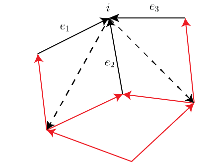
In the situation above, consider any two consecutive edges $e_{s}$ and $e_{s+1}$ (we make the convention that $e_{k+1}=e_{1}$ ). Because $S$ is a shrub (and thus has a root), we may continue these edges in $S$ until they meet, thus yielding paths

(3.14)			$\displaystyle p_{s}:j\rightarrow\dots\xrightarrow{e_{s}}i$
(3.15)			$\displaystyle p^{\prime}_{s}:j\rightarrow\dots\xrightarrow{e_{s+1}}i$

We may assume the paths $p_{s}$ and $p_{s}^{\prime}$ are simple, non-intersecting (except for the endpoints) and that the region $r_{s}$ of the plane between $p_{s}$ and $p_{s}^{\prime}$ is minimal with respect to inclusion; this guarantees the uniqueness of $p_{s},p_{s}^{\prime},r_{s}$ , since the intersection of two minimal regions thus constructed would yield an even smaller acceptable region. Because the vertex $i$ does not belong to the interior of the shrub, a single one of the regions $r_{s}$ does not contain the counterclockwise angle at $i$ between $e_{s}$ and $e_{s+1}$ . By relabeling the edges if necessary, we assume that the aforementioned region is $r_{k}$ . With this in mind, an index $s\in\{1,\dots,k-1\}$ is called

•

good if $p_{s}$ and $p^{\prime}_{s}$ are broken wheels, which are mirror images of each other
•

bad if there exist edges $i\xrightarrow{e}v\in p_{s}$ and $i\xrightarrow{e^{\prime}}v^{\prime}\in p^{\prime}_{s}$ with $v,v^{\prime}\neq j$ , such that the sub-regions of $r_{s}$ between $e$ and $p_{s}$ (respectively between $e^{\prime}$ and $p^{\prime}_{s}$ ) are faces

For example, both $s\in\{1,2\}$ in Figure 3 are good. However, in the picture on the left of Figure 4, $s=1$ is bad and $s=2$ is good. Meanwhile, we call the index $s=k$

•

good if there are no edges from $i$ to $S$ in the counterclockwise region from $e_{k}$ to $e_{1}$ (i.e. the region ${\mathbb{R}}^{2}\backslash r_{k}$ ); this is the case in Figure 3.
•

bad if there exists an edge from $i$ to $S$ in the region ${\mathbb{R}}^{2}\backslash r_{k}$ , which determines a face together with the other edges in $S$ and exactly one of the edges $e_{1}$ and $e_{k}$ ; this is the case in the picture on the right of Figure 4.

The following result will be proved in the Appendix.

Proposition 3.17.

For $i\notin S$ as above, every $s\in\{1,\dots,k\}$ is either good or bad.

3.18.

If $S$ is a shrub and $i\notin S$ , let $S+i$ denote the subgraph obtained from $S$ by adding the vertex $i$ and the edges from $S$ to $i$ (we assume such edges exist).

Definition 3.19.

In the situation above, we call $i$ addable to $S$ if all $s\in\{1,\dots,k\}$ are good, and non-addable to $S$ otherwise.

Figures 3 and 4 provide examples of addable and non-addable vertices. The terminology above is motivated by the following result, which will be proved in the Appendix.

Proposition 3.20.

Assume $S\subset\widetilde{Q}$ is a shrub and $i\notin S$ is a vertex. Then $S+i$ is a shrub if and only if $i$ is an addable vertex to $S$ .

The main distinction to us between addable and non-addable vertices is the following result, which will also be proved in the Appendix.

Proposition 3.21.

Assume $S\subset\widetilde{Q}$ is a shrub and $i\notin S$ is a vertex with $k>0$ edges from $S$ to $i$ . The maximal number of broken wheels in $S+i$ that all pass through $i$ and do not pairwise intersect at any other vertex is

\begin{cases}k-1&\text{if }i\text{ is addable to }S\\ \geq k&\text{otherwise}\end{cases}

3.22.

We are now ready to give the proof of Proposition 3.10. Since we are operating under Assumption 1.7, we will assume throughout the present Subsection that the edge parameters $t_{e}$ are non-zero complex numbers (i.e. abuse notation by writing $t_{e}$ instead of $\rho(t_{e})$ , where $\rho:{\mathbb{K}}\rightarrow{\mathbb{C}}$ is a field homomorphism). This assumption is merely cosmetic, as all our formulas are rational functions in the $t_{e}$ ’s.

Proof.

of Proposition 3.10: Let us consider any

\phi=\mathop{\sum_{i_{1},\dots,i_{n}\in I}}_{d_{1},\dots,d_{n}\in{\mathbb{Z}}}\text{coefficient}\cdot e_{i_{1},d_{1}}\dots e_{i_{n},d_{n}}\in K^{+}

and any $R\in\bm{\dot{}}{{\mathcal{S}}}^{-}$ . Our goal is to show that

(3.16)

\Big\langle\phi,R\Big\rangle=0

as this would imply the required $R\in{\mathcal{S}}^{-}$ . Recall from formula (2.8) that

(3.17)

\Big\langle e_{i_{1},d_{1}}\cdots e_{i_{n},d_{n}},R\Big\rangle=\int_{|z_{1}|\gg\dots\gg|z_{n}|}f(z_{1},\dots,z_{n})\prod_{a=1}^{n}Dz_{a}

where

(3.18)

f(z_{1},\dots,z_{n})=\frac{z_{1}^{d_{1}}\dots z_{n}^{d_{n}}R(z_{1},\dots,z_{n})}{\prod_{1\leq a<b\leq n}\zeta_{i_{b}i_{a}}\left(\frac{z_{b}}{z_{a}}\right)}

A labeling of a shrub $S\subset\widetilde{Q}$ will refer to a labeling of the $s$ vertices of $S$ by one of the variables $z_{a_{1}},\dots,z_{a_{s}}$ (for certain $a_{1}<\dots<a_{s}\in{\mathbb{N}}$ ) such that the increasing order of the indices of the variables refines the partial order on the vertices given by the shrub, i.e. $a_{x}<a_{x^{\prime}}$ if the corresponding vertices $i_{x},i_{x^{\prime}}\in S$ are connected in $S$ by a path going from $i_{x^{\prime}}$ to $i_{x}$ . In particular, the root of $S$ must be labeled by the variable $z_{a_{s}}$ . For every $x\in\{1,\dots,s-1\}$ , choose a path from the root $i_{s}$ to $i_{x}$

i_{s}\xrightarrow{\alpha}i_{s^{\prime}}\xrightarrow{\beta}\dots\xrightarrow{\omega}i_{x}

and define $q_{x}=t_{\alpha}t_{\beta}\dots t_{\omega}$ . Because such paths are unique up to removing cycles or replacing a broken wheel by its mirror image (according to Definition 1.5), and because such removals/replacements do not change the product of parameters along the path, the quantity $q_{x}$ does not depend on any choices made. An acceptable labeled shrub is one for which $|q_{x}|>1$ for all $x\in\{1,\dots,s-1\}$ (note that the situation of $p^{\prime}$ being the empty path in (1.2) precludes $|q_{x}|=1$ ).

Proposition 3.23.

For any labeled shrub $S$ and function $f$ as in (3.18) with at least as many variables as vertices of $S$ (corresponding to any $i\in I$ ), define

(3.19)

\mathop{\emph{Res}}_{S}f

as a function in $\{z_{a}\}_{a\notin\{a_{1},\dots,a_{s-1}\}}$ by the following iterated residue procedure.

At step number $x\in\{1,\dots,s-1\}$ , the variables $z_{a_{s-x+1}},\dots,z_{a_{s-1}}$ have all been specialized to $z_{a_{s}}$ times $q_{s-x+1},\dots,q_{s-1}$ , respectively. Upon this specialization, we claim that the rational function $f$ has at most a simple pole at

(3.20)

z_{a_{s-x}}=z_{a_{s}}q_{s-x}

Replace $f$ by its residue at the pole (3.20), and move on to step number $x+1$ .

Because one only encounters simple poles in the algorithm above, the value of (3.19) would not change if we replaced (in the recursive procedure of Proposition 3.23) the total order $a_{1}<\dots<a_{s}$ by any other total order refining the partial order on the vertices of the shrub.

Proof.

Consider the induced subgraph $S^{\prime}\subset S$ consisting of all vertices $>i:=i_{s-x}$ . It is easy to see that $S^{\prime}$ is a shrub and that $i$ is an addable vertex to $S^{\prime}$ . Therefore, we may assume that the there are $k>0$ edges

i_{b_{1}}\xrightarrow{e_{1}}i_{s-x},\dots,i_{b_{k}}\xrightarrow{e_{k}}i_{s-x}

from the shrub $S^{\prime}$ to the vertex $i$ , for certain $b_{1},\dots,b_{k}>s-x$ . Since these edges must be distributed as in Figure 3, the denominator of (3.18) includes the $k$ factors

1-\frac{z_{a_{b_{1}}}t_{e_{1}}}{z_{a_{s-x}}},\dots,1-\frac{z_{a_{b_{k}}}t_{e_{k}}}{z_{a_{s-x}}}

Once the variables $z_{a_{b_{1}}},\dots,z_{a_{b_{k}}}$ are specialized to $z_{a_{s}}$ times $q_{b_{1}},\dots,q_{b_{k}}$ , respectively, the fact that $q_{s-x}=q_{b_{1}}t_{e_{1}}=\dots=q_{b_{k}}t_{e_{k}}$ implies that the denominator of (3.18) will feature the factor

\left(1-\frac{z_{a_{s}}q_{s-x}}{z_{a_{s-x}}}\right)^{k}

Thus, to prove that the pole invoked in the statement of the Proposition is at most simple, we need to show that the numerator of (3.18) vanishes to order at least $k-1$ at the specialization (3.20). However, the numerator of $f$ vanishes whenever any subset of its variables are specialized according to (3.10) for any face $F$ . As there exist $k-1$ broken wheels whose only common vertex is $i=i_{s-x}$ (see Proposition 3.21), property (3.10) for the $k-1$ faces enclosed by said broken wheels implies that the numerator of $f$ vanishes to order $\geq k-1$ at the specialization (3.20). ⁹⁹ 9 In claiming the vanishing of the numerator of $f$ to order at least $k-1$ , we are invoking the fact that for any $k,\ell_{1},\dots,\ell_{k-1}\in{\mathbb{N}}$ , we have $\bigcap_{c=1}^{k-1}\left(x_{c}^{(1)},\dots,x_{c}^{(\ell_{c})}\right)=\left(x_{1}^{(\alpha_{1})}x_{2}^{(\alpha_{2})}\dots x_{k-1}^{(\alpha_{k-1})}\right)_{\alpha_{1}\in\{1,\dots,\ell_{1}\},\dots,\alpha_{k-1}\in\{1,\dots,\ell_{k-1}\}}$ in the ring of polynomials over distinct variables $\{x_{c}^{(1)},\dots,x_{c}^{(\ell_{c})}\}_{c\in\{1,\dots,k-1\}}$ .

∎

An $m$ -labeled shrubbery $\mathscr{S}$ is a disjoint union of labeled shrubs in $\widetilde{Q}$ (whose $n-m+1$ vertices are endowed with distinct labels among $z_{m},\dots,z_{n}$ ) such that the order of the indices of the variables refines the partial order on the vertices given by each constituent shrub of $\mathscr{S}$ . An $m$ -labeled shrubbery is called acceptable if all of its constituent shrubs are acceptable.

Claim 3.24.

For any $m\in\{1,\dots,n\}$ , consider

(3.21)

X_{m}=\sum^{m\text{-labeled acceptable}}_{\text{shrubberies }\mathscr{S}=S_{1}\sqcup\dots\sqcup S_{t}}\int_{|z_{1}|\gg\dots\gg|z_{m-1}|\gg|z_{r_{1}}|=\dots=|z_{r_{t}}|}\\ \mathop{\emph{Res}}_{S_{1}}\dots\mathop{\emph{Res}}_{S_{t}}f\prod_{a=1}^{m-1}Dz_{a}\prod_{u=1}^{t}Dz_{r_{u}}

where $z_{r_{1}},\dots,z_{r_{t}}$ are the labels of the roots of the shrubs $S_{1},\dots,S_{t}$ . Then we have

(3.22)

X_{m-1}=X_{m}

for all $m\in\{2,\dots,n\}$ .

Note that there are finitely many $m$ -labeled shrubberies, due to the fact that shrubs that only differ by a deck transformation of $\widetilde{Q}$ over $Q$ are identified. The purpose of assumption (1.2) is to ensure that the specialization of the rational function $f$ corresponding to the shrubbery $\mathscr{S}$ , which has linear factors of the form

1-\frac{z_{r_{u}}q_{x}t_{e}}{z_{r_{v}}q_{y}}

in the denominator (where $e$ is any edge from any vertex $i_{x}$ in the shrub $S_{u}$ to any vertex $i_{y}$ in the shrub $S_{v}$ ) has no poles on the circles $|z_{r_{u}}|=|z_{r_{v}}|$ themselves.

Proof.

To prove (3.22), one needs to move the contour of the variable $z_{m-1}$ toward the contours $|z_{r_{1}}|=\dots=|z_{r_{t}}|$ . If the former contour reaches the latter contours, this corresponds to adding the one-vertex shrub $\{i_{m-1}\}$ to the shrubbery $\mathscr{S}$ . Otherwise, the variable $z_{m-1}$ must be “caught” in one of the poles of the form

(3.23)

1-\frac{z_{b}t_{e}}{z_{m-1}}

for some $b>m-1$ and some edge $e=\overrightarrow{i_{b}i_{m-1}}$ . Assume $i_{b}$ belongs to one of the constituent shrubs $S_{u}\subset\mathscr{S}$ , and suppose there is a number $k>0$ of edges from the shrub $S_{u}$ to $i=i_{m-1}$ . Then we have one of the following three possibilities.

•

If the vertex $i$ is addable to $S_{u}$ as in Definition 3.19, then Proposition 3.20 implies that $S_{u}^{\prime}=S_{u}+i$ is a shrub. Thus, the operation

m\text{-labeled shrubbery }\mathscr{S}=S_{1}\sqcup\dots\sqcup S_{u}\sqcup\dots\sqcup S_{t}\leadsto\\ \leadsto(m-1)\text{-labeled shrubbery }\mathscr{S}^{\prime}=S_{1}\sqcup\dots\sqcup S^{\prime}_{u}\sqcup\dots\sqcup S_{t}

shows how to obtain $X_{m-1}$ by applying the contour moving procedure to $X_{m}$ (the fact that we only encounter acceptable shrubs is due to the fact that we move the contour of $z_{m-1}$ from infinity down to the contour of $z_{r_{u}}$ , but no further).

•

If the vertex $i$ is non-addable to $S_{u}$ , then Proposition 3.21 states that there exist $k$ broken wheels completely contained in $S_{u}+i$ that only intersect pairwise at the vertex $i$ . As we have seen at the end of the proof of Proposition 3.23, this means that the numerator of $f$ has enough factors to cancel the $k$ copies of the factor (3.23) from the denominator of $f$ . We conclude that non-addable vertices do not correspond to actual poles.
•

If the vertex $i$ is already in $S_{u}$ (say with label $z_{c}$ for some $c>m-1$ ), then the linear factor of $z_{m-1}-z_{c}$ in the denominator of

$\zeta_{i_{c}i_{m-1}}\left(\frac{z_{c}}{z_{m-1}}\right)$

allows the numerator of $f$ to annihilate the pole of the form (3.23).

∎

Repeated applications of Claim 3.24 imply the fact that $X_{1}=X_{n}$ . Since $X_{n}$ is the right-hand side of (3.17), we conclude that

(3.24)

\Big\langle e_{i_{1},d_{1}}\cdots e_{i_{n},d_{n}},R\Big\rangle=\sum^{1\text{-labeled acceptable}}_{\text{shrubberies }\mathscr{S}=S_{1}\sqcup\dots\sqcup S_{t}}\\ \int_{|z_{r_{1}}|=\dots=|z_{r_{t}}|}\mathop{\text{Res}}_{S_{1}}\dots\mathop{\text{Res}}_{S_{t}}\frac{z_{1}^{d_{1}}\dots z_{n}^{d_{n}}R(z_{1},\dots,z_{n})}{\prod_{1\leq a<b\leq n}\zeta_{i_{b}i_{a}}\left(\frac{z_{b}}{z_{a}}\right)}\prod_{u=1}^{t}Dz_{r_{u}}

The fact that all the contours coincide means that we can symmetrize the integrand (with respect to all variables $z_{1},\dots,z_{n}$ ) without changing the value of the integral

\Big\langle e_{i_{1},d_{1}}\cdots e_{i_{n},d_{n}},R\Big\rangle=\sum^{\text{fixed }1\text{-labeled acceptable}}_{\text{shrubberies }\bar{\mathscr{S}}=\bar{S}_{1}\sqcup\dots\sqcup\bar{S}_{t}}\\ \int_{|z_{r_{1}}|=\dots=|z_{r_{t}}|}\mathop{\text{Res}}_{\bar{S}_{1}}\dots\mathop{\text{Res}}_{\bar{S}_{t}}\text{ Sym}\left[\frac{z_{1}^{d_{1}}\dots z_{n}^{d_{n}}R(z_{1},\dots,z_{n})}{\prod_{1\leq a<b\leq n}\zeta_{i_{b}i_{a}}\left(\frac{z_{b}}{z_{a}}\right)}\right]\prod_{u=1}^{t}Dz_{r_{u}}

where the adjective “fixed” means that we are summing over a given 1-labeled acceptable shrubbery in every equivalence class given by permuting the labels on the vertices. Because of the identity

\widetilde{\Upsilon}^{+}(e_{i_{1},d_{1}}\cdots e_{i_{n},d_{n}})\stackrel{{\scriptstyle\eqref{eqn:shuf prod}}}{{=}}\textrm{Sym}\left[z_{1}^{d_{1}}\dots z_{n}^{d_{n}}\prod_{1\leq a<b\leq n}\zeta_{i_{a}i_{b}}\left(\frac{z_{a}}{z_{b}}\right)\right]

we conclude that

(3.25)

\Big\langle e_{i_{1},d_{1}}\cdots e_{i_{n},d_{n}},R\Big\rangle=\sum^{\text{fixed }1\text{-labeled acceptable}}_{\text{shrubberies }\bar{\mathscr{S}}=\bar{S}_{1}\sqcup\dots\sqcup\bar{S}_{t}}

\int_{|z_{r_{1}}|=\dots=|z_{r_{t}}|}\mathop{\text{Res}}_{\bar{S}_{1}}\dots\mathop{\text{Res}}_{\bar{S}_{t}}\frac{\widetilde{\Upsilon}^{+}(e_{i_{1},d_{1}}\cdots e_{i_{n},d_{n}})R(z_{1},\dots,z_{n})}{\prod_{1\leq a\neq b\leq n}\zeta_{i_{b}i_{a}}\left(\frac{z_{b}}{z_{a}}\right)}\prod_{u=1}^{t}Dz_{r_{u}}

We conclude that $\langle\phi,R\rangle$ is a linear functional of $\widetilde{\Upsilon}^{+}(\phi)$ . Since the latter expression is 0 due to the fact that $\phi\in K^{+}$ , we conclude the required formula (3.16).

∎

Note that (3.25) implies the following formula for the descended pairing (2.16), under the assumption that $Q$ is shrubby

(3.26)

\Big\langle R^{+},R^{-}\Big\rangle=\sum^{\text{fixed }1\text{-labeled acceptable}}_{\text{shrubberies }\bar{\mathscr{S}}=\bar{S}_{1}\sqcup\dots\sqcup\bar{S}_{t}}

\int_{|z_{r_{1}}|=\dots=|z_{r_{t}}|}\mathop{\text{Res}}_{\bar{S}_{1}}\dots\mathop{\text{Res}}_{\bar{S}_{t}}\text{ Sym}\left[\frac{R^{+}(z_{1},\dots,z_{n})R^{-}(z_{1},\dots,z_{n})}{\prod_{1\leq a\neq b\leq n}\zeta_{i_{b}i_{a}}\left(\frac{z_{b}}{z_{a}}\right)}\right]\prod_{u=1}^{t}Dz_{r_{u}}

for any $R^{\pm}\in{\mathcal{S}}^{\pm}$ of opposite degrees. Formula (3.26) shows that shrubberies are not just technical tools used in the proof of Proposition 3.10, but natural combinatorial objects which parameterize the summands in the formula for the pairing (2.16).

4. Appendix: the joys of gardening

In the present Section, we will motivate our notion of shrubby quivers by relating it with more traditional consistency conditions in the theory of brane tilings and dimer models. We also prove several technical results from Section 3.

4.1.

Let $Q$ denote a quiver in ${\mathbb{T}}^{2}$ , as in Definition 1.3, i.e. the faces of $Q$ are colored in blue/red such that any two faces which share an edge have different colors.

Definition 4.2.

A non-degenerate $R$ -charge (see for instance [7, 8]) is a function

R:E\rightarrow(0,1)

such that for any vertex $i$ and any face $F$ of the quiver $Q$ , we have

		$\displaystyle\sum_{e\text{ edge around }F}R(e)=2$
		$\displaystyle\sum_{e\text{ edge incident to }i}(1-R(e))=2$

¹⁰¹⁰ 10 Loops at

i

are counted twice in the formula above.

Geometrically, the properties above imply that the quiver $Q$ can be drawn on the torus so that all faces are polygons circumscribed in circles of the same radius, and the centers of these circles lie strictly inside the faces (the number $\pi R(e)$ is the central angle subtended by the chord $e$ in the aforementioned circles).

The existence of a non-degenerate $R$ -charge allows one to define a rhombus tiling of the torus, as follows. Draw the centers of the (circles circumscribing the) blue/red polygonal faces as blue/red bullets. Then the condition that the segments between the vertices and the bullets all have the same length means that ${\mathbb{T}}^{2}$ is tiled by rhombi. To recover the arrows in the quiver $Q$ from the rhombus tiling, one need only draw the diagonals between non-bullet vertices of the rhombi, and orient them so that they keep the blue/red bullets on the right/left (see Figure 5).

Recall the notion of shrubby quivers from Definition 1.5. Lemma 4.3 below is proved just like [7, Lemma 5.3.1] (note that the topology of shrubby quivers underlies the notion of $F$ -term equivalent paths, see [1, Definition 2.5] and [10, Condition 4.12]).

Lemma 4.3.

If there exists a non-degenerate $R$ -charge, then $Q$ is shrubby.

4.4.

In the remainder of the paper, we provide proofs of some technical results about shrubs and pre-shrubs, specifically Propositions 3.13, 3.15, 3.17, 3.20 and 3.21. Throughout the present Section, we assume $Q$ to be a shrubby quiver, with universal cover $\widetilde{Q}$ . All paths and cycles in a quiver are understood to be oriented.

Definition 4.5.

Given two paths $p$ and $p^{\prime}$ in $\widetilde{Q}$ with the same endpoints, we will write $r(p,p^{\prime})$ for the closed region inside ${\mathbb{R}}^{2}$ contained between $p$ and $p^{\prime}$ . The area of this region, denoted by $a(p,p^{\prime})\in{\mathbb{N}}$ , will refer to the number of faces contained inside $r(p,p^{\prime})$ . In particular, if $C$ is a cycle, we will write $r(C)$ and $a(C)$ for the closed region and area (respectively) contained inside $C$ .

Proof.

of Proposition 3.13: Assume for the purpose of contradiction that a pre-shrub $S$ contains a cycle, and let us fix such a cycle $C$ of minimal area (as in Definition 4.5). We must have $a(C)>2$ , since otherwise $C$ would be the boundary of a face, or the union of boundaries of two faces which meet at a single point, both situations being forbidden for pre-shrubs. Definition 1.5 for $p=C$ and $p^{\prime}=\text{trivial}$ implies that there exist two adjacent faces (as in Figure 2) for which e.g. the red path is completely contained in $C$ , and the red and blue regions are contained inside $r(C)$ . By the defining property of a pre-shrub, $S$ also contains the blue path. Thus, the cycle

C^{\prime}=C-\{\text{red path}\}+\{\text{blue path}\}

is contained in $S$ , and moreover $a(C^{\prime})=a(C)-2$ . This contradicts the minimality of the area of $C$ .

∎

Proof.

of Proposition 3.15: Assume that $e$ is an edge from vertex $i$ to vertex $i^{\prime}$ , where $i,i^{\prime}\in S$ but $e\not\subset S$ . By the very definition of the root $r$ of a shrub, there are paths from $r$ to $i$ and $i^{\prime}$ , respectively. Following the aforementioned paths until they first intersect, we conclude that there exist simple paths

		$\displaystyle p:j\rightarrow\dots\rightarrow i$
		$\displaystyle p^{\prime}:j\rightarrow\dots\rightarrow i^{\prime}$

with no vertices in common other than the source $j$ . We have three scenarios.

(1) If $j=i$ , then $e$ and $p^{\prime}$ are both paths from $i$ to $i^{\prime}$ . We may assume that $p^{\prime}$ is chosen such that $a(e,p^{\prime})$ is minimal. Definition 1.5 implies that $p^{\prime}$ contains a broken wheel $B$ (since $e$ consists of a single edge, it cannot contain a broken wheel). Since $S$ is a shrub, it therefore contains the mirror image $B^{\prime}$ of $B$ . Thus, if we modify $p^{\prime}$ by replacing its sub-path $B$ with $B^{\prime}$ , then we contradict the minimality of $a(e,p^{\prime})$ . We conclude that this scenario is impossible.

(2) If $j=i^{\prime}$ , then $C=p\cup e$ is a cycle, and we assume that $p$ is chosen so that $a(C)$ is minimal. If $a(C)=1$ then we are done (since $r(C)$ would be precisely the face that realizes $e$ as the interface of a broken wheel contained in $S$ ), so let us assume for the purpose of contradiction that $a(C)>1$ . Definition 1.5 implies that $C$ contains a broken wheel $B$ . There are two sub-cases.

•

If $e\not\subset B$ , then $S$ must also contain the mirror image $B^{\prime}$ of $B$ . If we modify $p$ by replacing its sub-path $B$ with $B^{\prime}$ , then we contradict the minimality of $a(C)$ .
•

If $e\subset B$ , then the interface $e^{\prime}$ of the broken wheel $B$ is an edge between two vertices of the shrub $S$ . If $e^{\prime}\subset S$ , then we contradict the minimality of $a(C)$ and the fact that $a(C)>1$ . If $e^{\prime}\not\subset S$ , then there is a sub-path of $p$ from the source to the tail of $e^{\prime}$ , and we are thus in the self-contradictory situation of item (1).

(3) If $j\notin\{i,i^{\prime}\}$ , then let us choose $p,p^{\prime},e$ such that $a(p\cup e,p^{\prime})$ is minimal. In this case, Definition 1.5 implies that one of $p\cup e$ or $p^{\prime}$ contains a broken wheel $B$ whose interface is contained in $r(p\cup e,p^{\prime})$ . If $B\subseteq p$ or $B\subseteq p^{\prime}$ , then we may modify the path $p$ or $p^{\prime}$ by replacing its sub-path $B$ with its mirror image, and contradict the minimality of $a(p\cup e,p^{\prime})$ . The only other possibility is that $e\subset B$ , in which case the interface of $B$ must be an edge $e^{\prime}:i^{\prime}\rightarrow v$ for some vertex $v\in p$ , as in Figure 6.

If $e^{\prime}\subset S$ , then concatenating $e^{\prime}$ with the sub-path of $p$ that goes from $v$ to $i$ puts us in the situation of item (2) above. Meanwhile, if $e^{\prime}\not\subset S$ and $v=j$ , the cycle formed by $p^{\prime}$ and $e^{\prime}$ also puts us in the situation of item (2); since $e^{\prime}$ must therefore be the interface of a broken wheel $B$ contained in $S$ , replacing $p^{\prime}$ by the mirror image $B^{\prime}$ of $B$ would contradict the minimality of $a(p\cup e,p^{\prime})$ . Finally, if $e^{\prime}\not\subset S$ and $v\neq j$ , then we note that

a(p^{\prime}\cup e^{\prime},p^{\prime\prime})<a(p\cup e,p^{\prime})

(where $p^{\prime\prime}$ is the sub-path of $p$ that goes from $j$ to $v$ ) contradicts the minimality of $a(p\cup e,p^{\prime})$ .

∎

Proof.

of Proposition 3.17: We will treat the case $s\in\{1,\dots,k-1\}$ , and leave the analogous case $s=k$ as an exercise to the reader. Consider the paths $p_{s}$ and $p^{\prime}_{s}$ of (3.14)–(3.15). Definition 1.5 states that one of these paths must contain a broken wheel $B$ ; without loss of generality, let us assume that $B\subseteq p_{s}$ . If $e_{s}$ were not part of $B$ , then we would be able to modify $p_{s}$ by replacing its sub-path $B$ with its mirror image $B^{\prime}$ , and thus contradict the minimality of $a(p_{s},p^{\prime}_{s})$ . Therefore, we may assume that $e_{s}$ is part of $B$ , and thus there exists $v\in p_{s}$ and an edge

i\xrightarrow{e}v

such that the region bounded by $e$ and $p_{s}$ is a face. If $v=j$ , then the index $s$ is good (since the whole of $p_{s}$ is the sought-for broken wheel, and its mirror image must coincide with $p^{\prime}_{s}$ by minimality). Otherwise $v\neq j$ and let us consider the paths

		$\displaystyle\tilde{p}_{s}:j\rightarrow\dots\rightarrow v$
		$\displaystyle\tilde{p}^{\prime}_{s}:j\rightarrow\dots\xrightarrow{e_{s+1}}i\xrightarrow{e}v$

as in Figure 7.

Definition 1.5 implies that one of the paths $\tilde{p}_{s}$ and $\tilde{p}^{\prime}_{s}$ must contain a broken wheel $\tilde{B}$ . If $\tilde{B}$ did not contain the edges $e_{s+1}$ or $e$ , then we could contradict the minimality of $a(p_{s},p^{\prime}_{s})$ by replacing $\tilde{B}$ with its mirror image $\tilde{B}^{\prime}$ . We are left only with the possibility of $\tilde{B}$ containing the edges $e_{s+1}$ or $e$ , and we have two cases

•

If the interface $e^{\prime}$ of $\tilde{B}$ is an edge from $i$ to some $v^{\prime}\in p^{\prime}_{s}$ , then we assume $v^{\prime}\neq j$ (as the case $v^{\prime}=j$ can be treated like the case $v=j$ was treated above). We are thus in the situation of Figure 7 and the index $s$ is bad.
•

If the interface $e^{\prime}$ of $\tilde{B}$ is an edge from $v$ to some vertex $v^{\prime}\in p^{\prime}_{s}\backslash\{i\}$ , then we are in the situation of Figure 8. We have two sub-cases. If $e^{\prime}\subset S$ , then we contradict the minimality of $a(p_{s},p^{\prime}_{s})$ . On the other hand, if $e^{\prime}\not\subset S$ , then Proposition 3.15 forces $e^{\prime}$ to be the interface of a broken wheel $\bar{B}\subset S$ . The paths

$v^{\prime}\xrightarrow{\bar{B}}v\rightarrow\dots\xrightarrow{e_{s}}i$

and $v^{\prime}\rightarrow\dots\xrightarrow{e_{s+1}}i$ contradict the minimality of $a(p_{s},p^{\prime}_{s})$ .

Figure 8. An impossible case.

∎

Proof.

of Proposition 3.20: If $i$ is not an addable vertex, there must exist a bad index $s\in\{1,\dots,k\}$ , i.e. either the situation of $s=1$ in the picture on the left of Figure 4 or the situation of $s=3$ in the picture on the right of Figure 4. In both of these cases, one can see a broken wheel in $S+i$ whose mirror image is not contained in $S+i$ , thus precluding $S+i$ from being a shrub.

Conversely, suppose that $i$ is an addable vertex, and let us show that $S+i$ is a shrub. It is clear that $i$ can be reached via a path from the root, and that there are no vertices $\notin S+i$ inside the polygonal regions incident to $i$ in Figure 3.

Assume for the purpose of contradiction that $S+i$ contains the entire boundary of a face. Since $S$ cannot contain the entire boundary of a face (as $S$ is a shrub), then the boundary in question must involve the vertex $i$ . However, this would require an edge from $i$ to a vertex of $S$ , which is not in $S+i$ by assumption.

Now let us assume that $S+i$ contains a broken wheel $B$ , and let us show that it also contains its mirror image. Since $S$ is already a shrub, we may assume that the broken wheel $B$ involves the vertex $i$ . By the definition of an addable vertex, all possible edges between $i$ and $S$ are as in Figure 3. Thus, the interface of the broken wheel $B$ must be one of the dotted edges in Figure 3, and it is clear that the mirror image of $B$ is also contained in $S+i$ .

∎

Proof.

of Proposition 3.21: If $i$ is addable to $S$ , then all $s\in\{1,\dots,k\}$ are good. Therefore, there exist only $k-1$ outgoing edges from $i$ to $S$ , and they are arrayed as in Figure 3. Among any family of faces passing through $i$ and without other pairwise intersections, no two faces can pass through the same outgoing edge, so the cardinality of the family is at most $k-1$ . It is also easy to see that this maximum can be achieved, by taking for instance the collection of faces incident to $e_{1},\dots,e_{k-1}$ in clockwise order around $i$ .

If $i$ is non-addable to $S$ , then there exists a bad index $s$ . Assume first that $s\in\{1,\dots,k-1\}$ , e.g. we are in the situation of $s=1$ in the picture on the left of Figure 4. The two faces contained in the region $r_{s}$ , together with the faces incident to $e_{1},\dots,e_{s-1}$ in clockwise order around $i$ , and the faces incident to $e_{s+2},\dots,e_{k}$ in counterclockwise order around $i$ , yield altogether a family of $k$ faces which only pairwise intersect at $i$ .

If $s=k$ is a bad index, then we are in the situation in the picture on the right of Figure 4. Without loss of generality, let us assume that there is a face incident to $e_{k}$ in clockwise order around $i$ . Then this face together with the faces incident to $e_{1},\dots,e_{k-1}$ in clockwise order around $i$ , yield the required family of $k$ faces which only pairwise intersect at $i$ .

∎

References

[1] Davison B., Consistency conditions for brane tilings, Journal of Algebra, Volume 338, Issue 1 (2011), Pages 1-23
[2] Enriquez B., On correlation functions of Drinfeld currents and shuffle algebras, Transform. Groups 5 (2000), no. 2, 111–120.
[3] Feigin B., Odesskii A., Quantized moduli spaces of the bundles on the elliptic curve and their applications, Integrable structures of exactly solvable two-dimensional models of quantum field theory (Kiev, 2000), 123–137, NATO Sci. Ser. II Math. Phys. Chem., 35, Kluwer Acad. Publ., Dordrecht, 2001.
[4] Galakhov D., Li W., Yamazaki M., Toroidal and elliptic quiver BPS algebras and beyond, J. High Energy Phys., 24 (2022)
[5] Galakhov D., Li W., Yamazaki M., Gauge/Bethe correspondence from quiver BPS algebras, J. High Energy Phys., 119 (2022)
[6] Kontsevich M., Soibelman Y., Cohomological Hall algebra, exponential Hodge structures and motivic Donaldson-Thomas invariants, Commun. Number Theory Phys. 5 (2011), no. 2, 231–352
[7] Hanany A., Herzog C., Vegh D., Brane Tilings and Exceptional Collections, J. High Energ. Phys. 27 (2006)
[8] Hanany A., Vegh D., Quivers, Tilings, Branes and Rhombi, J. High Energ. Phys. 10 (2007)
[9] Li W., Yamazaki M., Quiver Yangian from crystal melting, J. High Energ. Phys. 35 (2020)
[10] Mozgovoy S., Reineke M., On the noncommutative Donaldson-Thomas invariants arising from brane tilings, Adv. Math. Volume 223, Issue 5 (2010), Pages 1521-1544
[11] Negu

t

,

A., Quantum loop groups for arbitrary quivers, ar $\chi$ iv:2209.09089
[12] Negu

t

,

A., Quantum loop groups for symmetric Cartan matrices, ar $\chi$ iv:2207.05504
[13] Noshita, G., Watanabe, A. A note on quiver quantum toroidal algebra, J. High Energ. Phys. 2022, 11 (2022)
[14] Noshita, G., Watanabe, A. Shifted Quiver Quantum Toroidal Algebra and Subcrystal Representations, J. High Energ. Phys., 122 (2022)
[15] Pădurariu T., $K$ -theoretic Hall algebras of quivers with potential as Hopf algebras, Int. Math. Res. Not. (2022)
[16] Rapcak M., Soibelman Y., Yang Y., Zhao G., Cohomological Hall algebras, vertex algebras and instantons, Comm. Math. Phys., 376(3):1803–1873, 2020.
[17] Tsymbaliuk A., The affine Yangian of $\widehat{{\mathfrak{gl}}}_{1}$ revisited, Adv. Math., Volume 304, 2017, 583–645.