Simultaneous Fermion and Exciton Condensations from a Model Hamiltonian

Superconductivity results from the condensation of bosonic fermion-fermion pairs Bose and Einstein 1924; Einstein 1924; Bardeen et al. 1957; Anderson 2013 into a single geminal—a two-fermion function directly analogous to the one-fermion orbital Yang 1962; Coleman 1963a; Sasaki 1965; Raeber and Mazziotti 2015; Surján 1999; Shull 1959—at temperatures below a certain critical temperature. This condensation of fermion-pairs results in the superfluidity (i.e., frictionless flow) of the constituent particle-particle pairs London 1938; Tisza 1947; Bardeen et al. 1957; Anderson 2013; if the fermionic pairs are composed of electrons (i.e., Cooper pairs), then these superfluid electron-electron pairs demonstrate superconductivity.

As was first demonstrated by Yang Yang 1962 and Sasaki Sasaki 1965, a computational signature of such superconducting states is a large eigenvalue in the particle-particle reduced density matrix (2-RDM), whose elements are given by

where $|\Psi\rangle$ is an $N$-fermion wavefunction and where $\hat{a}_{i}^{\dagger}$ and $\hat{a}_{i}$ are fermionic creation and annihilation operators for orbital $i$, respectively. As eigenvalues of the 2-RDM can be interpreted as the occupations of the two-fermion geminals Coleman 1963b, when the largest eigenvalue of the 2-RDM—the signature of particle-particle condensation, represented by $\lambda_{D}$—exceeds the Pauli-like limit of one ($\lambda_{D}>1$), multiple fermion-fermion pairs occupy a single geminal and hence superconducting character is observed. This signature is known to directly probe the presence and extent of non-classical (off-diagonal) long-range order Raeber and Mazziotti 2015. (See the Appendix for more details on how the signature of superconductivity, $\lambda_{D}$, was computed.)

The Pairing-Force (PF) model Richardson 1963a; Richardson 1963b; Richardson and Sherman 1964; Richardson 1965—also called the Standard Reduced Bardeen-Cooper-Schrieffer (BCS) model Bardeen et al. 1957; von Delft et al. 1996; Khamoshi et al. 2020—is known to exhibit superconducting character in the strong correlation limit and hence achieve a large $\lambda_{D}$. The Hamiltonian for the PF model is given in second quantization by

where $p$ is a quantum number that represents a pair of orbitals denoted as $p,\uparrow$ and $p,\downarrow$ with the same energy, where the energies ($\epsilon_{p}$) are considered to be known, and where the parameter $G$ is a constant that tunes the strength of the pairwise interactions. Note that in the limit of strong correlation ($G>>\epsilon_{p}$), maximal superconducting character—$\lambda_{D}=\frac{N}{2}\left(1-\frac{N-2}{r}\right)$ Coleman 1963a; Coleman 1963b—is observed.

Directly analogous to superconductivity resulting from bosonic particle-particle pairs condensing into a single particle-particle function, exciton condensation results from the condensation of particle-hole pairs (i.e., excitons) into a single particle-hole function below a certain critical temperature, which results in the superfluidity of the excitons Fil and Shevchenko 2018; Keldysh 2017. Exciton condensates, while difficult to realize experimentally, have been observed in systems composed of polaritons (excitons coupled to photons) Kasprzak et al. 2006; Fuhrer and Hamilton 2016; Pannir-Sivajothi et al. 2021 and in two-dimensional structures such as semiconductors Butov et al. 1994, graphene bilayers Liu et al. 2017; Min et al. 2008; Cao et al. 2018, and van der Waals heterostructures Sigl et al. 2020; Wang et al. 2019; Fogler et al. 2014; Kogar et al. 2017.

The signature of exciton condensation—denoted as $\lambda_{G}$—is similarly analogous to that for fermion-pair condensation; the presence and extent of exciton condensate character can be measured from the largest eigenvalue of a modified particle-hole reduced density matrix given by Safaei and Mazziotti 2018; Garrod and Rosina 1969; Kohn and Sherrington 1970

where ${}^{1}D$ is the one-fermion reduced density matrix (1-RDM). Note that this modification removes the extraneous large eigenvalue from a ground-state-to-ground-state transition such that a signature above one ($\lambda_{G}>1$) is indicative of exciton condensation. (See the Appendix for more details on how the signature of exciton condensation, $\lambda_{G}$ was computed.) This computational signature has been utilized to study exciton condensation is possible in quantum and molecular systems Safaei and Mazziotti 2018; Sager et al. 2020b; Sager et al. 2020a; Sager and Mazziotti 2021; Schouten et al. 2021.

One model known to achieve a large $\lambda_{G}$ value and hence exhibit exciton condensate character in the limit of a large correlation is the Lipkin quasispin model Lipkin et al. 1965; Pérez et al. 1988; Debergh and Stancu 2001; Mazziotti 2004; Heiss 2006; Castaños et al. 2006; Co’ and De Leo 2018. The $N$-fermion Lipkin quasispin model consists of two energy levels $\left\{-\frac{\epsilon}{2},\frac{\epsilon}{2}\right\}$, each containing $N$ energetically-degenerate states. The second-quantized Hamiltonian can be expressed as Mazziotti 2004

where $\sigma=\pm 1$ and $p=1,2,\dots,N$ are quantum numbers that completely characterize the system in which $p$ describes the site number labelling the $N$ states in a given level and $\sigma$ represents the upper ($+1$) or lower ($-1$) energy levels, respectively. Note that in this model, the $\lambda$ term allows for double excitations and de-excitations, and the $\gamma$ term allows for a single particle to be scattered up while another is simultaneously scattered down; as a result, in the Lipkin model, only even excitations are allowed, and only one particle may occupy a given site (i.e., have a specific quantum number $p$) such that each site in the lower level is particle-hole paired with the corresponding site in the upper level. By having the terms correlating orbitals in the Hamiltonian ($\lambda,\gamma$) be sufficiently larger than the energy term (i.e., in the limit of high correlation), maximal exciton condensation—$\lambda_{G}=\frac{N}{2}$ Garrod and Rosina 1969—can be obtained for $\lambda=\gamma$.

A fermion-exciton condensate is a single quantum state that simultaneously demonstrates character of superconductivity and exciton condensation, i.e., both signatures of condensation—the largest eigenvalue of the particle-particle RDM (Eq. (1)) and the largest eigenvalue of the modified particle-hole RDM (Eq. (3))—are simultaneously large ($\lambda_{D},\lambda_{G}>1$). Sager et al. 2020b.

To gain insight into such fermion-exciton condensates, here we propose a model system that is capable of demonstrating simultaneous fermion-pair and exciton condensate character. In this model, we introduce the pairwise interaction from the Pairing-Force model into the scaffolding of the Lipkin model; thus, the model keeps the structure of the Lipkin model in which $N$ particles occupy two $N$-degenerate energy levels ($-\frac{\epsilon}{2}$ and $\frac{\epsilon}{2}$) with allowed double excitations on two sites ($\lambda$) and simultaneous scattering of a particle up on one site and down on another ($\gamma$)—where Lipkin-like sites are now given as orbitals $p$ and $p+N$; however, we additionally pair adjacent orbitals—orbitals $2j-1$ and $2j$ for $j\in\{1,2,\dots,N\}$—via the PF parameter, $G$. (See Fig. 2.) The Hamiltonian for this model is thus given by

in second quantization, with a given set of parameters ($\epsilon,\lambda,\gamma,G$) directly determining the extent of fermion-pair and exciton condensation ($\lambda_{D}$ and $\lambda_{G}$, respectively) of the ground state corresponding to this model Hamiltonian.

While this model Hamiltonian is not the first to combine the pairwise interaction from the Pairing-Force model with the Lipkin model, the model Hamiltonian introduced by Plastino and coworkers causes direct competition between particle-particle and particle-hole correlations and hence proves incapable of demonstrating a fermion-exciton condensate phase (see Appendix B) Cambiaggio and Plastino 1978; Pennini and Plastino 2018; Plastino et al. 2021. Conversely, due to our introduction of the Pairing-Force interactions between adjacent orbitals instead of orbitals in the same Lipkin-like site, particle-particle and particle hole pairing can coexist and hence fermion-pair-exciton (FEC) states can be achieved as is shown in the results that follow.

As the authors have previously demonstrated Sager et al. 2020b, a system with as few as $N=4$ particles in $r=8$ orbitals can support formation of a fermion-exciton condensate. As such, we first fully explore such a minimalistic FEC system. The ground state of the FEC Hamiltonian that we have introduced—Equation (5)—for four particles has contributions from only ten of the seventy ($rCN$) possible configurations. Of these ten basis states, there are only five distinct classes composed of degenerate orientations—see Fig. 3—that allow for the direct computation of a matrix-form of the Hamiltonian in a minimal basis state. The five basis states are defined by three quantum numbers, $x,y,bool$, where the first indicates the number of particles excited to the upper energy level ($x$), the second indicates the number of BCS-like pairs (number of times both $2j-1$ and $2j$ are occupied, $y$), and the third is a boolean that indicates whether the configuration is “Lipkin”-like in the regard that no two orbitals representing a “Lipkin” site (denoted as $p$ and $p+N$, see the blue arrow in Fig. 3) are dually occupied or dually unoccupied.

Utilizing the basis shown in Fig. 3—$|0,2,T\rangle,\ |2,2,F\rangle,\ |2,2,T\rangle,\ |2,0,T\rangle,$ and $|4,2,T\rangle$—the Hamiltonian from Eq. (5) can be represented by

where each term—corresponding to the interaction between two classes of basis states, $|i\rangle$ and $|j\rangle$—is obtained from programmatically generating all sets of second-quantization creation and annihilation operators in Eq. (5), taking the expectation value for each combination of pairs of configurations in classes $|i\rangle$ and $|j\rangle$, summing the results, and normalizing by dividing by the square root of the number of configurations for both $|i\rangle$ and $|j\rangle$. For example, if $|i\rangle=|2,2,F\rangle=\left(|1,2,5,6\rangle+|3,4,7,8\rangle\right)/\sqrt{2}$ and $|j\rangle=|2,2,T\rangle=\left(|1,2,7,8\rangle+|3,4,5,6\rangle\right)/\sqrt{2}$, the Hamiltonian term would be given by

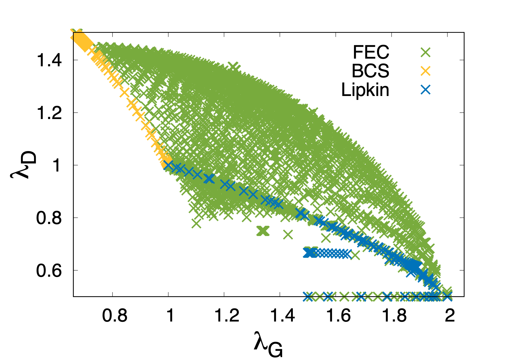
Fig. 4a scans over the signatures of condensation—$\lambda_{D}$ and $\lambda_{G}$—for the ground state of the Hamiltonian in Eq. (6) by systematically varying the parameters $\epsilon$, $\lambda$, $\gamma$, and $G$ where the yellow BCS x’s represent ground states in which the PF Hamiltonian is implemented (i.e., $\lambda=\gamma=0$), the blue Lipkin x’s represent states in which the Lipkin Hamiltonian is implemented (i.e., $G=0$), and where the green FEC x’s represent states with character of both PF and Lipkin Hamiltonians. As this figure demonstrates, the largest degree of superconducting character (the largest $\lambda_{D}$) is indeed observed in the BCS limit of the FEC Hamiltonian (when $G>>\epsilon,\ \lambda=\gamma\approx 0$), and the largest degree of exciton condensate character (the largest $\lambda_{G}$) is observed in the Lipkin limit of the FEC Hamiltonian ($\lambda\approx\gamma>>\epsilon,\ G\approx 0$). However, neither the BCS nor Lipkin limits of the Hamiltonian is capable of demonstrating a dual fermion-exciton condensate as $\lambda_{D}$ and $\lambda_{G}$ only simultaneously exceed the Pauli-like limit of one when the full FEC Hamiltonian from Eq. (5) is implemented including both BCS-like ($G$) and Lipkin-like ($\lambda,\gamma$) terms.

Our model FEC Hamiltonian, however, is capable of demonstrating a wide variety of dual condensate character as a variety of input parameters lead to ground state configurations in which both $\lambda_{G}$ and $\lambda_{D}$ simultaneously exceed one. Additionally, the $\lambda_{D}$ and $\lambda_{G}$ values obtained by scanning over the Hamiltonian parameters (in Fig. 4a) demonstrate an elliptic nature consistent with the convex nature of 2-RDMs projected onto a two-dimensional space Schwerdtfeger and Mazziotti 2009; Gidofalvi and Mazziotti 2006; Zauner et al. 2016 that matches predictions for a FEC that these authors first presented in Ref. Sager et al. 2020b. This elliptic boundary as well as the density of points in the zone corresponding to fermion-exciton condensate character indicate that the FEC model Hamiltonian introduced here is capable of spanning the entirety of the FEC region of $\lambda_{D}$ versus $\lambda_{G}$ space (i.e., $\lambda_{D},\lambda_{G}>1$).

In Ref. Sager et al. 2020b, these authors theoretically establish that in the thermodynamic limit, a possible wavefunction demonstrating fermion-exciton condensation can be obtained by entangling wavefunctions that separately demonstrate superconducting character ($|\Psi_{D}\rangle$ with large $\lambda_{D}$) and exciton condensate character ($|\Psi_{G}\rangle$ with large $\lambda_{G}$) according to

where $\Delta=2\langle\Psi_{D}|\Psi_{G}\rangle$. In Fig. 5 occupation probabilities for each of the five classes of basis states consistent with the $N,r=4,8$ FEC Hamiltonian that contribute to a BCS wavefunction (yellow, $\epsilon,\lambda,\gamma,G=0,0,0,0.7$, $\lambda_{D}=1.50$, $\lambda_{G}=0.67$), a Lipkin wavefunction (blue, $\epsilon,\lambda,\gamma,G=0,-0.5,-0.5,0$, $\lambda_{D}=0.50$, $\lambda_{G}=2.00$), and a FEC wavefunction (green, $\epsilon,\lambda,\gamma,G=0,-0.5,-0.5,0.7$, $\lambda_{D}=1.31$, $\lambda_{G}=1.32$) are given. From this data, it can be observed that the FEC wavefunction does indeed appear to be an entanglement of the individual BCS and Lipkin wavefunctions for the case of $N=4$; this is consistent with the theoretical result in the thermodynamic limit.

In order to observe trends related to system size, we employ the methodologies used to explore the $N,r=4,8$ model system and extrapolate to systems composed of $N=6,8,10$ particles in $r=12,16,20$ orbitals. Figures summarizing the signatures of superconducting character ($\lambda_{D}$) and exciton condensate character ($\lambda_{G}$) obtained for the ground state wavefunctions of these larger model Hamiltonians can be seen in Figs. 4b-4d. Similar to the results from the $N=4$ data, elliptic fits spanning the maximal signature of superconducting character observed for the BCS wavefunction to the maximal signature of exciton condensate character for the Lipkin wavefunction with a large variety of parameters supporting dual fermion-exciton condensation. Note that as the size of the system increases from $N=6$ to $N=8$ to $N=10$, the number of classes of degenerate, non-zero basis states as well as the number of basis states composing each class increase from $8$ classes with a total of $44$ non-zero basis states to $14$ classes with a total of $230$ non-zero basis states to $20$ classes with a total of $1212$ non-zero basis states. As such, the relative sparsity of the computations in $\lambda_{D}$ versus $\lambda_{G}$ as system size is increased is due to fewer computations being run with larger increments between each of the parameters as they are varied.

To demonstrate how the classes of non-zero basis states vary as system size is increased, Fig. 6—which shows the occupation probabilities for each of the fourteen classes of basis states consistent with the $N,r=8,16$ FEC Hamiltonian that contribute to a BCS wavefunction (yellow, $\epsilon,\lambda,\gamma,G=0,0,0,0.9$, $\lambda_{D}=2.50$, $\lambda_{G}=0.57$), a Lipkin wavefunction (blue, $\epsilon,\lambda,\gamma,G=0,-0.5,-0.5,0$, $\lambda_{D}=0.50$, $\lambda_{G}=4.00$), and a FEC wavefunction (green, $\epsilon,\lambda,\gamma,G=0,-0.5,-0.5,0.9$, $\lambda_{D}=2.06$, $\lambda_{G}=1.87$)—is included. Note that due to an increase in the possible complexity, two more quantum numbers are added to describe a few of the classes of basis states; specifically, $\zeta$ and $\tau$ are added to $x,y,bool,\zeta,\tau$ where $\zeta$ corresponds to the number of times BCS-like pairs are “stacked” into the same site such that orbitals $2j-1$, $2j$, $2j-1+N$, and $2j+N$ are all occupied and where $\tau$ corresponds to the number of diagonal configurations in which either $2j-1/2j+N$ or $2j-1+N/2j$ are both occupied where $2j-1$ and $2j$ are adjacent, BCS-paired orbitals. A few configurations with the necessary quantum numbers specified for $N=8$ are included in Fig. 7.

As can be seen from Fig. 6, the groundstate wavefunction for the $N=8$ FEC Hamiltonian no longer simply contains elements of the BCS wavefunction and the Lipkin wavefunction naively entangled together. Specifically, while the $|4,4,F,1,2\rangle$ class of basis states does include BCS-paired particles (see Fig. 7), it does not include the maximal number of BCS-paired particles, which appears to be a necessary condition for non-zero occupation of the ground state for the BCS Hamiltonian. However, this class of basis states can interact with other BCS-like and Lipkin-like classes of basis states. Explicitly, $|4,4,F,1,2\rangle$ interacts with $|2,4,F\rangle$ via $\frac{\lambda}{2}\hat{a}^{\dagger}_{p}\hat{a}^{\dagger}_{q}\hat{a}_{q+N}\hat{a}_{p+N}$; $|4,4,F,1\rangle$ via $\frac{\lambda}{2}\hat{a}^{\dagger}_{p}\hat{a}^{\dagger}_{q+N}\hat{a}_{q}\hat{a}_{p+N}$; $|6,4,F\rangle$ via $\frac{\lambda}{2}\hat{a}^{\dagger}_{p+N}\hat{a}^{\dagger}_{q+N}\hat{a}_{q}\hat{a}_{p}$; and $|2,2,T\rangle$ via $-G\hat{a}^{\dagger}_{2j-1}\hat{a}^{\dagger}_{2j}\hat{a}_{2k}\hat{a}_{2k-1}$, which does further entangle the Lipkin-like configurations and BCS-like configurations in a non-trivial manner. As such, while the interaction between the BCS-like classes of basis states and Lipkin-like classes of basis states in the formation of the FEC ground state wavefunction is not as clear-cut or simple as in the $N=4$ case, the $N=8$ FEC wavefunction is still an entanglement of BCS-like and Lipkin-like terms.

A representative configuration as well as the relevant quantum numbers for all classes of basis states for the $N=6$, $N=8$, and $N=12$ FEC Hamiltonians is given in the Supplemental Information.

References

- Rabe and Waghmare (1994) K. Rabe and U. Waghmare, First-principles model hamiltonians for ferroelectric phase transitions, Ferroelectrics 151, 59 (1994), cited By 6.
- Ostilli and Presilla (2006) M. Ostilli and C. Presilla, The exact ground state for a class of matrix hamiltonian models: Quantum phase transition and universality in the thermodynamic limit, J. Stat. Mech. Theory Exp. 10.1088/1742-5468/2006/11/P11012 (2006), cited By 5.
- Debnath et al. (2021) D. Debnath, M. Malik, and A. Chatterjee, A semi exact solution for a metallic phase in a holstein-hubbard chain at half filling with gaussian anharmonic phonons, Sci. Rep. 11, 10.1038/s41598-021-91604-6 (2021), cited By 0.
- Cai et al. (2021) M.-L. Cai, Z.-D. Liu, W.-D. Zhao, Y.-K. Wu, Q.-X. Mei, Y. Jiang, L. He, X. Zhang, Z.-C. Zhou, and L.-M. Duan, Observation of a quantum phase transition in the quantum rabi model with a single trapped ion, Nat. Commun. 12, 10.1038/s41467-021-21425-8 (2021), cited By 1.
- Farías and Davis (2021) C. Farías and S. Davis, Multiple metastable states in an off-lattice potts model, Physica A 581, 10.1016/j.physa.2021.126215 (2021), cited By 0.
- Richardson (1963a) R. Richardson, A restricted class of exact eigenstates of the pairing-force Hamiltonian, Phys. Lett. 3, 277 (1963a).
- Richardson (1963b) R. Richardson, Application to the exact theory of the pairing model to some even isotopes of lead, Phys. Lett. A 5, 82 (1963b), cited By 80.
- Richardson and Sherman (1964) R. Richardson and N. Sherman, Exact eigenstates of the pairing-force Hamiltonian, Nucl. Phys. 52, 221 (1964), cited By 366.
- Richardson (1965) R. W. Richardson, Exact eigenstates of the pairing-force hamiltonian. ii, J. Math. Phys. 6, 1034 (1965).
- Bardeen et al. (1957) J. Bardeen, L. N. Cooper, and J. R. Schrieffer, Theory of superconductivity, Phys. Rev. 108, 1175 (1957).
- Korenblit et al. (2012) S. Korenblit, D. Kafri, W. Campbell, R. Islam, E. Edwards, Z.-X. Gong, G.-D. Lin, L.-M. Duan, J. Kim, K. Kim, and C. Monroe, Quantum simulation of spin models on an arbitrary lattice with trapped ions, New J. Phys. 14, 10.1088/1367-2630/14/9/095024 (2012), cited By 77.
- Hernández-Sarria et al. (2015) J. Hernández-Sarria, A. Argüelles, and K. Rodríguez, Quantum magnetism in spin-3/2 chains (2015) cited By 0.
- Farnell et al. (2019) D. Farnell, R. Bishop, and J. Richter, Non-coplanar model states in quantum magnetism applications of the high-order coupled cluster method, J. Stat. Phys. 176, 180 (2019), cited By 0.
- Środa et al. (2021) M. Środa, E. Dagotto, and J. Herbrych, Quantum magnetism of iron-based ladders: Blocks, spirals, and spin flux, Phys. Rev. B 104, 10.1103/PhysRevB.104.045128 (2021), cited By 0.
- Lipkin et al. (1965) H. J. Lipkin, N. Meshkov, and A. J. Glick, Validity of many-body approximation methods for a solvable model: (I.) Exact solutions and perturbation theory, Nuclear Physics A 62, 188 (1965).
- Pérez et al. (1988) R. Pérez, M. C. Cambiaggio, and J. P. Vary, t expansion and the Lipkin model, Phys. Rev. C 37, 2194 (1988).
- Debergh and Stancu (2001) N. Debergh and F. L. Stancu, On the exact solutions of the lipkin-meshkov-glick model, Journal of Physics A: Mathematical and General 34, 3265 (2001).
- Mazziotti (2004) D. A. Mazziotti, Exactness of wave functions from two-body exponential transformations in many-body quantum theory, Phys. Rev. A 69, 012507 (2004).
- Heiss (2006) W. D. Heiss, On the thermodynamic limit of the lipkin model, Journal of Physics A: Mathematical and General 39, 10081 (2006).
- Castaños et al. (2006) O. Castaños, R. López-Peña, J. G. Hirsch, and E. López-Moreno, Classical and quantum phase transitions in the lipkin-meshkov-glick model, Phys. Rev. B 74, 104118 (2006).
- Co’ and De Leo (2018) G. Co’ and S. De Leo, Analytical and numerical analysis of the complete lipkin–meshkov–glick hamiltonian, International Journal of Modern Physics E 27, 1850039 (2018), https://doi.org/10.1142/S0218301318500398 .
- Cioslowski et al. (2000) J. Cioslowski, R. Erdahl, and B. Jin, On calculating approximate and exact density matrices, in Many-electron densities and reduced density matrices (Kluwer Academic/Plenum Publishers, 2000).
- Xia et al. (2018) R. Xia, T. Bian, and S. Kais, Electronic structure calculations and the Ising Hamiltonian, J. Phys. Chem. B 122, 3384 (2018), pMID: 29099600, https://doi.org/10.1021/acs.jpcb.7b10371 .
- Chu et al. (2020) A. Chu, J. Will, J. Arlt, C. Klempt, and A. Rey, Simulation of xxz spin models using sideband transitions in trapped bosonic gases, Phys. Rev. Lett. 125, 10.1103/PhysRevLett.125.240504 (2020), cited By 2.
- Khamoshi et al. (2021) A. Khamoshi, F. Evangelista, and G. Scuseria, Correlating agp on a quantum computer, Quantum Sci. Technol. 6, 10.1088/2058-9565/abc1bb (2021), cited By 5.
- Hu et al. (2012) Z.-X. Hu, Z. Papić, S. Johri, R. Bhatt, and P. Schmitteckert, Comparison of the density-matrix renormalization group method applied to fractional quantum hall systems in different geometries, Phys. Lett., Sec. A 376, 2157 (2012), cited By 19.
- Zheng et al. (2018) H. Zheng, H. J. Changlani, K. T. Williams, B. Busemeyer, and L. K. Wagner, From real materials to model hamiltonians with density matrix downfolding, Front. Phys. 6, 43 (2018).
- Al-Sugheir et al. (2016) M. Al-Sugheir, M. Awawdeh, H. Ghassib, and E. Alhami, Bose-einstein condensation in one-dimensional optical lattices: Bogoliubov’s approximation and beyond, Can. J. Phys. 94, 697 (2016), cited By 0.
- Sager et al. (2020a) L. M. Sager, S. E. Smart, and D. A. Mazziotti, Preparation of an exciton condensate of photons on a 53-qubit quantum computer, Phys. Rev. Research 2, 043205 (2020a).
- von Delft et al. (1996) J. von Delft, A. D. Zaikin, D. S. Golubev, and W. Tichy, Parity-affected superconductivity in ultrasmall metallic grains, Phys. Rev. Lett. 77, 3189 (1996).
- Khamoshi et al. (2020) A. Khamoshi, F. A. Evangelista, and G. E. Scuseria, Correlating AGP on a quantum computer, Quantum Sci. Technol 6, 014004 (2020).
- Degroote et al. (2016) M. Degroote, T. M. Henderson, J. Zhao, J. Dukelsky, and G. E. Scuseria, Polynomial similarity transformation theory: A smooth interpolation between coupled cluster doubles and projected BCS applied to the reduced BCS Hamiltonian, Phys. Rev. B 93, 125124 (2016).
- Keldysh (2017) L. V. Keldysh, Coherent states of excitons, Physics-Uspekhi 60, 1180–1186 (2017).
- Mazziotti (1998) D. A. Mazziotti, Contracted Schrödinger equation: determining quantum energies and two-particle density matrices without wave functions, Phys. Rev. A 57, 4219 (1998).
- Yang (1962) C. N. Yang, Concept of off-diagonal long-range order and the quantum phases of liquid He and of superconductors, Rev. Mod. Phys. 34, 694 (1962).
- Sasaki (1965) F. Sasaki, Eigenvalues of fermion density matrices, Phys. Rev. 138, B1338 (1965).
- Garrod and Rosina (1969) C. Garrod and M. Rosina, Particle‐hole matrix: Its connection with the symmetries and collective features of the ground state, J. Math. Phys. 10, 1855 (1969).
- Safaei and Mazziotti (2018) S. Safaei and D. A. Mazziotti, Quantum signature of exciton condensation, Phys. Rev. B 98, 045122 (2018).
- Sager et al. (2020b) L. M. Sager, S. Safaei, and D. A. Mazziotti, Potential coexistence of exciton and fermion-pair condensations, Phys. Rev. B 101, 081107 (2020b).
- Sager and Mazziotti (2021) L. M. Sager and D. A. Mazziotti, Emergent phase of simultaneous fermion and exciton condensations realized, arXiv (2021).
- Bose and Einstein (1924) S. N. Bose and A. Einstein, Planck’s law and light quantum hypothesis, Zeitscrift für Physik 26, 178 (1924).
- Einstein (1924) A. Einstein, Quantentheorie des einatomigen idealen gases, K.P.A.W. , 261–267 (1924).
- Anderson (2013) P. W. Anderson, Twenty-five years of high-temperature superconductivity – a personal review, Journal of Physics: Conference Series 449, 012001 (2013).
- Coleman (1963a) A. J. Coleman, Structure of fermion density matrices, Rev. Mod. Phys. 35, 668 (1963a).
- Raeber and Mazziotti (2015) A. Raeber and D. A. Mazziotti, Large eigenvalue of the cumulant part of the two-electron reduced density matrix as a measure of off-diagonal long-range order, Phys. Rev. A 92, 052502 (2015).
- Surján (1999) P. R. Surján, An introduction to the theory of geminals, Topics in Current Chemistry Correlation and Localization , 63–88 (1999).
- Shull (1959) H. Shull, Natural spin orbital analysis of hydrogen molecule wave functions, J. Chem. Phys. 30, 1405–1413 (1959).
- London (1938) F. London, On Bose-Einstein condensation, Phys. Rev. 54, 947 (1938).
- Tisza (1947) L. Tisza, The theory of liquid helium, Phys. Rev. 72, 838 (1947).
- Coleman (1963b) A. J. Coleman, Structure of fermion density matrices. ii. antisymmetrized geminal powers, J. Math. Phys. 6, 1425 (1963b).
- Fil and Shevchenko (2018) D. V. Fil and S. I. Shevchenko, Electron-hole superconductivity (review), Low Temp. Phys. 44, 867 (2018).
- Kasprzak et al. (2006) J. Kasprzak, M. Richard, S. Kundermann, A. Baas, P. Jeambrun, J. M. J. Keeling, F. M. Marchetti, M. H. Szymanska, R. André, J. L. Staehli, V. Savona, P. B. Littlewood, B. Deveaud, and L. S. Dang, Bose-Einstein condensation of exciton polaritons, Nature 443, 409 (2006).
- Fuhrer and Hamilton (2016) M. S. Fuhrer and A. R. Hamilton, Chasing the exciton condensate, Physics 9 (2016).
- Pannir-Sivajothi et al. (2021) S. Pannir-Sivajothi, J. Campos-Gonzalez-Angulo, L. Martínez-Martínez, S. Sinha, and J. Yuen-Zhou, Driving chemical reactions with polariton condensates, arXiv 10.21203/rs.3.rs-653808/v1 (2021).
- Butov et al. (1994) L. V. Butov, A. Zrenner, G. Abstreiter, G. Böhm, and G. Weimann, Condensation of indirect excitons in coupled alas/gaas quantum wells, Phys. Rev. Lett. 73, 304 (1994).
- Liu et al. (2017) X. Liu, K. Watanabe, T. Taniguchi, B. I. Halperin, and P. Kim, Quantum Hall drag of exciton condensate in graphene, Nat. Phys. 13, 746 (2017).
- Min et al. (2008) H. Min, R. Bistritzer, J.-J. Su, and A. H. MacDonald, Room-temperature superfluidity in graphene bilayers, Phys. Rev. B 78, 121401 (2008).
- Cao et al. (2018) Y. Cao, V. Fatemi, S. Fang, K. Watanabe, T. Taniguchi, E. Kaxiras, and P. Jarillo-Herrero, Unconventional superconductivity in magic-angle graphene superlattices, Nature 556, 43–50 (2018).
- Sigl et al. (2020) L. Sigl, F. Sigger, F. Kronowetter, J. Kiemle, J. Klein, K. Watanabe, T. Taniguchi, J. J. Finley, U. Wurstbauer, and A. W. Holleitner, Signatures of a degenerate many-body state of interlayer excitons in a van der Waals heterostack, Phys. Rev. Res. 2, 042044 (2020).
- Wang et al. (2019) Z. Wang, D. A. Rhodes, K. Watanabe, T. Taniguchi, J. C. Hone, J. Shan, and K. F. Mak, Evidence of high-temperature exciton condensation in two-dimensional atomic double layers, Nature 574, 76 (2019).
- Fogler et al. (2014) M. M. Fogler, L. V. Butov, and K. S. Novoselov, High-temperature superfluidity with indirect excitons in van der Waals heterostructures, Nature Comm. 5, 4555 (2014).
- Kogar et al. (2017) A. Kogar, M. S. Rak, S. Vig, A. A. Husain, F. Flicker, Y. I. Joe, L. Venema, G. J. MacDougall, T. C. Chiang, E. Fradkin, J. van Wezel, and P. Abbamonte, Signatures of exciton condensation in a transition metal dichalcogenide, Science 358, 1314 (2017).
- Kohn and Sherrington (1970) W. Kohn and D. Sherrington, Two kinds of bosons and bose condensates, Rev. Mod. Phys. 42, 1 (1970).
- Schouten et al. (2021) A. O. Schouten, L. M. Sager, and D. A. Mazziotti, Exciton condensation in molecular-scale van der Waals stacks, J. Phys. Chem. Lett. 12, 9906 (2021), pMID: 34612652, https://doi.org/10.1021/acs.jpclett.1c02368 .
- Cambiaggio and Plastino (1978) M. Cambiaggio and A. Plastino, Quasi spin pairing and the structure of the lipkin model, Z. Phys., A At. nucl. 288, 153 (1978), cited By 21.
- Pennini and Plastino (2018) F. Pennini and A. Plastino, Complexity and disequilibrium as telltales of superconductivity, Physica A 506, 828 (2018), cited By 4.
- Plastino et al. (2021) A. R. Plastino, G. L. Ferri, and A. Plastino, Interaction between different kinds of quantum phase transitions, Quantum Rep. 3, 253 (2021).
- Schwerdtfeger and Mazziotti (2009) C. A. Schwerdtfeger and D. A. Mazziotti, Convex-set description of quantum phase transitions in the transverse ising model using reduced-density-matrix theory, J. Chem. Phys 130, 224102 (2009).
- Gidofalvi and Mazziotti (2006) G. Gidofalvi and D. A. Mazziotti, Computation of quantum phase transitions by reduced-density-matrix mechanics, Phys. Rev. A 74, 10.1103/physreva.74.012501 (2006).
- Zauner et al. (2016) V. Zauner, D. Draxler, L. Vanderstraeten, J. Haegeman, and F. Verstraete, Symmetry breaking and the geometry of reduced density matrices, New J. Phys. 18, 113033 (2016).
- Ring and Schuck (2004) P. Ring and P. Schuck, The nuclear many-body problem (Springer, 2004).
- Cambiaggio et al. (1997) M. Cambiaggio, A. Rivas, and M. Saraceno, Integrability of the pairing Hamiltonian, Nucl. Phys. A 624, 157–167 (1997).
- Isacker and Heyde (2014) P. V. Isacker and K. Heyde, Exactly solvable models of nuclei, Scholarpedia 9, 31279 (2014), revision #143319.
- Head-Marsden and Mazziotti (2017) K. Head-Marsden and D. A. Mazziotti, Pair 2-electron reduced density matrix theory using localized orbitals, J. Chem. Phys. 147, 084101 (2017).
- Poelmans et al. (2015) W. Poelmans, M. Van Raemdonck, B. Verstichel, S. De Baerdemacker, A. Torre, L. Lain, G. E. Massaccesi, D. R. Alcoba, P. Bultinck, and D. Van Neck, Variational optimization of the second-order density matrix corresponding to a seniority-zero configuration interaction wave function, J. Chem. Theory Comput. 11, 4064 (2015).