跳到论文正文
W Papers独立论文阅读器 arXiv:2301.00638 论文正文 计算阅读时间 · 0%
引用这篇论文根据当前论文元数据生成,正式投稿前建议核对。


License: CC BY 4.0
arXiv:2301.00638v1 [hep-th] 02 Jan 2023

Holographic Anisotropic Background in 5D Einstien-Gauss-Bonnet Gravity

S. N. Sajadi Thanks: Electronic address: naseh.sajadi@gmail.com Affiliation: School of Physics, Institute for Research in Fundamental Sciences (IPM), Affiliation: P. O. Box 19395-5531, Tehran, Iran
Abstract

In this paper, we extend the work on the AdS/QCD model to quadratic gravity to gain insight into the influence of gravity. We obtain an anisotropic black brane solution to a 5​D5D Einstein-Gauss-Bonnet-two Maxwell-dilaton system. The background is specified by an arbitrary exponent, a dilaton field, a time component of the first Maxwell field, and a magnetic component of the second Maxwell field. The system in three cases has been investigated and in each case the effect of the parameter of theory, the anisotropic parameter has been considered. The blackening function supports the thermodynamical phase transition between small/large and AdS/large black brane for a suitable chemical potential and other parameters.

1 Introduction

Quantum chromodynamics (QCD) is a non-abelian gauge theory that describes the strong interaction between quarks and gluons. QCD at low temperatures exhibits confinement whereas at high temperature undergoes a phase transition to a chiral symmetry. The investigation and understanding of the phase diagram of QCD and the search for new phases of matter are of attracting attention in the theoretical and experimental communities. The gauge/gravity duality provided another way to further understand the dynamics of the strong-couple system, where standard methods do not work [1], [2]. The quark-gluon plasma (QGP) is one such system created in a short time in heavy ion collisions, it is believed to be anisotropic during this time [3], [4]. Therefore, various properties of QCD have been investigated in an anisotropic background [5]. In [6], [7] the confinement-deconfinement phase transition in the framework of the Einstein-dilaton-Maxwell theory for the isotropic case has been studied. In [8], the confinement-deconfinement phase transition in the framework of 5​D5D Einstein-dilaton two-Maxwell theory with an anisotropic background has been studied. In [9], the authors extended the work of [8], by introducing a background magnetic field to gain insight into the influence of such field on QCD observables.
Higher-order gravitational models have recently received attention [10]-[14], in part because string theory predicts that at low energies Einstein’s equations are subject to first-order corrections [15]. In AdS/CFT context, higher-order gravities have been used as tools to characterize numerous properties of strongly coupled conformal field theories [16]-[18]. From quantum gravity viewpoint, in order to unify quantum mechanics and gravitational interactions, going beyond the Einstein gravity is necessary [19]. The first correction of Lovelock gravity to the Einstein-Hilbert action appears in five and higher dimensions and is given by a precise combination of quadratic curvature terms yields the second-order field equations known as the Gauss-Bonnet density [20], [21], [22]. Cosmological models, including in the inflation, and in the framework of Brane cosmology have been well studied in this theory [23]. Black hole solutions of the theory have been studied in [24]-[27]. The thermodynamics of black holes has also been studied in the framework of this theory [28]. The Gauss-Bonnet term in 4D gives a non-zero contribution to the field equations in the presence of the dilatonic scalar field ϕ\phi [29], [30], [31]. In this paper, we extend the work of [8] to the Einstein Quadratic Gravity, which is general relativity extended by quadratic curvature invariants in the action to find the effect of higher derivative terms on QCD.
The paper is organized as follows. In section 2 we construct the anisotropic 55-dimensional solution with an arbitrary dynamical exponent, an exponential quadratic warp function, a non-zero time component of the first Maxwell field and a non-zero magnetic component of the second Maxwell field in the framework of EGB gravity. In section 2.1 first we consider zero warp function and obtain the exact solution for blackening function and other unknown quantities. We have shown the behavior of the quantities with plots and we discuss the thermodynamics of the constructed background. In section 2.2, we consider exponential quadratic warp function and zero chemical potential and solved the differential equations approximatly and show that for negative exponential warp function the dilaton field is real. Then, we discuss the thermodynamics of the constructed background and find out the small/large phase transition. In section 2.3 we consider the non-zero warp function and non-zero chemical potential and obtained the approximatly solution for the unknown functions. In this case we study the thermodynamics of the black brane and find out the small/large and AdS/large phase transitions. We finish the paper with some concluding remarks in section 3.

2 Basic Formalism

We consider a 55-dimensional Einstein-quadratic-dilaton-two-Maxwell system. The action of the system in the Einstein frame is specified as [8]

S=116​π​G5​∫d5​x​−g​L,S=\dfrac{1}{16\pi G_{5}}\int d^{5}x\sqrt{-g}L, (1)

where the Lagrangian is

L=R+γ​Ra​b​c​d​Ra​b​c​d+β​Ra​b​Ra​b+α​R2−14​f1​(ϕ)​F(1)2−14​f2​(ϕ)​F(2)2−12​∂μϕ​∂μϕ−V⁡(ϕ),L=R+\gamma R_{abcd}R^{abcd}+\beta R_{ab}R^{ab}+\alpha R^{2}-\dfrac{1}{4}f_{1}(\phi)F_{(1)}^{2}-\dfrac{1}{4}f_{2}(\phi)F_{(2)}^{2}-\dfrac{1}{2}\partial_{\mu}\phi\partial^{\mu}\phi-V(\phi), (2)

and F(i)2=Fμ​ν​Fμ​νF_{(i)}^{2}=F_{\mu\nu}F^{\mu\nu}, ϕ\phi is the dilaton field, f1​(ϕ)f_{1}(\phi) and f2​(ϕ)f_{2}(\phi) are the gauge functions representing the coupling between the two U⁡(1)U(1) gauge fields on one hand and the dilaton on the other hand. V⁡(ϕ)V(\phi) is the potential of the dilaton field, and G5G_{5} is the Newton constant in five dimensions. (α,β,γ\alpha,\beta,\gamma) are coupling constants of theory. We use the metric ansatz gμ​νg_{\mu\nu}, dilaton field ϕ\phi and field strength tensor F(i)μ​νF_{(i)}^{\mu\nu} in the following form:

d​s2=l2​b​(z)z2​(−g⁡(z)​d​t2+d​z2g⁡(z)+d​x2+P⁡(z)​(d​y12+d​y22)),ds^{2}=\dfrac{l^{2}b(z)}{z^{2}}\left(-g(z)dt^{2}+\dfrac{dz^{2}}{g(z)}+dx^{2}+P(z)(dy_{1}^{2}+dy_{2}^{2})\right), (3)

with

Aμ(1)=At​(z)​δμ0,F(2)=q​d​y1∧d​y2,ϕ=ϕ⁡(z),A^{(1)}_{\mu}=A_{t}(z)\delta^{0}_{\mu},\;\;\;\;\;F_{(2)}=qdy^{1}\wedge dy^{2},\;\;\;\;\phi=\phi(z), (4)

where b⁡(z)b(z) is the warp function, g⁡(z)g(z) is the metric function and ll is the AdS length scale. z=0z=0 corresponds to the boundary of the 5​d5d spacetime. The first gauge field (F(1)F^{(1)}) is the electric part of the Maxwell tensor which causes the black hole to become electrically charged. In relation (11), we relate the charge of the black hole to the chemical potential of the dual quantum field system. The second gauge field (F(2)F^{(2)}) is the magnetic part of the Maxwell tensor on a plane y1​y2y_{1}y_{2} and causes the anisotropy of the metric spatial part. The variation of the action (1) over metric gμ​νg_{\mu\nu}, the scalar field ϕ\phi and AtA_{t} gives the field equations as follows

Eμ​ν=Gμ​ν+α[2R(Rμ​ν−14gμ​νR)+2(gμ​ν□−∇μ∇ν)R]+β[(gμ​ν□−∇μ∇ν)R+□Gμ​ν+2Rλ​ρ(Rμ​λ​ν​ρ\displaystyle E_{\mu\nu}=G_{\mu\nu}+\alpha\left[2R(R_{\mu\nu}-\frac{1}{4}g_{\mu\nu}R)+2(g_{\mu\nu}\square-\nabla_{\mu}\nabla_{\nu})R\right]+\beta\left[(g_{\mu\nu}\square-\nabla_{\mu}\nabla_{\nu})R+\square G_{\mu\nu}+2R^{\lambda\rho}(R_{\mu\lambda\nu\rho}\right.
−14gμ​νRλ​ρ)]+γ[−12gμ​νRα​β​γ​ηRα​β​γ​η+2Rμ​λ​ρ​σRν+λ​ρ​σ4Rμ​λ​ν​ρRλ​ρ−4Rμ​σRνσ+4□Rμ​ν−2∇μ∇νR]\displaystyle\left.-\frac{1}{4}g_{\mu\nu}R_{\lambda\rho})\right]+\gamma\left[-\frac{1}{2}g_{\mu\nu}R_{\alpha\beta\gamma\eta}R^{\alpha\beta\gamma\eta}+2R_{\mu\lambda\rho\sigma}R_{\nu}{}^{\lambda\rho\sigma}+4R_{\mu\lambda\nu\rho}R^{\lambda\rho}-4R_{\mu\sigma}R^{\sigma}_{\nu}+4\square R_{\mu\nu}-2\nabla_{\mu}\nabla_{\nu}R\right]
=12​f(i)​(Fμ​ρ(i)​Fν(i)​ρ−14​gμ​ν​F2​(i))+12​(∂μϕ​∂νϕ−12​gμ​ν​(∂ϕ)2−gμ​ν​V),∇2ϕ=∂V∂ϕ+14​∂f(i)∂ϕ​(F2​(i)),\displaystyle=\dfrac{1}{2}f_{(i)}\left(F^{(i)}_{\mu\rho}F_{\nu}^{(i)\rho}-\dfrac{1}{4}g_{\mu\nu}F^{2(i)}\right)+\dfrac{1}{2}\left(\partial_{\mu}\phi\partial_{\nu}\phi-\dfrac{1}{2}g_{\mu\nu}(\partial\phi)^{2}-g_{\mu\nu}V\right),\;\;\;\;\;\;\;\nabla^{2}\phi=\dfrac{\partial V}{\partial\phi}+\dfrac{1}{4}\dfrac{\partial f_{(i)}}{\partial\phi}(F^{2(i)}),
∇μ(f(i)​Fμ​ν​(i))=0,(i=1,2)\displaystyle\nabla_{\mu}\left(f_{(i)}F^{\mu\nu(i)}\right)=0,\;\;\;\;\;\;\;\;\;(i=1,2) (5)

where Gμ​νG_{\mu\nu} is the Einstien tensor. Using the ansatz of the metric, the Maxwell fields and the dilaton field (2), it is easy to obtain the equations of motion for the background fields. The explicit components of the field equation are large and bulky and we have not included them here. The field equations for ϕ\phi and AtA_{t} are given by:

−P2​z4​f1′​h′2+q2​z4​d​f2d​ϕ+2​b2​l4​P2​d​Vd​ϕ−3​l2​P2​g​z2​ϕ′​b′−2​l2​b​P2​z2​g​ϕ′′+6​l2​z​b​P2​g​ϕ′\displaystyle-P^{2}z^{4}f_{1}^{\prime}h^{\prime 2}+q^{2}z^{4}\dfrac{df_{2}}{d\phi}+2b^{2}l^{4}P^{2}\dfrac{dV}{d\phi}-3l^{2}P^{2}gz^{2}\phi^{\prime}b^{\prime}-2l^{2}bP^{2}z^{2}g\phi^{\prime\prime}+6l^{2}zbP^{2}g\phi^{\prime}
−2​l2​z2​b​P2​ϕ′​g′=0,\displaystyle-2l^{2}z^{2}bP^{2}\phi^{\prime}g^{\prime}=0, (6)
f1​At′​b′​z​P−2​f1​At′​b​P+2​f1​b​P​At′′​z+2​b​P​z​f1′​At′=0,\displaystyle f_{1}A_{t}^{\prime}b^{\prime}zP-2f_{1}A_{t}^{\prime}bP+2f_{1}bPA_{t}^{\prime\prime}z+2bPzf^{\prime}_{1}A_{t}^{\prime}=0, (7)

where prime is differential with respect to zz. One can check that the equation of motion for the second Maxwell field will not give any additional equation. To find the solution for the field equations, we assume [8]

b⁡(z)=e−c​z22,f1=z−2+2ν,P⁡(z)=z2−2ν,b(z)=e^{-\frac{cz^{2}}{2}},\;\;\;\;\;f_{1}=z^{-2+\frac{2}{\nu}},\;\;\;\;P(z)=z^{2-\frac{2}{\nu}}, (8)

where ν\nu is a parameter that specified the anisotropic backgrounds. To solve the background, we also impose the boundary conditions in the form

b⁡(0)=1,g⁡(0)=1,g⁡(zh)=0,At​(0)=μ,At​(zh)=0{b(0)=1},\;\;\;\;g(0)=1,\;\;\;\;g(z_{h})=0,\;\;\;\;A_{t}(0)=\mu,\;\;\;\;A_{t}(z_{h})=0 (9)

where zhz_{h} is the horizon and μ\mu is the chemical potential of the boundary theory. The boundary conditions are used to fix the integration constants. Now, we are going to solve the field equations. First, by solving the differential equation (7), one can get

At​(z)=𝔠1+𝔠2​ec​z24,A_{t}(z)=\mathfrak{c}_{1}+\mathfrak{c}_{2}e^{\frac{cz^{2}}{4}}, (10)

where

𝔠1=μ​ec​zh24−1+ec​zh24,𝔠2=μ−1+ec​zh24.\displaystyle\mathfrak{c}_{1}=\dfrac{\mu e^{\frac{cz_{h}^{2}}{4}}}{-1+e^{\frac{cz_{h}^{2}}{4}}},\;\;\;\;\mathfrak{c}_{2}=\dfrac{\mu}{-1+e^{\frac{cz_{h}^{2}}{4}}}. (11)

By inserting solution (10) into the equation Et​tE_{tt}, one can obtain V⁡(ϕ)V(\phi). Then, by inserting V⁡(ϕ)V(\phi) into the field equation Ex​xE_{xx}, one can obtain f2​(ϕ)f_{2}(\phi). By inserting f2​(ϕ)f_{2}(\phi) and V⁡(ϕ)V(\phi) into Ez​zE_{zz} one can obtain ϕ′\phi^{\prime}. Finally, from equation Ey1​y1E_{y_{1}y_{1}}, the differential equation for g⁡(z)g(z) obtains as follows

4​ν4​z4​l​(4​α+β)​e−c​z24​g​(z)​g′′′′−4​ν3​l​z3​e−c​z24​[(4​α+β)​(ν​c​z2−2​ν+4)​g−2​z​ν​(α−γ)​g′]​g′′′\displaystyle 4\nu^{4}z^{4}l(4\alpha+\beta)e^{-\frac{cz^{2}}{4}}g(z)g^{\prime\prime\prime\prime}-4\nu^{3}lz^{3}e^{-\frac{cz^{2}}{4}}[(4\alpha+\beta)(\nu cz^{2}-2\nu+4)g-2z\nu(\alpha-\gamma)g^{\prime}]g^{\prime\prime\prime}
−6νzle−c​z24[−4l2zν3e−c​z22−4ν2z2g′(20γ−4α+4β+(10α+6β+14γ)ν+cνz2(5β+3α+17γ))\displaystyle-6\nu zle^{-\frac{cz^{2}}{4}}[-4l^{2}z\nu^{3}e^{-\frac{cz^{2}}{2}}-4\nu^{2}z^{2}g^{\prime}(20\gamma-4\alpha+4\beta+(10\alpha+6\beta+14\gamma)\nu+c\nu z^{2}(5\beta+3\alpha+17\gamma))
+ν​g​(c2​ν2​z4​(5​β+24​γ)+4​c​ν​z2​(16​γ+2​β−4​α+ν⁡(4​α+β))+ν2​(20​β+32​α+48​γ)+16​ν​(β+4​γ)CLOSE\displaystyle+\nu g(c^{2}\nu^{2}z^{4}(5\beta+24\gamma)+4c\nu z^{2}(16\gamma+2\beta-4\alpha+\nu(4\alpha+\beta))+\nu^{2}(20\beta+32\alpha+48\gamma)+16\nu(\beta+4\gamma)
+48γ−32α)]g′′−νzle−c​z24[l2ν2e−c​z22(4ν+6νcz2+8)−g((3β+12γ+2α)c3ν3z6+c2ν2z4(80γ+\displaystyle+48\gamma-32\alpha)]g^{\prime\prime}-\nu zle^{-\frac{cz^{2}}{4}}[l^{2}\nu^{2}e^{-\frac{cz^{2}}{2}}(4\nu+6\nu cz^{2}+8)-g((3\beta+12\gamma+2\alpha)c^{3}\nu^{3}z^{6}+c^{2}\nu^{2}z^{4}(80\gamma+
16​α+20​β−(19​β+16​α+72​γ)+4​c​ν​z2​(3​(β+2​α+2​γ)​ν2−ν⁡(12​α+4​β+8​γ)+12​α+10​β+38​γ)\displaystyle 16\alpha+20\beta-(19\beta+16\alpha+72\gamma)+4c\nu z^{2}(3(\beta+2\alpha+2\gamma)\nu^{2}-\nu(12\alpha+4\beta+8\gamma)+12\alpha+10\beta+38\gamma)
+4(ν+2)(ν2(5β+8α+12γ)+ν(16γ−8α+2β)+4β+12γ+8α)))]g′−4z4ν3l(2γ+β+2α)\displaystyle+4(\nu+2)(\nu^{2}(5\beta+8\alpha+12\gamma)+\nu(16\gamma-8\alpha+2\beta)+4\beta+12\gamma+8\alpha)))]g^{\prime}-4z^{4}\nu^{3}l(2\gamma+\beta+2\alpha)
e−c​z24g′′2−νz2le−c​z24g′2(112α+32β+32γ+(128α+32β+8cz2(18α+5β+4γ))ν+(48α+20β\displaystyle e^{-\frac{cz^{2}}{4}}g^{\prime\prime 2}-\nu z^{2}le^{-\frac{cz^{2}}{4}}g^{\prime 2}(112\alpha+32\beta+32\gamma+(128\alpha+32\beta+8cz^{2}(18\alpha+5\beta+4\gamma))\nu+(48\alpha+20\beta
OPENOPEN+32​γ−16​c​z2​(3​α+β+γ)+c2​z4​(40​α+8​γ+11​β))​ν2)−c2​𝔠22​ν3​l​ec​z24​z4​ν+2ν=0.\displaystyle+32\gamma-16cz^{2}(3\alpha+\beta+\gamma)+c^{2}z^{4}(40\alpha+8\gamma+11\beta))\nu^{2})-c^{2}\mathfrak{c}_{2}^{2}\nu^{3}le^{\frac{cz^{2}}{4}}z^{\frac{4\nu+2}{\nu}}=0. (12)

For generic coupling constant α\alpha, β\beta and γ\gamma this fourth order differential equation analytically cannot be solved, therefore we consider the case where γ=α,β=−4​α\gamma=\alpha,\beta=-4\alpha. In this case, the theory reduced to Einstien-Gauss-Bonnet gravity (EGB), and the field equation (2), reduced to second order differential equation for metric function g⁡(z)g(z) as follows

−4​z​l​((2+ν​c​z2)2​z​ν​g​(z)​α​e−c​z24−z​ν3​l2​e−3​c​z24)​g′′−4​ν​z2​l​α​(2+ν​c​z2)2​e−c​z24​g′2−\displaystyle-4zl((2+\nu cz^{2})^{2}z\nu g(z)\alpha e^{-\frac{cz^{2}}{4}}-z\nu^{3}l^{2}e^{-\frac{3cz^{2}}{4}})g^{\prime\prime}-4\nu z^{2}l\alpha(2+\nu cz^{2})^{2}e^{-\frac{cz^{2}}{4}}g^{\prime 2}-
2​z​l​((2+ν​c​z2)​(z4​c2​ν2−6​c​z2​ν2+6​ν​c​z2+4​ν+8)​g​(z)​α​e−c​z24+2​l2​ν2​(4+2​ν+3​ν​c​z2)​e−3​c​z24)​g′\displaystyle 2zl((2+\nu cz^{2})(z^{4}c^{2}\nu^{2}-6cz^{2}\nu^{2}+6\nu cz^{2}+4\nu+8)g(z)\alpha e^{-\frac{cz^{2}}{4}}+2l^{2}\nu^{2}(4+2\nu+3\nu cz^{2})e^{-\frac{3cz^{2}}{4}})g^{\prime}
−c2​ν3​l​𝔠22​z4​ν+2ν​ec​z24=0.\displaystyle-c^{2}\nu^{3}l\mathfrak{c}_{2}^{2}z^{\frac{4\nu+2}{\nu}}e^{\frac{cz^{2}}{4}}=0. (13)

In the following, we solve the above differential equations in special cases:

2.1 The case c=0c=0

In this case the warp function b⁡(z)=1b(z)=1 and the field equation for g⁡(z)g(z) becomes:

z​ν​(l2​ν2−4​α​g​(z))​g′′−g′​(4​ν​α​z​g′+(2+ν)​(l2​ν2−4​α​g))=0,z\nu(l^{2}\nu^{2}-4\alpha g(z))g^{\prime\prime}-g^{\prime}(4\nu\alpha zg^{\prime}+(2+\nu)(l^{2}\nu^{2}-4\alpha g))=0, (14)

one can exactly solve it and obtain analytic solution for g⁡(z)g(z) as

g⁡(z)=\displaystyle g(z)= 14​α​(1+ν)[l2ν2+l2ν3−\displaystyle\dfrac{1}{4\alpha(1+\nu)}[l^{2}\nu^{2}+l^{2}\nu^{3}-
l4​ν4+2​l4​ν5+l4​ν6−4​ν2​α​c1​z2​(1+ν)ν−16​ν​α​c2−8​ν2​α​c2−4​α​c1​ν​z2​(ν+1)ν−8​α​c2],\displaystyle\sqrt{l^{4}\nu^{4}+2l^{4}\nu^{5}+l^{4}\nu^{6}-4\nu^{2}\alpha c_{1}z^{\frac{2(1+\nu)}{\nu}}-16\nu\alpha c_{2}-8\nu^{2}\alpha c_{2}-4\alpha c_{1}\nu z^{\frac{2(\nu+1)}{\nu}}-8\alpha c_{2}}], (15)

and by taking into account the boundary conditions (9), we get

c1=−2​(ν3​l2+ν2​l2−2​α​ν−2​α)ν​zh2​(ν+1)ν,c2=ν2​l2−2​α.c_{1}=-\dfrac{2(\nu^{3}l^{2}+\nu^{2}l^{2}-2\alpha\nu-2\alpha)}{\nu z_{h}^{\frac{2(\nu+1)}{\nu}}},\;\;\;\;\;c_{2}=\nu^{2}l^{2}-2\alpha. (16)

For α≪1\alpha\ll 1, the metric function is given as

g⁡(z)≈1−(zzh)2​(ν+1)ν−2​αν2​l2​(zzh)2​(ν+1)ν​(1−(zzh)2​(ν+1)ν)+𝒪⁡(α2).g(z)\approx 1-\left(\dfrac{z}{z_{h}}\right)^{\frac{2(\nu+1)}{\nu}}-\dfrac{2\alpha}{\nu^{2}l^{2}}\left(\dfrac{z}{z_{h}}\right)^{\frac{2(\nu+1)}{\nu}}\left(1-\left(\dfrac{z}{z_{h}}\right)^{\frac{2(\nu+1)}{\nu}}\right)+\mathcal{O}(\alpha^{2}). (17)

The second term is the correction from the Gauss-Bonnet gravity and in the case of α→0\alpha\to 0 the metric function goes to [8] for Einstein gravity.

Refer to caption
(a) ν=4.5,l=1,zh=2\nu=4.5,l=1,z_{h}=2
Refer to caption
(b) α=0.1,l=1,zh=2\alpha=0.1,l=1,z_{h}=2
Refer to caption
(c) α=0.1,l=1,ν=4.5\alpha=0.1,l=1,\nu=4.5
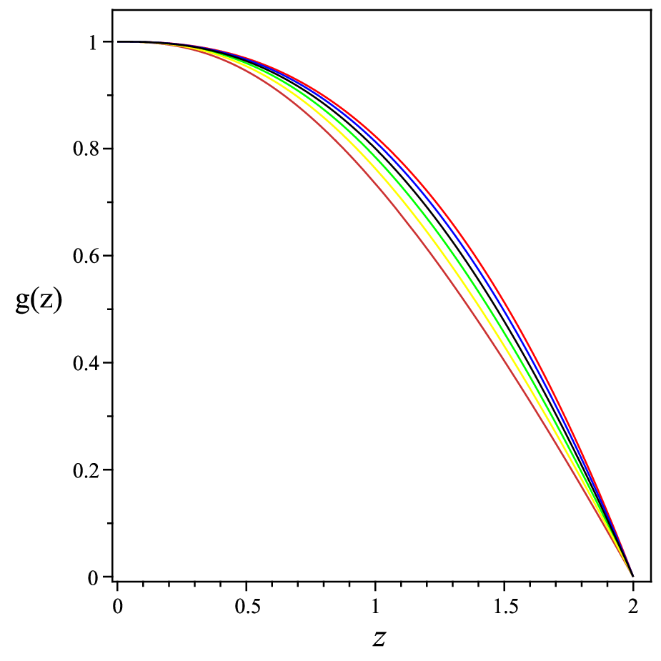
Figure 1: Plot of g⁡(z)g(z) in terms of zz for α=0,0.5,1,1.5,2\alpha={\color[rgb]{1,0,0}0},{\color[rgb]{0,0,1}0.5},1,{\color[rgb]{0,1,0}1.5},{\color[rgb]{1,0.5,0}2} (left), ν=1,2,3,4,5,6\nu={\color[rgb]{1,0,0}1},{\color[rgb]{0,0,1}2},3,{\color[rgb]{0,1,0}4},{\color[rgb]{1,0.5,0}5},6 (middle) and zh=1,2,3,4,5,6z_{h}={\color[rgb]{1,0,0}1},{\color[rgb]{0,0,1}2},3,{\color[rgb]{0,1,0}4},{\color[rgb]{1,0.5,0}5},6 (right).

The behavior of the metric function is depicted in Fig.(1). The main feature is that the metric function values decrease faster for larger α\alpha (Fig.1a). In the isotropic case (ν=1\nu=1) the metric function values are larger than in the anisotropic ones (ν≠1\nu\neq 1) (Fig.1b). In this panel by increasing ν\nu the metric function values decrease faster. Changing the values of α\alpha and ν\nu does not influence the horizon position. In the following we look at the behavior of Ricci and Kretschmann scalar K=Ra​b​c​d​Ra​b​c​dK=R_{abcd}R^{abcd} of the black brane. The Ricci scalar is given as follows

R\displaystyle R =12​α​ν2​l2​((ν2​l2−4​α)2​zh2​ν+2ν+8​α​(ν2​l2−2​α)​z2​ν+2ν)32[−l2ν2(4ν+3(ν2+1))\displaystyle=\dfrac{1}{2\alpha\nu^{2}l^{2}\left((\nu^{2}l^{2}-4\alpha)^{2}z_{h}^{\frac{2\nu+2}{\nu}}+8\alpha(\nu^{2}l^{2}-2\alpha)z^{\frac{2\nu+2}{\nu}}\right)^{\frac{3}{2}}}[-l^{2}\nu^{2}(4\nu+3(\nu^{2}+1))
((ν2​l2−4​α)2​zh2​ν+2ν+8​α​(ν2​l2−2​α)​z2​ν+2ν)32​(3​(ν2+1)+4​ν)​(ν2​l2−4​α)4​zh3​ν+3ν\displaystyle\left((\nu^{2}l^{2}-4\alpha)^{2}z_{h}^{\frac{2\nu+2}{\nu}}+8\alpha(\nu^{2}l^{2}-2\alpha)z^{\frac{2\nu+2}{\nu}}\right)^{\frac{3}{2}}(3(\nu^{2}+1)+4\nu)(\nu^{2}l^{2}-4\alpha)^{4}z_{h}^{\frac{3\nu+3}{\nu}}
+4​(ν2​l2−2​α)​((ν2​l2−4​α)2​(9​ν2+11​ν+10)​(zh​z2)ν+1ν+8​α​(ν2​l2−2​α)​(2​ν2CLOSECLOSE\displaystyle+4(\nu^{2}l^{2}-2\alpha)((\nu^{2}l^{2}-4\alpha)^{2}(9\nu^{2}+11\nu+10)(z_{h}z^{2})^{\frac{\nu+1}{\nu}}+8\alpha(\nu^{2}l^{2}-2\alpha)(2\nu^{2}
+ν+3)zh−ν−1νz4​ν+4ν)].\displaystyle+\nu+3)z_{h}^{\frac{-\nu-1}{\nu}}z^{\frac{4\nu+4}{\nu}})]. (18)

The scalars are smooth inside the black hole and start to diverge for z>zhz>z_{h}. In larger α\alpha it happens earlier for RR, while for KK it happens earlier for smaller α\alpha.

Refer to caption
(a) ν=4.5,l=1,zh=2\nu=4.5,l=1,z_{h}=2
Refer to caption
(b) ν=4.5,l=1,zh=2\nu=4.5,l=1,z_{h}=2
Figure 2: Plot of Ricci scalar and Kretschmann scalar in terms of zz for α=0.1,0.2,0.3,0.4,0.5\alpha={\color[rgb]{1,0,0}0.1},{\color[rgb]{0,0,1}0.2},0.3,{\color[rgb]{0,1,0}0.4},{\color[rgb]{1,0.5,0}0.5}.

By inserting (2.1) in Et​tE_{tt}, one can obtain ϕ\phi as follows:

ϕ⁡(z)=−2​−2​𝒦​(ν−1)​(ℋ​𝒟​arctan⁡(𝒢ℱ)−ℒ​ℱ​arctan⁡(𝒢𝒟)−2​𝒟​ℱ​𝒢​(l4​ν4−8​α​c2))(ν+1)​l​𝒢​ℱ​ℰ​ν​l4​ν4−8​α​c2​l2​ν3+l2​ν2−ℰ+c3,\displaystyle\phi(z)=\dfrac{-2\sqrt{-2\mathcal{K}(\nu-1)}\left(\sqrt{\mathcal{H}\sqrt{\mathcal{D}}}\arctan\left(\sqrt{\frac{\mathcal{G}}{\mathcal{F}}}\right)-\mathcal{L}\sqrt{\mathcal{F}}\arctan\left(\sqrt{\frac{\mathcal{G}}{\mathcal{D}}}\right)-2\sqrt{\mathcal{DFG}(l^{4}\nu^{4}-8\alpha c_{2})}\right)}{(\nu+1)l\sqrt{\mathcal{GFE}\nu}\sqrt{l^{4}\nu^{4}-8\alpha c_{2}}\sqrt{l^{2}\nu^{3}+l^{2}\nu^{2}-\sqrt{\mathcal{E}}}}+c_{3}, (19)

by imposing the condition ϕ⁡(zh)=0\phi(z_{h})=0, one can obtain c3=0c_{3}=0. The constants 𝒦,ℋ,…\mathcal{K},\mathcal{H},... are provided in (Constants). In the case of α≪1\alpha\ll 1, one can get

ϕ⁡(z)\displaystyle\phi(z) =2​ν−1ν​ln⁡(zzh)−4​α​ν−1l2​ν2​(ν+1)​[(ν+1)​ln⁡(zzh)+ν2​(1−(zzh)2​ν+2ν)]+𝒪⁡(α2).\displaystyle=\dfrac{2\sqrt{\nu-1}}{\nu}\ln\left(\dfrac{z}{z_{h}}\right)-\dfrac{4\alpha\sqrt{\nu-1}}{l^{2}\nu^{2}(\nu+1)}\left[(\nu+1)\ln\left(\dfrac{z}{z_{h}}\right)+\dfrac{\nu}{2}\left(1-\left(\dfrac{z}{z_{h}}\right)^{\frac{2\nu+2}{\nu}}\right)\right]+\mathcal{O}(\alpha^{2}). (20)

The first term is the contribution of the Einstien term and the second term is from the Gauss-Bonnet term. In figure (3), the real and imaginary parts of the scalar field in terms of zz for different values of parameters have been shown. As can be seen the imaginary part of scalar field inside and outside the black brane has a non-zero value and is unstable. By increasing ν\nu in 0<z<zh0<z<z_{h}, the real part and imaginary part of the scalar field increase and decrease respectively and for z>zhz>z_{h} vice versa (Fig.(3)a). In panel b, by increasing the coupling of theory in 0<z<zh0<z<z_{h} the real and imaginary parts decrease and increase respectively, and for z>zhz>z_{h} vice versa.

Refer to caption
(a) α=0.1,l=1,zh=2\alpha=0.1,l=1,z_{h}=2
Refer to caption
(b) α=0.1,l=1,ν=4.5\alpha=0.1,l=1,\nu=4.5
Refer to caption
(c) zh=2,α=0.1,l=1z_{h}=2,\alpha=0.1,l=1
Figure 3: Plots of imagenary (solid lines) and real part (dashed lines) of ϕ\phi in terms of zz for ν=2,3,4,5,6\nu={\color[rgb]{1,0,0}2},{\color[rgb]{0,0,1}3},4,{\color[rgb]{0,1,0}5},{\color[rgb]{1,0.5,0}6} (left), for α=0.1,0.2,0.3,0.4,0.5\alpha={\color[rgb]{1,0,0}0.1},{\color[rgb]{0,0,1}0.2},0.3,{\color[rgb]{0,1,0}0.4},{\color[rgb]{1,0.5,0}0.5} (middle), for zh=2,3,4,5,6z_{h}={\color[rgb]{1,0,0}2},{\color[rgb]{0,0,1}3},4,{\color[rgb]{0,1,0}5},{\color[rgb]{1,0.5,0}6} (right).

By inserting (20) into Ex​xE_{xx}, one can obtain f2f_{2} as follows:

f2\displaystyle f_{2} =−2ν3​q2​α​(ν+1)​𝒜¯52​(ν2​l2​(ν+1)−𝒜¯)[−6ν(ν−1)(ν+1)5αc1𝒞¯(ν4l4−8αc2)(νl2(ν−12)\displaystyle=-\dfrac{2}{\nu^{3}q^{2}\alpha(\nu+1)\bar{\mathcal{A}}^{\frac{5}{2}}(\nu^{2}l^{2}(\nu+1)-\sqrt{\bar{\mathcal{A}}})}[-6\nu(\nu-1)(\nu+1)^{5}\alpha c_{1}\bar{\mathcal{C}}(\nu^{4}l^{4}-8\alpha c_{2})(\nu l^{2}(\nu-\frac{1}{2})
OPEN𝒜¯−𝒦¯)​z2​ν−2ν−8​α3​c13​𝒞¯​ν2​(2​ν2−5​ν−2+ν3)​(ν+1)3​z2+6​νν+2​z4​ν​(ν+1)4​α2​c12​𝒞¯​(ν2​l2​𝒜¯CLOSE\displaystyle\sqrt{\bar{\mathcal{A}}}-\bar{\mathcal{K}})z^{\frac{2\nu-2}{\nu}}-8\alpha^{3}c_{1}^{3}\bar{\mathcal{C}}\nu^{2}(2\nu^{2}-5\nu-2+\nu^{3})(\nu+1)^{3}z^{\frac{2+6\nu}{\nu}}+2z^{4}\nu(\nu+1)^{4}\alpha^{2}c_{1}^{2}\bar{\mathcal{C}}(\nu^{2}l^{2}\sqrt{\bar{\mathcal{A}}}
(2ν2+5−5ν)−ℱ¯)+z−4ν[12(ν2l2(ν+1)2ℰ¯𝒜¯32)+12(ν2l2(ν2−1)ℬ¯𝒜¯52)+νl2(ν−1)(ν+1)6\displaystyle(2\nu^{2}+5-5\nu)-\bar{\mathcal{F}})+z^{-\frac{4}{\nu}}[\frac{1}{2}(\nu^{2}l^{2}(\nu+1)^{2}\bar{\mathcal{E}}\bar{\mathcal{A}}^{\frac{3}{2}})+\frac{1}{2}(\nu^{2}l^{2}(\nu^{2}-1)\bar{\mathcal{B}}\bar{\mathcal{A}}^{\frac{5}{2}})+\nu l^{2}(\nu-1)(\nu+1)^{6}
(ν−12)​𝒞¯​𝒜¯​(ν4​l4−8​α​c2)2−ν15​l8​𝒞¯​𝒢¯−5​ν14​l8​𝒞¯​𝒢¯−9​ν13​l8​𝒞¯​𝒢¯−5​ν12​l8​𝒞¯​𝒢¯+5​ν11​l4​𝒞¯​𝒢¯​(l4+CLOSE\displaystyle(\nu-\frac{1}{2})\bar{\mathcal{C}}\sqrt{\bar{\mathcal{A}}}(\nu^{4}l^{4}-8\alpha c_{2})^{2}-\nu^{15}l^{8}\bar{\mathcal{C}}\bar{\mathcal{G}}-5\nu^{14}l^{8}\bar{\mathcal{C}}\bar{\mathcal{G}}-9\nu^{13}l^{8}\bar{\mathcal{C}}\bar{\mathcal{G}}-5\nu^{12}l^{8}\bar{\mathcal{C}}\bar{\mathcal{G}}+5\nu^{11}l^{4}\bar{\mathcal{C}}\bar{\mathcal{G}}(l^{4}+
OPEN165​α​c2)+9​ν10​l4​𝒞¯​𝒢¯​(l4+809​α​c2)+5​ν9​l4​𝒞¯​𝒢¯​(l4+1445​α​c2)+l4​ν8​𝒞¯​𝒢¯​(l4+80​α​c2)−80​α​ν7​c2​𝒞¯​𝒢¯\displaystyle\frac{16}{5}\alpha c_{2})+9\nu^{10}l^{4}\bar{\mathcal{C}}\bar{\mathcal{G}}(l^{4}+\frac{80}{9}\alpha c_{2})+5\nu^{9}l^{4}\bar{\mathcal{C}}\bar{\mathcal{G}}(l^{4}+\frac{144}{5}\alpha c_{2})+l^{4}\nu^{8}\bar{\mathcal{C}}\bar{\mathcal{G}}(l^{4}+80\alpha c_{2})-80\alpha\nu^{7}c_{2}\bar{\mathcal{C}}\bar{\mathcal{G}}
(l4+45​α​c2)−144​α​c2​ν6​𝒞¯​𝒢¯​(l4+209​α​c2)−80​α​ν5​c2​𝒞¯​𝒢¯​(l4+365​α​c2)−16​α​ν4​c2​𝒞¯​𝒢¯​(l4+20​α​c2)\displaystyle(l^{4}+\frac{4}{5}\alpha c_{2})-144\alpha c_{2}\nu^{6}\bar{\mathcal{C}}\bar{\mathcal{G}}(l^{4}+\frac{20}{9}\alpha c_{2})-80\alpha\nu^{5}c_{2}\bar{\mathcal{C}}\bar{\mathcal{G}}(l^{4}+\frac{36}{5}\alpha c_{2})-16\alpha\nu^{4}c_{2}\bar{\mathcal{C}}\bar{\mathcal{G}}(l^{4}+20\alpha c_{2})
+320α2ν3c22𝒞¯𝒢¯+ν2ℒ¯+ν𝒥¯+12ℬ¯𝒜¯3+64α2c22𝒞¯𝒢¯]],\displaystyle+320\alpha^{2}\nu^{3}c_{2}^{2}\bar{\mathcal{C}}\bar{\mathcal{G}}+\nu^{2}\bar{\mathcal{L}}+\nu\bar{\mathcal{J}}+\frac{1}{2}\bar{\mathcal{B}}\bar{\mathcal{A}}^{3}+64\alpha^{2}c_{2}^{2}\bar{\mathcal{C}}\bar{\mathcal{G}}]], (21)

where the constants 𝒜¯\bar{\mathcal{A}}, ℬ¯\bar{\mathcal{B}}… are provided in (Constants). In the case of α≪1\alpha\ll 1, one can get

f2\displaystyle f_{2} =4​l2​(ν2−1)​z−4νν2​q2−8​(ν2−1)​z4​αq2​ν4​(z2​ν+2ν−zh2​ν+2ν)2×\displaystyle=\dfrac{4l^{2}(\nu^{2}-1)z^{-\frac{4}{\nu}}}{\nu^{2}q^{2}}-\dfrac{8(\nu^{2}-1)z^{4}\alpha}{q^{2}\nu^{4}\left(z^{\frac{2\nu+2}{\nu}}-z_{h}^{\frac{2\nu+2}{\nu}}\right)^{2}}\times
[−4​ν​(zhz)2​ν+2ν+3​(zzh)4​ν+4ν−6​(zzh)2​ν+2ν+ν​(zhz)4​ν+4ν+(2​ν+3)]+𝒪⁡(α2).\displaystyle\left[-4\nu\left(\dfrac{z_{h}}{z}\right)^{\frac{2\nu+2}{\nu}}+3\left(\dfrac{z}{z_{h}}\right)^{\frac{4\nu+4}{\nu}}-6\left(\dfrac{z}{z_{h}}\right)^{\frac{2\nu+2}{\nu}}+\nu\left(\dfrac{z_{h}}{z}\right)^{\frac{4\nu+4}{\nu}}+(2\nu+3)\right]+\mathcal{O}(\alpha^{2}). (22)

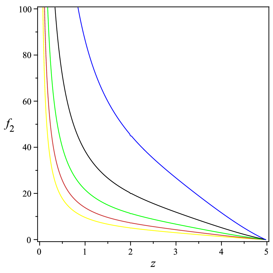
The first terms is the contribution of Einstien gravity and the second term is related to the Gauss-Bonnet gravity. In figure (4), the behavior of f2f_{2} in terms of zz are shown. As can be seen, by increasing α\alpha and qq, f2f_{2} decreases and by increasing ν\nu, f2f_{2} increases.

Refer to caption
(a) ν=4.5,l=1,zh=2,q=0.5\nu=4.5,l=1,z_{h}=2,q=0.5
Refer to caption
(b) ν=4.5,l=1,zh=2,α=0.1\nu=4.5,l=1,z_{h}=2,\alpha=0.1
Refer to caption
(c) l=1,α=0.1,q=0.5,zh=2l=1,\alpha=0.1,q=0.5,z_{h}=2
Figure 4: Plots of f2f_{2} in terms of zz for α=0.1,0.2,0.3,0.4,0.5\alpha={\color[rgb]{1,0,0}0.1},{\color[rgb]{0,0,1}0.2},0.3,{\color[rgb]{0,1,0}0.4},{\color[rgb]{1,0.5,0}0.5} (left), q=0.1,0.2,0.3,0.4,0.5q={\color[rgb]{1,0,0}0.1},{\color[rgb]{0,0,1}0.2},0.3,{\color[rgb]{0,1,0}0.4},{\color[rgb]{1,0.5,0}0.5} (middle), ν=1,2,3,4,5\nu={\color[rgb]{1,0,0}1},{\color[rgb]{0,0,1}2},3,{\color[rgb]{0,1,0}4},{\color[rgb]{1,0.5,0}5} (right).

Finally from Et​tE_{tt}, one can get V⁡(z)V(z) (We did not bring it here due to its bulk). In the case of α≪1\alpha\ll 1, one can get

V⁡(z)\displaystyle V(z) =−2​(ν+1)​(2​ν+1)ν2​l2+α(z2​ν+2ν−zh2​ν+2ν)3​ν4​l4[−4z4​ν+4νzh2​ν+2ν(−1−7ν+6ν3+20ν2)\displaystyle=-\dfrac{2(\nu+1)(2\nu+1)}{\nu^{2}l^{2}}+\dfrac{\alpha}{\left(z^{\frac{2\nu+2}{\nu}}-z_{h}^{\frac{2\nu+2}{\nu}}\right)^{3}\nu^{4}l^{4}}[-4z^{\frac{4\nu+4}{\nu}}z_{h}^{\frac{2\nu+2}{\nu}}(-1-7\nu+6\nu^{3}+20\nu^{2})
+8​ν​(3​ν2+7​ν−1)​z2​ν+2ν​zh4​ν+4ν+(8​ν3+64​ν2−36​ν−12)​z6​ν+6ν+4​(ν−1)​(2​ν+1)​z10​ν+10ν​zh−4​ν−4ν\displaystyle+8\nu(3\nu^{2}+7\nu-1)z^{\frac{2\nu+2}{\nu}}z_{h}^{\frac{4\nu+4}{\nu}}+(8\nu^{3}+64\nu^{2}-36\nu-12)z^{\frac{6\nu+6}{\nu}}+4(\nu-1)(2\nu+1)z^{\frac{10\nu+10}{\nu}}z_{h}^{\frac{-4\nu-4}{\nu}}
−4(ν−1)(8ν+3)z8​ν+8νzh−2​ν−2ν−8ν2(ν+2)zh6​ν+6ν]+𝒪(α2).\displaystyle-4(\nu-1)(8\nu+3)z^{\frac{8\nu+8}{\nu}}z_{h}^{\frac{-2\nu-2}{\nu}}-8\nu^{2}(\nu+2)z_{h}^{\frac{6\nu+6}{\nu}}]+\mathcal{O}(\alpha^{2}). (23)

In Fig. (5), the behavior of scalar potential in terms of zz for anisotropic case has been shown. In the left panel, between 0<z<zh0<z<z_{h} by increasing α\alpha, the potential decreases. In the right panel, between 0<z<zh0<z<z_{h} by increasing ν\nu the scalar potential increases.

Refer to caption
(a) ν=4.5,zh=2,l=1\nu=4.5,z_{h}=2,l=1
Refer to caption
(b) ν=4.5,l=1,zh=2\nu=4.5,l=1,z_{h}=2
Figure 5: Plots of VV in terms of zz for α=0.1,0.2,0.3,0.4,0.5\alpha={\color[rgb]{1,0,0}0.1},{\color[rgb]{0,0,1}0.2},0.3,{\color[rgb]{0,1,0}0.4},{\color[rgb]{1,0.5,0}0.5} (left), ν=1,2,3,4,5\nu={\color[rgb]{1,0,0}1},{\color[rgb]{0,0,1}2},3,{\color[rgb]{0,1,0}4},{\color[rgb]{1,0.5,0}5} (right).

2.1.1 Thermodynamics of the background

In this subsection, we explore the thermodynamics of the black brane solution (2.1). In order to investigate the thermodynamic properties of the black brane we need to obtain some relevant thermodynamic quantities. The temperature of the black brane is obtained as follows:

T=|g′4​π|=ν+12​π​zh​ν​(1−2​αν2​l2).\displaystyle T=\left|\dfrac{g^{\prime}}{4\pi}\right|=\dfrac{\nu+1}{2\pi z_{h}\nu}\left(1-\dfrac{2\alpha}{\nu^{2}l^{2}}\right). (24)

It is noticed that, the temperature monotonically decreases with the increase of the horizon. By increasing α\alpha, the temperature is decreased, and for α=0\alpha=0, one can get the result of [8]. The entropy is given as follows [32],[33]

S=−18∫Σdn−2xηδ​Lδ​Rμ​α​β​νϵμ​αϵβ​ν,\displaystyle S=-\dfrac{1}{8}\int_{\Sigma}d^{n-2}x\sqrt{\eta}\dfrac{\delta L}{\delta R_{\mu\alpha\beta\nu}}\epsilon_{\mu\alpha}\epsilon_{\beta\nu}, (25)

where

δ​Lδ​Rμ​α​β​ν=\displaystyle\dfrac{\delta L}{\delta R_{\mu\alpha\beta\nu}}= (12+α​R)​(gμ​β​gα​ν−gμ​ν​gα​β)+12​β​(Rμ​β​gα​ν−Rα​β​gμ​ν−Rμ​ν​gα​β+Rα​ν​gμ​β)\displaystyle\left(\dfrac{1}{2}+\alpha R\right)\left(g^{\mu\beta}g^{\alpha\nu}-g^{\mu\nu}g^{\alpha\beta}\right)+\dfrac{1}{2}\beta\left(R^{\mu\beta}g^{\alpha\nu}-R^{\alpha\beta}g^{\mu\nu}-R^{\mu\nu}g^{\alpha\beta}+R^{\alpha\nu}g^{\mu\beta}\right)
+2​γ​Rμ​α​β​ν,\displaystyle+2\gamma R^{\mu\alpha\beta\nu}, (26)

and ϵμ​ν=−2−hδt[μδzν]\epsilon_{\mu\nu}=-2\sqrt{-h}\delta^{t}_{[\mu}\delta^{z}_{\nu]}. For c=0c=0 we have

s=S𝒱=l3​P​(zh)​b​(zh)324​zh3=l34​zhν+2ν,s=\dfrac{S}{\mathcal{V}}=\dfrac{l^{3}P(z_{h})b(z_{h})^{\frac{3}{2}}}{4z_{h}^{3}}=\dfrac{l^{3}}{4z_{h}^{\frac{\nu+2}{\nu}}}, (27)

which is independent of parameter of the EGB gravity. In terms of the temperature, the entropy is given as

s=l34​(2​π​T​ν3​l2(ν+1)​(ν2​l2−2​α))ν+2ν.s=\dfrac{l^{3}}{4}\left(\dfrac{2\pi T\nu^{3}l^{2}}{(\nu+1)(\nu^{2}l^{2}-2\alpha)}\right)^{\frac{\nu+2}{\nu}}. (28)

For isotropic case s≈T3s\approx T^{3} and for anisotropic case s≈Tν+1νs\approx T^{\frac{\nu+1}{\nu}}. The free energy density F⁡(T)F(T) can be calculated from the entropy density s⁡(T)s(T) by integrating as follows

F=∫s​𝑑T=ν2​(ν+1)​T​s,F=\int sdT=\dfrac{\nu}{2(\nu+1)}Ts, (29)

which is related to temperature as F≈T2​ν+1νF\approx T^{\frac{2\nu+1}{\nu}}. The sound velocity cs2c_{s}^{2} which can directly measure the conformality of the system, can be obtained from the temperature and entropy:

cs2=d​log⁡Td​log⁡s=νν+2.c_{s}^{2}=\dfrac{d\log T}{d\log s}=\dfrac{\nu}{\nu+2}. (30)

For isotropic case (ν=1\nu=1), cs2=1/3c_{s}^{2}=1/3, the system is conformal, for anisotropic (ν≠1\nu\neq 1), cs2≠1/3c_{s}^{2}\neq 1/3 the system is non-conformal. The heat capacity is given as

CV=T​d​sd​T=(ν+2)ν​s=scs2.C_{V}=T\dfrac{ds}{dT}=\dfrac{(\nu+2)}{\nu}s=\dfrac{s}{c_{s}^{2}}. (31)

In terms of temperature,

CVT3=l3​(ν+2)4​ν​(2​π​ν3​l2(ν+1)​(ν2​l2−2​α))ν+2ν​T2−2​νν.\dfrac{C_{V}}{T^{3}}=\dfrac{l^{3}(\nu+2)}{4\nu}\left(\dfrac{2\pi\nu^{3}l^{2}}{(\nu+1)(\nu^{2}l^{2}-2\alpha)}\right)^{\frac{\nu+2}{\nu}}T^{\frac{2-2\nu}{\nu}}. (32)

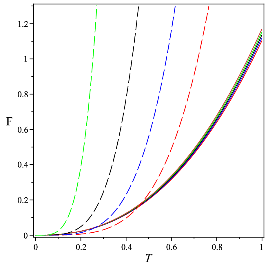
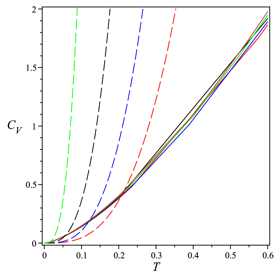
For isotropic case, the right hand side of (32) has a constant value and for ν>1\nu>1 depends to the temperature and at high temperature goes to zero. Since entropy is positive therefore CVC_{V} is positive and the black hole is stable. In figure 6, the behavior of ss, FF and CVC_{V} in terms of TT for isotropic (dashed lines) and anisotropic (solid lines) and different values of α\alpha have been shown. As can be seen, by increasing α\alpha, the thermodynamical quantities ss, FF, and CVC_{V} increase. For T<Tc​r​o​s​siT<T^{i}_{cross}, the entropy, free energy, and heat capacity of anisotropic case is larger than isotropic, and for T>Tc​r​o​s​siT>T^{i}_{cross} vice versa. Where i=s,F,CVi=s,F,C_{V} and Tc​r​o​s​siT^{i}_{cross} are given as follows

Refer to caption
(a) l=1l=1
Refer to caption
(b) l=1l=1
Refer to caption
(c) l=1l=1
Figure 6: Plots of ss, FF and CVC_{V} in terms of TT for α=0.1,0.2,0.3,0.4,0.5\alpha={\color[rgb]{1,0,0}0.1},{\color[rgb]{0,0,1}0.2},0.3,{\color[rgb]{0,1,0}0.4},{\color[rgb]{1,0.5,0}0.5} and ν=4.5\nu=4.5 (solid line) and ν=1\nu=1 (dashed lines) .
Tc​r​o​s​ss=\displaystyle T^{s}_{cross}= [l4​((l2−2​α)3​ν3​(ν+2)ν​π2​(1−ν)ν​2ν+2ν)νl4​ν​((ν+1)​(l2​ν2−2​α))2​(ν+1)​(l2​ν2−2​α)ν]12​ν−2,\displaystyle\left[\dfrac{l^{4}((l^{2}-2\alpha)^{3}\nu^{\frac{3(\nu+2)}{\nu}}\pi^{\frac{2(1-\nu)}{\nu}}2^{\frac{\nu+2}{\nu}})^{\nu}}{l^{4\nu}((\nu+1)(l^{2}\nu^{2}-2\alpha))^{2}(\nu+1)(l^{2}\nu^{2}-2\alpha)^{\nu}}\right]^{\frac{1}{2\nu-2}}, (33)
Tc​r​o​s​sF=\displaystyle T_{cross}^{F}= ((l2−2​α)2​4ν+1ν​π2−2​ννν−3​ν−6ν+ν−4​ν−6ν)ν2​(ν−1)[(ν+1)​(l2​ν2−2​α)ν+2​l4​(ν−1)]12​ν−2,\displaystyle\dfrac{\left(\dfrac{(l^{2}-2\alpha)^{2}4^{\frac{\nu+1}{\nu}}\pi^{\frac{2-2\nu}{\nu}}}{\nu^{\frac{-3\nu-6}{\nu}}+\nu^{\frac{-4\nu-6}{\nu}}}\right)^{\frac{\nu}{2(\nu-1)}}}{[(\nu+1)(l^{2}\nu^{2}-2\alpha)^{\nu+2}l^{4(\nu-1)}]^{\frac{1}{2\nu-2}}}, (34)
Tc​r​o​s​sCV=\displaystyle T^{C_{V}}_{cross}= [l4​(ν+1)​((l2​ν2−2​α)3​(ν+2)​ν2​(ν+1)ν​π2​(1−ν)ν​2ν+2ν)ν3ν​(ν+1)​(l2​ν2−2​α)ν+2]12​ν−2.\displaystyle\left[\dfrac{l^{4(\nu+1)}((l^{2}\nu^{2}-2\alpha)^{3}(\nu+2)\nu^{\frac{2(\nu+1)}{\nu}}\pi^{\frac{2(1-\nu)}{\nu}}2^{\frac{\nu+2}{\nu}})^{\nu}}{3^{\nu}(\nu+1)(l^{2}\nu^{2}-2\alpha)^{\nu+2}}\right]^{\frac{1}{2\nu-2}}. (35)

2.2 The case c≠0,μ=0c\neq 0,\mu=0

In this case At=0A_{t}=0 and the differential equation (2), becomes

4​ν​l​z2​e−c​z24​(l2​ν2​e−c​z22−α​(2+ν​c​z2)2​g​(z))​g′′−2​z​l​e−c​z24​(ν2​l2​(4+(2+3​z2)​ν)−CLOSE\displaystyle 4\nu lz^{2}e^{-\frac{cz^{2}}{4}}(l^{2}\nu^{2}e^{-\frac{cz^{2}}{2}}-\alpha(2+\nu cz^{2})^{2}g(z))g^{\prime\prime}-2zle^{-\frac{cz^{2}}{4}}(\nu^{2}l^{2}(4+(2+3z^{2})\nu)-
OPENα⁡(2+ν​c​z2)​(8+4​ν+6​ν​c​z2−6​c​ν2​z2+c2​ν2​z4)​g)​g′−4​α​ν​z2​l​e−c​z24​(2+ν​c​z2)2​g′2=0.\displaystyle\alpha(2+\nu cz^{2})(8+4\nu+6\nu cz^{2}-6c\nu^{2}z^{2}+c^{2}\nu^{2}z^{4})g)g^{\prime}-4\alpha\nu z^{2}le^{-\frac{cz^{2}}{4}}(2+\nu cz^{2})^{2}g^{\prime 2}=0. (36)

In order to solve equation (2.2), we assume g⁡(z)g(z) as follows

g⁡(z)=1+ϵ​g1​(z)+𝒪⁡(ϵ2),g(z)=1+\epsilon g_{1}(z)+\mathcal{O}(\epsilon^{2}), (37)

by inserting it into the (2.2), one can achieve a homogeneous differential equation for g1​(z)g_{1}(z) as

g1′′+[−l2​ν3​(2+3​c​z2)−4​ν2​(l2+4​α​c​z2)+4​α​ν​(2+c​z2)+16​α]​g1′ν​z​(l2​ν2−4​α)=0.g_{1}^{\prime\prime}+\dfrac{[-l^{2}\nu^{3}(2+3cz^{2})-4\nu^{2}(l^{2}+4\alpha cz^{2})+4\alpha\nu(2+cz^{2})+16\alpha]g_{1}^{\prime}}{\nu z(l^{2}\nu^{2}-4\alpha)}=0. (38)

Solving (38) give g1​(z)g_{1}(z) as

g1​(z)=c1+c2​erf​(12​c⁡(−6​l2​ν2−32​ν​α+8​α)(l2​ν2−4​α)​z),\displaystyle g_{1}(z)=c_{1}+c_{2}\text{erf}\left(\dfrac{1}{2}\sqrt{\dfrac{c(-6l^{2}\nu^{2}-32\nu\alpha+8\alpha)}{(l^{2}\nu^{2}-4\alpha)}}z\right), (39)

where c1c_{1} and c2c_{2} are constants of integration. Using (39), the metric (37) becomes

g⁡(z)=1+c1+c2​erf​(12​c⁡(−6​l2​ν2−32​ν​α+8​α)(l2​ν2−4​α)​z).g(z)=1+c_{1}+c_{2}\text{erf}\left(\dfrac{1}{2}\sqrt{\dfrac{c(-6l^{2}\nu^{2}-32\nu\alpha+8\alpha)}{(l^{2}\nu^{2}-4\alpha)}}z\right). (40)

The conditions (9) give us c1c_{1} and c2c_{2} as

c1=0,c2=−1erf​(12​c⁡(−6​l2​ν2−32​ν​α+8​α)(l2​ν2−4​α)​zh).c_{1}=0,\;\;\;\;c_{2}=-\dfrac{1}{\text{erf}\left(\dfrac{1}{2}\sqrt{\dfrac{c(-6l^{2}\nu^{2}-32\nu\alpha+8\alpha)}{(l^{2}\nu^{2}-4\alpha)}}z_{h}\right)}. (41)

Finally, using (41) the metric function becomes

g⁡(z)=1−erf​(12​c⁡(−6​l2​ν2−32​ν​α+8​α)(l2​ν2−4​α)​z)erf​(12​c⁡(−6​l2​ν2−32​ν​α+8​α)(l2​ν2−4​α)​zh).g(z)=1-\dfrac{\text{erf}\left(\dfrac{1}{2}\sqrt{\dfrac{c(-6l^{2}\nu^{2}-32\nu\alpha+8\alpha)}{(l^{2}\nu^{2}-4\alpha)}}z\right)}{\text{erf}\left(\dfrac{1}{2}\sqrt{\dfrac{c(-6l^{2}\nu^{2}-32\nu\alpha+8\alpha)}{(l^{2}\nu^{2}-4\alpha)}}z_{h}\right)}. (42)

In the case of α≪1\alpha\ll 1 and c<0c<0, the blakening function become

g⁡(z)≈1−erf​(−6​c​z2)erf​(−6​c​zh2)−4​(2​ν+1)​−6​c​α​(z​e3​c​z22​erf​(−6​c​zh2)−zh​erf​(−6​c​z2)​e3​c​zh22)3​π​l2​ν2​erf​(−6​c​zh2)2+𝒪⁡(α2),g(z)\approx 1-\dfrac{\text{erf}\left(\dfrac{\sqrt{-6c}z}{2}\right)}{\text{erf}\left(\dfrac{\sqrt{-6c}z_{h}}{2}\right)}-\dfrac{4(2\nu+1)\sqrt{-6c}\alpha\left(ze^{\frac{3cz^{2}}{2}}\text{erf}\left(\dfrac{\sqrt{-6c}z_{h}}{2}\right)-z_{h}\text{erf}\left(\dfrac{\sqrt{-6c}z}{2}\right)e^{\frac{3cz_{h}^{2}}{2}}\right)}{3\sqrt{\pi}l^{2}\nu^{2}\text{erf}\left(\dfrac{\sqrt{-6c}z_{h}}{2}\right)^{2}}+\mathcal{O}\left(\alpha^{2}\right), (43)

and for α≪1\alpha\ll 1 and c>0c>0, we have

g⁡(z)≈1−zzh​e3​c​(z2−zh2)2−2​α​c​(2​ν+1)ν2​l2​z⁡(z2−zh2)zh​e3​c​(z2−zh2)2+𝒪⁡(α2).g(z)\approx 1-\dfrac{z}{z_{h}}e^{\frac{3c(z^{2}-z_{h}^{2})}{2}}-\dfrac{2\alpha c(2\nu+1)}{\nu^{2}l^{2}}\dfrac{z(z^{2}-z_{h}^{2})}{z_{h}}e^{\frac{3c(z^{2}-z_{h}^{2})}{2}}+\mathcal{O}(\alpha^{2}). (44)

In figure (7), the behavior of g⁡(z)g(z) for positive and negative values of warp function is depicted. As cc increases, the metric slope becomes more decreasing. Also, changing the value of cc has no effect on the value of the horizon. By substituting the obtained metric (42), we arrive at the differential equation for the scalar field as:

Refer to caption
(a) ν=4.5,α=0.1,l=1,zh=2\nu=4.5,\alpha=0.1,l=1,z_{h}=2
Refer to caption
(b) α=0.1,l=1,zh=2\alpha=0.1,l=1,z_{h}=2
Figure 7: Plots of g⁡(z)g(z) in terms of zz for c=0.5,0.4,0.3,0.2,0.1c={\color[rgb]{1,0,0}0.5},{\color[rgb]{0,0,1}0.4},0.3,{\color[rgb]{0,1,1}0.2},{\color[rgb]{1,0.5,0}0.1} (dashed lines) and −0.5,−0.4,−0.3,−0.2,−0.1{\color[rgb]{1,0,0}-0.5},{\color[rgb]{0,0,1}-0.4},-0.3,{\color[rgb]{0,1,0}-0.2},{\color[rgb]{1,0.5,0}-0.1} (solid lines) (left), ν=1,2,3,4,5,6\nu=1,2,3,4,5,6, c=0.5{\color[rgb]{1,0,0}c=0.5} and c=−0.5{\color[rgb]{0,0,1}c=-0.5} (right).
ϕ′2\displaystyle\phi^{\prime 2} =ec​z22z2​l2​ν3​2​π​(l2​ν2−4​α)​erf​(−2​c​𝔸​zh2)​[erf​(−2​c​𝔸​zh2)−erf​(−2​c​𝔸​z2)][2α−2​c​π​𝔸z(2+νcz2)\displaystyle=\dfrac{e^{\frac{cz^{2}}{2}}}{z^{2}l^{2}\nu^{3}{2\pi(l^{2}\nu^{2}-4\alpha)\text{erf}\left(\frac{\sqrt{-2c\mathbb{A}}z_{h}}{2}\right)\left[\text{erf}\left(\frac{\sqrt{-2c\mathbb{A}}z_{h}}{2}\right)-\text{erf}\left(\frac{\sqrt{-2c\mathbb{A}}z}{2}\right)\right]}}[2\alpha\sqrt{-2c\pi\mathbb{A}}z(2+\nu cz^{2})
[−erf​(−2​c​𝔸​zh2)+erf​(−2​c​𝔸​z2)]​e𝔸​c​z22​(ν2​c2​z4​(5​l2​ν2+32​α​ν−4​α)−4​(ν+2)​(l2​ν2−4​α)CLOSE\displaystyle\left[-\text{erf}\left(\frac{\sqrt{-2c\mathbb{A}}z_{h}}{2}\right)+\text{erf}\left(\frac{\sqrt{-2c\mathbb{A}}z}{2}\right)\right]e^{\frac{\mathbb{A}cz^{2}}{2}}(\nu^{2}c^{2}z^{4}(5l^{2}\nu^{2}+32\alpha\nu-4\alpha)-4(\nu+2)(l^{2}\nu^{2}-4\alpha)
OPEN+2​ν​c​z2​(3​ν3​l2+20​α​ν+3​l2​ν2+4​α))−8​c​α​ν​z2​(2+ν​c​z2)2​(3​l2​ν2+16​α​ν−4​α)​e𝔸​c​z2\displaystyle+2\nu cz^{2}(3\nu^{3}l^{2}+20\alpha\nu+3l^{2}\nu^{2}+4\alpha))-8c\alpha\nu z^{2}(2+\nu cz^{2})^{2}(3l^{2}\nu^{2}+16\alpha\nu-4\alpha)e^{\mathbb{A}cz^{2}}
+2​l2​ν2​z​−2​c​π​𝔸​erf​(−2​c​𝔸​zh2)​ec​z2​ν​(ν​l2+8​α)ν2​l2−4​α​(ν​c​z2​(3​l2​ν2+32​α​ν+4​α)−2​(ν+2)​(l2​ν2−4​α))\displaystyle+2l^{2}\nu^{2}z\sqrt{-2c\pi\mathbb{A}}\text{erf}\left(\frac{\sqrt{-2c\mathbb{A}}z_{h}}{2}\right)e^{\frac{cz^{2}\nu(\nu l^{2}+8\alpha)}{\nu^{2}l^{2}-4\alpha}}(\nu cz^{2}(3l^{2}\nu^{2}+32\alpha\nu+4\alpha)-2(\nu+2)(l^{2}\nu^{2}-4\alpha))
−π⁡(l2​ν2−4​α)​(erf​(−2​c​𝔸​z2)−erf​(−2​c​𝔸​zh2))​(l2​ν​e−c​z22​erf​(−2​c​𝔸​zh2)​(−8+8​ν+3​ν2​c2​z4CLOSECLOSE\displaystyle-\pi(l^{2}\nu^{2}-4\alpha)\left(\text{erf}(\frac{\sqrt{-2c\mathbb{A}}z}{2})-\text{erf}(\frac{\sqrt{-2c\mathbb{A}}z_{h}}{2})\right)(l^{2}\nu e^{-\frac{cz^{2}}{2}}\text{erf}(\frac{\sqrt{-2c\mathbb{A}z_{h}}}{2})(-8+8\nu+3\nu^{2}c^{2}z^{4}
OPEN+18​ν2​c​z2)+α⁡(2+ν​c​z2)​(erf​(−2​c​𝔸​z2)−erf​(−2​c​𝔸​zh2))​(−16+16​ν+3​ν2​z6​c3+2​ν​c2​z4​(1+CLOSECLOSE\displaystyle+18\nu^{2}cz^{2})+\alpha(2+\nu cz^{2})(\text{erf}(\frac{\sqrt{-2c\mathbb{A}}z}{2})-\text{erf}(\frac{\sqrt{-2c\mathbb{A}}z_{h}}{2}))(-16+16\nu+3\nu^{2}z^{6}c^{3}+2\nu c^{2}z^{4}(1+
11ν)+4cz2(6ν2−2+5ν)))]\displaystyle 11\nu)+4cz^{2}(6\nu^{2}-2+5\nu)))] (45)

where

𝔸=3​l2​ν2+16​ν​α−4​αl2​ν2−4​α.\mathbb{A}=\dfrac{3l^{2}\nu^{2}+16\nu\alpha-4\alpha}{l^{2}\nu^{2}-4\alpha}. (46)

In figure 8, the behavior of imaginary and real part of ϕ⁡(z)\phi(z) in terms of zz for different values of parameters has been shown. As can be seen, the imaginary part of scalar field inside the black hole is zero and outside the black hole the scalar field is unstable, and by increasing α\alpha instability increase.

Refer to caption
(a) ν=4.5,α=0.1,l=1,zh=2\nu=4.5,\alpha=0.1,l=1,z_{h}=2
Refer to caption
(b) ν=4.5,l=1,zh=2,c=−0.5\nu=4.5,l=1,z_{h}=2,c=-0.5
Figure 8: Plots of real (dashed lines) and imagenary (solid lines) part of ϕ\phi in terms of zz for c=−0.1,−0.2,−0.3,−0.4,−0.5c={\color[rgb]{1,0,0}-0.1},{\color[rgb]{0,0,1}-0.2},-0.3,{\color[rgb]{0,1,0}-0.4},{\color[rgb]{1,1,0}-0.5} (left), α=0.1,0.2,0.3,0.4\alpha={\color[rgb]{0,0,1}0.1},0.2,{\color[rgb]{0,1,0}0.3},{\color[rgb]{1,1,0}0.4},0.5 (right).

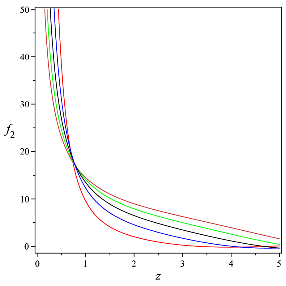
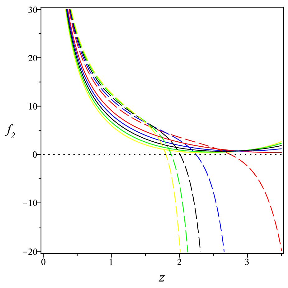
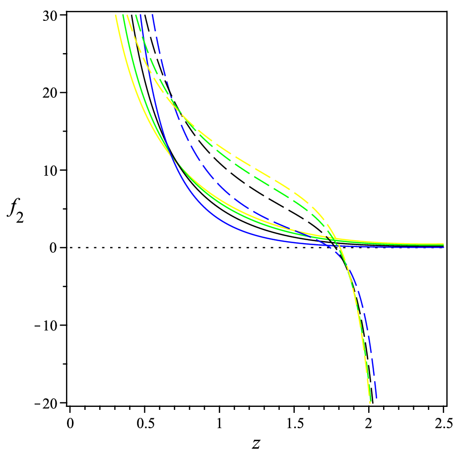
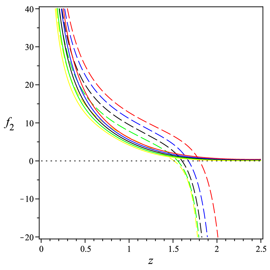
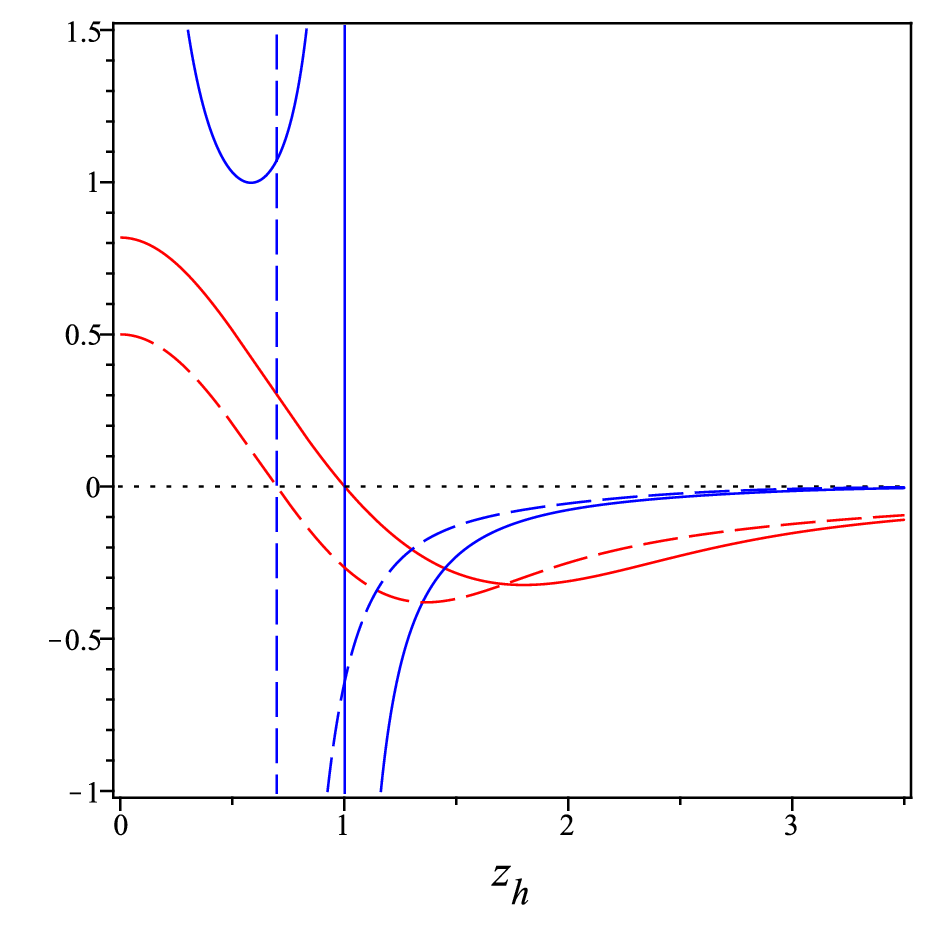
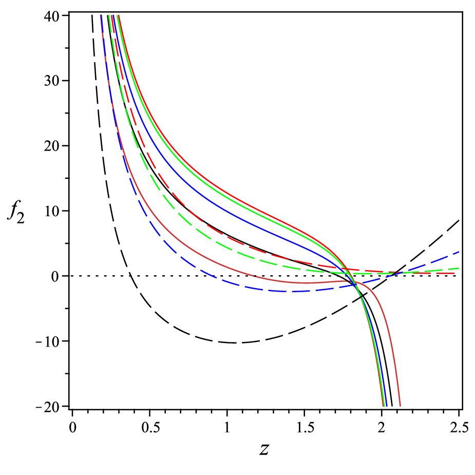
In equation (2.2) the exact coupling function f2f_{2} and approximatly to first order in α\alpha in equation (2.2) has been obtained. In figure (9), f2f_{2} for positive/negative cc and for different values of parameters has been plotted. The important feature of the figures is that for the negative cc, f2f_{2} goes to the negative values by increasing zz, while it does not become negative anywhere for the positive cc.

f2\displaystyle f_{2} =(1−ν)​z−4νπ32​ν3​q2​(l2​ν2−4​α)​erf​(−2​c​𝔸​zh2)2[πzα𝔸ec​𝔸​z22[erf(−2​c​𝔸​z2)−erf(−2​c​𝔸​zh2)](cz2l2ν4(cz2−6)\displaystyle=\dfrac{(1-\nu)z^{-\frac{4}{\nu}}}{\pi^{\frac{3}{2}}\nu^{3}q^{2}(l^{2}\nu^{2}-4\alpha)\text{erf}\left(\frac{\sqrt{-2c\mathbb{A}}z_{h}}{2}\right)^{2}}[\pi z\alpha\sqrt{\mathbb{A}}e^{\frac{c\mathbb{A}z^{2}}{2}}\left[\text{erf}\left(\frac{\sqrt{-2c\mathbb{A}}z}{2}\right)-\text{erf}\left(\frac{\sqrt{-2c\mathbb{A}}z_{h}}{2}\right)\right](cz^{2}l^{2}\nu^{4}(cz^{2}-6)
OPEN+ν3​(32​c2​z4​α−2​l2​(c​z2+10))+ν2​(−8​l2+α⁡(12​c2​z4+88​c​z2))+40​α​ν​(c​z2+2)+32​α)−4​π​α​c​z2​ν​(2+CLOSE\displaystyle+\nu^{3}(32c^{2}z^{4}\alpha-2l^{2}(cz^{2}+10))+\nu^{2}(-8l^{2}+\alpha(12c^{2}z^{4}+88cz^{2}))+40\alpha\nu(cz^{2}+2)+32\alpha)-4\sqrt{\pi}\alpha cz^{2}\nu(2+
OPENν​c​z2)​(3​l2​ν2+16​α​ν−4​α)​ec​𝔸​z2+(l2​ν2−4​α)​(−2​l2​ν2​π​z​−2​c​𝔸​ec​z2​ν​(l2​ν+8​α)l2​ν2−4​α​erf​(−2​c​𝔸​zh2)+π32CLOSE\displaystyle\nu cz^{2})(3l^{2}\nu^{2}+16\alpha\nu-4\alpha)e^{c\mathbb{A}z^{2}}+(l^{2}\nu^{2}-4\alpha)(-2l^{2}\nu^{2}\pi z\sqrt{-2c\mathbb{A}}e^{\frac{cz^{2}\nu(l^{2}\nu+8\alpha)}{l^{2}\nu^{2}-4\alpha}}\text{erf}\left(\frac{\sqrt{-2c\mathbb{A}}z_{h}}{2}\right)+\pi^{\frac{3}{2}}
[erf(−2​c​𝔸​z2)−erf(−2​c​𝔸​zh2)](l2νerf(−2​c​𝔸​zh2)e−c​z22(3νcz2+4ν+4)+[erf(−2​c​𝔸​z2)−\displaystyle\left[\text{erf}\left(\frac{\sqrt{-2c\mathbb{A}}z}{2}\right)-\text{erf}\left(\frac{\sqrt{-2c\mathbb{A}}z_{h}}{2}\right)\right](l^{2}\nu\text{erf}\left(\frac{\sqrt{-2c\mathbb{A}}z_{h}}{2}\right)e^{-\frac{cz^{2}}{2}}(3\nu cz^{2}+4\nu+4)+[\text{erf}\left(\frac{\sqrt{-2c\mathbb{A}}z}{2}\right)-
erf(−2​c​𝔸​zh2)]α(16+8cz2+ν2(z6c3−2c2z4)+ν(16+6c2z4+12cz2))],\displaystyle\text{erf}\left(\frac{\sqrt{-2c\mathbb{A}}z_{h}}{2}\right)]\alpha(16+8cz^{2}+\nu^{2}(z^{6}c^{3}-2c^{2}z^{4})+\nu(16+6c^{2}z^{4}+12cz^{2}))], (47)

In the case of α≪1\alpha\ll 1 and c<0c<0 one can get

f2≈l2​(ν−1)​e−c​z22​[2​−6​c​z​ν​e3​c​z22−π12​(4+4​ν+3​ν​c​z2)​(erf​(−6​c​z2)−erf​(−6​c​zh2))]ν2​q2​z4ν​q2​π12​erf​(−6​c​zh2)\displaystyle f_{2}\approx\dfrac{l^{2}(\nu-1)e^{-\frac{cz^{2}}{2}}\left[2\sqrt{-6c}z\nu e^{\frac{3cz^{2}}{2}}-\pi^{\frac{1}{2}}\left(4+4\nu+3\nu cz^{2}\right)\left(\text{erf}\left(\frac{\sqrt{-6c}z}{2}\right)-\text{erf}\left(\frac{\sqrt{-6c}z_{h}}{2}\right)\right)\right]}{\nu^{2}q^{2}z^{\frac{4}{\nu}}q^{2}\pi^{\frac{1}{2}}\text{erf}\left(\dfrac{\sqrt{-6c}z_{h}}{2}\right)}
−(ν−1)​αν4​q2​π3​z4ν​erf​(−6​c​zh2)2[−12z2π2cν2(2+νcz2)e3​c​z2−4(2ν+1)zec​z2(4π2cνzhe3​c​zh2+π52\displaystyle-\dfrac{(\nu-1)\alpha}{\nu^{4}q^{2}\pi^{3}z^{\frac{4}{\nu}}\text{erf}\left(\frac{\sqrt{-6c}z_{h}}{2}\right)^{2}}[-12z^{2}\pi^{2}c\nu^{2}(2+\nu cz^{2})e^{3cz^{2}}-4(2\nu+1)ze^{cz^{2}}(4\pi^{2}c\nu z_{h}e^{\frac{3cz_{h}}{2}}+\pi^{\frac{5}{2}}
OPEN−6​c​erf​(−6​c​zh2)​(ν​c​z2−23​ν−43)+π52​−6​c​ν​z)​e3​c​z22​(c2​z4​ν2−6​c​ν2​z2−2​ν​c​z2−20​ν−8)\displaystyle\sqrt{-6c}\text{erf}\left(\frac{\sqrt{-6c}z_{h}}{2}\right)\left(\nu cz^{2}-\frac{2}{3}\nu-\frac{4}{3}\right)+\pi^{\frac{5}{2}}\sqrt{-6c}\nu z)e^{\frac{3cz^{2}}{2}}(c^{2}z^{4}\nu^{2}-6c\nu^{2}z^{2}-2\nu cz^{2}-20\nu-8)
(erf​(−6​c​z2)−erf​(−6​c​zh2))−4​(2​ν+1)​−6​c​π52​zh​(43+43​ν+ν​c​z2)​erf​(−6​c​z2)​e−c​z22​e3​c​z22\displaystyle\left(\text{erf}\left(\frac{\sqrt{-6c}z}{2}\right)-\text{erf}\left(\frac{\sqrt{-6c}z_{h}}{2}\right)\right)-4(2\nu+1)\sqrt{-6c}\pi^{\frac{5}{2}}z_{h}(\frac{4}{3}+\frac{4}{3}\nu+\nu cz^{2})\text{erf}\left(\frac{\sqrt{-6c}z}{2}\right)e^{-\frac{cz^{2}}{2}}e^{\frac{3cz^{2}}{2}}
+νπ3(erf(−6​c​z2)−erf(−6​c​zh2))2(16+8cz2+ν(16+16c2z4+12cz2)+ν2(z6c3−2c2z4))]\displaystyle+\nu\pi^{3}\left(\text{erf}\left(\frac{\sqrt{-6c}z}{2}\right)-\text{erf}\left(\frac{\sqrt{-6c}z_{h}}{2}\right)\right)^{2}(16+8cz^{2}+\nu(16+16c^{2}z^{4}+12cz^{2})+\nu^{2}(z^{6}c^{3}-2c^{2}z^{4}))]
+𝒪⁡(α2).\displaystyle+\mathcal{O}(\alpha^{2}). (48)
Refer to caption
(a) ν=4.5,α=0.1,l=1,zh=2,q=0.5\nu=4.5,\alpha=0.1,l=1,z_{h}=2,q=0.5
Refer to caption
(b) α=0.1,l=1,zh=2,q=0.5\alpha=0.1,l=1,z_{h}=2,q=0.5
Refer to caption
(c) l=1,zh=2,q=0.5,ν=4.5l=1,z_{h}=2,q=0.5,\nu=4.5
Figure 9: Plots of f2​(z)f_{2}(z) in terms of zz for c=0.1,0.2,0.3,0.4,0.5c={\color[rgb]{1,0,0}0.1},{\color[rgb]{0,0,1}0.2},0.3,{\color[rgb]{0,1,0}0.4},{\color[rgb]{1,1,0}0.5} (solid lines) and c=−0.1,−0.2,−0.3,−0.4,−0.5c={\color[rgb]{1,0,0}-0.1},{\color[rgb]{0,0,1}-0.2},-0.3,{\color[rgb]{0,1,0}-0.4},{\color[rgb]{1,1,0}-0.5} (dashed lines) (left), ν=2,3,4,5\nu={\color[rgb]{0,0,1}2},3,{\color[rgb]{0,1,0}4},{\color[rgb]{1,1,0}5}, c=0.5c=0.5 (solid lines) and c=−0.5c=-0.5 (dahsed lines) (middle), α=0.1,0.2,0.3,0.4\alpha={\color[rgb]{0,0,1}0.1},0.2,{\color[rgb]{0,1,0}0.3},{\color[rgb]{1,1,0}0.4}, 0.5, c=0.5c=0.5 (solid lines) and c=−0.5c=-0.5 (dashed lines) (right).

From equation Et​tE_{tt} we get the expression for the scalar potential VV as a function of zz as follows:

V\displaystyle V =ec​z24​ν3​l4​π32​(l2​ν2−4​α)​erf​(−2​c​𝔸​zh2)2[−2απzec​𝔸​z22−2​c​𝔸[erf(−2​c​𝔸​z2)−erf(−2​c​𝔸​zh2)]\displaystyle=\dfrac{e^{cz^{2}}}{4\nu^{3}l^{4}\pi^{\frac{3}{2}}(l^{2}\nu^{2}-4\alpha)\text{erf}\left(\frac{\sqrt{-2c\mathbb{A}}z_{h}}{2}\right)^{2}}[-2\alpha\pi ze^{\frac{c\mathbb{A}z^{2}}{2}}\sqrt{-2c\mathbb{A}}\left[\text{erf}\left(\frac{\sqrt{-2c\mathbb{A}}z}{2}\right)-\text{erf}\left(\frac{\sqrt{-2c\mathbb{A}}z_{h}}{2}\right)\right]
[l2z2cν5(5cz2+3c2z4+6)+ν4(−32c2z4α+l2(20cz2+20+c2z4))+ν3(4l2+10l2cz2−α(88cz2\displaystyle[l^{2}z^{2}c\nu^{5}(5cz^{2}+3c^{2}z^{4}+6)+\nu^{4}(-32c^{2}z^{4}\alpha+l^{2}(20cz^{2}+20+c^{2}z^{4}))+\nu^{3}(4l^{2}+10l^{2}cz^{2}-\alpha(88cz^{2}
+4c2z4+12c3z6))−ν2(8l2+α(80+36c2z4+48cz2))−να(8cz2+48)+32α]+ν[8cαz2π(1\displaystyle+4c^{2}z^{4}+12c^{3}z^{6}))-\nu^{2}(8l^{2}+\alpha(80+36c^{2}z^{4}+48cz^{2}))-\nu\alpha(8cz^{2}+48)+32\alpha]+\nu[8c\alpha z^{2}\sqrt{\pi}(1
−ν)(2+νcz2)(3l2ν2+16αν−4α)ec​𝔸​z2+(l2ν2−4α)[−2πνzl2−2​c​𝔸(3νcz2+4ν+2)erf(−2​c​𝔸​zh2)\displaystyle-\nu)(2+\nu cz^{2})(3l^{2}\nu^{2}+16\alpha\nu-4\alpha)e^{c\mathbb{A}z^{2}}+(l^{2}\nu^{2}-4\alpha)[-2\pi\nu zl^{2}\sqrt{-2c\mathbb{A}}(3\nu cz^{2}+4\nu+2)\text{erf}\left(\frac{\sqrt{-2c\mathbb{A}}z_{h}}{2}\right)
ec​ν​z2​(l2​ν+8​α)l2​ν2−4​α+[erf(−2​c​𝔸​z2)−erf(−2​c​𝔸​zh2)][l2erf(−2​c​𝔸​zh2)e−c​z22(8+ν2(9c2z4+12cz2+16)\displaystyle e^{\frac{c\nu z^{2}(l^{2}\nu+8\alpha)}{l^{2}\nu^{2}-4\alpha}}+\left[\text{erf}\left(\frac{\sqrt{-2c\mathbb{A}}z}{2}\right)-\text{erf}\left(\frac{\sqrt{-2c\mathbb{A}}z_{h}}{2}\right)\right][l^{2}\text{erf}\left(\frac{\sqrt{-2c\mathbb{A}}z_{h}}{2}\right)e^{-\frac{cz^{2}}{2}}(8+\nu^{2}(9c^{2}z^{4}+12cz^{2}+16)
OPEN+ν⁡(6​c​z2+8))+(2+c​z2)​α​[erf​(−2​c​𝔸​z2)−erf​(−2​c​𝔸​zh2)]​(ν2​(3​z6​c3−2​c2​z4)+ν⁡(20​c​z2+16+CLOSECLOSE\displaystyle+\nu(6cz^{2}+8))+(2+cz^{2})\alpha\left[\text{erf}\left(\frac{\sqrt{-2c\mathbb{A}}z}{2}\right)-\text{erf}\left(\frac{\sqrt{-2c\mathbb{A}}z_{h}}{2}\right)\right](\nu^{2}(3z^{6}c^{3}-2c^{2}z^{4})+\nu(20cz^{2}+16+
14c2z4+32+16cz2))]]]].\displaystyle 14c^{2}z^{4}+32+16cz^{2}))]]]]. (49)
Refer to caption
(a) ν=4.5,α=0.1,l=1,zh=2\nu=4.5,\alpha=0.1,l=1,z_{h}=2
Refer to caption
(b) α=0.1,l=1,zh=2\alpha=0.1,l=1,z_{h}=2
Figure 10: Plots of V⁡(z)V(z) in terms of zz for c=0.1,0.2,0.3,0.4,0.5c={\color[rgb]{1,0,0}0.1},{\color[rgb]{0,0,1}0.2},0.3,{\color[rgb]{0,1,0}0.4},{\color[rgb]{1,1,0}0.5} (dashed lines) and c=−0.1,−0.2,−0.3,−0.4,−0.5c={\color[rgb]{1,0,0}-0.1},{\color[rgb]{0,0,1}-0.2},-0.3,{\color[rgb]{0,1,0}-0.4},{\color[rgb]{1,1,0}-0.5} (solid lines) (left), α=0.1,0.2,0.3,0.4,0.5\alpha={\color[rgb]{1,0,0}0.1},{\color[rgb]{0,0,1}0.2},0.3,{\color[rgb]{0,1,0}0.4},{\color[rgb]{1,1,0}0.5}, c=0.5c=0.5 (dashed lines) and c=−0.5c=-0.5 (solid lines) (right).

Regardless of the sign of cc, V⁡(z)V(z) is negative under the horizon. In panel a, with the increase of |c||c|, |V||V| decreases. In panel b, as α\alpha increases, |V||V| increases.

2.2.1 Thermodynamics of background

The Hawking temperature can be obtained by using the surface gravity interpretation

T=κ2​π=|g′4​π|=ec​𝔸​zh22​−2​c​𝔸4​π32​erf​(zh2​−2​c​𝔸),T=\dfrac{\kappa}{2\pi}=\left|\dfrac{g^{\prime}}{4\pi}\right|=\dfrac{e^{\frac{c\mathbb{A}z_{h}^{2}}{2}}\sqrt{-2c\mathbb{A}}}{4\pi^{\frac{3}{2}}\text{erf}\left(\dfrac{z_{h}}{2}\sqrt{-2c\mathbb{A}}\right)}, (50)

where 𝔸\mathbb{A} provided in (46). In the case of small α\alpha and c<0c<0, one can get

T≈−6​c​e3​c​zh224​π32​erf​(−6​c​zh2)+(2​ν+1)​e3​c​zh22​α​[π​−6​c​(c​zh2+13)​erf​(−6​c​zh2)−2​π​c​zh​e3​c​zh22]π52​l2​ν2​erf​(−6​c​zh2)2+𝒪⁡(α2).\displaystyle T\approx\dfrac{\sqrt{-6c}e^{\frac{3cz_{h}^{2}}{2}}}{4\pi^{\frac{3}{2}}\text{erf}\left(\frac{\sqrt{-6c}z_{h}}{2}\right)}+\dfrac{(2\nu+1)e^{\frac{3cz_{h}^{2}}{2}}\alpha[\pi\sqrt{-6c}(cz_{h}^{2}+\frac{1}{3})\text{erf}\left(\frac{\sqrt{-6c}z_{h}}{2}\right)-2\sqrt{\pi}cz_{h}e^{\frac{3cz_{h}^{2}}{2}}]}{\pi^{\frac{5}{2}}l^{2}\nu^{2}\text{erf}\left(\frac{\sqrt{-6c}z_{h}}{2}\right)^{2}}+\mathcal{O}\left(\alpha^{2}\right). (51)

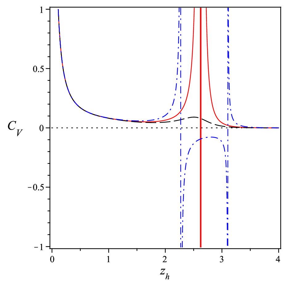
The behavior of temperature is shown in Figs. (11). In Fig. (11)a, the variation of temperature with respect to the horizon radius zhz_{h} for different values of the coupling of theory α\alpha is shown. As can be seen there exists a minimum temperature Tm​i​nT_{min} below which no black hole solution exist (thermal gas). However, for T>Tm​i​nT>T_{min}, there are two black hole solutions, a large and a small one (deconfined quark gluon plasma phase). The small black hole phase for which TT increases with zhz_{h} whereas the large black hole phase for which TT decreases with zhz_{h}. In Fig. (11)b, to study the stability of the solutions, we have shown the behavior of heat capacity CVC_{V} and temperature. As can be seen the large black hole has positive heat capacity and therefore is stable and small black hole is unstable and thus not physical.

Refer to caption
(a) ν=4.5,l=1,c=−0.5\nu=4.5,l=1,c=-0.5
Refer to caption
(b) ν=4.5,l=1,c=−0.5\nu=4.5,l=1,c=-0.5
Figure 11: Plots of TT in terms of zhz_{h} for α=0.1,0.2,0.3,0.4,0.5\alpha={\color[rgb]{1,0,0}0.1},{\color[rgb]{0,0,1}0.2},0.3,{\color[rgb]{0,1,0}0.4},{\color[rgb]{1,0.5,0}0.5} and ν=4.5\nu=4.5 (left). Plots of CVC_{V} and TT in terms of zhz_{h} for α=0.1,0.2,0.3,0.4,0.5\alpha={\color[rgb]{1,0,0}0.1},{\color[rgb]{0,0,1}0.2},0.3,{\color[rgb]{0,1,0}0.4},{\color[rgb]{1,0.5,0}0.5} (right)

Following the standard Bekenstein-Hawking formula (27), one can easily read the black hole entropy density ss, which is defined as

s=l3​e−3​c​zh244​zhν+1ν.s=\dfrac{l^{3}e^{-\frac{3cz_{h}^{2}}{4}}}{4z_{h}^{\frac{\nu+1}{\nu}}}. (52)

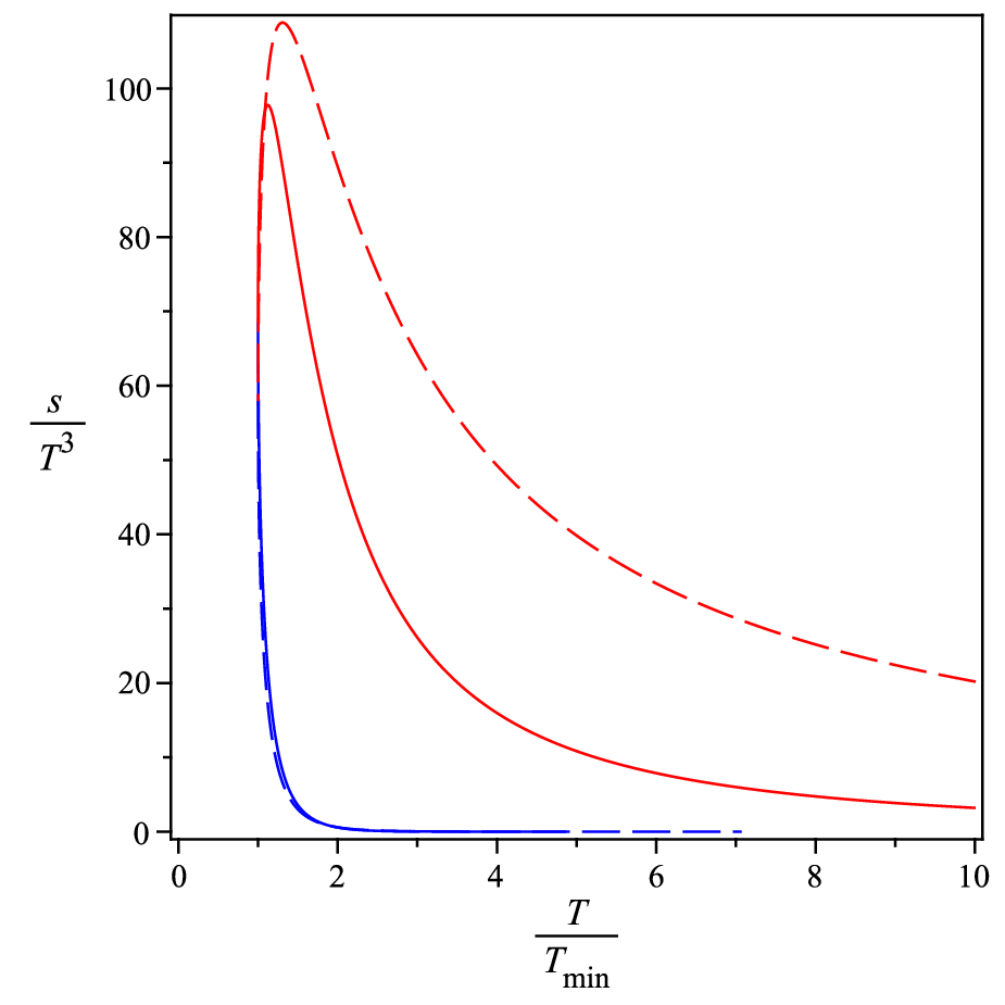
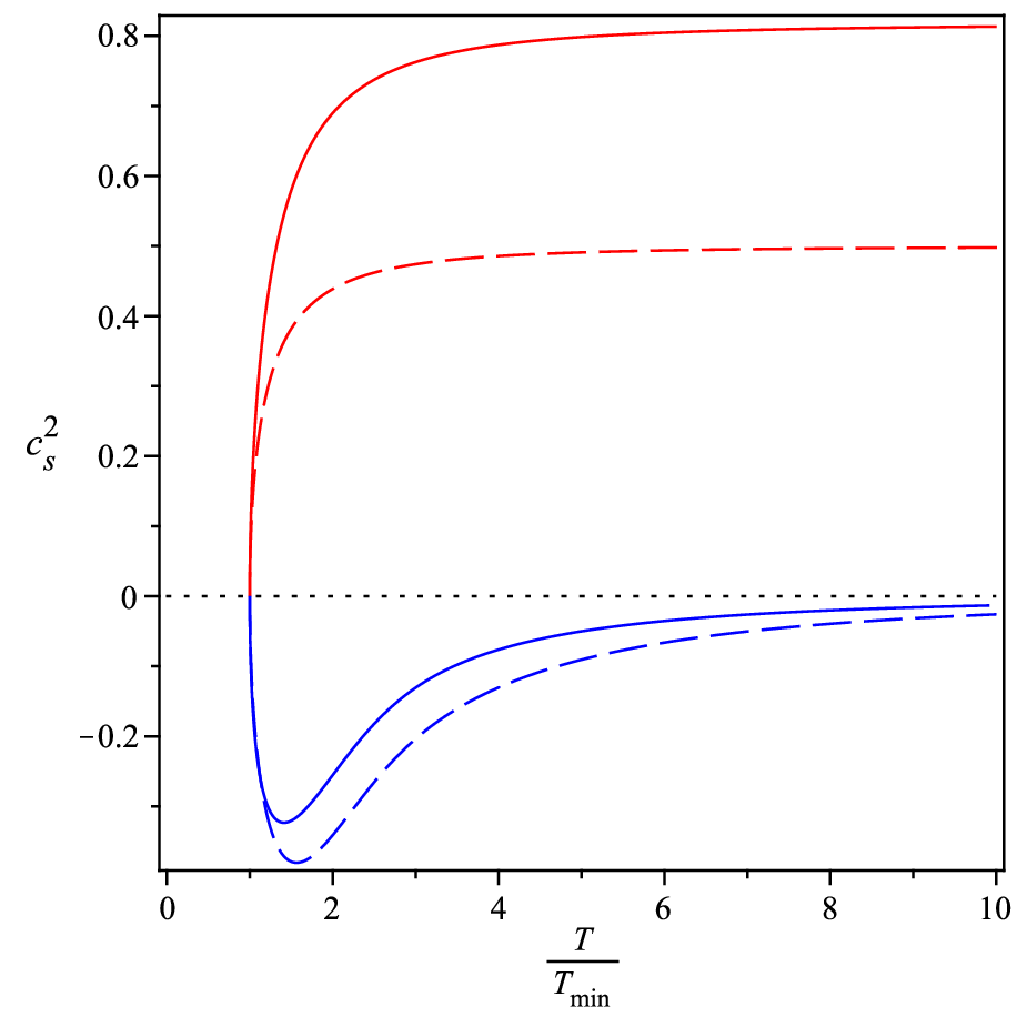
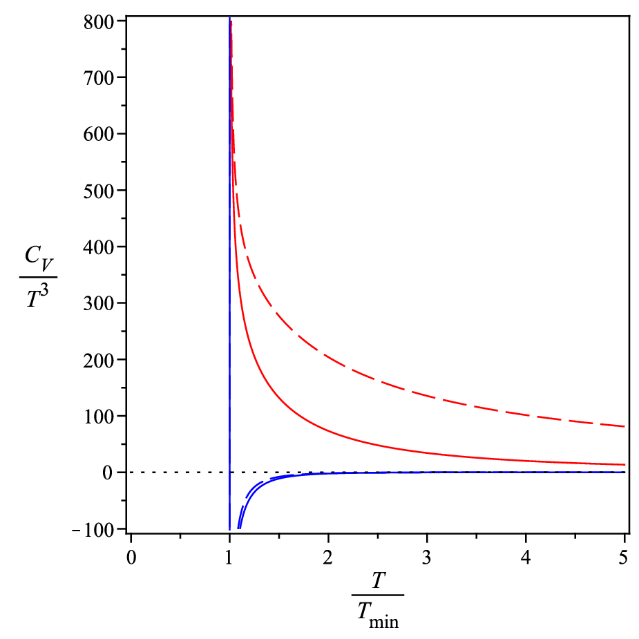
The scaled entropy density s/T3s/T^{3} as a function of scaled temperature T/Tm​i​nT/T_{min} is shown in Fig.12a. The red lines correspond to the large stable solution and blue lines are for the small unstable solution. The numerical result of the square of the sound velocity is shown in 12b. At Tm​i​nT_{min}, the sound velocity square is around 00 which is in agreement with lattice data 0.050.05. At high temperature, the sound velocity square goes to 0.450.45 for ν=1\nu=1, which means that the system is approximatly asymptotically conformal, while for ν=4.5\nu=4.5, the sound velocity square goes to 0.80.8. The numerical result of the specific heat is shown in Fig. 12c. It can be clearly seen that the specific heat CVC_{V} diverges at Tm​i​nT_{min}. At T→∞T\to\infty, the scaled specific heat CV/T3C_{V}/T^{3} approaches to the zero for this approximate solution [34].

Refer to caption
(a) l=1,c=−0.5,α=0.1l=1,c=-0.5,\alpha=0.1
Refer to caption
(b) l=1,c=−0.5,α=0.1l=1,c=-0.5,\alpha=0.1
Refer to caption
(c) l=1,c=−0.5,α=0.1l=1,c=-0.5,\alpha=0.1
Figure 12: Plots of scaled entropy density s/T3​(left),cs2​(middle)s/T^{3}\;(\text{left}),c_{s}^{2}\;(\text{middle}) and CV/T3​(right)C_{V}/T^{3}\;(\text{right}) in terms of scaled temperature T/Tm​i​nT/T_{min} for ν=1,Tm​i​n=0.19457​(dashed lines),ν=4.5,Tm​i​n=0.1357​(solid lines)\nu=1,T_{min}=0.19457\;(\text{dashed lines}),\nu=4.5,T_{min}=0.1357\;(\text{solid lines}). In each panel red lines correspond to the large stable solution and blue lines correspond to unstable small solution.

In figure 13, the behavior of cs2c_{s}^{2} and CVC_{V} have been shown. As can be seen from the figure and obtained the result in the previous section, it can be concluded that the heat capacity has an inverse relationship with the speed of sound.

Refer to caption
(a) l=1,c=−0.5,α=0.1l=1,c=-0.5,\alpha=0.1
Figure 13: Plots of cs2c_{s}^{2} (red lines) and CVC_{V} (blue lines) in terms of zhz_{h} for ν=1​(dashed lines),4.5​(solid lines)\nu=1\;(\text{dashed lines}),4.5\;(\text{solid lines}).

2.3 The case c≠0,μ≠0c\neq 0,\mu\neq 0

In this case the differential equation (2), becomes

4​ν​l​z2​e−c​z24​(l2​ν2​e−c​z22−α​(2+ν​c​z2)2​g​(z))​g′′−2​z​l​e−c​z24​(ν2​l2​(4+(2+3​z2)​ν)−CLOSE\displaystyle 4\nu lz^{2}e^{-\frac{cz^{2}}{4}}(l^{2}\nu^{2}e^{-\frac{cz^{2}}{2}}-\alpha(2+\nu cz^{2})^{2}g(z))g^{\prime\prime}-2zle^{-\frac{cz^{2}}{4}}(\nu^{2}l^{2}(4+(2+3z^{2})\nu)-
OPENα⁡(2+ν​c​z2)​(8+4​ν+6​ν​c​z2−6​c​ν2​z2+c2​ν2​z4)​g)​g′−4​α​ν​z2​l​e−c​z24​(2+ν​c​z2)2​g′2\displaystyle\alpha(2+\nu cz^{2})(8+4\nu+6\nu cz^{2}-6c\nu^{2}z^{2}+c^{2}\nu^{2}z^{4})g)g^{\prime}-4\alpha\nu z^{2}le^{-\frac{cz^{2}}{4}}(2+\nu cz^{2})^{2}g^{\prime 2}
−c2​ν3​l​𝔠22​z4​ν+2ν​ec​z24=0\displaystyle-c^{2}\nu^{3}l\mathfrak{c}_{2}^{2}z^{\frac{4\nu+2}{\nu}}e^{\frac{cz^{2}}{4}}=0 (53)

in order to solve the above differential equation, we assume

g⁡(z)=1+ϵ​g1​(z)+𝒪⁡(ϵ2),g(z)=1+\epsilon g_{1}(z)+\mathcal{O}(\epsilon^{2}), (54)

by inserting it, one can achieve a non-homogeneous differential equation as

g1′′+[−l2​ν3​(2+3​c​z2)−4​ν2​(l2+4​α​c​z2)+4​α​ν​(2+c​z2)+16​α]​g1′ν​z​(l2​ν2−4​α)+c​ν​𝔠22​z2ν​ec​z224​α​(4+c​ν​z2)=0.g_{1}^{\prime\prime}+\dfrac{[-l^{2}\nu^{3}(2+3cz^{2})-4\nu^{2}(l^{2}+4\alpha cz^{2})+4\alpha\nu(2+cz^{2})+16\alpha]g_{1}^{\prime}}{\nu z(l^{2}\nu^{2}-4\alpha)}+\dfrac{c\nu\mathfrak{c}_{2}^{2}z^{\frac{2}{\nu}}e^{\frac{cz^{2}}{2}}}{4\alpha(4+c\nu z^{2})}=0. (55)

In order to solve the non-homogeneous differential equation (55) in the case of c<0,𝔠2≠0c<0,\mathfrak{c}_{2}\neq 0, we consider the following particular solution:

g2​(z)=ec​z22​z−2​(ν−1)ν​∑ihi​zi,g_{2}(z)=e^{\frac{cz^{2}}{2}}z^{-\frac{2(\nu-1)}{\nu}}\sum_{i}h_{i}z^{i}, (56)

where hih_{i} are coefficients of expansions. By inserting the above solution into the differential equation (55), and solving order by order for coefficients, one can get

h0=h1=h3=h5=0,\displaystyle\hskip 142.26378pth_{0}=h_{1}=h_{3}=h_{5}=0,
h2\displaystyle h_{2} =𝔠22​ν28​α​(ν−2),h4=−c​ν3​𝔠22​(−20​α​ν+l2​ν3+l2​ν2−12​α)16​α​(ν−2)​(ν4​l2+3​l2​ν3−4​α​ν2+2​l2​ν2−12​α​ν−8​α),\displaystyle=\dfrac{\mathfrak{c}_{2}^{2}\nu^{2}}{8\alpha(\nu-2)},\;\;\;h_{4}=-\dfrac{c\nu^{3}\mathfrak{c}_{2}^{2}(-20\alpha\nu+l^{2}\nu^{3}+l^{2}\nu^{2}-12\alpha)}{16\alpha(\nu-2)(\nu^{4}l^{2}+3l^{2}\nu^{3}-4\alpha\nu^{2}+2l^{2}\nu^{2}-12\alpha\nu-8\alpha)},
h6\displaystyle h_{6} =ν4​c2​𝔠2232​α​(2+3​ν)​(l2​ν2−4​α)2​(1+2​ν)​(1+ν)​(ν2−4)​(3​l4​ν6+6​l5​ν5−40​ν4​l2​α+3​ν4​l4+256​α2​ν3CLOSE\displaystyle=\dfrac{\nu^{4}c^{2}\mathfrak{c}_{2}^{2}}{32\alpha(2+3\nu)(l^{2}\nu^{2}-4\alpha)^{2}(1+2\nu)(1+\nu)(\nu^{2}-4)}(3l^{4}\nu^{6}+6l^{5}\nu^{5}-40\nu^{4}l^{2}\alpha+3\nu^{4}l^{4}+256\alpha^{2}\nu^{3}
OPEN−56​ν3​l2​α+624​ν2​α2−24​ν2​l2​α+448​α2​ν+112​α2),\displaystyle-56\nu^{3}l^{2}\alpha+624\nu^{2}\alpha^{2}-24\nu^{2}l^{2}\alpha+448\alpha^{2}\nu+112\alpha^{2}), (57)

where 𝔠2\mathfrak{c}_{2} used from (11). Therefore, the metric function by considering a particular solution becomes

g⁡(z)=1−erf​(12​c⁡(−6​l2​ν2−32​ν​α+8​α)(l2​ν2−4​α)​z)erf​(12​c⁡(−6​l2​ν2−32​ν​α+8​α)(l2​ν2−4​α)​zh)+ec​z22​z−2​(ν−1)ν​∑ihi​zi,g(z)=1-\dfrac{\text{erf}\left(\dfrac{1}{2}\sqrt{\dfrac{c(-6l^{2}\nu^{2}-32\nu\alpha+8\alpha)}{(l^{2}\nu^{2}-4\alpha)}}z\right)}{\text{erf}\left(\dfrac{1}{2}\sqrt{\dfrac{c(-6l^{2}\nu^{2}-32\nu\alpha+8\alpha)}{(l^{2}\nu^{2}-4\alpha)}}z_{h}\right)}+e^{\frac{cz^{2}}{2}}z^{-\frac{2(\nu-1)}{\nu}}\sum_{i}h_{i}z^{i}, (58)

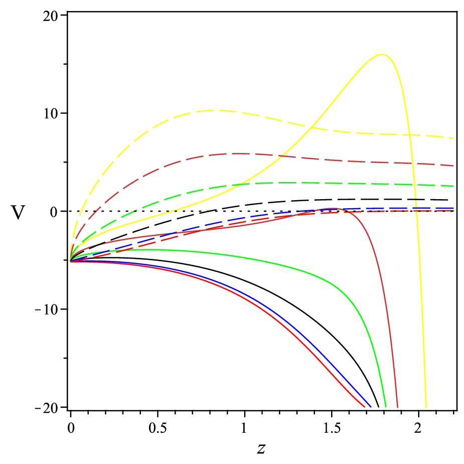
with hih_{i} are provided in (2.3). In figure 14, the effect of μ\mu on the behavior of f2f_{2} and VV have been shown. As can be seen in left panel by increasing chemical potential, f2f_{2} decreases and in right panel VV increases.

Refer to caption
(a) ν=4.5,l=1,α=0.1,c=±0.5\nu=4.5,l=1,\alpha=0.1,c=\pm 0.5
Refer to caption
(b) ν=4.5,l=1,α=0.1,c=±0.5\nu=4.5,l=1,\alpha=0.1,c=\pm 0.5
Figure 14: Plots of f2f_{2} and VV in terms of zz for μ=0,0.05,0.1,0.15,0.2,0.25\mu={\color[rgb]{1,0,0}0},{\color[rgb]{0,0,1}0.05},{\color[rgb]{0,0,0}0.1},{\color[rgb]{0,1,0}0.15},{\color[rgb]{1,0.5,0}0.2},{\color[rgb]{1,1,0}0.25}.
Refer to caption
(a) ν=4.5,l=1,c=−0.5,α=0.1\nu=4.5,l=1,c=-0.5,\alpha=0.1
Refer to caption
(b) ν=4.5,l=1,c=−0.5,α=0.1\nu=4.5,l=1,c=-0.5,\alpha=0.1
Refer to caption
(c) ν=4.5,l=1,c=−0.5,α=0.1\nu=4.5,l=1,c=-0.5,\alpha=0.1
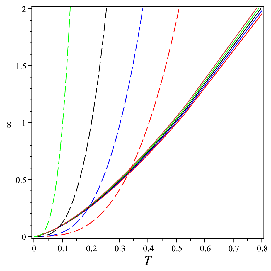
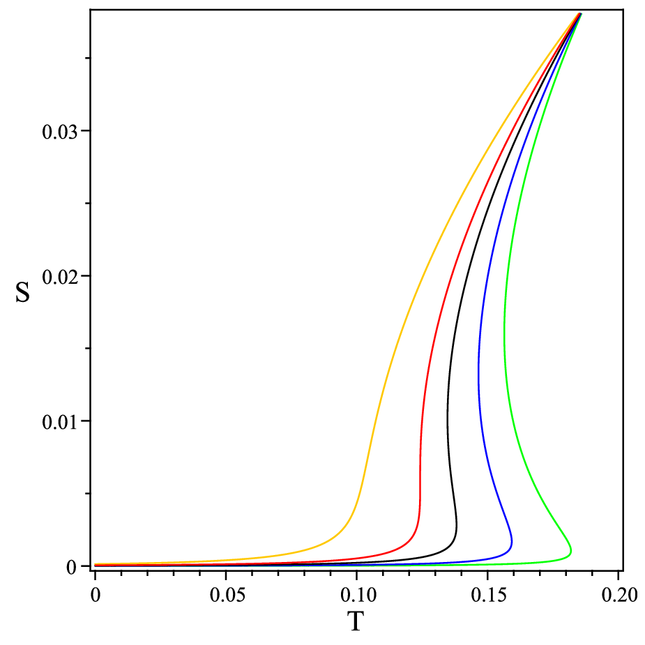
Figure 15: Plots of s,Ts,T and CVC_{V} in terms of zhz_{h} for μ=0.1,0.15,0.2,0.22728,0.3\mu={\color[rgb]{0,1,0}0.1},{\color[rgb]{0,0,1}0.15},{\color[rgb]{0,0,0}0.2},{\color[rgb]{1,0,0}0.22728},{\color[rgb]{1,0.5,0}0.3} (left) and μ=0.2,0.22728,0.3\mu={\color[rgb]{0,0,1}0.2},{\color[rgb]{1,0,0}0.22728},0.3 (middle and right).

In fig. 15a, the behavior of entropy is shown in terms of temperature. The figure shows the minimum and maximum temperature. As μ\mu increases, the minimum temperature decreases. This plot also shows that for 0<μ<μc0<\mu<\mu_{c}, there are minimal Tm​i​nT_{min} and maximal Tm​a​xT_{max} temperatures, between which the entropy is a function of TT with three branches. When we decrease the temperature, the entropy decreases along the first branch (Tm​i​n<T<∞T_{min}<T<\infty). Then the entropy decreases along the second branch with an increase of temperature from Tm​i​nT_{min} to Tm​a​xT_{max}, i.e. here the black holes are unstable. Finally the entropy increases along the third branch with an increase of temperature for 0<T<Tm​a​x0<T<T_{max}. Such a behavior in terms of event horizon, one can see in the 15b and c. In each panel, the critical point has been shown in red color curve. Upon varying the Hawking temperature, a phase transition from the large black hole phase to the thermal AdS phase takes place at a critical temperature Tc=0.1242T_{c}=0.1242. This is the famous black hole-thermal AdS Hawking-Page phase transition which occurs in the presence of chemical potential μc=0.22728\mu_{c}=0.22728. In fig. 16 by using the approximate analysis, the phase diagram of the holographic QCD model for anisotropic background and for Einstien gravity (long dashed line), Einstien-Gauss-Bonnet gravity (solid line) has been shown. As one can see at μ=0\mu=0 the system undergoes a black hole to thermal gas first order phase transition so that T(E​G​B)​(μ=0)>T(E)​(μ=0)T^{(EGB)}(\mu=0)>T^{(E)}(\mu=0). For 0<μ<μc0<\mu<\mu_{c} (in the transition lines), the system undergoes a large black hole to a small black hole first-order phase transition. For 0<μ<μI0<\mu<\mu_{I}, the temperature of the black hole to black hole transition of Einstien gravity (T(E)​(μ)T^{(E)}(\mu)) is less than Einstien-Gauss-Bonnet gravity (T(E​G​B)​(μ)T^{(EGB)}(\mu)) and for μI<μ<μc\mu_{I}<\mu<\mu_{c} vice versa. The first order phase transition stops at the critical point (μc,Tc\mu_{c},T_{c}), where the phase transition becomes second order, herewith Tc(E​G​B)<Tc(E)T^{(EGB)}_{c}<T^{(E)}_{c}, μc(E​G​B)<μc(E)\mu_{c}^{(EGB)}<\mu_{c}^{(E)}. For μ>μc\mu>\mu_{c}, the system has a sharp but smooth crossover. These thermal AdS and black hole phases in the usual language of gauge-gravity duality are dual to the confinement and deconfinement phases in the dual boundary theory.

Refer to caption
(a) ν=4.5,l=1,c=−0.5\nu=4.5,l=1,c=-0.5
Figure 16: The phase diagram in TT and μ\mu plane for anisotropic background. At small μ\mu, the system undergoes a first order phase transition at finite TT. The first order phase transition stops at the critical point (μc,Tc)∼(0.22728,0.1242)(\mu_{c},T_{c})\sim(0.22728,0.1242), where the phase transition becomes second order. The solid line is for α=0.1\alpha=0.1 and long dashed line is for α=0\alpha=0.

3 Conclusion

In this work, we extended the AdS/QCD model to quadratic gravity to gain insight into the influence of gravity on QCD. To do so, we considered an anisotropic black hole metric as a solution to a system of 5​D5D Einstein-quadratic-two Maxwell-dilaton fields. The anisotropic background is specified by an arbitrary exponent, a non-zero dilaton field, a non-zero time component of the first Maxwell field, and a non-zero longitudinal magnetic component of the second Maxwell field. The field equations for the considered theory are coupled and bulky differential equations for six unknown functions. Therefore, obtaining the solution to such field equations is too hard, this is why we considered the special case of field equation, i.e. γ=α,β=−4​α\gamma=\alpha,\beta=-4\alpha (Einstien-Gauss-Bonnet gravity). The differential equation for the metric function in EGB gravity is a nonlinear second-order equation that has been solved in special cases. At the first, we obtained the exact solutions for the differential equations with zero warp functions. In this case, it doesn’t occur any thermodynamical phase transitions to the black brane. The second case that we have considered is the case with zero chemical potential. The blackening function in this case supports the Van der Waals-like phase transition between small and large black holes for suitable values of parameters. The third case that has been considered is nonzero warp function and chemical potential. In this case, in addition to the small/large phase transition, the blackening function supported the phase transition from the large black hole phase to the thermal AdS phase at a critical temperature. Holographically, this phase transition corresponds to the confinement-deconfinement phase transition in QCD. In each case, we investigated the anisotropy influence and the effect of parameters of theory on the thermodynamic properties of our background, in particular, on the small/large black holes phase transition diagram. In fig. (16), the effect of the Gauss-Bonnet term on the phase transition has been shown. This figure shows that before/after the intersection point for constant chemical potential, the temperature of a black hole in EGB gravity is more/less than that of Einstien gravity. Clearly, before the intersection point, α\alpha has a dominant impact on the temperature (compared to the effect of μ\mu on the temperature). In the isotropic case corresponding to ν=1\nu=1 (zero magnetic fields) and ,α→0,\alpha\to 0 reproduces previously known results [8].
For future work, one can consider the Weyl-squared term by using the combination γ=6​α\gamma=6\alpha and β=−4/3γ\beta=-4/3\gamma for the parameters of the theory. But since in this case, the field equation for the metric has a 4th-order derivative, the differential equations should be solved numerically. Also, following the paper [9], one can study the effect of the magnetic field on the system in the framework of EGB.

Acknowledgements

I would like to thank the referee for her/his fruitful comments. I also would like to thank the School of Physics of the Institute for Research in Fundamental Sciences (IPM).

Constants

The constants related to equation(19):

ℰ\displaystyle\mathcal{E} =(ν+1)​((ν+1)​(ν4​l4−8​α​c2)−4​α​ν​c1​z2​ν+2ν),\displaystyle=(\nu+1)((\nu+1)(\nu^{4}l^{4}-8\alpha c_{2})-4\alpha\nu c_{1}z^{\frac{2\nu+2}{\nu}}),
𝒟\displaystyle\mathcal{D} =ν​l2−ν2​l2−ν4​l4−8​α​c2,\displaystyle=\nu l^{2}-\nu^{2}l^{2}-\sqrt{\nu^{4}l^{4}-8\alpha c_{2}},
ℱ\displaystyle\mathcal{F} =ν​l2−ν2​l2+ν4​l4−8​α​c2,\displaystyle=\nu l^{2}-\nu^{2}l^{2}+\sqrt{\nu^{4}l^{4}-8\alpha c_{2}},
𝒢\displaystyle\mathcal{G} =ν3​l2−ν​l2−ℰν+1,\displaystyle=\dfrac{\nu^{3}l^{2}-\nu l^{2}-\sqrt{\mathcal{E}}}{\nu+1},
ℋ\displaystyle\mathcal{H} =−l2​ν​(ν−1)​ν4​l4−8​α​c2+ν4​l4−8​α​c2,\displaystyle=-l^{2}\nu(\nu-1)\sqrt{\nu^{4}l^{4}-8\alpha c_{2}}+\nu^{4}l^{4}-8\alpha c_{2},
𝒦\displaystyle\mathcal{K} =−l2​ν​(ν−12)​ℰ−2​α​c1​ν​z2​ν+2ν+(ν+1)​(ν4​l4−4​α​c2−l4​ν32),\displaystyle=-l^{2}\nu\left(\nu-\frac{1}{2}\right)\sqrt{\mathcal{E}}-2\alpha c_{1}\nu z^{\frac{2\nu+2}{\nu}}+(\nu+1)\left(\nu^{4}l^{4}-4\alpha c_{2}-\dfrac{l^{4}\nu^{3}}{2}\right),
ℒ\displaystyle\mathcal{L} =l2​ν​(ν−1)​ν4​l4−8​α​c2+ν4​l4−8​α​c2.\displaystyle=l^{2}\nu(\nu-1)\sqrt{\nu^{4}l^{4}-8\alpha c_{2}}+\nu^{4}l^{4}-8\alpha c_{2}. (59)

The constants related to equation(2.1):

𝒜¯\displaystyle\bar{\mathcal{A}} =(ν+1)​(−4​α​c1​ν​z2​ν+2ν+(ν+1)​(ν4​l4−8​α​c2)),\displaystyle=(\nu+1)(-4\alpha c_{1}\nu z^{\frac{2\nu+2}{\nu}}+(\nu+1)(\nu^{4}l^{4}-8\alpha c_{2})),
ℬ¯\displaystyle\bar{\mathcal{B}} =−4​α​ν2​c1​z2​ν+2ν+(ν+1)​(ν+32)​(ν4​l4−8​α​c2),\displaystyle=-4\alpha\nu^{2}c_{1}z^{\frac{2\nu+2}{\nu}}+(\nu+1)(\nu+\frac{3}{2})(\nu^{4}l^{4}-8\alpha c_{2}),
𝒞¯\displaystyle\bar{\mathcal{C}} =−4​α​ν​c1​z2​ν+2ν+(ν+1)​(ν4​l4−8​α​c2),\displaystyle=-4\alpha\nu c_{1}z^{\frac{2\nu+2}{\nu}}+(\nu+1)(\nu^{4}l^{4}-8\alpha c_{2}),
ℰ¯\displaystyle\bar{\mathcal{E}} =−4​c12​α2​ν2​(3​ν3−4​ν2+3​ν+2)​z2​(2​ν+2)ν+\displaystyle=-4c_{1}^{2}\alpha^{2}\nu^{2}(3\nu^{3}-4\nu^{2}+3\nu+2)z^{\frac{2(2\nu+2)}{\nu}}+
2​c1​ν​α​(ν2−1)​(ν4​l4+2​l4​ν3−16​α​ν​c2−8​α​c2)​z2​ν+2ν+\displaystyle 2c_{1}\nu\alpha(\nu^{2}-1)(\nu^{4}l^{4}+2l^{4}\nu^{3}-16\alpha\nu c_{2}-8\alpha c_{2})z^{\frac{2\nu+2}{\nu}}+
(ν−1)​(ν+1)2​(ν4​l4−8​α​c2)​(4​α​c2+ν5​l5−l4​ν3−ν4​l42),\displaystyle(\nu-1)(\nu+1)^{2}(\nu^{4}l^{4}-8\alpha c_{2})(4\alpha c_{2}+\nu^{5}l^{5}-l^{4}\nu^{3}-\frac{\nu^{4}l^{4}}{2}),
ℱ¯\displaystyle\bar{\mathcal{F}} =ν7​l4−72​ν6​l4+2​ν5​l4+52​ν4​l4+4​ν3​α​c2+24​α​ν2​c2−36​α​ν​c2−8​α​c2,\displaystyle=\nu^{7}l^{4}-\frac{7}{2}\nu^{6}l^{4}+2\nu^{5}l^{4}+\frac{5}{2}\nu^{4}l^{4}+4\nu^{3}\alpha c_{2}+24\alpha\nu^{2}c_{2}-36\alpha\nu c_{2}-8\alpha c_{2},
ℋ¯\displaystyle\bar{\mathcal{H}} =4​c12​α2​(5​ν+2−2​ν2+ν3)​z2​(2​ν+2)ν−4​c1​α​(ν2−1)​(l4​ν3−8​α​ν​c2+4​α​c2)​z2​ν+2ν\displaystyle=4c_{1}^{2}\alpha^{2}(5\nu+2-2\nu^{2}+\nu^{3})z^{\frac{2(2\nu+2)}{\nu}}-4c_{1}\alpha(\nu^{2}-1)(l^{4}\nu^{3}-8\alpha\nu c_{2}+4\alpha c_{2})z^{\frac{2\nu+2}{\nu}}
−(ν+1)2​(ν−1)​ν2​l4​(ν2−12​ν−1)​(ν4​l4−8​α​c2),\displaystyle-(\nu+1)^{2}(\nu-1)\nu^{2}l^{4}(\nu^{2}-\frac{1}{2}\nu-1)(\nu^{4}l^{4}-8\alpha c_{2}),
𝒢¯\displaystyle\bar{\mathcal{G}} =ν5​l4+2​α​c2+12​ν4​l4−12​ν3​l4,𝒦¯=ν5​l4+13​ν4​l4−12​l4​ν3+4​α​c2,\displaystyle=\nu^{5}l^{4}+2\alpha c_{2}+\frac{1}{2}\nu^{4}l^{4}-\frac{1}{2}\nu^{3}l^{4},\;\;\;\;\;\bar{\mathcal{K}}=\nu^{5}l^{4}+\frac{1}{3}\nu^{4}l^{4}-\frac{1}{2}l^{4}\nu^{3}+4\alpha c_{2},
ℒ¯\displaystyle\bar{\mathcal{L}} =576​α2​c22​𝒢¯​𝒞¯+12​𝒜¯2​ℋ¯,𝒥¯=320​α2​c22​𝒢¯​𝒞¯−12​(𝒜¯2​(𝒜¯​ℬ¯−ℋ¯)).\displaystyle=576\alpha^{2}c_{2}^{2}\bar{\mathcal{G}}\bar{\mathcal{C}}+\frac{1}{2}\bar{\mathcal{A}}^{2}\bar{\mathcal{H}},\;\;\;\;\bar{\mathcal{J}}=320\alpha^{2}c_{2}^{2}\bar{\mathcal{G}}\bar{\mathcal{C}}-\frac{1}{2}(\bar{\mathcal{A}}^{2}(\bar{\mathcal{A}}\bar{\mathcal{B}}-\bar{\mathcal{H}})). (60)

References

  • [1] J. M. Maldacena, Adv. Theor. Math. Phys. 2, 231-252 (1998) doi:10.1023/A:1026654312961 [arXiv:hep-th/9711200 [hep-th]].
  • [2] E. Witten, Adv. Theor. Math. Phys. 2, 253-291 (1998) doi:10.4310/ATMP.1998.v2.n2.a2 [arXiv:hep-th/9802150 [hep-th]].
  • [3] J. Casalderrey-Solana, H. Liu, D. Mateos, K. Rajagopal and U. A. Wiedemann, Cambridge University Press, 2014, ISBN 978-1-139-13674-7 doi:10.1017/CBO9781139136747 [arXiv:1101.0618 [hep-th]].
  • [4] I. Y. Aref’eva, Phys. Usp. 57, 527-555 (2014) doi:10.3367/UFNe.0184.201406a.0569
  • [5] M. Strickland, Pramana 84, no.5, 671-684 (2015) doi:10.1007/s12043-015-0972-1 [arXiv:1312.2285 [hep-ph]].
  • [6] O. Andreev and V. I. Zakharov, Phys. Rev. D 74, 025023 (2006) doi:10.1103/PhysRevD.74.025023 [arXiv:hep-ph/0604204 [hep-ph]].
  • [7] S. He, S. Y. Wu, Y. Yang and P. H. Yuan, JHEP 04, 093 (2013) doi:10.1007/JHEP04(2013)093 [arXiv:1301.0385 [hep-th]].
  • [8] I. Aref’eva and K. Rannu, JHEP 05, 206 (2018) doi:10.1007/JHEP05(2018)206 [arXiv:1802.05652 [hep-th]].
  • [9] H. Bohra, D. Dudal, A. Hajilou and S. Mahapatra, Phys. Lett. B 801, 135184 (2020) doi:10.1016/j.physletb.2019.135184 [arXiv:1907.01852 [hep-th]].
  • [10] Z. Y. Fan and H. Lu, Phys. Rev. D 91, no.6, 064009 (2015) doi:10.1103/PhysRevD.91.064009 [arXiv:1501.00006 [hep-th]].
  • [11] S. N. Sajadi and S. H. Hendi, Eur. Phys. J. C 82, no.8, 675 (2022) doi:10.1140/epjc/s10052-022-10647-9 [arXiv:2207.13435 [gr-qc]].
  • [12] S. N. Sajadi, R. B. Mann, N. Riazi and S. Fakhry, doi:10.1103/PhysRevD.102.124026 [arXiv:2010.15039 [gr-qc]].
  • [13] S. N. Sajadi, A. Hajilou and S. H. Hendi, [arXiv:2208.09892 [gr-qc]].
  • [14] S. N. Sajadi, L. Shahkarami, F. Charmchi and S. H. Hendi, [arXiv:2207.07374 [gr-qc]].
  • [15] S. Ferrara, R. R. Khuri and R. Minasian, Phys. Lett. B 375, 81-88 (1996) doi:10.1016/0370-2693(96)00270-5 [arXiv:hep-th/9602102 [hep-th]].
  • [16] D. M. Hofman, Nucl. Phys. B 823, 174-194 (2009) doi:10.1016/j.nuclphysb.2009.08.001 [arXiv:0907.1625 [hep-th]].
  • [17] M. Brigante, H. Liu, R. C. Myers, S. Shenker and S. Yaida, Phys. Rev. D 77, 126006 (2008) doi:10.1103/PhysRevD.77.126006 [arXiv:0712.0805 [hep-th]].
  • [18] J. de Boer, M. Kulaxizi and A. Parnachev, JHEP 03, 087 (2010) doi:10.1007/JHEP03(2010)087 [arXiv:0910.5347 [hep-th]].
  • [19] X. O. Camanho and J. D. Edelstein, JHEP 06, 099 (2010) doi:10.1007/JHEP06(2010)099 [arXiv:0912.1944 [hep-th]].
  • [20] C. Garraffo and G. Giribet, Mod. Phys. Lett. A 23, 1801-1818 (2008) doi:10.1142/S0217732308027497 [arXiv:0805.3575 [gr-qc]].
  • [21] C. Charmousis, Lect. Notes Phys. 769, 299-346 (2009) doi:10.1007/978-3-540-88460-6_8 [arXiv:0805.0568 [gr-qc]].
  • [22] F. Canfora, A. Cisterna, S. Fuenzalida, C. Henriquez-Baez and J. Oliva, Phys. Rev. D 104, no.4, 044026 (2021) doi:10.1103/PhysRevD.104.044026 [arXiv:2103.09110 [hep-th]].
  • [23] N. Deruelle and J. Madore, [arXiv:gr-qc/0305004 [gr-qc]].
  • [24] B. Zwiebach, Phys. Lett. B 156, 315-317 (1985) doi:10.1016/0370-2693(85)91616-8
  • [25] P. Kanti and K. Tamvakis, Phys. Rev. D 52, 3506-3511 (1995) doi:10.1103/PhysRevD.52.3506 [arXiv:hep-th/9504031 [hep-th]].
  • [26] S. O. Alexeev and M. V. Pomazanov, Phys. Rev. D 55, 2110-2118 (1997) doi:10.1103/PhysRevD.55.2110 [arXiv:hep-th/9605106 [hep-th]].
  • [27] P. Kanti, N. E. Mavromatos, J. Rizos, K. Tamvakis and E. Winstanley, Phys. Rev. D 57, 6255-6264 (1998) doi:10.1103/PhysRevD.57.6255 [arXiv:hep-th/9703192 [hep-th]].
  • [28] T. Padmanabhan and D. Kothawala, Phys. Rept. 531, 115-171 (2013) doi:10.1016/j.physrep.2013.05.007 [arXiv:1302.2151 [gr-qc]].
  • [29] G. W. Horndeski, Int. J. Theor. Phys. 10, 363-384 (1974) doi:10.1007/BF01807638
  • [30] T. Kobayashi, Rept. Prog. Phys. 82, no.8, 086901 (2019) doi:10.1088/1361-6633/ab2429 [arXiv:1901.07183 [gr-qc]].
  • [31] P. G. S. Fernandes, P. Carrilho, T. Clifton and D. J. Mulryne, Class. Quant. Grav. 39, no.6, 063001 (2022) doi:10.1088/1361-6382/ac500a [arXiv:2202.13908 [gr-qc]].
  • [32] R. M. Wald, Phys. Rev. D 48, no. 8, R3427 (1993) doi:10.1103/PhysRevD.48.R3427 [gr-qc/9307038].
  • [33] V. Iyer and R. M. Wald, Phys. Rev. D 50, 846 (1994) doi:10.1103/PhysRevD.50.846 [gr-qc/9403028].
  • [34] D. Li, S. He, M. Huang and Q. S. Yan, JHEP 09, 041 (2011) doi:10.1007/JHEP09(2011)041 [arXiv:1103.5389 [hep-th]].