Integral Micromorphic Model for Band Gap in 1D Continuum

The free energy density function for the local micromorphic model introduced in equation (1) is now generalized to include nonlocal effects both in the coupling term $\varphi(\varepsilon)$ and in the strain-related term. The generalized expression reads

where ${\cal L}$ is the one-dimensional domain representing the analyzed body (here we consider ${\cal L}=(-\infty,\infty)$), $\alpha_{0}$ and $\alpha_{1}$ are nonlocal averaging kernels and $A$ is the generalized micromorphic modulus. Parameter $H$ can be interpreted as a penalty coefficient; in the limit case when $H\to\infty$, the micromorphic variable corresponds to the nonlocal strain evaluated with weight function $\alpha_{1}$, and the presented model simplifies to the higher-order nonlocal strain gradient elasticity which was introduced in [15] and studied in [14]. For simplicity, we do not mark explicitly that the state variables in general depend not only on the spatial coordinate but also on time, $t$.

It would also be possible to introduce spatial averaging for inertia, however, this modification is not considered here, and the kinetic energy is generalized only in the micromorphic sense, i.e., its density is given by

where $\rho$ is the standard mass density and $\eta$ is a nonstandard, micromorphic density. The superimposed dot denotes a derivative with respect to time.

In the spirit of the Hamilton principle, we define the action functional

and set its first variation to zero, assuming that the state of the system at times $t_{1}$ and $t_{2}$ is fixed. Substituting from (2)–(3) with $\varepsilon$ replaced by $u^{\prime}$, evaluating the variation, integrating by parts with respect to time and taking into account that the variations at $t_{1}$ and $t_{2}$ vanish, we obtain the stationarity condition

in which

can be interpreted as the stress, the higher-order stress, and the relative stress.

Condition (5) should be satisfied for all admissible variations $\delta u$ and $\delta\chi$. Integrating the terms with $\delta u^{\prime}$ and $\delta\chi^{\prime}$ by parts with respect to space, we end up with Euler-Lagrange equations

Note that expression (6) for $\Sigma$ contains a double integral, but integration with respect to $\eta$ can be done in advance because it does not involve the variable fields. Denoting

we can rewrite (6) as

The resulting equations of motion deduced from (9)–(10) read

Function $E_{H}$ defined in (11) is a modified weight function, which turns out to be symmetric with respect to $x$ and $\xi$ even if the original functions $E(x,\xi)$ and $\alpha_{1}(x,\xi)$ are not. If this weight function depends only on the distance, i.e., if $E_{H}(x,\xi)=E_{0}(x-\xi)$, then the “outer derivative” on the right-hand side of (13) can be “shifted” into the nonlocal integrals (for simplicity, we drop the dependence on the time variable):

Here we have used certain assumed properties of the weight function, e.g., $E_{0}(r)\to 0$ as $|r|\to\infty$. If the weight function $\alpha_{1}$ also depends just on the distance, one can show by an analogous procedure that

and equation (13) can then be rewritten as

The dispersion equation, i.e., the relation between circular frequency $\omega$ and wave number $k$, is now derived by assuming harmonic propagation of both displacement and micromorphic variable. For an infinite and macroscopically homogeneous body, it is natural to expect that the weight functions depend on distance only. With a slight abuse of notation, we will write $\alpha_{j}(x-\xi)$ instead of $\alpha_{j}(x,\xi)$, $j=0,1$, and also $E_{H}(x-\xi)$ instead of $E_{H}(x,\xi)$. Plugging the harmonic ansatz

into equations (17) and (14) and multiplying both equations by ${\rm e}^{-i(kx-\omega t)}$ leads to conditions

which can be written in a matrix form as

where $\alpha^{*}_{j}(k)=\int_{\cal L}\alpha_{j}(r){\rm e}^{-ikr}{\rm d}r$, $j=0,1$, denotes the Fourier transform of the $j$-th nonlocal kernel. It is worth noting that since ${\cal L}=(-\infty,\infty)$ and the weight function $\alpha_{j}$ is always even, the imaginary part of $\alpha_{j}^{*}$ vanishes. Therefore, $\alpha_{j}^{*}$ can also be defined by the cosine Fourier transform

A nontrivial solution of homogeneous linear algebraic equations (20) exists if and only if the determinant of the matrix vanishes. This condition results in the dispersion equation

where $C^{*}(k)=E\alpha_{0}^{*}(k)+H\alpha_{1}^{*2}(k)$. This is a quadratic equation in terms of $\omega^{2}$ and its solution reads

For $C^{*}(k)=E+H$ and $\alpha_{1}^{*}(k)=1$, this reduces to the dispersion relation

valid for the “local” micromorphic model, i.e., for the model with the free energy density given by (1) with $\varphi(\varepsilon)\equiv\varepsilon$.

Since we are dealing with 5 model parameters ($E$, $A$, $H$, $\rho$, and $\eta$) that have 3 independent units, we can reduce the description to $5-3=2$ dimensionless input parameters. Our choice here is to consider $\kappa=H/E$ and $\lambda^{2}=A\rho/(E\eta)$. Therefore, in the dimensionless format, $\rho$, $\eta$, and $E$ are replaced by 1, $H$ is replaced by $\kappa$, and $A$ by $\lambda^{2}$. The wave number $k$ and circular frequency $\omega$ will be transformed into their dimensionless counterparts $\tilde{k}=k\sqrt{\eta/\rho}$ and $\tilde{\omega}=\omega\sqrt{\eta/E}$. The physical meaning of parameter $\lambda$ will become clear later (it is the ratio of the speed of fictitious “purely micromorphic” waves that would appear in a fully decoupled local model with $H=0$ and the standard elastic wave speed).

In the one-dimensional setting, the kernels $\alpha_{j}$ have units 1/m, and so we can convert them into dimensionless kernels $\tilde{\alpha}_{j}=\alpha_{j}\sqrt{\eta/\rho}$ and perform averaging by integrating with respect to the dimensionless spatial coordinate $\tilde{x}=x\sqrt{\rho/\eta}$. The Fourier image $\alpha_{j}^{*}$ is dimensionless but it is considered as function of the wave number $k$, which has units 1/m. Therefore, we will introduce the symbol $\tilde{\alpha}_{j}^{*}$ for the Fourier transform as function of the dimensionless wave number $\tilde{k}$. To explain that better, let us look at the following transformation (for convenience, we introduce an auxiliary length parameter $\ell=\sqrt{\eta/\rho}$):

It should be noted that the definition of the kernel typically involves at least one length-scale parameter. For instance, the Gaussian kernel

has length parameter $a$, and the corresponding Fourier transform is

The dimensionless counterparts

contain a dimensionless parameter $\tilde{a}=a/\ell$ where $\ell=\sqrt{\eta/\rho}$ is the length scale already set by other parameters of the model, $\eta$ and $\rho$. Now it is easy to rewrite the dispersion relation (23) in the dimensionless form

The positive sign before the square root corresponds to the optical branch and the negative one to the acoustic branch.

The local dimensionless formulation can be recovered from the nonlocal model by setting both averaging kernels $\tilde{\alpha}_{0}(\tilde{x})$ and $\tilde{\alpha}_{1}(\tilde{x})$ to the Dirac delta distribution. Consequently, the associated Fourier images $\tilde{\alpha}^{*}_{0}(\tilde{k})$ and $\tilde{\alpha}^{*}_{1}(\tilde{k})$ are set to 1 and the local counterpart to equation (30) reads

For $\tilde{k}=0$, i.e., in the long-wave limit, the corresponding frequency is given by

which means that the frequency on the acoustic branch is 0 and on the optical branch it is $\sqrt{\kappa}$. Therefore, parameter $\kappa$ controls the initial value on the optical branch. This is also valid for the general nonlocal model because $\tilde{\alpha}^{*}(0)=1$ for any weight function satisfying the normalizing condition $\int_{\cal L}\alpha(\xi)\,\mbox{d}\xi=1$.

In the opposite extreme case, for $\tilde{k}\to\infty$, i.e., in the short-wave limit, the dispersion relation can be approximated by

This means that the optical branch asymptotically approaches a straight line of slope $\max(\lambda,\sqrt{1+\kappa})$ and the acoustic branch a straight line of slope $\min(\lambda,\sqrt{1+\kappa})$. This terminal slope represents the dimensionless speed of very short waves (i.e., the actual speed normalized by the standard elastic wave speed, $c_{0}=\sqrt{E/\rho}$). On the other hand, the dimensionless speed of very long acoustic waves is represented by the initial slope of the acoustic branch and is always equal to 1, which corresponds to standard elasticity. This is natural, because if the wavelength is much larger than the internal length of the enriched continuum, the enrichment effect becomes negligible.

The effect of parameter $\kappa$ is illustrated by the dispersion curves in Figure 1. In the theoretical limit case when $\kappa=0$ (i.e., when $H=0$), equation (31) yields

This indicates that if the coupling between the micromorphic variable and the strain is not enforced (i.e., the penalty parameter $H$ is set to zero), the two branches of the dimensionless dispersion curve reduce to two straight lines with slopes 1 and $\lambda$, resp., both starting at the origin. The branch with slope 1 corresponds to the standard elasticity theory, and the branch with slope $\lambda$ is artificial, because the micromorphic variable is for $H=0$ totally independent of displacement or strain. However, the artificial branch indicates what can be expected for the optical branch in the case of weak coupling with a small but nonzero value of penalty parameter $H$ (note the blue curves with hollow circles, corresponding to $\kappa=0.2$). Also, this analysis confirms the previously announced interpretation of parameter $\lambda$ as the ratio between two wave speeds—one is the speed $\sqrt{A/\eta}$ of fictitious “micromorphic waves” that would arise for a model with no coupling between the micromorphic variable and strain, and the other is the standard elastic wave speed, $\sqrt{E/\rho}$.

In the opposite limit case when $\kappa\to\infty$ (i.e., $H\to\infty$, resulting into a strongly coupled model), the micromorphic variable $\chi$ coincides with the strain $\varepsilon$ and the model reduces to strain gradient elasticity with higher-order inertia, which was introduced in [32] by Metrikine & Askes. The corresponding dimensionless dispersion relation reads

and in Figure 1 it is plotted in brown. The optical branch in this limit case disappears—it blows up to infinity.

Note that the dispersion curves in Figure 1(a) are plotted for a fixed value of $\lambda=0.5<1$ and in Figure 1(b) for a fixed value of $\lambda=2>1$. In the former case, $\lambda<\sqrt{1+\kappa}$ for all meaningful (non-negative) values of $\kappa$, and so all the acoustic branches have the same terminal slope, given by $\lambda$, while the optical branches have terminal slopes that increase with $\kappa$ and are given by $\sqrt{1+\kappa}$; see Figure 1(a). In the latter case (i.e., $\lambda=2$), the acoustic branches for $\kappa<3$ have terminal slope $\sqrt{1+\kappa}$, increasing with $\kappa$, and for all $\kappa\geq 3$ they have the same terminal slope 2; see Figure 1(b). The optical branches have the same terminal slope 2 for $\kappa\leq 3$ and their slope increases with increasing $\kappa$ for $\kappa>3$. In all cases discussed here, the acoustic branch keeps rising to infinity as $\tilde{k}\to\infty$, and so there can be no band gap.

The influence of parameter $\lambda$ is illustrated in Figure 2 for a fixed value of $\kappa=4$. All the optical branches start from the same point at frequency $\tilde{\omega}_{0}=\sqrt{\kappa}=2$. If $\lambda$ increases but remains below $\sqrt{1+\kappa}=\sqrt{5}$, the terminal slope of the acoustic branch is given by $\lambda$ and thus increases, while the terminal slope of the optical branch remains constant, equal to $\sqrt{5}$. For higher values of $\kappa$, the terminal slope of all acoustic branches is the same and equal to $\sqrt{5}$ while the terminal slope of the optical branch increases with increasing $\lambda$.

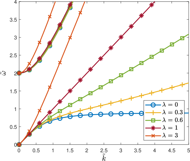
Interesting behavior can be observed when $\lambda=0$. This is the only case in which the acoustic branch has a finite limit $\sqrt{\kappa/(1+\kappa)}$ for large wave numbers $\tilde{k}$. Since the optical branch always starts at $\tilde{\omega}_{0}=\sqrt{\kappa}$ and the frequency on this branch increases with increasing wave number, a band gap in the dispersion diagram appears; see the blue curves with circular markers in Figure 2. This case corresponds to a vanishing micromorphic modulus $A$ and therefore to a model with micromorphic density only, not accompanied by any micromorphic stiffness.

Another special case arises when $\lambda=1$, because then the acoustic branch becomes a straight line of slope 1, which happens to be the same as for standard local elasticity, but there exists also an optical branch, given by $\tilde{\omega}=\sqrt{\kappa+(1+\kappa)\tilde{k}^{2}}$. For $\lambda<1$, the acoustic branch is concave, and for $\lambda>1$ it is convex. The optical branch is always convex.

In the previous subsection it was demonstrated that, for the local micromorphic model, a band gap in the one-dimensional dispersion curve appears only when the micromorphic modulus $A$ vanishes (and the micromorphic density parameter, $\eta$, is positive). In the following, the general integral micromorphic model introduced in Section 2 is considered and the added value of nonlocal averaging is analyzed.

Three typical nonlocal weight functions are considered here; their definitions and the corresponding Fourier images are summarized in Table 1 and graphically represented in Figure 3 for chosen length scale parameter $a=\ell$ (i.e., $\tilde{a}=1$). The Gaussian weight function as well as the exponential one have an unbounded support and a strictly positive Fourier image, while the quartic polynomial weight function vanishes for $\tilde{x}>\tilde{a}$ and its Fourier image has negative values in certain intervals of the wave number, the first one being $\tilde{k}\in(5.763,9.095)$.

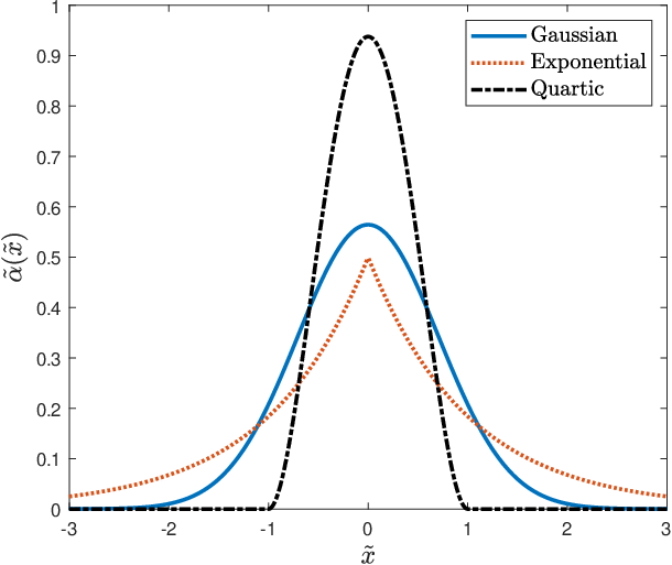
Let us firstly investigate the asymptotic behavior of the dispersion relation when $\tilde{k}\to\infty$ (i.e., in the short-wave limit). For all nonlocal kernels listed in Table 1, the product $\tilde{k}{\tilde{\alpha}^{*}}(\tilde{k})$ tends to zero as $\tilde{k}\to\infty$, and so equation (30) can be, in the short-wave range, approximated by

For sufficiently large wave numbers, the term inside the absolute value brackets is typically positive, i.e., we have $\kappa+\tilde{k}^{2}\lambda^{2}>\tilde{k}^{2}\tilde{\alpha}_{0}^{*}(\tilde{k})$. The optical branch, for which the sign in front of the absolute value is positive, is then for large wave numbers approximated by the relation $\tilde{\omega}\approx\sqrt{\kappa+\tilde{k}^{2}\lambda^{2}}$. For $\lambda\neq 0$, this further reduces to $\tilde{\omega}\approx\lambda\tilde{k}$, meaning that the branch asymptotically approaches a straight line of slope $\lambda=\sqrt{A\rho/(E\eta)}$. On the other hand, the acoustic branch is for short waves approximated by

Therefore, the behavior of the acoustic branch for large wave numbers depends on the properties of the chosen kernel.

For the Gaussian weight function, the right-hand side of equation (37) tends to zero as $\tilde{k}\to\infty$. For the exponential kernel, the right-hand side of equation (37) has limit $1/\tilde{a}$, hence the acoustic branch approaches a horizontal line given by $\tilde{\omega}=1/\tilde{a}$. In the case of the quartic weight function, the Fourier image ${\tilde{\alpha}_{0}^{*}}(\tilde{k})$ is an oscillatory function and hence the frequencies are imaginary for wave numbers in those intervals in which the Fourier image is negative.

Since all weight functions considered here satisfy the condition that $\alpha_{0}^{*}(\tilde{k})\to 0$ as $\tilde{k}\to\infty$, the aforementioned assumption that $\kappa+\tilde{k}^{2}\lambda^{2}>\tilde{k}^{2}\tilde{\alpha}_{0}^{*}(\tilde{k})$ for sufficiently large wave numbers $\tilde{k}$ could be violated only if $\lambda=0$ and the exponential weight function $\alpha_{0}$ is used. For this weight function, the product $\tilde{k}^{2}\tilde{\alpha}_{0}^{*}(\tilde{k})$ tends to $1/\tilde{a}^{2}$ from below, and the assumption is violated if $\kappa\tilde{a}^{2}\leq 1$. In this special case, the optical branch would approach a horizontal straight line given by $\tilde{\omega}=1/\tilde{a}$, and the acoustic branch would approach a horizontal straight line given by $\tilde{\omega}=\sqrt{\kappa}$. Recall that $\lambda=0$ corresponds to the model with $A=0$, i.e., with no micromorphic stiffness.

The influence of nonlocal averaging is visualized in Figure 4 for two combinations of parameters $\kappa$ and $\lambda$ and for the three weight functions described in Table 1. In order to reduce the number of independent model parameters, both kernels ($\tilde{\alpha}_{0}$ and $\tilde{\alpha}_{1}$) are assumed to be identical, including their length parameters $\tilde{a}_{0}=\tilde{a}_{1}$. Note that the approximations considered in (36) hold only for the nonlocal case, since the product $\tilde{k}\tilde{\alpha}_{1}^{*}(\tilde{k})$ tends to infinity for $\tilde{k}\to\infty$ when the averaging kernel is considered as the Dirac delta distribution, i.e., in the local case. Therefore, the blue curves in Figure 4, plotted for $\tilde{a}_{0}=\tilde{a}_{1}=0$ (local case), differ in their asymptotic behavior for large wave numbers from all the other cases with $\tilde{a}_{0}=\tilde{a}_{1}>0$. They correspond to the local micromorphic model and are, in Figure 4(a), 4(c), and 4(e), identical with the green curves in Figure 1(a), and in Figure 4(b), 4(d), and 4(f) identical with the orange curves in Figure 1(b).

For small wave numbers, the dispersion curves of the nonlocal model remain close to those of the local model, because the effects of nonlocal averaging are negligible if the wave length is much larger than the characteristic length of the averaging operator. For higher wave numbers, the nonlocal curves deviate from the local ones, and this deviation occurs earlier for larger values of the length scale parameter $\tilde{a}_{0}=\tilde{a}_{1}$.

The behavior of the optical branch is qualitatively similar for all the investigated weight functions, but differs for the two combinations of parameters $\kappa$ and $\lambda$ selected as representative examples. For $\kappa=4$ and $\lambda=0.5$, the optical branch attains a local maximum and in a certain range descends, but then rises again and approaches an inclined straight asymptote, as predicted above; see Figure 4(a), 4(c), and 4(e). On the other hand, for $\kappa=2$ and $\lambda=2$, the optical branch rises monotonically, at least in the range plotted in Figure 4(b), 4(d), and 4(f). In both cases, the global minimum on the optical branch occurs at $\tilde{k}=0$.

As mentioned earlier, the behavior of the acoustic branch depends on the considered kernel function. For the Gaussian function, the acoustic branch attains a maximum and then descends and asymptotically approaches the horizontal axis. For the exponential kernel, the acoustic branch has a finite limit equal to $1/\tilde{a}_{0}$. Even though it may seem from Figure 4(c) and 4(d) that the acoustic branch approaches the limit value from below, it is not the case and the maximum of the branch is reached first and then the curve approaches the horizontal asymptote from above. For the quartic weight function, the acoustic branch first reaches the maximum and then starts to descend. As discussed before, for larger wave numbers the curve may be approximated by equation (37). However, since the Fourier image $\tilde{\alpha}_{0}^{*}(\tilde{k})$ oscillates and changes sign for the quartic function, in some intervals the frequencies become imaginary and thus cannot be visualized in Figures 4(e) and 4(f).

Note that the smaller value on the right-hand side of (30) becomes negative if

For weight functions with strictly positive Fourier images, this can never happen, and so both frequencies computed from (30) are real, for an arbitrary wave number $\tilde{k}$. However, if weight function $\alpha_{0}$ is the quartic one, the condition can be satisfied for some wave numbers, and the frequency on the acoustic branch is then imaginary. In particular, if both weight functions are the same, $\alpha_{0}=\alpha_{1}$, then the imaginary frequencies appear for those wave numbers for which

The lowest positive wave number for which the frequency becomes zero is the lowest one for which the Fourier image becomes zero, which is $\tilde{k}\approx 5.763/\tilde{a}$. For instance, for $\tilde{a}_{0}=\tilde{a}_{1}=1.5$, one obtains $\tilde{k}\approx 3.84$, which is in agreement with the first intersection of the light red curve with the horizontal axis in Figure 4(e) and 4(f). Note that the position of this point is unaffected by parameters $\kappa$ and $\lambda$.

For sufficiently large $\tilde{a}_{0}$ and $\tilde{a}_{1}$, the maximum frequency on the acoustic branch is below the minimum frequency on the optical branch, and a band gap is observed. Figure 5 shows the mentioned frequency extrema for the two selected combinations of parameters $\kappa$ and $\lambda$ and for the three considered weight functions. It is apparent that, for all averaging kernels, the minimum frequency on the optical branch is independent of parameters $\tilde{a}_{0}$ and $\tilde{a}_{1}$, and equals $\sqrt{\kappa}$, while the maximum frequency on the acoustic branch decreases with increasing nonlocal length scale. The values of parameters $\tilde{a}_{0}=\tilde{a}_{1}$ above which a band gap starts to appear are displayed in Table 2.

So far, we have considered equal values of length scale parameters $\tilde{a}_{0}$ and $\tilde{a}_{1}$. Figure 6 shows what happens if these parameters are varied independently. The white regions correspond to parameter combinations for which the dispersion diagram does not exhibit a band gap. Other colors indicate the width of the band gap that forms for the respective combinations of $\tilde{a}_{0}$ and $\tilde{a}_{1}$. In particular, it turns out that both parameters need to have a certain minimum value for a band gap to exist; this holds for all the investigated weight functions and both selected combinations of parameters $\kappa$ and $\lambda$. In other words, both nonlocal enrichments represented in (2) by functions $\alpha_{0}$ and $\alpha_{1}$ are indispensable if the objective is to construct an integral micromorphic model that leads to a dispersion diagram with a band gap. Free energy needs to depend on nonlocal strain, and the micromorphic variable needs to be linked to (another or the same) nonlocal strain.

Finally, the width of the band gap is studied for independently varying parameters $\kappa$ and $\lambda$ and for a fixed combination of internal length parameters. In Figure 7, the results are visualized for all three considered weight functions and for two combinations of nonlocal parameters, $\tilde{a}_{0}=\tilde{a}_{1}=0.5$ and $\tilde{a}_{0}=\tilde{a}_{1}=0.7$. It is easy to prove that for $\kappa=0$, one of the branches of the dispersion diagram is linear and given by $\tilde{\omega}=\lambda\tilde{k}$, and so no band gap can exist for vanishing $\kappa$ (provided that $\lambda>0$). This is natural, since $\kappa=0$ means $H=0$ and the micromorphic variable is then fully decoupled from the displacement and strain.

For nonlocal averaging with the exponential kernel, the graphs in Figure 7(c) and 7(d) clearly show that a certain minimum value of parameter $\kappa$ is needed for the band gap to exist, and the most favorable case from this point of view occurs when $\lambda=0$. For this specific case, the minimum required value of $\kappa$ can be determined analytically. Typical shapes of the dispersion diagram for $\lambda=0$ and $\kappa=2$ are shown in Figure 8. The blue curves with markers correspond to the local micromorphic model (special case with $\tilde{a}_{0}=\tilde{a}_{1}=0$) and the other colors to the integral micromorphic model with various values of $\tilde{a}_{0}=\tilde{a}_{1}$. The minimum frequency on the optical branch is attained for zero wave number and its value is $\sqrt{\kappa}$, as already noted for the local model in Section 3.1. The acoustic branch is monotonically increasing from 0 and asymptotically approaches a finite limit value as the wave number tends to infinity. For the local model, it was mentioned in Section 3.1 that the limit value is $\sqrt{\kappa/(1+\kappa)}$, which is always smaller than $\sqrt{\kappa}$, and so a band gap always exists but its width is small for small values of $\kappa$. In contrast to that, for the nonlocal model with exponential kernels, the right-hand side of (30) with $\lambda=0$, $\tilde{\alpha}_{0}^{*}(\tilde{k})=1/(1+\tilde{a}_{0}^{2}\tilde{k}^{2})$ and $\tilde{\alpha}_{1}^{*}(\tilde{k})=1/(1+\tilde{a}_{1}^{2}\tilde{k}^{2})$ tends to $\kappa+1/\tilde{a}_{0}^{2}\pm|\kappa-1/\tilde{a}_{0}^{2}|$ as $\tilde{k}\to\infty$. Therefore, if $\kappa\leq 1/\tilde{a}_{0}^{2}$, the frequency on the acoustic branch asymptotically tends to $\sqrt{\kappa}$ and no band gap exists. On the other hand, if $\kappa>1/\tilde{a}_{0}^{2}$, the frequency on the acoustic branch asymptotically tends to $1/\tilde{a}_{0}$, which is now smaller than $\sqrt{\kappa}$ and a band gap is detected. We can thus conclude that, for the nonlocal model with an exponential kernel, the band gap can exist only if parameter $\kappa$ exceeds the minimum required value given by $1/\tilde{a}_{0}^{2}$.

The foregoing analysis has been done for the exponential kernel. Interestingly, for the other two nonlocal kernels considered here (Gaussian and quartic), a band gap can be found for arbitrarily small (positive) values of $\kappa$, provided that $\lambda$ is also sufficiently small.

If, for given values of parameters $\tilde{a}_{0}$ and $\tilde{a}_{1}$, parameter $\kappa$ is above its minimum value needed for the formation of a band gap (i.e., $1/\tilde{a}^{2}$ for the exponential kernel and 0 for the Gaussian or quartic kernel), the band gap exists for parameter $\lambda$ ranging from 0 to a certain upper limit, which in general increases with increasing $\kappa$. Another general trend common to all studied weight functions is that, for increasing internal length parameters $\tilde{a}_{0}=\tilde{a}_{1}$, the domain in the $\lambda-\kappa$ space where band gap forms grows.

References

- Nežerka et al. [2018] V. Nežerka, M. Somr, T. Janda, J. Vorel, M. Doškář, J. Antoš, J. Zeman, J. Novák, A jigsaw puzzle metamaterial concept, Composite Structures 202 (2018) 1275–1279.
- Lei et al. [2019] M. Lei, W. Hong, Z. Zhao, C. Hamel, M. Chen, H. Lu, H. J. Qi, 3d printing of auxetic metamaterials with digitally reprogrammable shape, ACS applied materials & interfaces 11 (2019) 22768–22776.
- Craster and Guenneau [2012] R. V. Craster, S. Guenneau, Acoustic metamaterials: Negative refraction, imaging, lensing and cloaking, volume 166, Springer Science & Business Media, 2012.
- Ma and Sheng [2016] G. Ma, P. Sheng, Acoustic metamaterials: From local resonances to broad horizons, Science advances 2 (2016) e1501595.
- Sugino et al. [2016] C. Sugino, S. Leadenham, M. Ruzzene, A. Erturk, On the mechanism of bandgap formation in locally resonant finite elastic metamaterials, Journal of Applied Physics 120 (2016) 134501.
- Norris [2015] A. N. Norris, Acoustic cloaking, Acoust. Today 11 (2015) 38–46.
- Miniaci et al. [2016] M. Miniaci, A. Krushynska, F. Bosia, N. M. Pugno, Large scale mechanical metamaterials as seismic shields, New Journal of Physics 18 (2016) 083041.
- Roca et al. [2019] D. Roca, D. Yago, J. Cante, O. Lloberas-Valls, J. Oliver, Computational design of locally resonant acoustic metamaterials, Computer Methods in Applied Mechanics and Engineering 345 (2019) 161–182.
- Liu et al. [2021] L. Liu, A. Sridhar, M. Geers, V. Kouznetsova, Computational homogenization of locally resonant acoustic metamaterial panels towards enriched continuum beam/shell structures, Computer Methods in Applied Mechanics and Engineering 387 (2021) 114161.
- van Nuland et al. [2019] T. F. van Nuland, P. B. Silva, A. Sridhar, M. G. Geers, V. G. Kouznetsova, Transient analysis of nonlinear locally resonant metamaterials via computational homogenization, Mathematics and Mechanics of Solids 24 (2019) 3136–3155.
- Askes et al. [2008] H. Askes, A. V. Metrikine, A. V. Pichugin, T. Bennett, Four simplified gradient elasticity models for the simulation of dispersive wave propagation, Philosophical magazine 88 (2008) 3415–3443.
- Fish et al. [2002] J. Fish, W. Chen, G. Nagai, Non-local dispersive model for wave propagation in heterogeneous media: one-dimensional case, International Journal for Numerical Methods in Engineering 54 (2002) 331–346.
- Eringen [1972] A. C. Eringen, Linear theory of nonlocal elasticity and dispersion of plane waves, International Journal of Engineering Science 10 (1972) 425–435.
- Lim et al. [2015] C. Lim, G. Zhang, J. Reddy, A higher-order nonlocal elasticity and strain gradient theory and its applications in wave propagation, Journal of the Mechanics and Physics of Solids 78 (2015) 298–313.
- Jirásek [2004] M. Jirásek, Nonlocal theories in continuum mechanics, Acta Polytechnica 44 (2004).
- Eringen and Suhubi [1964] A. C. Eringen, E. Suhubi, Nonlinear theory of simple micro-elastic solids—I, International Journal of Engineering Science 2 (1964) 189–203.
- Mindlin [1964] R. D. Mindlin, Microstructure in linear elasticity, Archive for Rational Mechanics and Analysis volume 16 (1964) 51–78.
- Cosserat [1909] E. Cosserat, Théorie des corps déformables, Librairie Scientifique A. Hermann et Fils, 1909.
- Herrmann and Achenbach [1968] G. Herrmann, J. D. Achenbach, Applications of theories of generalized cosserat continua to the dynamics of composite materials, in: Mechanics of generalized continua, Springer, 1968, pp. 69–79.
- Eringen [1990] A. C. Eringen, Theory of thermo-microstretch elastic solids, International Journal of Engineering Science 28 (1990) 1291–1301.
- Tomar and Singh [2006] S. Tomar, D. Singh, Propagation of stoneley waves at an interface between two microstretch elastic half-spaces, Journal of Vibration and Control 12 (2006) 995–1009.
- Berezovski et al. [2013] A. Berezovski, J. Engelbrecht, A. Salupere, K. Tamm, T. Peets, M. Berezovski, Dispersive waves in microstructured solids, International Journal of Solids and Structures 50 (2013) 1981–1990.
- Madeo et al. [2016] A. Madeo, P. Neff, M. V. d’Agostino, G. Barbagallo, Complete band gaps including non-local effects occur only in the relaxed micromorphic model, Comptes Rendus Mécanique 344 (2016) 784–796.
- Neff et al. [2014] P. Neff, I.-D. Ghiba, A. Madeo, L. Placidi, G. Rosi, A unifying perspective: the relaxed linear micromorphic continuum, Continuum Mechanics and Thermodynamics 26 (2014) 639–681.
- Ghiba et al. [2015] I.-D. Ghiba, P. Neff, A. Madeo, L. Placidi, G. Rosi, The relaxed linear micromorphic continuum: existence, uniqueness and continuous dependence in dynamics, Mathematics and Mechanics of Solids 20 (2015) 1171–1197.
- Madeo et al. [2015] A. Madeo, P. Neff, I.-D. Ghiba, L. Placidi, G. Rosi, Band gaps in the relaxed linear micromorphic continuum, ZAMM-Journal of Applied Mathematics and Mechanics/Zeitschrift für Angewandte Mathematik und Mechanik 95 (2015) 880–887.
- Neff et al. [2017] P. Neff, A. Madeo, G. Barbagallo, M. V. d’Agostino, R. Abreu, I.-D. Ghiba, Real wave propagation in the isotropic-relaxed micromorphic model, Proceedings of the Royal Society A: Mathematical, Physical and Engineering Sciences 473 (2017) 20160790.
- Madeo et al. [2017] A. Madeo, P. Neff, E. C. Aifantis, G. Barbagallo, M. V. d’Agostino, On the role of micro-inertia in enriched continuum mechanics, Proceedings of the Royal Society A: Mathematical, Physical and Engineering Sciences 473 (2017) 20160722.
- d’Agostino et al. [2020] M. V. d’Agostino, G. Barbagallo, I.-D. Ghiba, B. Eidel, P. Neff, A. Madeo, Effective description of anisotropic wave dispersion in mechanical band-gap metamaterials via the relaxed micromorphic model, Journal of elasticity 139 (2020) 299–329.
- Ghiba et al. [2021] I.-D. Ghiba, P. Neff, S. Owczarek, Existence results for non-homogeneous boundary conditions in the relaxed micromorphic model, Mathematical Methods in the Applied Sciences 44 (2021) 2040–2049.
- Nejadsadeghi and Misra [2020] N. Nejadsadeghi, A. Misra, Role of higher-order inertia in modulating elastic wave dispersion in materials with granular microstructure, International Journal of Mechanical Sciences 185 (2020) 105867.
- Metrikine and Askes [2002] A. V. Metrikine, H. Askes, One-dimensional dynamically consistent gradient elasticity models derived from a discrete microstructure: Part 1: Generic formulation, European Journal of Mechanics-A/Solids 21 (2002) 555–572.
- Forest [2016] S. Forest, Nonlinear regularization operators as derived from the micromorphic approach to gradient elasticity, viscoplasticity and damage, Proceedings of the Royal Society A: Mathematical, Physical and Engineering Sciences 472 (2016) 20150755.