Multisensor Multiobject Tracking
with Improved Sampling Efficiency

Traditional methods for mot include pda [3], mht (mht) [4], and methods based on rfs (rfs) [5, 6, 7, 8]. Most of these traditional approaches suffer from a computational complexity that is exponential in important system parameters, including the number of measurements, objects, and sensors. mot methods that are scalable with respect to these parameters have been recently developed in the framework of factor graphs and the spa [9, 10, 11, 12, 13]. Factor graphs represent statistical independencies of random variables. The spa is known to provide accurate solutions to high-dimensional Bayesian estimation problems efficiently. In particular, by performing local operations (“messages”) on the factor graph, accurate approximations (“beliefs”) of the marginal posterior pdfs of unknown states [14] are computed. spa-based methods are versatile and have been successfully applied to a variety of applications, including cooperative localization[15, 16, 17, 18], slam (slam) [19, 20, 21], and focalization for underwater localization [22].

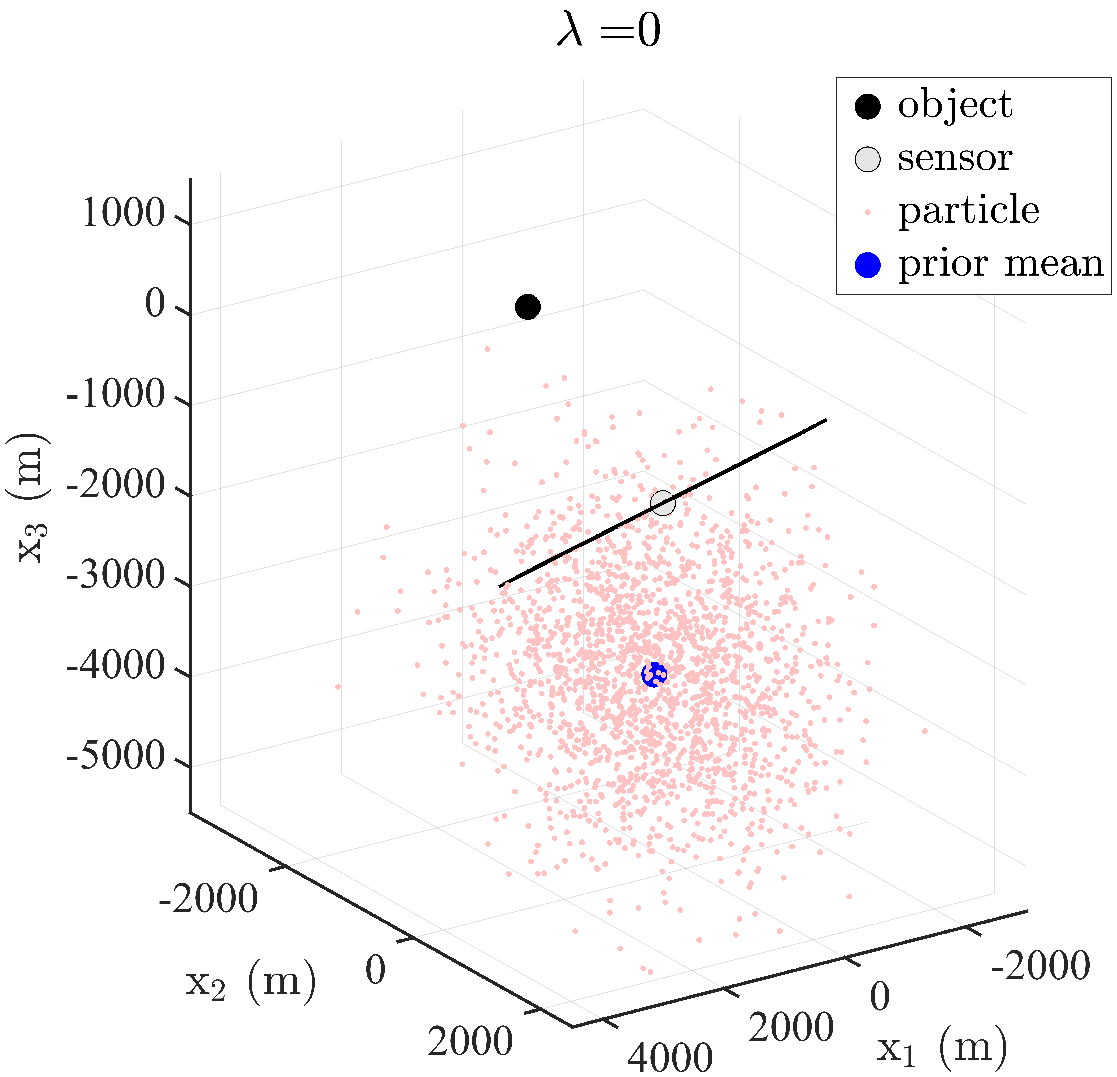
To calculate messages that, due to nonlinearities in the system model, cannot be evaluated in closed form, spa-based methods for mot typically rely on particle-based computations that closely follow the bpf (bpf) [23, 24, 25] and rely on importance sampling. A known drawback of this approach is that it typically fails in tracking problems where (i) the states of individual objects have dimensions higher than four, (ii) measurements are very informative compared to the predicted/prior pdfs. In particular, tracking of objects in 3-D Cartesian coordinates or employing sensors that yield low measurement variance often leads to a failure of particle-based computations due to particle degeneracy [26]. The particle degeneracy problem is related to the fact that predicted pdfs are used as proposal pdfs for sampling. Since predicted pdfs can have completely different shapes than the posterior pdfs, this sampling strategy is highly inefficient, i.e., few or none of the generated particles are suitable to represent the posterior pdfs. Fig. 1 shows an example of particle degeneracy in a 3-D tracking scenario with a single object and a single tdoa measurement. Particle degeneracy is exacerbated in high dimensional problems and in problems with low measurement variance. In particular, it can lead to the unwanted behavior that filter performance degrades as measurement variance is reduced. As the dimension of the problem increases, or measurement variance is reduced, the likelihood function becomes “peakier,” and it becomes more unlikely that a particle, sampled from the prior distribution, is located in a region of high likelihood.

Sometimes particle degeneracy can be avoided by using vast numbers of particles or by implementing regularization strategies [27, 25, 16]. A straightforward approach to improve sampling efficiency and avoid particle degeneracy is to design proposal pdfs that are similar to the posterior pdfs [23, 24, 25]. However, finding a distribution that is easy to sample from and simultaneously similar to posterior pdfs [23, 24, 25] is often challenging. To improve samping efficiency, adaptive importance sampling can be employed [28, 29]. In particular, auxiliary particle filters use a delayed resampling strategy to increase the number of particles with significant weights after importance sampling [30]. This approach can improve sampling efficiency but can only be applied in combination with a prediction step, which may be unavailable for newly introduced object states in MOT scenarios. Furthermore, multiple particle filtering [31], similar to a particle-based implementation of the spa, aims to increase sample efficiency by exploiting factorization of the underlying statistical model [28]. Since it relies on a suitable factorization of the conditional posterior, its applicability is restricted. Incorporating smcmc (smcmc) methods into particle filters [32, 33] is another general approach for nonlinear sequential Bayesian estimation, which is known to be very computationally expensive in high-dimensional state spaces. An alternative approach to improve sampling efficiency in sequential estimation is to perform the update step of an unscented Kalman filter [34] and use the resulting Gaussian pdf as a proposal pdf for particle filtering. The unscented particle filter [35, 36] combines this idea with a Gaussian mixture representation of predicted and posterior pdfs. To the best of our knowledge, the unscented particle filtering approach has not yet been extended to problems with mou and an unknown number of states to be

estimated.

pf [37, 38, 39, 40, 41] is a promising strategy for challenging nonlinear estimation problems that has recently received significant attention [42]. It has the potential to avoid particle degeneracy due to its ability to actively move particles representing a prior or predicted pdf to locations of high likelihood.¹¹ 1 Conventional strategies that rely on resampling also move particles but do so in a more passive way. In particular, in conventional strategies, after particles are randomly drawn, only those that correspond to locations of high likelihood remain after resampling. In challenging problems, this is prone to particle degeneracy, i.e., the number of remaining particles can become too low to be a representative description of the underlying posterior pdf.

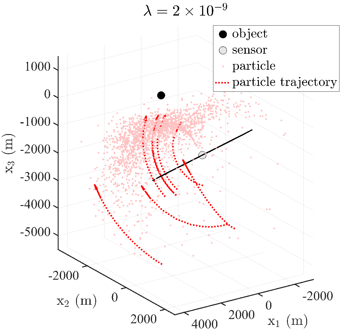
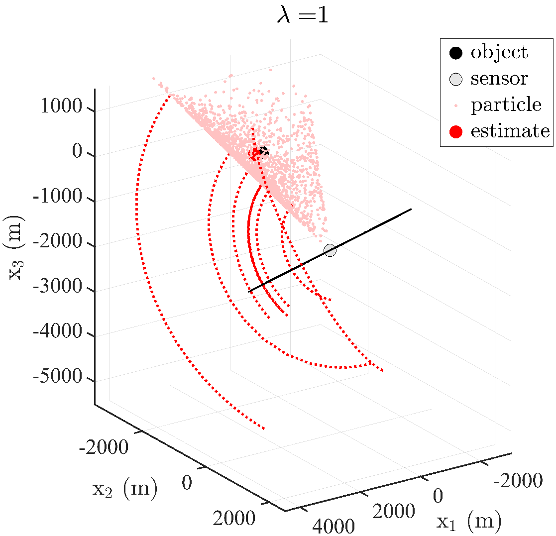
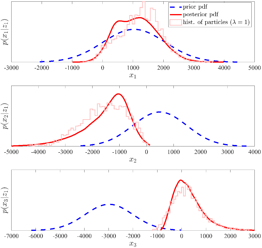
This active motion is illustrated Fig. 2. For pf a homotopy function is defined to formulate a pdf that can be smoothly deformed from the predicted pdf (or prior pdf) to the posterior pdf. pf then makes use of the homotopy function to incrementally move a set of particles sampled from the predicted pdf. In particular, a pde (pde) for particle velocity is obtained by combining the homotopy function with the Fokker-Planck equation. The particle velocity solution to the pde can be discretized and used as a transport equation for particle migration. After migration, the set of particles represents the posterior pdf. There are two different types of pf resulting in the edh (edh) filter and the ledh (ledh) filter. In the edh filter, the pf equations are computed once for the mean of all particles. In contrast, in the computationally more demanding ledh filter, the pf equations are computed for each particle individually. pf has been demonstrated to achieve a superior performance complexity tradeoff compared to existing approaches that aim at improving sampling efficiency [42]. As other particle filtering approaches, pf is highly parallelizable [38, 39, 40] and thus ideal for real-time processing on graphical processing units (GPUs).

Traditional pf methods avoid importance sampling and can only provide an approximate representation of posterior pdfs in general nonlinear systems [37, 38, 39, 40, 41]. Nevertheless, these “proposal-free” methods often lead to accurate estimation results at a significantly reduced computational complexity compared to bpf [42]. Recently, it has been shown that pf can be described by an invertible mapping and can thus be used as a measurement-driven proposal pdf for importance sampling [42]. The resulting invertible pf filter [42] is an asymptotically optimal approach to nonlinear filtering that avoids particle degeneracy and can provide accurate estimation results in high-dimensional and nonlinear problems.

A significant limitation of the pf filter presented in [42] is that it assumes that the prior or predicted pdfs follow Gaussian distributions. It is thus unsuitable for problems that involve multimodal pdfs. For problems where the measurement noise follows a Gaussian mixture pdf, [43] introduces the Gaussian sum pf filter. Here, the means of the Gaussian mixture components are updated by performing an update step similar to the ledh. On the other hand, the covariance matrices of the components are updated by extended Kalman filters that also run in parallel. An extension of [43] to the case where both driving noise and measurement noise are distributed by a Gaussian mixture pdf is presented in [44]. Here, invertible flow is used for particle weight update in an importance sampling step. For problems where both driving noise and measurement noise can be multimodal, [45] combines the invertible pf with a smcmc method that relies on the Metropolis-Hastings approach, i.e., a Metropolis-Hastings kernel is constructed using a pf algorithm based on a gmm. However, aforementioned pf approaches that can represent multimodal pdfs [43, 44, 45] are unsuitable for mot since neither model mou nor an unknown number of states to be estimated. For the cooperative localization problem, a method that relies on invertible pf is presented in [46, 47]. This method is not suitable for the more challenging multiobject tracking problems since it can only be applied to problems without measurement origin uncertainty, known number of states to be estimated, and posterior pdfs with simple, unimodal shapes. A variant of the pf filter has been proposed for mot [8]. In particular, edh and ledh variants of the single-sensor $\delta$-Generalized Labeled Multi-Bernoulli filter [7] with invertible flow are presented. These approaches are unsuitable for multiobject tracking problems where measurements are provided by multiple sensors.

We develop a method for multisensor mot with improved sample efficiency that can be used in scenarios with high-dimensional object states and informative measurements. Of particular interest are multisensor mot problems, where inexpensive sensors are used and the tracking of objects in Cartesian coordinates is impossible based on the measurements provided by a single sensor. In this type of tracking problems, the measurement of a single sensor typically has a lower dimension than the positions of objects. Consider a scenario where object positions are 3-D, but sensors only provide 1-D measurements, e.g., times of arrival (TOAs), time differences of arrival (TDOAs), or directions of arrival (DOAs). In this type of mot problem, prior or predicted pdfs can have complicated multimodal shapes, e.g., spheres, hyperboloids, or cones at the initial step after the appearance of a new object. As an example, Figs. 1 and 2 show the hyperboloid-shaped pdfs resulting from a TDOA measurement model in a 3-D tracking scenario.

Our approach performs spa-based message passing on the factor graph for scalable multisensor mot developed in [10]. The messages of the spa are computed sequentially across sensors. To improve sampling efficiency, we embed invertible particle flow into spa computations. For the evaluations of particle weights, invertible particle flow relies on a Gaussian representation of the prior or predicted pdf at the onset of the flow. To represent beliefs of object states with complicated non-Gaussian shapes, such as, e.g., hyperboloids, as in the example in Figs. 1 and 2, we make use of a gmm representation that is known to be asymptotically optimal [48]. Combining a gmm with an efficient sampling approach to represent pdfs with complicated shapes in high dimensions is inspired by unscented particle filtering [35, 36]. A general proposal pdf that takes mou into account and consists of a mixture of pdfs related to different particle flows is developed. The resulting computations are asymptotically optimal. In particular, since particles are migrated towards regions of high likelihood, an accurate approximation of spa messages with a relatively small number of particles is obtained.

The technical novelty of the proposed method lies in a new method for multitarget tracking that can achieve a superior runtime–estimation accuracy tradeoff in nonlinear and high-dimensional problems by improving sampling efficiency. The improved tradeoff is obtained by carefully embedding invertible pf. In particular, to address mou, association probabilities are computed by performing parallel flows, one for each component of the gmm and each possible measurement-to-object association. The particles of the parallel flows are weighted based on association probabilities and combined into a mixture of flows. The mixture of flows provides samples of the proposal for importance sampling. Since all flows are invertible, it is possible to evaluate the proposal pdf represented by the mixture of flows at each particle. Thus, the resulting spa-based computation of beliefs is asymptotically optimal in the sense that the resulting particle representation of the beliefs provided by the spa is arbitrarily accurate for an increasingly large number of Gaussian components and a number of particles. Our method, for the first time, performs mot with probabilistic data association based on pf.

We further demonstrate that the proposed multisensor mot can outperform reference methods based on conventional (“bootstrap”) and unscented particle filtering in a 3-D passive source tracking scenario. In particular, in the considered realistic source tracking scenario, graph-based MOT based on conventional particle filtering [9] cannot provide acceptable estimation accuracy. The also considered, yet unpublished, implementation of graph-based MOT based on unscented particle filtering, has a lower estimation accuracy but a higher runtime compared to the proposed method that embeds

invertible pf.

Key contributions of this paper are as

follows.

• •

  We develop a graph-based MOT method based on a GMM and invertible PFL for challenging scenarios with high-dimensional object states and arbitrarily shaped posterior pdfs.

• •

  We demonstrate that the proposed method can significantly outperform reference techniques in a challenging 3-D passive source multisensor mot scenario and show tracking results using real passive acoustic data.

This paper advances over the preliminary account of our method provided in the conference publication [49] by (i) introducing a gmm for multimodal state distribution with dynamic kernel resampling; (ii) considering the multisensor mot problem; (iii) presenting an improved proposal distribution based on pf; (iv) performing a comprehensive numerical evaluation in a 3-D passive source tracking scenario; and (v) applying the proposed method to an underwater acoustic dataset²² 2 More details on the application of the proposed method to the problem of tracking multiple whales underwater by performing tdoa measurements of their echolocation clicks, is presented in the companion paper [50]. Contrary to the approach presented in [8], the proposed method is suitable for multisensor scenarios. In addition, spa-based processing makes our approach scalable with respect to relevant system parameters.

Notation: Random variables are displayed in sans serif, upright fonts and their realizations in serif, italic fonts. Vectors and matrices are denoted by bold lowercase and uppercase letters, respectively. For example, a random variable and its realization are denoted by $\mathsfbr{x}$ and $x$, respectively, and a random vector and its realization by $\bm{\mathsfbr{x}}$ and $\bm{x}$, respectively. Furthermore, $\|\bm{x}\|$ and ${\bm{x}}^{\text{T}}$ denote the Euclidean norm and the transpose of vector $\bm{x}$, respectively; and $\propto$ indicates equality up to a normalization factor. ${\cal{N}}(\bm{x};\bm{x}^{\ast},\bm{P})$ denotes the Gaussian pdf (of random vector $\bm{\mathsfbr{x}}$) with mean $\bm{x}^{\ast}$ and covariance

matrix $\bm{P}$. The trace of matrix $\bm{M}$ is denoted as $\mathrm{Tr}\{\bm{M}\}$. Finally, $1(a)$ denotes the indicator function of the event $a\hskip-0.85358pt=\hskip-0.85358pt0$, i.e., $1(a)\hskip-0.85358pt=\hskip-0.85358pt1$ if $a\hskip-0.85358pt=\hskip-0.85358pt0$ and $0$

otherwise.

pf [37, 38, 39, 40] is an approach that aims at avoiding particle degeneracy. Here, particles are smoothly migrated in the state space from a representation of the prior pdf to a representation of the posterior pdf by solving a pde. Let us introduce the homotopy function $\pi_{\lambda}(\bm{x})\hskip-0.85358pt=f(\bm{x})\hskip 0.85358ptl^{\lambda}(\bm{x})$ where $\lambda\!\in\![0,1]$ is the pseudo time of the flow process and $l(\bm{x})\hskip-0.85358pt=\hskip-0.85358ptf(\bm{z}|\bm{x})$ is the likelihood function. Note that for $\lambda\hskip-0.85358pt=\hskip-0.85358pt1$, the homotopy function is equal to the unnormalized posterior pdf, i.e., $\pi(\bm{x})\triangleq\pi_{1}(\bm{x})=f(\bm{x})\hskip 0.85358ptl(\bm{x})$. The log-homotopy function is then given

by [37, 38],

The log-homotopy function is a pseudo posterior pdf in the log domain that defines a smooth and continuous deformation from $\phi(\bm{x},0)\hskip-0.85358pt=\hskip-0.85358pt\log f(\bm{x})$ to $\phi(\bm{x},1)\hskip-0.85358pt=\log\pi(\bm{x})$. This deformation describes the pf process.

It can be shown that the stochastic process defined by homotopy function $\pi_{\lambda}(\bm{x})$ satisfies the Fokker-Planck equation [41, 40, 39]. Combining the Fokker-Planck equation for the zero-diffusion case with (2) results in the following

pde [40, 39]

where $\bm{\zeta}(\bm{x},\lambda)\hskip-0.85358pt=\hskip-0.85358pt\frac{\mathrm{d}\bm{x}}{\mathrm{d}\lambda}$ describes particle velocity (samples of $\bm{\mathsfbr{x}}$) as the pseudo time $\lambda$ increases from $0$ to $1$, i.e., as the homotopy function is deformed from the prior pdf to the posterior pdf. This migration is referred to as the

pf.

If $f(\bm{x})$ and $l(\bm{x})$ are Gaussians or in another exponential family, then an exact and closed form solution for (3) is available. The edh filter [52, 39] makes use of this closed-form solution in its update step. More precisely, let $f(\bm{x})={\cal{N}}(\bm{x};\bm{x}_{0}^{\ast},\bm{P})$ and $\bm{\mathsfbr{z}}=\bm{H}\bm{\mathsfbr{x}}+\bm{\mathsfbr{v}}$ be a linear measurement model with measurement noise $\bm{\mathsfbr{v}}\sim{\cal{N}}(\bm{v};\bm{0},\bm{R})$. The exact flow solution [52, 39] now

reads $\bm{\zeta}(\bm{x},\lambda)=\bm{A}(\lambda)\bm{x}+\bm{b}(\lambda)$ where we introduce

and

Note that in (), $\bm{z}$ is the observed and thus fixed measurement.

This solution is extended to the nonlinear measurement model $\bm{\mathsfbr{z}}=\bm{h}(\bm{\mathsfbr{x}})+\bm{\mathsfbr{v}}$ by performing a suboptimal linearization step. In particular, in a first-order approximation, a Jacobian matrix is computed

, i.e. $\bm{H}(\lambda)=\left.\frac{\partial\bm{h}(\bm{x})}{\partial\bm{x}}\right|_{\bm{x}={\bm{x}}^{\ast}_{\lambda}}\hskip-0.85358pt$ where ${\bm{x}}^{\ast}_{\lambda}$ is the approximated mean of $\bm{x}$ at pseudo time $\lambda$.

In a practical implementation, we calculate $\bm{\zeta}(\bm{x},\lambda)$ at $N_{\lambda}$ discrete values of $\lambda$, i.e., $0=\lambda_{0}<\lambda_{1}<...<\lambda_{N_{\lambda}}=1$, to perform the pf. Here, we first sample $N_{\mathrm{p}}$ particles $\big\{\bm{x}_{0}^{(i)}\big\}_{i=1}^{N_{\mathrm{p}}}\!\triangleq\!\big\{\bm{x}_{\lambda_{0}}^{(i)}\}_{i=1}^{N_{\mathrm{p}}}$ from $f({\bm{x}})$. Next, at each discrete pseudo time step $l\hskip-0.85358pt\in\hskip-0.85358pt\{1,\dots,N_{\lambda}\}$, particles are migrated according to

for all $i\hskip-0.85358pt\in\hskip-0.85358pt\{1,\dots,N_{\mathrm{p}}\}$. Here, the linearized flow solution $\tilde{\bm{\zeta}}(\bm{x}^{(i)}_{\lambda_{l-1}},\lambda_{l})=\bm{A}_{l}\bm{x}^{(i)}_{\lambda_{l-1}}\hskip-0.85358pt+\hskip-0.85358pt\bm{b}_{l}$ is computed based on $\bm{A}_{l}$ and $\bm{b}_{l}$ given by (cf. (4) and ())

Note that $\bm{e}_{l}=\bm{h}({\bm{x}}^{\ast}_{\lambda_{l-1}},0)-\bm{H}_{l}{\bm{x}}^{\ast}_{\lambda_{l-1}}$ is the error of linear- ization and that the linearized measurement model, $\bm{H}_{l}$, is computed based on the mean of the last step $l-1$, i.e.,

The mean at which the measurement model is linearized is typically propagated in parallel to the particles, i.e., ${\bm{x}}^{\ast}_{\lambda_{l}}={\bm{x}}^{\ast}_{\lambda_{l-1}}+\tilde{\bm{\zeta}}({\bm{x}}^{\ast}_{\lambda_{l-1}},\lambda_{l})(\lambda_{l}-\lambda_{l-1})$.

After the last discrete pseudo time step, $l\hskip-0.85358pt=\hskip-0.85358ptN_{\lambda}$, particles $\{\bm{x}_{1}^{(i)}\}_{i=1}^{N_{\mathrm{p}}}\!\triangleq\!\{\bm{x}_{\lambda_{N_{\lambda}}}^{(i)}\}_{i=1}^{N_{\mathrm{p}}}$ that approximately represent the unnormalized posterior pdf $\pi(\bm{x})$ are finally obtained. Pseudocode for the pf update step is provided in Algorithm 1. pf based on a linearized model has no optimality guarantees. However, it has been demonstrated numerically to typically provide an accurate representation of the posterior pdf $f(\bm{x}|\bm{z})$[37, 38, 39, 40, 41, 42]. In what follows, the pf related to the measurement $\bm{z}$ as defined by (6)–(8), is denoted as $\bm{\mathsfbr{x}}_{0}\hskip-0.85358pt\xrightarrow{\hskip-0.85358pt}\bm{z}\hskip-0.85358pt\xrightarrow{\hskip-0.85358pt}\bm{\mathsfbr{x}}_{1}$ or for notational convenience in future derivations as

$\bm{\mathsfbr{x}}_{0}\hskip-0.85358pt\xrightarrow{\hskip-0.85358pt}\bm{z}\hskip-0.85358pt\xrightarrow{\hskip-0.85358pt}\bm{\mathsfbr{x}}$.

As an alternative to edh pf as discussed above, ledh pf has been introduced in [53, 42]. Here, a linearization is performed for each particle location individually instead of only at the mean particle location, i.e., individual flow parameters $\bm{H}_{l}^{(i)},\bm{A}_{l}^{(i)}$, and $\bm{b}_{l}^{(i)}$ are computed to migrate the particles along their individual flows. Although the ledh flow usually outperforms the edh flow, it suffers from considerable computational complexity since the main computational burden is related to calculating the flow parameters.

In Fig. 2, it is depicted how pf actively move particles representing a prior or predicted pdfs to locations of high likelihood. Active motion of particles leads to a significantly improved approximation of the posterior pdf compared to conventional importance sampling shown in

Fig. 1.

pf can be used to compute a measurement-driven proposal pdf $q(\bm{x}|\bm{z})$ for importance sampling (cf. (1)) to perform asymptotically optimal estimation [42]. Here, the mapping as performed by pf $\bm{\mathsfbr{x}}_{0}\hskip-0.85358pt\xrightarrow{\hskip-0.85358pt}\bm{z}\hskip-0.85358pt\xrightarrow{\hskip-0.85358pt}\bm{\mathsfbr{x}}\hskip-0.85358pt\hskip-0.85358pt$ is invertible, i.e., there exists an invertible mapping of the particles after the flow $\big\{\bm{x}^{(i)}\big\}_{i=1}^{N_{\mathrm{p}}}$ to the particles $\big\{\bm{x}_{0}^{(i)}\big\}_{i=1}^{N_{\mathrm{p}}}$ if certain constraints on the differences of consecutive discrete pseudo times $\lambda_{l}-\lambda_{l-1}$, $l\hskip-0.85358pt\in\hskip-0.85358pt\{1,\dots,N_{\lambda}\}$ are satisfied [42].

By exploiting the invertible mapping, the proposal pdf resulting from pf can be evaluated at the particles

as [42]

Here, the “mapping factor” $\theta$ is defined

as

By plugging (10) into (1) the weight of the particle $\bm{x}^{(i)}$ is obtained

as

The resulting particle set $\{\bm{x}^{(i)},w^{(i)}\}_{i=1}^{N_{\mathrm{p}}}$ is an asymptotically optimal sample representation of the posterior pdf $f(\bm{x}|\bm{z})$ that can often provide accurate estimation results in nonlinear and high-dimensional estimation problems even if the number of particles is moderate [42]. Pseudocode for importance sampling with invertible pf is provided in Algorithm 2. Note that since the pf used for the measurement-driven proposal pdf is typically based on the edh filter update step, a Gaussian prior pdf is

assumed.

An approximate Gaussian representation of this posterior distribution can be subsequently obtained by applying Algorithm 3 which calculates a mean ${\bm{x}}^{\ast}_{1}$ and a covariance matrix $\bm{P}_{1}$ from the unnormalized weighted particles $\big\{{\bm{x}}^{(i)}_{1}\hskip-0.85358pt,w_{1}^{(i)}\big\}_{i=1}^{N_{\mathrm{p}}}$. Note that in Algorithm 2, the same mapping factor $\theta$ is used to calculate all particle weights. If Algorithm 3 is applied after Algorithm 2, this factor is irrelevant since all weights are normalized in Algorithm 3. However, making use of $\theta$ is important if multiple flows are performed in parallel, as will be discussed in

Section III.

Note that instead of a particle-based covariance matrix computation as performed in Line 7 of Algorithm 3, an extended or unscented Kalman update step can be used [42]. For a large number of particles $N_{\mathrm{p}}$, a particle-based computation is more accurate than a computation based on the extended or unscented Kalman update

step.

As discussed in the previous Section II, for the evaluations of particle weights, invertible particle flow relies on a Gaussian representation of the prior pdf at the onset of the flow. In challenging multisensor MOT problems, the complicated multimodal shapes of prior and posterior pdfs (see, e.g., the hyperboloid-shaped posterior pdf in Fig. 2) can often not be approximated accurately by a single Gaussian. A gmm aims at representing multimodal distributions based on an additively weighted combination of multiple Gaussian components. Each Gaussian component is typically referred to as a “kernel”. Let $N_{\mathrm{k}}$ be the total number of kernels and let $h\in\{1,\dots,N_{\mathrm{k}}\}$ be the kernel index. A multimodal prior pdf that follows a gmm representation can then be written as $f(\bm{x})=\frac{1}{N_{\mathrm{k}}}\sum_{h=1}^{N_{\mathrm{k}}}{\cal{N}}\big(\bm{x};\bm{x}^{\ast(h)},\bm{P}^{(h)}\big)$. The corresponding multimodal posterior pdf $f(\bm{x}|\bm{z})$ can be computed by performing Algorithm 2 and Algorithm 3 $N_{\mathrm{k}}$ times in parallel, i.e., one instance of both algorithms is performed for each kernel ${\cal{N}}\big(\bm{x};\bm{x}^{\ast(h)},\bm{P}^{(h)}\big)$, $h\hskip-0.85358pt\in\hskip-0.85358pt\{1,\dots,N_{\mathrm{k}}\}$. To obtain a gmm representation composed of an arbitrary number $N^{\prime}_{\mathrm{k}}$ of kernels, a resampling step is then performed, i.e., $N^{\prime}_{\mathrm{k}}$ particles are drawn from the overall $N_{\mathrm{k}}N_{\mathrm{p}}$ particles based on their weights $w_{1}^{(h,i)}\hskip-0.85358pt$. The resampled particles represent the mean of $N^{\prime}_{\mathrm{k}}$ new kernels. The covariance of the new kernels is inherited from the original kernel the mean was sampled from. Pseudocode for gmm importance sampling with invertible pf is provided in Algorithm 4. Importance sampling with invertible pf makes use of resampling as presented in

Algorithm 5.

For $N_{\mathrm{k}}=1$ and $N_{\mathrm{p}}>1$, this importance sampling approach is equivalent to invertible pf based on the edh update step. Furthermore, if $N_{\mathrm{p}}=1$, $N_{\mathrm{k}}>1$, this importance sampling approach is equivalent to invertible pf based on the ledh update step. Note that for $N_{\mathrm{p}}\hskip-0.85358pt=\hskip-0.85358pt1$, as performed by the ledh, an additional extended or unscented Kalman update step needs to be used to calculate an approximate covariance matrix

[42].

In a variety of estimation problems, the measurement model suffers from a deficiency beyond measurement noise referred to as mou [3]. Here, there is a single object but multiple measurements and it is not known which measurement was generated by the object. Consider a single object with state $\bm{\mathsfbr{x}}$ and measurements $\bm{\mathsfbr{z}}^{(m)}\hskip-0.85358pt$, $m\hskip-0.85358pt\in\{1,\dots,M\}$. If $m^{\prime}$ is the measurement that was generated by the object, the corresponding measurement model is given by $\bm{\mathsfbr{z}}^{(m^{\prime})}=\bm{h}(\bm{\mathsfbr{x}})+\bm{\mathsfbr{v}}$. Based on this model, the conditional pdf of the object-originated measurement $\bm{z}^{(m^{\prime})}$ reads $f_{\hskip-0.85358pt\mathrm{o}\hskip-0.85358pt}\big(\bm{z}^{(m^{\prime})}|\bm{x}\big)$. All the other measurements are fps that follow the fp pdf $f_{\mathrm{fp}\hskip-0.85358pt}\big(\bm{z}^{(m^{\prime})}\big)$. It is assumed that at most one measurement originates from the object. The probability that the object generates a measurement is $p_{\mathrm{d}}$, and the mean number of fps is Poisson distributed with mean $\mu_{\mathrm{fp}}$. Since it is unknown which measurement was generated by the object, a discrete and random association variable $\mathsfbr{a}\in\{0,1,\dots,M\}$ is introduced. Here, $\mathsfbr{a}\hskip-0.85358pt=\hskip-0.85358pt0$ describes the event where no measurement originated from the object and $\mathsfbr{a}\hskip-0.85358pt=\hskip-0.85358ptm$, $m\hskip-0.85358pt\in\{1,\dots,M\}$ describes the event where measurement $\bm{\mathsfbr{z}}^{(m)}$ was originated from the object. Let $\bm{\mathsfbr{z}}=[\bm{\mathsfbr{z}}^{(1)\mathrm{T}},\dots,\bm{\mathsfbr{z}}^{(M)\mathrm{T}}]^{\mathrm{T}}$ be the joint measurement vector. Following common assumptions [3], conditioned on $\bm{\mathsfbr{x}}$, the joint pdf of $\bm{\mathsfbr{z}}$ and $\mathsfbr{a}$ is given

by

For $\bm{z}$ fixed, one can use this conditional pdf to directly compute the mou likelihood function

and the marginal

pmf (pmf)

The values of the pmf $p(a|\bm{z})$ are also referred to as marginal association probabilities [3], i.e., they represent the probability of a particular association event $a\hskip-0.85358pt\in\hskip-0.85358pt\{0,\dots,M\}$ conditioned on an observed

$\bm{z}$.

In principle, the mou likelihood function in (14) can be directly used for importance sampling as in (1). However, in problems with mou, importance sampling based on invertible pf is complicated by the fact that there are multiple measurements, and it is thus not clear which measurement should be used to compute pf parameters (7) and (8), i.e., the pf proposal pdf $q_{\mathrm{PFL}}(\bm{x}_{1}^{{(i)}}|\bm{z})$ in (10) cannot be directly used. To address this problem, we propose the combined

proposal pdf

where we used the marginal association probabilities $p(a|\bm{z})$ to weight the proposal pdfs $q_{\mathrm{PFL}}\big(\bm{x}|\bm{z}^{(m)}\big)$ related to pf based on measurements $\bm{z}^{(m)}\hskip-0.85358pt$, $m\hskip-0.85358pt\in\hskip-0.85358pt\{1,\dots,M\}$ (cf. (10)) and the Gaussian prior pdf $f(\bm{x})={\cal{N}}(\bm{x};\bm{x}_{0}^{\ast},\bm{P})$. In particular, recall that the proposal

distribution $q_{\mathrm{PFL}}\big(\bm{x}|\bm{z}^{(m)})$ related to the pf $\bm{\mathsfbr{x}}_{0}\hskip-0.85358pt\xrightarrow{\hskip-0.85358pt}\bm{z}^{(m)}\hskip-0.85358pt\xrightarrow{\hskip-0.85358pt}\bm{\mathsfbr{x}}^{(m)}$, can be evaluated

as

where $\theta^{(m)}$ is the mapping factor.

A total of $(M+1)N_{\mathrm{p}}$ particles representing the proposal pdf in (16) is obtained by drawing $N_{\mathrm{p}}$ particles for each of the $M+1$ components in (16) and calculating corresponding marginal association probabilities and weights. For the first component related to association event $\mathsfbr{a}\hskip-0.85358pt=\hskip-0.85358pt0$, $N_{\mathrm{p}}$ particles $\big\{\bm{x}^{(i,0)}\big\}^{N_{\mathrm{p}}}_{i=1}$ are directly drawn from $f(\bm{x})$, the corresponding marginal association probability is obtained by using (13) in (15), i.e., $p(a\hskip-0.85358pt=\hskip-0.85358pt0|\bm{z})\hskip-0.85358pt\propto\hskip-0.85358pt1-p_{\mathrm{d}}$, and the corresponding combined proposal weights are set to $\omega^{\prime(i,0)}\hskip-0.85358pt=\hskip-0.85358ptp(a\hskip-0.85358pt=\hskip-0.85358pt0|\bm{z})\hskip 0.85358pt\hskip 0.85358pt{\cal{N}}(\bm{x}_{0}^{(i,0)};\bm{x}_{0}^{\ast},\bm{P})$ (cf. (16)). For each other component related to association event $\mathsfbr{a}\hskip-0.85358pt=\hskip-0.85358ptm$, $m\hskip-0.85358pt\in\hskip-0.85358pt\{1,\dots,M\}$, first $N_{\mathrm{p}}$ particles

$\big\{\bm{x}^{(i,m)}_{0}\big\}^{N_{\mathrm{p}}}_{i=1}$ are drawn from $f(\bm{x})$. Next, the pf $\bm{\mathsfbr{x}}_{0}\hskip-0.85358pt\xrightarrow{\hskip-0.85358pt}\hskip-0.85358pt\hskip-0.85358pt\hskip-0.85358pt\bm{\mathsfbr{z}}^{(m)}\hskip-0.85358pt\hskip-0.85358pt\xrightarrow{\hskip-0.85358pt}\hskip-0.85358pt\bm{\mathsfbr{x}}^{(m)}$ is applied

to

the particles $\big\{\bm{x}^{(i,m)}_{0}\big\}^{N_{\mathrm{p}}}_{i=1}$ and new particles $\big\{\bm{x}^{(i,m)}\big\}^{N_{\mathrm{p}}}_{i=1}$ are obtained for each $m\hskip-0.85358pt\in\hskip-0.85358pt\{1,\dots,M\}$. An approximation of each marginal association probability $\tilde{p}(a=m|\bm{z})$, $m\hskip-0.85358pt\in\hskip-0.85358pt\{1,\dots,M\}$ is finally calculated from these particles by using (13) in (15) and performing Monte Carlo integration [24] based on the proposal pdf $q_{\mathrm{PFL}}\big(\bm{x}^{{(i,m)}}|\bm{z}^{(i,m)}\big)$ in (17),

i.e.,

The

corresponding combined proposal

weights are

set according

to (cf. (16) and

(17))

Finally, we reindex the resulting particles and

weights $\big\{\big(\hskip 0.85358pt\omega^{\prime(i,a)}\hskip-0.85358pt\hskip-0.85358pt,$ $\bm{x}^{(i,a)}\big)\big\}^{N_{\mathrm{p}}}_{i=1}$, $a\hskip-0.85358pt\in\hskip-0.85358pt\{0,\dots,M\}$ to

obtain $\big\{\big(\hskip 0.85358pt\omega^{(l)},$ $\bm{x}^{(l)}\big)\big\}^{L}_{l=1}$ where $l=i(a+1)$ and $L=N_{\mathrm{p}}\hskip 0.85358pt(M+1)$.

Following the importance sampling principle

, we next aim to compute particles $\big\{\big(\hskip 0.85358ptw^{(\hskip 0.56905ptl)}\hskip-0.85358pt\hskip-0.85358pt,\bm{x}^{(\hskip 0.56905ptl)}\big)\big\}^{L}_{l=1}$ that represent the posterior pdf $f(\bm{x}|\bm{z})$. In particular, by

plugging (14) into (1) and by using $\big\{\big(\hskip 0.85358pt\omega^{(l)}\hskip-0.85358pt\hskip-0.85358pt,\bm{x}^{(l)}\big)\big\}$ (cf. (19)) to represent $q(\bm{x}|\bm{z})$ in (1), we

obtain

The resulting set of particles $\big\{\big(\hskip 0.85358ptw^{(\hskip 0.56905ptl)}\hskip-0.85358pt\hskip-0.85358pt,\bm{x}^{(\hskip 0.56905ptl)}\big)\big\}^{L}_{l=1}$ is an asymptotically optimal representation of $f(\bm{x}|\bm{z})$ for scenarios with

mou.

For problems where the prior distribution is non-Gaussian and potentially multimodal, gmm pf with invertible flow discussed in Section III-A can be directly applied to problems with mou. Pseudocode for gmm importance sampling with the invertible flow for mou problems is provided in Algorithm 6. Algorithm 6 relies on the measurement evaluation presented in Algorithm 7 and the measurement update presented in Algorithm 8. Note that in Algorithm 8, for future reference, we have also introduced extrinsic data association information denoted as $\kappa^{(a)}$, $a\in\{0,\dots,M\}$. In the single object tracking considered here, we have $\kappa^{(a)}=1$.

References

- [1] M. Zimmer, S. Dolman, and L. Weilgart, Passive acoustic monitoring of cetaceans. Cambridge, UK: Cambridge Univ. Press, 2011.
- [2] K. L. Cummins and M. J. Murphy, “An overview of lightning locating systems: History, techniques, and data uses, with an in-depth look at the U.S. NLDN,” IEEE Trans. Electromagn. Compat., vol. 51, no. 3, pp. 499–518, 2009.
- [3] Y. Bar-Shalom, P. K. Willett, and X. Tian, Tracking and Data Fusion: A Handbook of Algorithms. Storrs, CT: Yaakov Bar-Shalom, 2011.
- [4] D. B. Reid, “An algorithm for tracking multiple targets,” IEEE Trans. Autom. Control, vol. 24, no. 6, pp. 843–854, Dec. 1979.
- [5] R. Mahler, Statistical Multisource-Multitarget Information Fusion. Norwood, MA: Artech House, 2007.
- [6] J. L. Williams, “Marginal multi-Bernoulli filters: RFS derivation of MHT, JIPDA and association-based MeMBer,” IEEE Trans. Aerosp. Electron. Syst., vol. 51, no. 3, pp. 1664–1687, Jul. 2015.
- [7] B.-N. Vo, B.-T. Vo, and H. G. Hoang, “An efficient implementation of the generalized labeled multi-Bernoulli filter,” IEEE Trans. Signal Process., vol. 65, no. 8, pp. 1975–1987, 2017.
- [8] A. Saucan, Y. Li, and M. Coates, “Particle flow SMC delta-GLMB filter,” in Proc. IEEE ICASSP-17, New Orleans, LA, USA, Mar. 2017, pp. 4381–4385.
- [9] F. Meyer, P. Braca, P. Willett, and F. Hlawatsch, “A scalable algorithm for tracking an unknown number of targets using multiple sensors,” IEEE Trans. Signal Process., vol. 65, no. 13, pp. 3478–3493, Jul. 2017.
- [10] F. Meyer, T. Kropfreiter, J. L. Williams, R. A. Lau, F. Hlawatsch, P. Braca, and M. Z. Win, “Message passing algorithms for scalable multitarget tracking,” Proc. IEEE, vol. 106, no. 2, pp. 221–259, Feb. 2018.
- [11] G. Soldi, F. Meyer, P. Braca, and F. Hlawatsch, “Self-tuning algorithms for multisensor-multitarget tracking using belief propagation,” IEEE Trans. Signal Process., vol. 67, no. 15, pp. 3922–3937, Aug. 2019.
- [12] A. Tesei, F. Meyer, and R. Been, “Tracking of multiple surface vessels based on passive acoustic underwater arrays,” J. Acoust. Soc. Am., vol. 147, no. 2, pp. EL87–EL92, 2020.
- [13] F. Meyer and J. L. Williams, “Scalable detection and tracking of geometric extended objects,” IEEE Trans. Signal Process., vol. 69, pp. 6283–6298, 2021.
- [14] F. R. Kschischang, B. J. Frey, and H.-A. Loeliger, “Factor graphs and the sum-product algorithm,” IEEE Trans. Inf. Theory, vol. 47, no. 2, pp. 498–519, Feb. 2001.
- [15] H. Wymeersch, J. Lien, and M. Z. Win, “Cooperative localization in wireless networks,” Proc. IEEE, vol. 97, no. 2, pp. 427–450, 2009.
- [16] F. Meyer, O. Hlinka, H. Wymeersch, E. Riegler, and F. Hlawatsch, “Distributed localization and tracking of mobile networks including noncooperative objects,” IEEE Trans. Signal Inf. Process. Netw., vol. 2, no. 1, pp. 57–71, Mar. 2016.
- [17] M. Z. Win, F. Meyer, Z. Liu, W. Dai, S. Bartoletti, and A. Conti, “Efficient multisensor localization for the internet of things: Exploring a new class of scalable localization algorithms,” IEEE Signal Process. Mag., vol. 35, no. 5, pp. 153–167, 2018.
- [18] B. Teague, Z. Liu, F. Meyer, A. Conti, and M. Z. Win, “Network localization and navigation with scalable inference and efficient operation,” IEEE Trans. Mobile Comput., vol. 21, no. 6, pp. 2072–2087, 2022.
- [19] E. Leitinger, F. Meyer, F. Hlawatsch, K. Witrisal, F. Tufvesson, and M. Z. Win, “A belief propagation algorithm for multipath-based SLAM,” IEEE Trans. Wireless Commun., vol. 18, no. 12, pp. 5613–5629, 2019.
- [20] X. Li, E. Leitinger, A. Venus, and F. Tufvesson, “Sequential detection and estimation of multipath channel parameters using belief propagation,” IEEE Trans. Wireless Commun., vol. 21, no. 10, pp. 8385–8402, 2022.
- [21] E. Leitinger, A. Venus, B. Teague, and F. Meyer, “Data Fusion for Multipath-Based SLAM: Combing Information from Multiple Propagation Paths,” 2022, available online: https://arxiv.org/abs/2211.09241.
- [22] F. Meyer and K. L. Gemba, “Probabilistic focalization for shallow water localization,” J. Acoust. Soc, vol. 150, no. 2, pp. 1057–1066, 2021.
- [23] N. J. Gordon, D. J. Salmond, and A. F. M. Smith, “Novel approach to nonlinear/non-Gaussian Bayesian state estimation,” IEE Proc. F, vol. 140, no. 2, pp. 107–113, 1993.
- [24] A. Doucet, N. de Freitas, and N. Gordon, Sequential Monte Carlo Methods in Practice. Springer, 2001.
- [25] M. S. Arulampalam, S. Maskell, N. Gordon, and T. Clapp, “A tutorial on particle filters for online nonlinear/non-Gaussian Bayesian tracking,” IEEE Trans. Signal Process., vol. 50, no. 2, pp. 174–188, Feb. 2002.
- [26] P. Bickel, B. Li, and T. Bengtsson, “Sharp failure rates for the bootstrap particle filter in high dimensions,” in Pushing the Limits of Contemporary Statistics: Contributions in Honor of Jayanta K. Ghosh, vol. 3. Beachwood, OH, USA: Inst. Math. Statist., 2008, pp. 318–329.
- [27] C. Musso, N. Oudjane, and F. Le Gland, “Improving regularised particle filters,” in Sequential Monte Carlo Methods in Practice. Springer, New York, NY, 2001, pp. 247–271.
- [28] M. F. Bugallo, V. Elvira, L. Martino, D. Luengo, J. Miguez, and P. M. Djuric, “Adaptive importance sampling: The past, the present, and the future,” IEEE Signal Process. Mag., vol. 34, no. 4, pp. 60–79, 2017.
- [29] V. Elvira, L. Martino, M. F. Bugallo, and P. M. Djuric, “Elucidating the auxiliary particle filter via multiple importance sampling [lecture notes],” IEEE Signal Process. Mag., vol. 36, no. 6, pp. 145–152, 2019.
- [30] M. K. Pitt and N. Shephard, “Filtering via simulation: Auxiliary particle filters,” J. Am. Statist. Assoc., vol. 94, no. 446, pp. 590–599, Jun. 1999.
- [31] P. M. Djuric, T. Lu, and M. F. Bugallo, “Multiple particle filtering,” in Proc. ICASSP-07, vol. 3, 2007, pp. 1181–1184.
- [32] C. Berzuini, N. G. Best, W. R. Gilks, and C. Larizza, “Dynamic conditional independence models and Markov chain Monte Carlo methods,” Journal of the American Statistical Association, vol. 92, no. 440, pp. 1403–1412, 1997.
- [33] W. R. Gilks and C. Berzuini, “Following a moving target-Monte Carlo inference for dynamic Bayesian models,” J. R. Stat. Soc. Series B Stat. Methodol., vol. 63, no. 1, pp. 127–146, 2001.
- [34] S. J. Julier and J. K. Uhlmann, “Unscented filtering and nonlinear estimation,” Proc. IEEE, vol. 92, no. 3, pp. 401–422, Mar. 2004.
- [35] R. van der Merwe, A. Doucet, N. de Freitas, and E. Wan, “The unscented particle filter,” in Proc. NIPS-00, Dec. 2000, pp. 584–590.
- [36] R. van der Merwe, A. Doucet, N. de Freitas, and E. Wang, “Four hydrophone array for acoustic three-dimensional location,” Cambridge University Engineering Department, Tech. Rep. CUED/F-INFENG/TR 380, Aug. 2000.
- [37] F. Daum and J. Huang, “Nonlinear filters with log-homotopy,” in Proc. SPIE-07, Aug. 2007, pp. 423–437.
- [38] ——, “Nonlinear filters with particle flow induced by log-homotopy,” in Proc. SPIE-09, May 2009, pp. 76–87.
- [39] F. Daum, J. Huang, and A. Noushin, “Exact particle flow for nonlinear filters,” in Proc. SPIE-10, Apr. 2010, pp. 92–110.
- [40] F. Daum and J. Huang, “Particle flow with non-zero diffusion for nonlinear filters,” in Proc. SPIE-13, May 2013, pp. 226–238.
- [41] P. Bunch and S. Godsill, “Approximations of the optimal importance density using Gaussian particle flow importance sampling,” J. Amer. Statist. Assoc., vol. 111, no. 514, pp. 748–762, Aug. 2016.
- [42] Y. Li and M. Coates, “Particle filtering with invertible particle flow,” IEEE Trans. Signal Process., vol. 65, no. 15, pp. 4102–4116, Aug. 2017.
- [43] S. Pal and M. Coates, “Gaussian sum particle flow filter,” in Proc. IEEE CAMSAP-18, Curaçao, Dutch Antilles, Dec. 2017.
- [44] ——, “Particle flow particle filter for Gaussian mixture noise models,” in Proc. IEEE ICASSP-18, Calgary, Canada, 2018, pp. 4249–4253.
- [45] Y. Li, S. Pal, and M. J. Coates, “Invertible particle-flow-based sequential MCMC with extension to Gaussian mixture noise models,” IEEE Trans. Signal Process., vol. 67, no. 9, pp. 2499–2512, 2019.
- [46] L. Wielandner, E. Leitinger, F. Meyer, and K. Witrisal, “Message passing-based 9-D cooperative localization and navigation with embedded particle flow,” IEEE Trans. Signal Inf. Process. Netw., vol. 9, pp. 95–109, 2023.
- [47] L. Wielandner, E. Leitinger, F. Meyer, B. Teague, and K. Witrisal, “Message passing-based cooperative localization with embedded particle flow,” in Proc. IEEE ICASSP-22, 2022, pp. 5652–5656.
- [48] B. W. Silverman, Density Estimation for Statistics and Data Analysis. Chapman & Hall, 1986.
- [49] W. Zhang and F. Meyer, “Graph-based multiobject tracking with embedded particle flow,” in Proc. IEEE RadarConf-21, Atlanta, GA, USA, May 2021.
- [50] J. Jang, F. Meyer, E. R. Snyder, S. M. Wiggins, S. Baumann-Pickering, and J. A. Hildebrand, “Bayesian detection and tracking of odontocetes in 3-D from their echolocation clicks,” J. Acoust. Soc, vol. 153, no. 5, pp. 2690–2705, 05 2023.
- [51] Y. Bar-Shalom, T. Kirubarajan, and X.-R. Li, Estimation with Applications to Tracking and Navigation. New York, NY: Wiley, 2002.
- [52] F. Daum and J. Huang, “Exact particle flow for nonlinear filters: Seventeen dubious solutions to a first order linear underdetermined PDE,” in Proc. Asilomar-10, Pacific Grove, CA, USA, Nov. 2010, pp. 64–71.
- [53] T. Ding and M. J. Coates, “Implementation of the Daum-Huang exact-flow particle filter,” in Proc. IEEE SSP-12, Ann Arbor, MI, USA, 2012, pp. 257–260.
- [54] B. Silverman, Density Estimation for Statistics and Data Analysis. Taylor & Francis, 1986.
- [55] G. J. McLachlan, S. X. Lee, and S. I. Rathnayake, “Finite mixture models,” Annu. Rev. Stat. Appl., vol. 6, no. 1, pp. 355–378, 2019.
- [56] W. H. Press, S. A. Teukolsky, W. T. Vetterling, and B. P. Flannery, Numerical Recipes: The Art of Scientific Computing. USA: Cambridge University Press, 2007.
- [57] W. Zhang and F. Meyer, “Multisensor multiobject tracking with high-dimensional object states: Supplementary material,” 2023, https://fmeyer.ucsd.edu/ZhaMey-2023-SM.pdf.
- [58] H. V. Poor, An Introduction to Signal Detection and Estimation, 2nd ed. New York: Springer-Verlag, 1994.
- [59] J. L. Williams and R. Lau, “Approximate evaluation of marginal association probabilities with belief propagation,” IEEE Trans. Aerosp. Electron. Syst., vol. 50, no. 4, pp. 2942–2959, Oct. 2014.
- [60] Y. Bar-Shalom, X. R. Li, and T. Kirubarajan, Estimation with Applications to Tracking and Navigation. New York, NY: Wiley, 2001.
- [61] S. M. Wiggins and J. A. Hildebrand, “High-frequency acoustic recording package (HARP) for broad-band, long-term marine mammal monitoring,” in Proc. UT-07, Apr. 2007, pp. 551–557.
- [62] D. Schuhmacher, B.-T. Vo, and B.-N. Vo, “A consistent metric for performance evaluation of multi-object filters,” IEEE Trans. Signal Process., vol. 56, no. 8, pp. 3447–3457, Aug. 2008.
- [63] S. M. Wiggins and J. A. Hildebrand, “High-frequency acoustic recording package (HARP) for broad-band, long-term marine mammal monitoring,” in Proc. IEEE Int. Symp. Underw. Technol., 2007, pp. 551–557.
- [64] G. Ferri, A. Munafò, A. Tesei, P. Braca, F. Meyer, K. Pelekanakis, R. Petroccia, J. Alves, C. Strode, and K. LePage, “Cooperative robotic networks for underwater surveillance: an overview,” IET Radar Sonar Navig., vol. 11, no. 12, pp. 1740–1761, Dec. 2017.
- [65] L. Dai and F. Daum, “Stiffness mitigation in stochastic particle flow filters,” IEEE Trans. Aerosp. Electron. Syst., vol. 58, no. 4, pp. 3563–3577, 2022.
- [66] ——, “On the design of stochastic particle flow filters,” IEEE Trans. Aerosp. Electron. Syst., 2022.
- [67] F. Meyer and M. Z. Win, “Scalable data association for extended object tracking,” IEEE Trans. Signal Inf. Process. Netw., vol. 6, pp. 491–507, 2020.
- [68] F. Meyer, H. Wymeersch, M. Fröhle, and F. Hlawatsch, “Distributed estimation with information-seeking control in agent networks,” IEEE J. Sel. Areas Commun., vol. 33, no. 11, Nov. 2015.