Estimating Latent Population Flows from Aggregated Data via Inversing Multi-Marginal Optimal Transport

This work focuses on the problems where data about individuals are not readily available because of various reasons such as privacy issues and measurement fidelity. Instead, we only have access to the population-level aggregate data that could be incomplete and noisy. For instance, when studying the infectious disease spreading [5], it is too expensive or even impossible to track the trajectory of each individual. Nevertheless, the number of individuals in some regions over discrete time points, can be measured using sensing devices. Statistical analysis of these aggregate data is challenging, and has received amounts of attention in diverse fields including estimating ensemble flows [8, 15], steering opinion dynamics among humans [28], epidemic forecasting [20] among others.

Over last decade, many efforts, such as collective graphical models (CGMs) [21, 22, 25, 14], have been dedicated to the problem of inference and learning with aggregated data. These methods often assume that the individuals behind aggregated data, behave according to a time-homogeneous Markov chain. However, in many cases, the individual movement behaviors are significantly affected by various factors including weather conditions, traffic situations, and so on. Hence, estimating latent transition flows only with a time-homogeneous Markov model, may lead to a poor approximation in many cases. Recent studies [8, 9, 23] have shown that the inference (filtering) with population-level aggregated observations, is equivalent to an entropy regularized structured multi-marginal optimal transport (SMOT) problem. In particular, the SMOT framework enables us to readily apply Sinkhorn algorithm to perform efficient marginal inference in collective hidden Markov models with guaranteed convergence. Following this success, Singh et al. 2020b developed an approximate expectation-maximization (EM) algorithm to learn the transition parameter of a time-homogeneous hidden Markov process from the aggregated observations of population flows. Despite being simple and tractable, this new method still strictly assumes that each individual follows the time-homogeneous Markov chain, which thus may lead to a poor estimation of the true transition flows in real-world data.

In this work, we propose to estimate the latent transition flows from aggregated data by learning the cost functions of the structured multi-marginal optimal transport framework. By doing so, our method allows the estimated transition parameters to be time-varying, and thus demonstrated improved accuracy in analyzing real-world population flows, compared with time-homogeneous Markov models. In particular, the main contributions of this paper are:

• •

  We propose an expectation-maximization (EM)-type algorithm to simultaneously learn the cost functions of the formulated SMOT problem, and to estimate the transition flows using Sinkhorn belief propagation algorithm (Sec.4). The uniqueness of the recovered cost functions can be ensured under some mild conditions, as proved by the recent studies in inverse optimal transport [16].

• •

  We also investigate regularized convex optimization algorithms [4] to construct cost functions as sparse linear combinations of some basis distance functions, which allow to learn more complicated cost functions than symmetric ones.

• •

  Experiments are conducted on both simulated and real flow data, to demonstrate the improved performance of the proposed methods in estimating latent transition flows, compared with previous related methods.

Collective graphical models (CGMs) is proposed by [21] as a formalism to perform inference in aggregate noisy data including ensemble flows. Sheldon et al. 2013 studied the intractability of the exact marginal inference in CGMs, and proposed an approximate maximum a posteriori (MAP) estimation as a substitute. Following this success, Sun et al. 2015 developed the non-linear belief propagation algorithm to perform approximate MAP inference in CGMs. Bethe-RDA is another algorithm dedicated to aggregate inference in CGMs via regularized dual averaging (RDA) with guaranteed convergence. Recently, Bernstein and Sheldon 2016 developed an approach of moments estimator to learn the parameters of the Markov model from aggregate noisy flows. Haasler et al. 2021c, Haasler et al. 2019 recently investigated the problems of estimating ensemble flows from a graphically structured multi-marginal optimal transport perspective. In particular, Haasler et al. 2021a studied a tree-structured multi-marginal optimal transport, which allows to consider various related problems such as information fusion under a unified MOT framework. Singh et al. 2020a first studied the inference (filtering) problems in CGMs based upon the tree-structured MOT framework. Singh et al. 2020b derived an approximate EM algorithm to conduct learning and inference in time-homogeneous collective hidden Markov models.

To the best of our knowledge, most of the collective graphical models assume the observed flow data are generated by time-homogeneous Markov models. In contrast, we aim to learn the time-dependent transition matrices indirectly by learning the corresponding cost functions. Our methods are based upon graphical-structured multi-marginal optimal transport (MOT) formalism. In particular, this work studies the estimation of transition flows by learning cost functions of MOT, while the previous work [11, 9] focus on the inference (filtering) problems with predetermined cost functions. In addition, the proposed methods are closely related to inverse optimal transport [13, 16, 4], where they aim to learn the cost functions from the observed matching, while this work focuses on estimating transition flows from marginally aggregated observations. Other related studies include collective flow diffusion models (CFDM) [26, 1], which can incorporate people’s travel duration between locations for estimating transition flows. Neural collective graphical models (CGMs) can estimate population flows by incorporating additional spatiotemporal informtion into transition kernel parameterized by neural nets [12]. The CFDM and Neural CGMs need to explicitly model observation noise, while the proposed methods can implicitly capture noisy observations via constrained marginals.

Consider a population of $N$ individuals (e.g., pedestrians, bikes, cars), each of which independently behaves according to a Markov chain. Let the states of the Markov chain be $X=\{X_{1},\ldots,X_{S}\}$ with $S$ being the number of states. In particular, the transition parameters of the Markov chain allows to be time-varying, and specified by $\mathbf{A}^{t}$, where
${A}_{ij}^{t}=p(s_{t+1}=x_{j}\mid s_{t}=x_{i})$ denotes the transition probability from state $x_{i}$ at time $t$, to state $x_{j}$ at time $t+1$. Let $(\bm{\mu}_{t})_{i}$ denote the number of individuals appearing in state $x_{i}$ at time $t$, and $\mathbf{M}^{t}=[M_{ij}^{t}]$, where $M^{t}_{ij}$ denote the number of individuals moving from state $x_{i}$ at time $t$, to state $x_{j}$ at time $t+1$. Fig. 1 illustrates an example of the studied problem. The probability of the transition flow observed during the time interval $[t,t+1]$ is given by

Interestingly, a large deviation interpretation [9] has shown that as the number of individuals $N$ tends to infinity, if $\frac{1}{N}\bm{\mu}_{t}\rightarrow\bar{\bm{\mu}}_{t}$, and $\frac{1}{N}\mathbf{M}^{t}\rightarrow\bar{\mathbf{M}}^{t}$, the log-likelihood of the transition flow $\mathbf{M}^{t}$ can be well approximated as

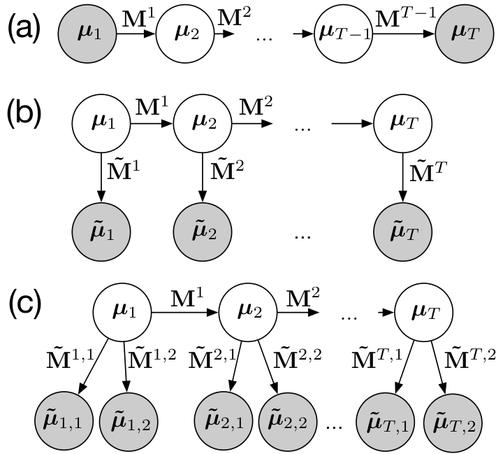
As shown in Fig. 2(b), given the noisy aggregated observations $\{\bm{\tilde{\mu}}_{t}\}_{t=1}^{T}$ ¹¹ 1 Hereafter, we use $\bm{\mu}_{t}$, ${\mathbf{M}}^{t}$ to denote the normalized observations $\bar{\bm{\mu}}_{t},\bar{\mathbf{M}}^{t}$, respectively, for ease of notation., the problem of estimating latent ensemble flows can be naturally reformulated as a convex optimization problem given by

where $\mathbf{\tilde{A}}$ denotes the emission parameter that determines the conditional distribution of the noisy observation $\bm{\tilde{\mu}}_{t}$ given the true marginal $\bm{\mu}_{t}$, and $\mathbf{\tilde{M}}^{t}$ refers to the transition flow between the true marginal $\bm{\mu}_{t}$ and the noisy observation $\bm{\tilde{\mu}}_{t}$.

where the cost tensor $\mathbf{C}\in\mathrm{R}^{S\times\cdots\times S}$ decomposes as $\mathbf{C}_{i_{1},\ldots,i_{J}}=\sum_{(u,v)\in E}\mathbf{C}^{(u,v)}_{i_{u},i_{v}}$, according to the tree structure in Fig. 2(b). The marginal observation $\bm{\mu}_{t}$ equals to the projection of the tensor-valued transport plan $\mathbf{M}\in\mathrm{R}^{S\times\cdots\times S}$ on its $t$-th mode. Similarly, the transition flow $\mathbf{M}^{t}$ can be obtained by the projection of the tensor-valued transport plan $\mathbf{M}$ on its $(t,t+1)$-th modes, i.e., $\mathbf{M}^{t}=P_{(t,t+1)}(\mathbf{M})$. We refer to Sec.4.2 in [9] for the detailed proof of the equivalence between Eq. 4.5 and 4.6.

As illustrated in Fig. 2(a), the multi-marginal optimal transport based methods [9, 11], aim to estimate the transition flow matrices $\{\mathbf{M}^{t}\}_{t=1}^{T-1}$ given the two marginal observations $\bm{\mu}_{1}$ and $\bm{\mu}_{T}$, using the predetermined transition matrix $\mathbf{A}$, for time-homogeneous Markov models. Fig. 2(b) illustrates a scenario in which the multiple noisy marginals are accessible. In particular, our goal is to simultaneously recover the transition flows $\{\mathbf{M}^{t}\}_{t=1}^{T-1}$ and to learn the unknown cost matrices $\{\mathbf{C}^{t}\}_{t=1}^{T-1}$ based upon the multiple marginal observations $\bm{\tilde{\mu}}_{t},\text{for}\ \ t=1,\ldots,T$. To this end, an EM-type algorithm is developed to solve the problem of estimating transition flows. More specifically, in the M-step, we consider learning the cost matrices $\mathbf{C}^{t(\ell)}$ of $\ell$-th iteration given the two marginal observations $\bm{\mu}_{t}$ and $\bm{\mu}_{t+1}$, and the estimated transition flow $\mathbf{M}^{t(\ell)}$ of the previous iteration. In the E-step, the expectation of transition flow $\mathbf{M}^{t(\ell+1)}$ is updated based upon $\mathbf{C}^{t(\ell)}$. Moreover, via the tree-structured MOT framework, the proposed method can be well extended to more complicated scenarios where multiple noisy aggregated observations are available for each marginal observation (Fig. 2(c)).

where $F(\bm{\alpha},\mathbf{C})\equiv\langle\mathbf{M}^{(\ell)},\mathbf{C}\rangle-\sum_{t}\langle\bm{\alpha_{t}},\bm{\mu}_{t}\rangle+\epsilon\langle\mathbf{K},\mathbf{B}\rangle$ is a convex function, $\bm{\alpha}\equiv[\bm{\alpha}_{1},\ldots,\bm{\alpha}_{T}]$ denote the dual variables corresponding to the marginal constraints $\{P_{t}(\mathbf{M})=\bm{\mu}_{t}\}_{t=1}^{T}$, $\mathbf{K}\equiv\exp(-\frac{\mathbf{C}}{\epsilon})$, $\mathbf{B}\equiv\mathbf{b}_{1}\otimes\cdots\otimes\mathbf{b}_{T}$ where $\mathbf{b}_{t}\equiv\exp(\frac{\bm{\alpha}_{t}}{\epsilon})$, and $R(\mathbf{C})$ is the regularization imposed on the cost tensor $\mathbf{C}$. The derivation of Eq. 4.7 is detailed in the appendix. Note that the optimization problem in Eq.4.7 admits infinitely many solutions without additional regularization imposing on cost tensor $\mathbf{C}$.

Some recent advancements [13, 16] in solving the problem of inverse optimal transport(IOT), has proved that the IOT problem admits an unique solution if the cost function is restricted to belong to a set of symmetric matrices with zero diagonal elements, and thus the proximal operator can be specified by

and followed by enforcing the diagonal entries of $\mathbf{C}^{t}$ to be $0$. In our case, the cost tensor of the inverse multi-marginal optimal transport problem, naturally decouples, according to the tree structure as $\mathbf{C}_{i_{1},\ldots,i_{J}}=\sum_{(u,v)\in\mathcal{E}}\mathbf{C}^{(u,v)}_{i_{u},i_{v}}$. Thus, we impose symmetric and zero-diagonal constraints straightforwardly on each of the cost matrices $\mathbf{C}^{t}$, instead of restricting a symmetric cost tensor. One instance of symmetric cost matrices is $\mathbf{C}^{t}=[{C}^{t}_{ij}]$ with ${C}^{t}_{ij}=|x_{i}-x_{j}|^{2}$ where $x_{i}$ and $x_{j}$ denote $i$-th and $j$-th locations, respectively. In particular, $\bm{\alpha}$ can be updated using Sinkhorn belief propagation algorithm for entropy regularized MOT. More specifically, to solve the convex optimization problem in Eq.4.7, a block coordinate descent scheme detailed in Algorithm 2 can be considered to alternatively update $\mathbf{C}$ and $\bm{\alpha}$.

Although the symmetric and zero-diagonal constraints ensure the unique solution, the cost matrices between the states might be more complex. For instance, in many urban population data [24], most individuals are transitioning from suburb towards downtown areas in the early morning, while they are moving back in the opposite direction, in the late evening. Inspired by recent advances in the optimal matching studies [4], we consider constructing the time-dependent cost matrices as a sparse, linear combination of basis distance matrices. More specifically, $\mathbf{C}^{t}=\sum_{q=1}^{Q}\beta^{t}_{q}\mathbf{D}^{q}$ where $\mathbf{D}_{ij}^{q}=|x_{i}-x_{j}|^{q}$ denotes the $(i,j)$-th element of the $q$-th basis distance matrix, $x_{i}$ is the $i$-th location, $\bm{\beta}^{t}=[\beta^{t}_{1},\ldots,\beta^{t}_{Q}]$ is a sparse coefficient vector with $q$-th element determining the usage of $\mathbf{D}^{q}$ in the construction of $\mathbf{C}^{t}$. Thus, the learning problem of the cost matrices $\mathbf{C}^{t}$ reduces to an optimization problem with respect to $\bm{\beta}^{t}$ and $\bm{\alpha}$ as

where $F(\bm{\alpha}^{t},\bm{\alpha}^{t+1},\bm{\beta})\equiv\sum_{i_{t},i_{t+1}}e^{[(\bm{\alpha}^{t})_{i_{t}}+(\bm{\alpha}^{t+1})_{i_{t+1}}-\mathbf{C}^{t}_{i_{t},i_{t+1}}]}+\sum_{i_{t},i_{t+1}}[\mathbf{C}^{t}_{i_{t},i_{t+1}}-(\bm{\alpha}^{t})_{i_{t}}-(\bm{\alpha}^{t+1})_{i_{t+1}}]$, and $\bm{\alpha}^{t},\bm{\alpha}^{t+1}$ denote the dual variables corresponding to $\bm{\mu}^{t},\bm{\mu}^{t+1}$, respectively, and the $\ell_{1}$ penalty term is to enforce a sparse coefficient vector $\bm{\beta}^{t}$. As we did in Algorithm 2, $\bm{\alpha}$ can be updated using Sinkhorn algorithm, and $\bm{\beta}$ is updated using an iterative shrinkage-thresholding algorithm (ISTA) [4], which leads to the second block coordinate descent scheme as detailed in Algorithm 3, for learning cost matrices. The proximal operator is given by the soft-thresholding operator specified by

The proposed EM-type algorithm is to estimate latent transition flows by iteratively implementing the Sinkhorn belief propagation in the E-step to estimate the expected transition flows, and to learn the cost functions using Algorithm 2 or Algorithm 3. Hereafter, we denote the two developed EM-type algorithms as Sinkhorn belief propagation inverse symmetric transport cost (SBP-ISTC), and Sinkhorn belief propagation iterative shrinkage-thresholding (SBP-ISTA) algorithms.

This paper proposed to estimate population transition flows from marginally aggregated data via a graphical-structured multi-marginal optimal transport framework. More specifically, the proposed methods allow the transition kernels behind population flows to be time-varying, by learning the time-dependent cost functions. The uniqueness of the solutions is guaranteed under mild conditions. The experiments on four real-world population flow data, show the improved accuracy of the proposed methods in estimating latent transition flows, compared with the others built upon time-homogeneous Markov chains.

References

- Akagi et al. [2020] Yasunori Akagi, Takuya Nishimura, Yusuke Tanaka, Takeshi Kurashima, and Hiroyuki Toda. Exact and efficient inference for collective flow diffusion model via minimum convex cost flow algorithm. In AAAI, pages 3163–3170, 2020.
- Benamou et al. [2015] Jean-David Benamou, Guillaume Carlier, Marco Cuturi, Luca Nenna, and Gabriel Peyre. Iterative Bregman projections for regularized transportation problems. SIAM J. Sci. Comput., 37(2):A1111–A1138, 2015.
- Bernstein and Sheldon [2016] Garrett Bernstein and Daniel Sheldon. Consistently estimating markov chains with noisy aggregate data. In AISTATS, pages 1142–1150, 2016.
- Carlier et al. [2020] Guillaume Carlier, Arnaud Dupuy, Alfred Galichon, and Yifei Sun. Sista: learning optimal transport costs under sparsity constraints. CoRR, 2020.
- Chang et al. [2021] Serina Chang, Emma Pierson, Pang Wei Koh, Jaline Gerardin, Beth Redbird, David Grusky, and Jure Leskovec. Mobility network models of covid-19 explain inequities and inform reopening. Nature, 589(7840):82–87, January 2021.
- Cuturi [2013] Marco Cuturi. Sinkhorn distances: Lightspeed computation of optimal transport. In NIPS, pages 2292–2300, 2013.
- Franklin and Lorenz [1989] Joel Franklin and Jens Lorenz. On the scaling of multidimensional matrices. Linear Algebra and its applications, 114:717–735, 1989.
- Haasler et al. [2019] Isabel Haasler, Axel Ringh, Yongxin Chen, and Johan Karlsson. Estimating ensemble flows on a hidden Markov chain. In CDC, pages 1331–1338, 2019.
- Haasler et al. [2021a] Isabel Haasler, Axel Ringh, Yongxin Chen, and Johan Karlsson. Multimarginal optimal transport with a tree-structured cost and the Schrödinger bridge problem. SIAM J. Control. Optim., 59(4):2428–2453, 2021.
- Haasler et al. [2021b] Isabel Haasler, Axel Ringh, Yongxin Chen, and Johan Karlsson. Scalable computation of dynamic flow problems via multi-marginal graph-structured optimal transport. CoRR, 2106.14485, 2021.
- Haasler et al. [2021c] Isabel Haasler, Rahul Singh, Qinsheng Zhang, Johan Karlsson, and Yongxin Chen. Multi-marginal optimal transport and probabilistic graphical models. IEEE Trans. Inf. Theory, 67(7):4647–4668, 2021.
- Iwata and Shimizu [2019] Tomoharu Iwata and Hitoshi Shimizu. Neural collective graphical models for estimating spatio-temporal population flow from aggregated data. In AAAI, pages 3935–3942, 2019.
- Li et al. [2019] Ruilin Li, Xiaojing Ye, Haomin Zhou, and Hongyuan Zha. Learning to match via inverse optimal transport. J. Mach. Learn. Res., 20:80:1–80:37, 2019.
- Luo et al. [2016] Dixin Luo, Hongteng Xu, Yi Zhen, Bistra Dilkina, Hongyuan Zha, Xiaokang Yang, and Wenjun Zhang. Learning mixtures of Markov chains from aggregate data with structural constraints. IEEE Transactions on Knowledge and Data Engineering, 28(6):1518–1531, 2016.
- Ma et al. [2021a] Shaojun Ma, Shu Liu, Hongyuan Zha, and Haomin Zhou. Learning stochastic behaviour from aggregate data. In ICML, pages 7258–7267, 2021.
- Ma et al. [2021b] Shaojun Ma, Haodong Sun, Xiaojing Ye, Hongyuan Zha, and Haomin Zhou. Learning cost functions for optimal transport. CoRR, 2021.
- Pass [2011] B. Pass. Uniqueness and Monge solutions in the multimarginal optimal transportation problem. SIAM Journal on Mathematical Analysis, 43(6):2758–2775, 2011.
- Pass [2012] B. Pass. On the local structure of optimal measures in the multi-marginal optimal transportation problem. Calc. Var. Partial Differential Equations, 43(3-4):529–536, 2012.
- Pele and Werman [2009] Ofir Pele and Michael Werman. Fast and robust earth mover’s distances. 2009 IEEE 12th International Conference on Computer Vision, pages 460–467, 2009.
- Ray [2020] Evan L Ray. Ensemble forecasts of Coronavirus disease 2019 (COVID-19) in the U.S. medRxiv, 2020.
- Sheldon and Dietterich [2011] Daniel R Sheldon and Thomas Dietterich. Collective graphical models. In NIPS, pages 1161–1169, 2011.
- Sheldon et al. [2013] Daniel Sheldon, Tao Sun, Akshat Kumar, and Thomas G. Dietterich. Approximate inference in collective graphical models. In ICML, pages 1004–1012, 2013.
- Singh et al. [2020a] Rahul Singh, Isabel Haasler, Qinsheng Zhang, Johan Karlsson, and Yongxin Chen. Inference with aggregate data: An optimal transport approach. CoRR, abs/2003.13933, 2020.
- Singh et al. [2020b] Rahul Singh, Qinsheng Zhang, and Yongxin Chen. Learning hidden Markov models from aggregate observations. CoRR, abs/2011.11236, 2020.
- Sun et al. [2015] Tao Sun, Daniel Sheldon, and Akshat Kumar. Message passing for collective graphical models. In ICML, pages 853–861, 2015.
- Tanaka et al. [2018] Yusuke Tanaka, Tomoharu Iwata, Takeshi Kurashima, Hiroyuki Toda, and Naonori Ueda. Estimating latent people flow without tracking individuals. In IJCAI, pages 3556–3563, 2018.
- Villani [2003] C. Villani. Topics in optimal transportation theory. 01 2003.
- Wang et al. [2016] Yichen Wang, Evangelos A. Theodorou, Apurv Verma, and Le Song. Steering opinion dynamics in information diffusion networks. CoRR, 2016.
- Yuan et al. [2013] Jing Yuan, Yu Zheng, Xing Xie, and Guangzhong Sun. T-drive: Enhancing driving directions with taxi drivers’ intelligence. IEEE Trans. on Knowl. and Data Eng., 25(1):220–232, jan 2013.