跳到论文正文
W Papers独立论文阅读器 arXiv:2212.14411 论文正文 计算阅读时间 · 0%
引用这篇论文根据当前论文元数据生成,正式投稿前建议核对。


License: arXiv.org perpetual non-exclusive license
arXiv:2212.14411v5 [stat.ME] 11 Mar 2024

Near-Optimal, Near-Calibrated, Non-Parametric Sequential Tests and Confidence Sequences with Possibly Dependent Observations

Aurélien Bibaut    Nathan Kallus    Michael Lindon
1Netflix  2Cornell University
Abstract

Sequential tests and their implied confidence sequences, which are valid at arbitrary stopping times, promise flexible statistical inference and on-the-fly decision making. However, strong guarantees are limited to parametric sequential tests that under-cover in practice or concentration-bound-based sequences that over-cover and have suboptimal rejection times. In this work, we consider classic delayed-start normal-mixture sequential probability ratio tests, and we provide the first asymptotic type-I-error and expected-rejection-time guarantees under general non-parametric data generating processes, where the asymptotics are indexed by the test’s burn-in time. The type-I-error results primarily leverage a martingale strong invariance principle and establish that these tests (and their implied confidence sequences) have type-I error rates asymptotically equivalent to the desired (possibly varying) α\alpha-level. The expected-rejection-time results primarily leverage an identity inspired by Itô’s lemma and imply that, in certain asymptotic regimes, the expected rejection time is asymptotically equivalent to the minimum possible among α\alpha-level tests. We show how to apply our results to sequential inference on parameters defined by estimating equations, such as average treatment effects. Together, our results establish these (ostensibly parametric) tests as general-purpose, non-parametric, and near-optimal. We illustrate this via numerical simulations and a real-data application to A/B testing at Netflix.

1 Introduction

Inference based on randomized experiments forms the basis of important decisions in an incredibly diverse range of domains, from medicine (Schulz et al. 2010) to development economics (Banerjee et al. 2015) to technology business (Tingley et al. 2021). Toward the aim of making better and faster decisions, it is particularly helpful for statistical procedures to be flexible (Grünwald et al. 2020). Experimental designs which require a pre-specified sample size can be quite rigid in practice. For example, unless some oracle information is known about the effect size, such designs will ultimately include some over- or under-experimentation; collecting more samples than necessary when the treatment effect is under-estimated, and not collecting enough when over-estimated. Sequential designs, on the other hand, enable faster decision-making as they support the ability to analyze data as and when it arrives, enabling us to stop experimenting when the data strongly supports a conclusion. The ability to continuously monitor experiments in turn leads to better decisions, as it prevents bad practices that arise from attempting to use more rigid statistical procedures in applications where resources and schedules often change dynamically.

1.1 The sequential testing framework

The sequential testing problem can in general be modelled by the following framework, which encompasses most settings from the literature we refer to. The analyst receives a stream of random data points X1,X2,…X_{1},X_{2},\ldots, all lying in a certain set 𝒳\mathcal{X}, adapted to a filtration 𝔉=(ℱt)t≥1\mathfrak{F}=(\mathcal{F}_{t})_{t\geq 1}. For any t≥1t\geq 1, we denote ψt=E⁡[Xt∣ℱt−1]\psi_{t}=E[X_{t}\mid\mathcal{F}_{t-1}] the conditional mean of XtX_{t} given previous observations. We consider the problem of testing the statistical hypothesis H0H_{0} that ψt=ψ0′\psi_{t}=\psi^{\prime}_{0} for every t≥1t\geq 1, for some ψ0′∈ℝ\psi^{\prime}_{0}\in\mathbb{R}, against the composite alternative H~\0:∪ψ1′≠ψ0′H~(ψ1′)\widetilde{H}_{\backslash 0}:\cup_{\psi^{\prime}_{1}\neq\psi^{\prime}_{0}}\widetilde{H}(\psi^{\prime}_{1}), where H~​(ψ1′):limt→∞ψt=ψ1′\widetilde{H}(\psi^{\prime}_{1}):\lim_{t\to\infty}\psi_{t}=\psi^{\prime}_{1}. In words, H~\0\widetilde{H}_{\backslash 0} is the hypothesis that ψt\psi_{t} has a limit, and that this limit is not ψ0′\psi^{\prime}_{0}. A sequential test is an 𝔉\mathfrak{F}-adapted stopping time τ\tau. If τ=t\tau=t for some t<∞t<\infty, we say that the sequential time rejects H0H_{0} at tt, while if τ=∞\tau=\infty, we say that the test doesn’t reject H0H_{0}.

1.2 Challenges of sequential testing and limitations of the state of the art

Analyzing data in this fashion requires special inference that explicitly accounts for the sequential nature of the decision-making process. It is well known that repeated application of classical significance tests to accumulating sets of data results in procedures with drastically inflated type-I error rates (Armitage et al. 1969). Even under the null hypothesis, the absolute value of the tt-statistic applied to an independent and identically distributed (i.i.d.) sequence is guaranteed to fall into the rejection region at some point, regardless of the chosen α\alpha-level (Strassen 1964). An analyst intent on disproving any one hypothesis can keep collecting data until this occurs.

For these reasons, a long line of literature has explored sequential testing and confidence sequences. However, we claim that the existing literature still does not provide all the guarantees necessary for the widespread use of confidence sequences and sequential tests in statistical practice. We believe indeed that practitioners would want to know three things before adopting them.

  • •

    Is type-I error, or equivalently, coverage guaranteed to hold at the predetermined level α\alpha?

  • •

    Is the procedure sample efficient? In particular, is its expected sample size unimprovable among all level-α\alpha sequential tests?

  • •

    Is the procedure non-parametric? Indeed, practitioners aren’t (or at least shouldn’t be) willing to make parametric assumptions, which we believe are unrealistic in most settings.

In our understanding, the prevailing view is that practitioners have essentially two choices at their disposal. One is to use parametric-model-based confidence sequences which tend to under-cover and over-reject. The other is to use concentration-inequalities-based sequences, which tend to over-cover and under-reject. A prominent example of parametric confidence sequences is the mixture SPRT boundaries for Brownian data sequences introduced by Robbins and Siegmund 1970 and further refined in (Robbins 1970). Notable contributions to the field of concentration-inequality-based sequences include Howard et al. 2021 and Howard and Ramdas 2022.

These two types of sequences are not actually the only options but the alternatives may be less well-known as of now. These alternatives are asymptotic in nature and are based on weak and strong invariance principles (WIPs and SIPs). Robbins and Siegmund 1970 propose a sequence of delayed-start mixture SPRT boundaries and show, via Donsker’s WIP, that coverage tends to α\alpha as the delay before the start of monitoring diverges to infinity. More recently, Bibaut et al. 2021c use McLeish 1974’s WIP to provide a sequence of delayed-start confidence sequences for dependent data. Waudby-Smith et al. 2021 propose a novel definition of asymptotic confidence sequences and demonstrate how SIPs allow to construct such asymptotic sequences. The advantage of these WIP- and SIP-based sequences (or sequences of sequences) is that they hold the promise of tight type-I error control (as opposed to over or anti-conservativity) under minimal assumptions – typically mere moment assumptions. We discuss more in detail why going for an asymptotic WIP-based or SIP-based solution is the right strategy in the next subsection.

Nevertheless, we claim that, as of the time of writing of this article, no existing work simultaneously proposes confidence sequences and an analysis showing that these satisfy the aforementioned three criteria. In particular, we discuss in Section 10.5 how the current work compares to Waudby-Smith et al. 2021 in that respect.

1.3 The case for an asymptotic procedure

In fixed-sample-size inference, arguably the most used procedure is to construct approximate central-limit-theorem- (CLT) based confidence intervals. The central limit theorem and extensions thereof only require a second-order moment (or a Lindeberg or Lyapunov condition), and allow for an extremely wide range of data-generating processes. The coverage error one makes by using a CLT-based confidence intervals is controlled by Berry-Esseen bounds and decreases rapidly, scaling as the inverse square root of the sample size (provided the observations have a third moment).

Comparatively, parametric-model-based confidence sequences and nonparametric concentration bounds aren’t as commonly used in applied statistical practice for the same reasons we mentioned for confidence sequences: the former become anti-conservative as soon as the parametric assumptions do not hold, while the latter are over-conservative in general.

This therefore motivates looking for a CLT-like solution to sequential inference and testing. Fortunately, there exist sequential extensions of CLT results: these are precisely the WIPs and the SIPs we mentioned above. These guarantee convergence (in distribution and almost surely, respectively) of partial sum processes to Gaussian processes, under weak moment assumptions.

1.4 Aim of the current paper

We aim to justify the use of existing sequential tests and the corresponding confidence sequences, namely the delayed-start versions (Robbins and Siegmund 1974) of the running maximum likelihood SPRT (rmlSPRT) (Robbins and Siegmund 1972; Robbins and Siegmund 1974), and the normal mixture SPRT (nmSPRT). In other words, we give guarantees supporting that it is safe, efficient, and advisable to use these. We show that, under mild non-parametric assumptions, sequences of these sequential tests indexed by the burn-in time (1) have type-I error converging asymptotically to the prespecified level, and (2) have expected stopping time converging to the lower bounds known in the i.i.d. case both in the regime where ψ1′→ψ0′\psi_{1}^{\prime}\to\psi_{0}^{\prime}, and in the regime where α→0\alpha\to 0.

1.5 Contributions and organization of this article

We show in Section 3 that the type-I error of delayed-start nmSPRTs and rmlSPRTs converges to α\alpha as burn-in time goes to infinity. We show in Section 5 that, in our non-parametric dependent setting, in the asymptotic regime where α→0\alpha\to 0, the expected rejection time is asymptotically equivalent, up to a small constant, to the lower bound known for simple-vs-simple SPRTs under parametric i.i.d. data. We also show that, in the asymptotic regime where the effect size ψ1′−ψ0′\psi^{\prime}_{1}-\psi^{\prime}_{0} converges to 0, the expected stopping time converges, up to a constant factor, to the lower bound known in the parametric i.i.d. setting. We propose in Section 6 a sample splitting and variance stabilization method to conduct estimating-equations-based inference under sequentially collected data. In Section 7, we study heuristically the optimal choice of the hyperparameter in nmSPRTs, and we propose a heuristic procedure that auto-tunes this hyperparameter. In Section 8 we conduct extensive simulation studies so as to demonstrate numerically the validity of our theoretical results and the empirical robustness of our heuristic auto-tuned nmSPRTs, and in Section 9 we study a real-data application to A/B testing for quality control of the Netflix client application. In Section 10 we review the historical and logical progression from Wald 1945’s simple-vs-simple SPRT to the results we present in this paper. In Section 11 we further discuss the related literature.

2 Setup

We work in the sequential setting introduced in Section 1.1. For any t≥1t\geq 1, we denote St=∑s=1tXsS_{t}=\sum_{s=1}^{t}X_{s}. Our methods are designed to work with observations for which the conditional variance given the past converges to one. We will make rigorous what are the specific variance convergence requirements in the upcoming sections, but it might be helpful to think throughout of Var⁡(Xt∣ℱt−1)\mathrm{Var}(X_{t}\mid\mathcal{F}_{t-1}) as being approximately one.

For any t≥1t\geq 1, and λ>0\lambda>0, we define the rmlSPRT and nmSPRT statistics as

YtrmlSPRT=12​(St2t−log⁡t)andYλ,tnmSPRT=12​(St2t+λ−log⁡t+λλ).\displaystyle Y_{t}^{\mathrm{rmlSPRT}}=\frac{1}{2}\left(\frac{S_{t}^{2}}{t}-\log t\right)\qquad\text{and}\qquad Y_{\lambda,t}^{\mathrm{nmSPRT}}=\frac{1}{2}\left(\frac{S_{t}^{2}}{t+\lambda}-\log\frac{t+\lambda}{\lambda}\right). (2)

We refer the reader to Section 10 for the motivation behind the expressions of the test statistics and the rationale of their names.

So as to avert any confusion, the reader should keep in mind that while we present the guarantees for both test statistics along one another, the analyst will opt for one of the two and monitor only the chosen one (as opposed for instance to monitoring which of the two crosses a given threshold first, or any variation thereof). Let t0≥1t_{0}\geq 1 be the burn-in period, that is the time the analyst waits before starting to monitor whether the test statistic crosses a certain rejection threshold. We will justify that for burn-in period t0t_{0} (and parameter λ\lambda for the nmSPRT), the “right” rejection thresholds for the rmlSPRT and the nmSPRT are −log⁡α~1​(α)-\log\widetilde{\alpha}_{1}(\alpha) and −log⁡α~2,λ/t0​(α)-\log\widetilde{\alpha}_{2,\lambda/t_{0}}(\alpha), respectively, where α~1​(α)\widetilde{\alpha}_{1}(\alpha) solves h1​(−log⁡α~1)=αh_{1}(-\log\widetilde{\alpha}_{1})=\alpha and, for any η>0\eta>0, α~2,η​(α)\widetilde{\alpha}_{2,\eta}(\alpha) solves h2,η​(−log⁡α~2,η)=αh_{2,\eta}(-\log\widetilde{\alpha}_{2,\eta})=\alpha, where

h1​(a)=\displaystyle h_{1}(a)= 2​exp⁡(−a)​aπ+2​(1−Φ⁡(2​a)),\displaystyle 2\exp(-a)\sqrt{\frac{a}{\pi}}+2\left(1-\Phi\left(\sqrt{2a}\right)\right), (3)
andh2,η​(a)=\displaystyle\text{and}\qquad h_{2,\eta}(a)= exp⁡(−a)​{2​Φ​(2​η​(a+12​log⁡1+ηη))−1}\displaystyle\exp(-a)\left\{2\Phi\left(\sqrt{2\eta\left(a+\frac{1}{2}\log\frac{1+\eta}{\eta}\right)}\right)-1\right\} (4)
+2​{1−Φ⁡(2​(1+η)​(a+12​log⁡1+ηη))}.\displaystyle+2\left\{1-\Phi\left(\sqrt{2(1+\eta)\left(a+\frac{1}{2}\log\frac{1+\eta}{\eta}\right)}\right)\right\}. (5)

The combination of a test statistic, a burn-in period, and a rejection level specifies a sequential test. Formally we define the the t0t_{0}-burn-in rmlSPRT and nmSPRT as the stopping times

τrmlSPRT​(α,t0)=\displaystyle\tau^{\mathrm{rmlSPRT}}(\alpha,t_{0})= inf{t≥t0:YtrmlSPRT≥−log⁡α~1​(α)},\displaystyle\inf\left\{t\geq t_{0}:Y_{t}^{\mathrm{rmlSPRT}}\geq-\log\widetilde{\alpha}_{1}(\alpha)\right\}, (6)
andτnmSPRT​(α,λ,t0)=\displaystyle\text{and}\qquad\tau^{\mathrm{nmSPRT}}(\alpha,\lambda,t_{0})= inf{t≥t0:Yλ,tnmSPRT≥−log⁡α~2,λ/t0​(α)}.\displaystyle\inf\left\{t\geq t_{0}:Y_{\lambda,t}^{\mathrm{nmSPRT}}\geq-\log\widetilde{\alpha}_{2,\lambda/t_{0}}(\alpha)\right\}. (7)

For any t≥1t\geq 1, we define 𝒞α,t0rmlSPRT​(t)\mathcal{C}^{\mathrm{rmlSPRT}}_{\alpha,t_{0}}(t) (resp. 𝒞α,λ,t0nmSPRT​(t)\mathcal{C}^{\mathrm{nmSPRT}}_{\alpha,\lambda,t_{0}}(t)) as the set of values ψ0′∈ℝ\psi^{\prime}_{0}\in\mathbb{R} for which the rmlSPRT (resp. the nmSPRT) doesn’t reject at tt the hypothesis H0:ψt=ψ0′​∀tH_{0}:\psi_{t}=\psi^{\prime}_{0}\ \forall t. It is then straightforward to observe that the sequences (𝒞α,t0rmlSPRT​(t))t≥1(\mathcal{C}^{\mathrm{rmlSPRT}}_{\alpha,t_{0}}(t))_{t\geq 1} and (𝒞α,λ,t0nmSPRT​(t))t≥1(\mathcal{C}^{\mathrm{nmSPRT}}_{\alpha,\lambda,t_{0}}(t))_{t\geq 1} have coverage equal to 1 minus the level of the corresponding tests. Inverting the expressions of the test statistics yields that, for t≥t0t\geq t_{0}, 𝒞α,t0rmlSPRT​(t)=[±cα,t0rmlSPRT​(t)]\mathcal{C}^{\mathrm{rmlSPRT}}_{\alpha,t_{0}}(t)=[\pm c^{\mathrm{rmlSPRT}}_{\alpha,t_{0}}(t)] and 𝒞α,λ,t0nmSPRT​(t)=[±cα,λ,t0nmSPRT​(t)]\mathcal{C}^{\mathrm{nmSPRT}}_{\alpha,\lambda,t_{0}}(t)=[\pm c^{\mathrm{nmSPRT}}_{\alpha,\lambda,t_{0}}(t)] with

cα,t0rmlSPRT​(t)=\displaystyle c^{\mathrm{rmlSPRT}}_{\alpha,t_{0}}(t)= t⁡(−2​log⁡α~1​(α)+log⁡tt0)\displaystyle\sqrt{t\left(-2\log\widetilde{\alpha}_{1}(\alpha)+\log\frac{t}{t_{0}}\right)} (8)
andcα,λ,t0nmSPRT​(t)=\displaystyle\text{and}\qquad c^{\mathrm{nmSPRT}}_{\alpha,\lambda,t_{0}}(t)= (t+λ)​(−2​log⁡α~2,λ/t0​(α)+log⁡t+λλ).\displaystyle\sqrt{(t+\lambda)\left(-2\log\widetilde{\alpha}_{2,\lambda/t_{0}}(\alpha)+\log\frac{t+\lambda}{\lambda}\right)}. (9)

We now present two applications that exemplify our setting and the use of the delayed-start confidence sequences.

Example 1 (Sample mean).

Suppose we sequentially observe an i.i.d. scalar sequence Z1,Z2,…Z_{1},Z_{2},\dots with common mean θ=E⁡[Z1]\theta=E[Z_{1}]. So as to ensure that the conditional variance of the data we use as input of the testing procedure converges to 1, we use a variance stabilization device. Specifically we set σ^t2\widehat{\sigma}^{2}_{t} to be the empirical variance of Z1,…,ZtZ_{1},\ldots,Z_{t}, that is σ^t2=(t−1)−1​∑s=1t(Zs−Z¯t)2\widehat{\sigma}^{2}_{t}=(t-1)^{-1}\sum_{s=1}^{t}(Z_{s}-\bar{Z}_{t})^{2}, with Z¯t=t−1​∑s=1tZt\bar{Z}_{t}=t^{-1}\sum_{s=1}^{t}Z_{t}. Then, to test θ=θ0\theta=\theta_{0} for a given θ0\theta_{0}, we set Xt=ωt​(Zt−θ0)X_{t}=\omega_{t}(Z_{t}-\theta_{0}), where ωt=(σ^t−1∨t−ι)−1\omega_{t}=(\widehat{\sigma}_{t-1}\vee t^{-\iota})^{-1}, for some ι>0\iota>0 such that t−ιt^{-\iota} is a time-decreasing threshold that ensures that ωt\omega_{t} is finite. To construct a confidence sequence for θ\theta, we consider all θ0\theta_{0}’s not rejected at time tt. Namely, letting Γt=∑s=1tωs\Gamma_{t}=\sum_{s=1}^{t}\omega_{s}, θ^t=Γt−1​∑s=1tωs​Zs\widehat{\theta}_{t}=\Gamma_{t}^{-1}\sum_{s=1}^{t}\omega_{s}Z_{s}, the delayed-start running MLE and the normal-mixture SPRT confidence sequences are

ℝ​ for ​t<t0 and [θ^t±Γt−1​cα,t0rmlSPRT​(t)]for ​t≥t0,\displaystyle\mathbb{R}\text{ for }t<t_{0}\qquad\text{ and }\qquad\left[\widehat{\theta}_{t}\pm\Gamma_{t}^{-1}c^{\mathrm{rmlSPRT}}_{\alpha,t_{0}}(t)\right]\qquad\text{for }t\geq t_{0}, (10)
and ℝ​ for ​t<t0 and [θ^t±Γt−1​cα,λ,t0nmSPRT​(t)]for ​t≥t0,\displaystyle\mathbb{R}\text{ for }t<t_{0}\qquad\text{ and }\qquad\left[\widehat{\theta}_{t}\pm\Gamma_{t}^{-1}c^{\mathrm{nmSPRT}}_{\alpha,\lambda,t_{0}}(t)\right]\qquad\text{for }t\geq t_{0}, (11)

respectively. Our results provide guarantees about the probability that θ\theta is ever excluded from this interval at any time and the expected time until any one θ′≠θ\theta^{\prime}\neq\theta is excluded.

Example 2 (Bernoulli trial with covariates).

Suppose we conduct a randomized controlled trial with two arms, in which we enroll patients sequentially. Upon enrolling the tt-th patient, we collect a vector of pre-treatment covariates Lt∈ℝdL_{t}\in\mathbb{R}^{d} (potentially d=0d=0 if we do not collect or opt not to use covariates), we randomly sample their treatment arm allocation At∈{0,1}A_{t}\in\{0,1\} from a Bernoulli distribution with mean p∈(0,1)p\in(0,1), and we then observe their health outcome Ut∈ℝU_{t}\in\mathbb{R}. We suppose that the triples (L1,A1,U1),(L2,A2,U2),…(L_{1},A_{1},U_{1}),\allowbreak(L_{2},A_{2},U_{2}),\allowbreak\ldots are i.i.d. Let the statistical parameter of interest be θ=E⁡[U1∣A1=1]−E⁡[U1∣A1=0]\theta=E[U_{1}\mid A_{1}=1]-E[U_{1}\mid A_{1}=0]. For inference on θ\theta, set

Zt=η^t−1​(1,Lt)−η^t−1​(0,Lt)+At−pp⁡(1−p)​(Ut−η^t−1​(At,Lt))\displaystyle Z_{t}=\widehat{\eta}_{t-1}(1,L_{t})-\widehat{\eta}_{t-1}(0,L_{t})+\frac{A_{t}-p}{p(1-p)}\left(U_{t}-\widehat{\eta}_{t-1}(A_{t},L_{t})\right) (12)

where η^t−1\widehat{\eta}_{t-1} is an ℱt−1\mathcal{F}_{t-1}-measurable estimate of the outcome regression function η:(a,l)↦E[U1∣A1=a,L1=l]\eta:(a,l)\mapsto E[U_{1}\mid A_{1}=a,L_{1}=l], set σ^t−12\widehat{\sigma}^{2}_{t-1} to be an ℱt−1\mathcal{F}_{t-1} measurable estimate of Var⁡(Zt∣η^t−1)\mathrm{Var}(Z_{t}\mid\widehat{\eta}_{t-1}) and apply the approach from Example 1.

3 Type I error

Characterizing the type-I error of the delayed start rmlSPRT and nmSPRT is a priori easier if the data distribution under the null is known. As invariance principles guarantee convergence of partial sum processes of general nonparametric centered data sequences to Wiener (a.k.a. Brownian) processes, we start our type-I error study by characterizing the distributional properties of the test statistics under Brownian data. Let W=(W⁡(t))t≥0W=(W(t))_{t\geq 0} be a Wiener process adapted to a filtration 𝔉~=(ℱ~​(t))t≥0\widetilde{\mathfrak{F}}=(\widetilde{\mathcal{F}}(t))_{t\geq 0}. Let Y~trmlSPRT\widetilde{Y}_{t}^{\mathrm{rmlSPRT}} and Y~λ,tnmSPRT\widetilde{Y}_{\lambda,t}^{\mathrm{nmSPRT}} be the Brownian-data counterparts of YtrmlSPRTY_{t}^{\mathrm{rmlSPRT}} and Yλ,tnmSPRTY_{\lambda,t}^{\mathrm{nmSPRT}}:

Y~trmlSPRT=12​(W​(t)2t−log⁡t)andY~λ,tnmSPRT=12​(W​(t)2t+λ−log⁡t+λλ).\displaystyle\widetilde{Y}_{t}^{\mathrm{rmlSPRT}}=\frac{1}{2}\left(\frac{W(t)^{2}}{t}-\log t\right)\qquad\text{and}\qquad\widetilde{Y}_{\lambda,t}^{\mathrm{nmSPRT}}=\frac{1}{2}\left(\frac{W(t)^{2}}{t+\lambda}-\log\frac{t+\lambda}{\lambda}\right). (13)

The following result shows that choices α~1​(α)\widetilde{\alpha}_{1}(\alpha) and α~2,λ/t0​(α)\widetilde{\alpha}_{2,\lambda/t_{0}}(\alpha) above ensure that −log⁡α~1​(α)-\log\widetilde{\alpha}_{1}(\alpha) and −log⁡α~2,λ/t0​(α)-\log\widetilde{\alpha}_{2,\lambda/t_{0}}(\alpha) are (1−α)(1-\alpha)-boundaries for the Brownian test statistics Y~trmlSPRT\widetilde{Y}_{t}^{\mathrm{rmlSPRT}} and Y~λ,tnmSPRT\widetilde{Y}_{\lambda,t}^{\mathrm{nmSPRT}} when monitored continuously in time at all t≥t0t\geq t_{0}.

Lemma 1.

For any t0≥1t_{0}\geq 1 and λ>0\lambda>0,

P[supt≥t0Y~trmlSPRT+12logt0≥−logα~1(α)]=α\displaystyle P\left[\sup_{t\geq t_{0}}\widetilde{Y}_{t}^{\mathrm{rmlSPRT}}+\frac{1}{2}\log t_{0}\geq-\log\widetilde{\alpha}_{1}(\alpha)\right]=\alpha (14)
and P[supt≥t0Y~λ,tnmSPRT≥−logα~2,λ/t0(α)]=α.\displaystyle P\left[\sup_{t\geq t_{0}}\widetilde{Y}_{\lambda,t}^{\mathrm{nmSPRT}}\geq-\log\widetilde{\alpha}_{2,\lambda/t_{0}}(\alpha)\right]=\alpha. (15)

Equivalently,

P[∀t≥t0,W(t)∈𝒞α,t0rmlSPRT(t)]=1−α\displaystyle P\left[\forall t\geq t_{0},\ W(t)\in\mathcal{C}^{\mathrm{rmlSPRT}}_{\alpha,t_{0}}(t)\right]=1-\alpha (16)
and P[∀t≥t0,W(t)∈𝒞α,λ,t0nmSPRT(t)]=1−α.\displaystyle P\left[\forall t\geq t_{0},\ W(t)\in\mathcal{C}^{\mathrm{nmSPRT}}_{\alpha,\lambda,t_{0}}(t)\right]=1-\alpha. (17)

The claims on Y~λ,tnmSPRT\widetilde{Y}^{\mathrm{nmSPRT}}_{\lambda,t} and 𝒞α,λ,t0nmSPRT\mathcal{C}^{\mathrm{nmSPRT}}_{\alpha,\lambda,t_{0}} are a direct consequence of Theorem 2 in Robbins and Siegmund 1970. The claims on Y~trmlSPRT\widetilde{Y}_{t}^{\mathrm{rmlSPRT}} and 𝒞α,t0rmlSPRT\mathcal{C}^{\mathrm{rmlSPRT}}_{\alpha,t_{0}} follow from similar techniques. Version 7 of Waudby-Smith et al. 2021 also includes a proof of these. We include a proof of Lemma 1 in the appendix for self-containedness.

We now show that type-I error converges along any joint sequence of rmlSPRTs or nmSPRTs and of values of α\alpha, such that the burn-in time t0t_{0} diverges to ∞\infty. The guarantees will hold even with discrete-time, non-normal, dependent observations. The proof hinges on constructing a joint probability space for both these observations and the continuous-time Brownian motion, in which supt≥t0|Y~trmlSPRT−YtrmlSPRT|\sup_{t\geq t_{0}}|\widetilde{Y}_{t}^{\mathrm{rmlSPRT}}-Y_{t}^{\mathrm{rmlSPRT}}| and supt≥t0|Y~λ,tnmSPRT−Yλ,tnmSPRT|\sup_{t\geq t_{0}}|\widetilde{Y}_{\lambda,t}^{\mathrm{nmSPRT}}-Y_{\lambda,t}^{\mathrm{nmSPRT}}| are small. Almost-sure approximations of partial sums by Brownian motions under lax conditions are the object of strong invariance principles. We will specifically leverage the SIP result from theorem 1.3 of Strassen 1967. To do so, we impose the following conditions.

Assumption 1.

Let Vt=∑s=1tvsV_{t}=\sum_{s=1}^{t}v_{s}. For some non-decreasing function f:[0,∞)→(0,∞)f:[0,\infty)\to(0,\infty) such that f⁡(t)=O⁡(t​(log⁡t)−4​(log⁡log⁡t)−2)f(t)=O(t(\log t)^{-4}(\log\log t)^{-2}), it holds that

∑t=1∞1f⁡(Vt)E[(Xt−ψt)2𝟏{(Xt−ψt)2>f(Vt)}∣ℱt−1]<∞,\displaystyle\sum_{t=1}^{\infty}\frac{1}{f(V_{t})}E\left[\left(X_{t}-\psi_{t}\right)^{2}\bm{1}\left\{(X_{t}-\psi_{t})^{2}>f(V_{t})\right\}\mid\mathcal{F}_{t-1}\right]<\infty, (18)

and

Vt−t=o⁡(t​f​(t)​log⁡t)almost surely.\displaystyle V_{t}-t=o\left(\sqrt{tf(t)}\log t\right)\qquad\text{almost surely.} (19)

For now, we take 1 as a primitive assumption. In Section 6, we will discuss simple sufficient conditions for it for the case of stabilized estimating equations. Condition (18) is akin to (but different from) a martingale Lindeberg condition, and in Section 6 we satisfy it by assuming a moment higher than 2 exists.

A SIP guarantee is, of course, asymptotic, so we need to consider regimes where the stopping time is large. One such regime is when we set a long burn-in period t0t_{0}, essentially to wait for the data to look normal. The following theorem provides a type-I error guarantee (equivalently, a coverage guarantee) along sequences ((,,,,,))m≥1((t_{0,m},\alpha_{m},\lambda_{m}))_{m\geq 1} such that t0,m→∞t_{0,m}\to\infty.

Theorem 1.

Suppose that 1 holds. Then, for any sequence ((,,,,,))m≥1((t_{0,m},\allowbreak\alpha_{m},\allowbreak\lambda_{m}))_{m\geq 1} such that t0,m→∞t_{0,m}\to\infty, λm>0\lambda_{m}>0, αm∈[0,1]\alpha_{m}\in[0,1] ∀m≥1\forall m\geq 1,

limm→∞Pr[∃t≥t0,m,YtrmlSPRT+12logt0,m≥−logα~1(αm)]/αm=1,\displaystyle\lim_{m\to\infty}\Pr\left[\exists t\geq t_{0,m},\ Y^{\mathrm{rmlSPRT}}_{t}+\frac{1}{2}\log t_{0,m}\geq-\log\widetilde{\alpha}_{1}(\alpha_{m})\right]/\alpha_{m}=1, (20)
and limm→∞Pr[∃t≥t0,m,Yλm,tnmSPRT≥−logα~2,λm/t0,m(αm)]/αm=1.\displaystyle\lim_{m\to\infty}\Pr\left[\exists t\geq t_{0,m},\ Y^{\mathrm{nmSPRT}}_{\lambda_{m},t}\geq-\log\widetilde{\alpha}_{2,\lambda_{m}/t_{0,m}}(\alpha_{m})\right]/\alpha_{m}=1. (21)

Equivalently,

limm→∞Pr[∃t≥t0,m,St∉𝒞αm,t0,mrmlSPRT(t)]/αm=1,\displaystyle\lim_{m\to\infty}\Pr\left[\exists t\geq t_{0,m},\ S_{t}\not\in\mathcal{C}^{\mathrm{rmlSPRT}}_{\alpha_{m},t_{0,m}}(t)\right]/\alpha_{m}=1, (22)
and limm→∞Pr[∃t≥t0,m,St∉𝒞αm,λm,t0,mnmSPRT(t)]/αm=1.\displaystyle\lim_{m\to\infty}\Pr\left[\exists t\geq t_{0,m},\ S_{t}\not\in\mathcal{C}^{\mathrm{nmSPRT}}_{\alpha_{m},\lambda_{m},t_{0,m}}(t)\right]/\alpha_{m}=1. (23)

4 Representation of boundaries as inverted running-effect-size-estimate SPRTs

Before presenting our representation results for the rmlSPRT and nmSPRT statistics, let us first discuss known related facts. Let S~​(t)=ψ~​t+W​(t)\widetilde{S}(t)=\widetilde{\psi}t+W(t) be a time-continuous Brownian observation sequence with constant drift ψ~\widetilde{\psi}. Robbins and Siegmund 1974 show via Itô’s lemma that, under input data process S~\widetilde{S}, the nmSPRT test statistic Y~λ,tnmSPRT=12​{S~2​(t)/(t+λ)−log⁡((t+λ)/λ)}\widetilde{Y}^{\mathrm{nmSPRT}}_{\lambda,t}=\frac{1}{2}\{\widetilde{S}^{2}(t)/(t+\lambda)-\log((t+\lambda)/\lambda)\} can be represented alternatively as Y~λ,tnmSPRT=∫0tψ~λ​(s)​𝑑S~​(s)−12​ψ~λ2​(s)​𝑑s\widetilde{Y}^{\mathrm{nmSPRT}}_{\lambda,t}=\int_{0}^{t}\widetilde{\psi}_{\lambda}(s)d\widetilde{S}(s)-\frac{1}{2}\widetilde{\psi}_{\lambda}^{2}(s)ds, where ψ~λ​(t)=S~​(t)/(t+λ)\widetilde{\psi}_{\lambda}(t)=\widetilde{S}(t)/(t+\lambda) is the posterior mean of the drift ψ~\widetilde{\psi} under prior 𝒩⁡(0,1/λ)\mathcal{N}(0,1/\lambda). We refer to this latter representation as a running-posterior-mean SPRT. In the same article, they discuss the stopping time properties of a related test of which the test statistic is ∫0tψ~0​(s)​𝑑S~​(s)−12​ψ~02​(s)​𝑑s\int_{0}^{t}\widetilde{\psi}_{0}(s)d\widetilde{S}(s)-\frac{1}{2}\widetilde{\psi}^{2}_{0}(s)ds. Observing that ψ~0​(t)\widetilde{\psi}_{0}(t) is the maximum likelihood estimate of ψ~\widetilde{\psi}, we refer to this latter test statistic as a running-maximum-likelihood-estimate SPRT. As Robbins and Siegmund 1974 observe, these running-effect-size-estimate SPRT representations are amenable to rejection time analysis. This motivates us to look for such representations of the rmlSPRT and nmSPRT statistics.

While we cannot directly apply Itô’s lemma in our nonparametric discrete-time setting, we derive a finite-differences equivalent of a certain Itô-derived identity, namely that for hλ​(x,t)=12​x2/(t+λ)h_{\lambda}(x,t)=\frac{1}{2}x^{2}/(t+\lambda), d​hλ​(S~​(t),t)=ψ~λ​(t)​d​S~​(t)−12​ψ~λ2​(t)+12​(t+λ)−1dh_{\lambda}(\widetilde{S}(t),t)=\widetilde{\psi}_{\lambda}(t)d\widetilde{S}(t)-\frac{1}{2}\widetilde{\psi}_{\lambda}^{2}(t)+\frac{1}{2}(t+\lambda)^{-1}. The following lemma is our discrete analog of this identity.

Lemma 2.

Let (zs)s∈ℕ(z_{s})_{s\in\mathbb{N}} be a sequence of real numbers, and let λ≥0\lambda\geq 0 and s∈ℕs\in\mathbb{N}. Whenever s+λ>0s+\lambda>0, it holds that

12​(zs+12s+1+λ−zs2s+λ)=s+λs+1+λ​(zss+λ​(zs+1−zs)−12​(zss+λ)2)+12​(zs+1−zs)2s+1+λ.\displaystyle\frac{1}{2}\left(\frac{z_{s+1}^{2}}{s+1+\lambda}-\frac{z_{s}^{2}}{s+\lambda}\right)=\frac{s+\lambda}{s+1+\lambda}\left(\frac{z_{s}}{s+\lambda}(z_{s+1}-z_{s})-\frac{1}{2}\left(\frac{z_{s}}{s+\lambda}\right)^{2}\right)+\frac{1}{2}\frac{(z_{s+1}-z_{s})^{2}}{s+1+\lambda}. (24)

As a direct corollary of Lemma 2 we obtain the following representation results for the rmlSPRT and nmSPRT statistics defined in (2). Let Xt0=Xt−E⁡[Xt|ℱt−1]X^{0}_{t}=X_{t}-E[X_{t}|\mathcal{F}_{t-1}], St0=∑s=1tXs0S^{0}_{t}=\sum_{s=1}^{t}X^{0}_{s}, X˘t=ψ+Xt0\breve{X}_{t}=\psi+X^{0}_{t}, S˘t=∑s=1tX˘s\breve{S}_{t}=\sum_{s=1}^{t}\breve{X}_{s}. where ψ=0\psi=0 under H0H_{0} and ψ=limtψt\psi=\lim_{t}\psi_{t} under H\0H_{\backslash 0}.

Theorem 2.

For any λ>0\lambda>0 and t≥1t\geq 1, it holds that

YtrmlSPRT=\displaystyle Y^{\mathrm{rmlSPRT}}_{t}= ∑s=0t−1ρ0,s​(ψ˘0,s​X˘s+1−12​ψ˘0,s2)+12​(∑s=1tX˘s2s−log⁡t)+R0,tbias\displaystyle\sum_{s=0}^{t-1}\rho_{0,s}\left(\breve{\psi}_{0,s}\breve{X}_{s+1}-\frac{1}{2}\breve{\psi}_{0,s}^{2}\right)+\frac{1}{2}\left(\sum_{s=1}^{t}\frac{\breve{X}_{s}^{2}}{s}-\log t\right)+R^{\mathrm{bias}}_{0,t} (25)
andYλ,tnmSPRT=\displaystyle\text{and}\qquad Y^{\mathrm{nmSPRT}}_{\lambda,t}= ∑s=0t−1ρλ,s​(ψ˘λ,s​X˘s+1−12​ψ˘λ,s2)+12​(∑s=1tX˘s2s+λ−log⁡t+λλ)+Rλ,tbias,\displaystyle\sum_{s=0}^{t-1}\rho_{\lambda,s}\left(\breve{\psi}_{\lambda,s}\breve{X}_{s+1}-\frac{1}{2}\breve{\psi}_{\lambda,s}^{2}\right)+\frac{1}{2}\left(\sum_{s=1}^{t}\frac{\breve{X}_{s}^{2}}{s+\lambda}-\log\frac{t+\lambda}{\lambda}\right)+R^{\mathrm{bias}}_{\lambda,t}, (26)

where ρλ,s=(s+λ)/(s+1+λ)\rho_{\lambda,s}=(s+\lambda)/(s+1+\lambda), ψ˘0,0=0\breve{\psi}_{0,0}=0, ψ˘λ,s=S˘s/(λ+s)\breve{\psi}_{\lambda,s}=\breve{S}_{s}/(\lambda+s) for any s,λ≥0s,\lambda\geq 0 such that s+λ>0s+\lambda>0, and Rλ,tbias=(St2−S˘t2)/(2​(t+λ))R^{\mathrm{bias}}_{\lambda,t}=(S_{t}^{2}-\breve{S}_{t}^{2})/(2(t+\lambda)).

Theorem 2 shows that the test statistics YtrmlSPRTY^{\mathrm{rmlSPRT}}_{t} and Yλ,tnmSPRTY_{\lambda,t}^{\mathrm{nmSPRT}} can be represented, up to some remainder terms, as sums of log-likelihood ratios of which the numerator is the likelihood under an non-anticipating (that is, for the ss-th term, ℱs−1\mathcal{F}_{s-1}-measurable) estimate of the parameter. The non-anticipating martingale terminology was introduced by Lorden and Pollak 2005 to refer to the device introduced by Robbins 1970 and Robbins and Siegmund 1974 to construct their test statistics.

The log non-anticipating martingales can be further expanded to yield the representations in the following theorem.

Theorem 3.

For any λ>0\lambda>0 and t≥1t\geq 1, it holds that

YtrmlSPRT=\displaystyle Y^{\mathrm{rmlSPRT}}_{t}= 12​ψ2​t+Mt(0)+M0,t(1)+R0,tbias−R0,tadpt+Δ0,tqvar+12​(X10)2\displaystyle\frac{1}{2}\psi^{2}t+M^{(0)}_{t}+M^{(1)}_{0,t}+R^{\mathrm{bias}}_{0,t}-R^{\mathrm{adpt}}_{0,t}+\Delta^{\mathrm{qvar}}_{0,t}+\frac{1}{2}(X^{0}_{1})^{2} (27)
andYλ,tnmSPRT=\displaystyle\text{and}\qquad Y^{\mathrm{nmSPRT}}_{\lambda,t}= 12​ψ2​t+Mt(0)+Mλ,t(1)−Mλ,tskg+Rλ,tbias−Rλ,tadpt+Δλ,tqvar−Rλ,tskg,1+Rλ,tskg,2\displaystyle\frac{1}{2}\psi^{2}t+M^{(0)}_{t}+M^{(1)}_{\lambda,t}-M^{\mathrm{skg}}_{\lambda,t}+R^{\mathrm{bias}}_{\lambda,t}-R^{\mathrm{adpt}}_{\lambda,t}+\Delta^{\mathrm{qvar}}_{\lambda,t}-R^{\mathrm{skg},1}_{\lambda,t}+R^{\mathrm{skg},2}_{\lambda,t} (28)

where

Mt(0)=\displaystyle M^{(0)}_{t}= ψ​St0,Mλ,t(1)=∑s=0t−1ρλ,s​ψλ,s0​Xs+10,Mλ,tskg=ψ​λ​∑s=1tXs0s+λ,\displaystyle\psi S^{0}_{t},\qquad M^{(1)}_{\lambda,t}=\sum_{s=0}^{t-1}\rho_{\lambda,s}\psi^{0}_{\lambda,s}X^{0}_{s+1},\qquad M^{\mathrm{skg}}_{\lambda,t}=\psi\lambda\sum_{s=1}^{t}\frac{X^{0}_{s}}{s+\lambda}, (29)
ψλ,s0=\displaystyle\psi^{0}_{\lambda,s}= Ss0s+λ,\displaystyle\frac{S^{0}_{s}}{s+\lambda}, (30)
Rλ,tadpt=\displaystyle R^{\mathrm{adpt}}_{\lambda,t}= 12​∑s=0t−1ρλ,s​(ψλ,s0)2,\displaystyle\frac{1}{2}\sum_{s=0}^{t-1}\rho_{\lambda,s}(\psi^{0}_{\lambda,s})^{2}, (31)
Δλ,tqvar=\displaystyle\Delta^{\mathrm{qvar}}_{\lambda,t}= {12​(∑s=1t(Xs0)2s+λ−log⁡t+λλ)​ if ​λ>0,12​(∑s=2t(Xs0)2s−log⁡t)​ if ​λ=0,\displaystyle\begin{cases}\frac{1}{2}\left(\sum_{s=1}^{t}\frac{(X^{0}_{s})^{2}}{s+\lambda}-\log\frac{t+\lambda}{\lambda}\right)\text{ if }\lambda>0,\\ \frac{1}{2}\left(\sum_{s=2}^{t}\frac{(X^{0}_{s})^{2}}{s}-\log t\right)\text{ if }\lambda=0,\end{cases} (32)
Rλ,tskg,1=\displaystyle R^{\mathrm{skg},1}_{\lambda,t}= 12​ψ2​λ​tt+λandRλ,tskg,2=ψ​λ​∑s=0t−1Ss0(s+λ)​(s+1+λ).\displaystyle\frac{1}{2}\psi^{2}\frac{\lambda t}{t+\lambda}\qquad\text{and}\qquad R^{\mathrm{skg},2}_{\lambda,t}=\psi\lambda\sum_{s=0}^{t-1}\frac{S^{0}_{s}}{(s+\lambda)(s+1+\lambda)}. (33)

Observe that (Mt(0))t≥1(M^{(0)}_{t})_{t\geq 1}, (Mλ,t(1))t≥1(M^{(1)}_{\lambda,t})_{t\geq 1} and (Mλ,tskg)t≥1(M^{\mathrm{skg}}_{\lambda,t})_{t\geq 1} are martingales with initial expectation 0. This will facilitate their analysis via the optional stopping theorem in the rejection time analysis. The terms with the superscript “skg” are what we refer to as shrinkage terms. Their presence arises from the presence of the shrinkage parameter λ\lambda in the running mean estimates (ψλ,s)(\psi_{\lambda,s}), and they converge to zero as λ→0\lambda\to 0. The Δλ,tqvar\Delta^{\mathrm{qvar}}_{\lambda,t} term is the difference between the quadratic variation of a certain discrete time martingale and that of its time-continuous Brownian approximation.

The terms (ψλ,s0)(\psi^{0}_{\lambda,s}) are the centered errors in the estimates (ψλ,s)(\psi_{\lambda,s}). The term Rλ,tadptR^{\mathrm{adpt}}_{\lambda,t} behaves roughly as the sum of the squared errors of the estimates ψλ,s\psi_{\lambda,s}. As will appear explicitly from Lemma 3, it contributes positively to the rejection time. We interpret it as the cost of adaptively estimating ψ\psi relative to knowing it a priori.

5 Expected rejection time

5.1 Rejection time after burn-in as a function of a random threshold

The presence of the burn-in period in the delayed start running-mean estimate SPRTs adds a slight level of complexity to rejection time analysis as compared to when monitoring starts from the beginning of data collection. Fortunately, one can observe that monitoring the crossing of a fixed threshold AA by Yλ,tY_{\lambda,t} after t0t_{0} steps is the same as monitoring the crossing of the offset threshold A−Yλ,t0A-Y_{\lambda,t_{0}} by the offset test statistic Yλ,t−Yλ,t0Y_{\lambda,t}-Y_{\lambda,t_{0}}. Therefore, conditional on ℱt0\mathcal{F}_{t_{0}}, we can analyze the rejection time from t0t_{0} as we would do in a situation without burn-in, with the difference that the threshold is now the offset threshold A−Yλ,t0A-Y_{\lambda,t_{0}}. We can thus readily obtain a characterization of the expected rejection time given ℱt0\mathcal{F}_{t_{0}} given the ℱt0\mathcal{F}_{t_{0}}-measurable random threshold A−Yλ,t0A-Y_{\lambda,t_{0}}. In what follows, we introduce the shorthand notation τ1=τrmlSPRT​(α,t0)\tau_{1}=\tau^{\mathrm{rmlSPRT}}(\alpha,t_{0}) and τ2=τnmSPRT​(α,λ,t0)\tau_{2}=\tau^{\mathrm{nmSPRT}}(\alpha,\lambda,t_{0}).

The following lemma connects the test statistics, the stopping times, and the random rejection thresholds.

Lemma 3.

For any λ>0\lambda>0, t0≥1t_{0}\geq 1, α∈(0,1)\alpha\in(0,1),

Y(τ1−1)∨t0rmlSPRT−Yt0rmlSPRT≤(−log⁡α~1​(α)−12​log⁡t0−Yt0rmlSPRT)+≤Yτ1rmlSPRT−Yt0rmlSPRT\displaystyle Y^{\mathrm{rmlSPRT}}_{(\tau_{1}-1)\vee t_{0}}-Y^{\mathrm{rmlSPRT}}_{t_{0}}\leq\left(-\log\widetilde{\alpha}_{1}(\alpha)-\frac{1}{2}\log t_{0}-Y^{\mathrm{rmlSPRT}}_{t_{0}}\right)_{+}\leq Y^{\mathrm{rmlSPRT}}_{\tau_{1}}-Y^{\mathrm{rmlSPRT}}_{t_{0}} (34)
and (35)
Yλ,(τ2−1)∨t0nmSPRT−Yλ,t0nmSPRT≤(−log⁡α~2,λ/t0​(α)−Yλ,t0nmSPRT)+≤Yλ,τ2nmSPRT−Yλ,t0nmSPRT.\displaystyle Y^{\mathrm{nmSPRT}}_{\lambda,(\tau_{2}-1)\vee t_{0}}-Y^{\mathrm{nmSPRT}}_{\lambda,t_{0}}\leq\left(-\log\widetilde{\alpha}_{2,\lambda/t_{0}}(\alpha)-Y^{\mathrm{nmSPRT}}_{\lambda,t_{0}}\right)_{+}\leq Y^{\mathrm{nmSPRT}}_{\lambda,\tau_{2}}-Y^{\mathrm{nmSPRT}}_{\lambda,t_{0}}. (36)

So as to obtain bounds on the marginal expected (as opposed to conditional on ℱt0\mathcal{F}_{t_{0}}) rejection times E⁡[τ1]E[\tau_{1}] and E⁡[τ2]E[\tau_{2}], we need to characterize the marginal expectations (that is the expectations w.r.t. the distributions of Yt0rmlSPRTY^{\mathrm{rmlSPRT}}_{t_{0}} and Yλ,t0nmSPRTY^{\mathrm{nmSPRT}}_{\lambda,t_{0}}) of the random rejection thresholds. We make the following three assumptions.

Assumption 2 (Expected conditional mean convergence).

It holds that E⁡[|ψt−ψ|2]/ψ2→0E[|\psi_{t}-\psi|^{2}]/\psi^{2}\to 0 as t→∞t\to\infty.

Assumption 3 (L1-convergence of conditional variance).

It holds that E⁡[|vt−1|]→0E[|v_{t}-1|]\to 0.

Assumption 4 (Classic conditional Lindeberg).

For any ϵ>0\epsilon>0, it holds that

limt→∞∑s=1tE[(t−1/2Xs0)2𝟏{|t−1/2Xs0|≥ϵ}∣ℱs−1]=0.\lim_{t\to\infty}\sum_{s=1}^{t}E\left[(t^{-1/2}X_{s}^{0})^{2}\bm{1}\left\{|t^{-1/2}X_{s}^{0}|\geq\epsilon\right\}\mid\mathcal{F}_{s-1}\right]=0.
Lemma 4.

Suppose 2, 3 and 4 hold. Then, as ψ​t0→0\psi\sqrt{t_{0}}\to 0,

E⁡[(−log⁡α~1​(α)−12​log⁡t0−Yt0rmlSPRT)+]=h~0​(−log⁡α~1​(α))+o⁡(1),\displaystyle E\left[\left(-\log\widetilde{\alpha}_{1}(\alpha)-\frac{1}{2}\log t_{0}-Y^{\mathrm{rmlSPRT}}_{t_{0}}\right)_{+}\right]=\widetilde{h}_{0}(-\log\widetilde{\alpha}_{1}(\alpha))+o(1), (37)
and E⁡[(−log⁡α~2,λ/t0−Yλ,t0nmSPRT)+]=h~λ/t0​(−log⁡α~2,λ/t0​(α)−12​log⁡λt0+λ)+o⁡(1)\displaystyle E\left[\left(-\log\widetilde{\alpha}_{2,\lambda/t_{0}}-Y^{\mathrm{nmSPRT}}_{\lambda,t_{0}}\right)_{+}\right]=\widetilde{h}_{\lambda/t_{0}}\left(-\log\widetilde{\alpha}_{2,\lambda/t_{0}}(\alpha)-\frac{1}{2}\log\frac{\lambda}{t_{0}+\lambda}\right)+o(1) (38)

where, for any a∈ℝa\in\mathbb{R}, η≥0\eta\geq 0,

h~η​(a)=\displaystyle\widetilde{h}_{\eta}(a)= (a−12​(1+η))​(2​Φ​(2​(1+η)​a)−1)+exp⁡(−(1+η)​a)​aπ⁡(1+η).\displaystyle\left(a-\frac{1}{2(1+\eta)}\right)\left(2\Phi\left(\sqrt{2(1+\eta)a}\right)-1\right)+\exp\left(-(1+\eta)a\right)\sqrt{\frac{a}{\pi(1+\eta)}}. (39)

The following lemma characterizes the behavior of the expected random thresholds as α→0\alpha\to 0.

Lemma 5.

Suppose α→0\alpha\to 0 and η→∞\eta\to\infty. Then

h~0​(−log⁡α~1​(α))∼−log⁡αandh~η​(−log⁡α~2,η​(α)−12​log​η1+η)∼−log⁡α.\displaystyle\widetilde{h}_{0}(-\log\widetilde{\alpha}_{1}(\alpha))\sim-\log\alpha\qquad\text{and}\qquad\widetilde{h}_{\eta}\left(-\log\widetilde{\alpha}_{2,\eta}(\alpha)-\frac{1}{2}\log\frac{\eta}{1+\eta}\right)\sim-\log\alpha. (40)

The decompositions of test statistics from Theorem 3, together with Lemma 3 and Lemma 4 imply the following bounds on the expected stopping times.

Corollary 1.

Suppose 2 and 3 hold. Then, as t0→∞t_{0}\to\infty, ψ​t0→0\psi\sqrt{t_{0}}\to 0,

E⁡[τ1]≤\displaystyle E[\tau_{1}]\leq 2​ψ−2​(h~0​(−log⁡α~1​(α))+E⁡[R0,τ1adpt−R0,t0adpt]+E⁡[R0,τ1bias−R0,t0bias]CLOSE\displaystyle 2\psi^{-2}\left(\widetilde{h}_{0}(-\log\widetilde{\alpha}_{1}(\alpha))+E\left[R^{\mathrm{adpt}}_{0,\tau_{1}}-R^{\mathrm{adpt}}_{0,t_{0}}\right]+E\left[R^{\mathrm{bias}}_{0,\tau_{1}}-R^{\mathrm{bias}}_{0,t_{0}}\right]\right. (41)
OPEN+E⁡[Δ0,τ1qvar−Δ0,t0qvar])+o⁡(ψ−2),\displaystyle\qquad\left.+E\left[\Delta^{\mathrm{qvar}}_{0,\tau_{1}}-\Delta^{\mathrm{qvar}}_{0,t_{0}}\right]\right)+o(\psi^{-2}), (42)
andE⁡[τ2]≤\displaystyle\text{and}\qquad E[\tau_{2}]\leq 2​ψ−2​(h~λ/t0​(−log⁡α~2,λ/t0​(α))+E⁡[Rλ,τ2adpt−R0,t0adpt]+E⁡[Rλ,τ2bias−Rλ,t0bias]CLOSE\displaystyle 2\psi^{-2}\left(\widetilde{h}_{\lambda/t_{0}}(-\log\widetilde{\alpha}_{2,\lambda/t_{0}}(\alpha))+E\left[R^{\mathrm{adpt}}_{\lambda,\tau_{2}}-R^{\mathrm{adpt}}_{0,t_{0}}\right]+E\left[R^{\mathrm{bias}}_{\lambda,\tau_{2}}-R^{\mathrm{bias}}_{\lambda,t_{0}}\right]\right. (43)
+E⁡[Δλ,τ2qvar−Δλ,t0qvar]+E⁡[Rλ,τ2skg,1−Rλ,τ2skg,1]\displaystyle\qquad\left.+E\left[\Delta^{\mathrm{qvar}}_{\lambda,\tau_{2}}-\Delta^{\mathrm{qvar}}_{\lambda,t_{0}}\right]+E\left[R^{\mathrm{skg},1}_{\lambda,\tau_{2}}-R^{\mathrm{skg},1}_{\lambda,\tau_{2}}\right]\right. (44)
OPEN+E⁡[Rλ,τ2skg,2−Rλ,τ2skg,2])+o⁡(ψ−2)\displaystyle\qquad\left.+E\left[R^{\mathrm{skg},2}_{\lambda,\tau_{2}}-R^{\mathrm{skg},2}_{\lambda,\tau_{2}}\right]\right)+o(\psi^{-2}) (45)

From Corollary 1 above, we will be able to obtain bounds on the expected rejection times if we can bound the expected remainder terms and the expected quadratic variation difference E⁡[Δλ,τiqvar−Δλ,t0qvar]E\left[\Delta^{\mathrm{qvar}}_{\lambda,\tau_{i}}-\Delta^{\mathrm{qvar}}_{\lambda,t_{0}}\right], i=1,2i=1,2. We study these terms in Section 5.2, Section 5.3, and Section 5.4.

5.2 Asymptotic equivalent of the adaptivity remainder term

In bounding the adaptivity remainder term E⁡[R0,τiadpt−R0,t0adpt]E[R^{\mathrm{adpt}}_{0,\tau_{i}}-R^{\mathrm{adpt}}_{0,t_{0}}], i=1,2i=1,2, we use a technique inspired by the proof of lemma 8 in Robbins and Siegmund 1974. As Robbins and Siegmund 1974, we point out that we should expect E⁡[τi]E[\tau_{i}], i=1,2i=1,2, to be at least as large as the expected rejection time of the simple-vs-simple SPRT under the alternative (ψt=ψ,∀t≥1)(\psi_{t}=\psi,\ \forall t\geq 1), that is −2​ψ−2​log⁡α-2\psi^{-2}\log\alpha. Therefore, since E⁡[(ψ0,s0)2]∼s−1E[(\psi^{0}_{0,s})^{2}]\sim s^{-1} under 3, we expect that

E⁡[R0,τiadpt−R0,t0adpt]=12​E​[∑s=1τi(ψ0,s0)2]≥12​∑s=t0+1⌊−2​ψ−2​log⁡α⌋E⁡[(ψ0,s0)2]∼log⁡ψ−1,\displaystyle E\left[R^{\mathrm{adpt}}_{0,\tau_{i}}-R^{\mathrm{adpt}}_{0,t_{0}}\right]=\frac{1}{2}E\left[\sum_{s=1}^{\tau_{i}}(\psi^{0}_{0,s})^{2}\right]\geq\frac{1}{2}\sum_{s=t_{0}+1}^{\left\lfloor-2\psi^{-2}\log\alpha\right\rfloor}E\left[(\psi^{0}_{0,s})^{2}\right]\sim\log\psi^{-1}, (46)

as ψ→0\psi\to 0, t0→∞t_{0}\to\infty, ψ​t0→0\psi\sqrt{t_{0}}\to 0, under fixed α\alpha. The upcoming lemma shows that this is indeed the correct asymptotic equivalent. The result relies on the following assumptions.

Assumption 5.

It holds that supt≥1t−2​∑s=1tE⁡[(Xs0)4]<∞\sup_{t\geq 1}t^{-2}\sum_{s=1}^{t}E\left[(X^{0}_{s})^{4}\right]<\infty.

Assumption 6.

It holds that supt≥1E⁡[(vt−1)2]<∞\sup_{t\geq 1}E\left[(v_{t}-1)^{2}\right]<\infty.

Lemma 6.

Suppose 3, 5 and 6 hold. Then, for any λ>0\lambda>0, as ψ→0\psi\to 0, ψ​t0→0\psi\sqrt{t_{0}}\to 0.

E⁡[R0,τ1adpt−R0,t0adpt]=\displaystyle E\left[R^{\mathrm{adpt}}_{0,\tau_{1}}-R^{\mathrm{adpt}}_{0,t_{0}}\right]= logψ−1+ψ2(logψ−1)−1/2E[τ1]+o(logψ−1),\displaystyle\log\psi^{-1}+\psi^{2}(\log\psi^{-1})^{-1/2}E[\tau_{1}]+o\left(\log\psi^{-1}\right), (47)
andE⁡[Rλ,τ2adpt−Rλ,t0adpt]=\displaystyle\text{and}\qquad E\left[R^{\mathrm{adpt}}_{\lambda,\tau_{2}}-R^{\mathrm{adpt}}_{\lambda,t_{0}}\right]= logψ−1+ψ2(logψ−1)−1/2E[τ2]+o(logψ−1).\displaystyle\log\psi^{-1}+\psi^{2}(\log\psi^{-1})^{-1/2}E[\tau_{2}]+o\left(\log\psi^{-1}\right). (48)

5.3 Bounding the bias remainder term

Our bound on the bias term relies on the following two assumptions.

Assumption 7.

There exists C<∞C<\infty and δ>0\delta>0 such that, for any ψ>0\psi>0, ∑t=1∞E⁡[(|ψt−ψ|/ψ)2+δ]<C\sum_{t=1}^{\infty}E[(|\psi_{t}-\psi|/\psi)^{2+\delta}]<C.

Assumption 8.

(t−1​E​[|vt−1|])t≥1(t^{-1}E[|v_{t}-1|])_{t\geq 1} is summable.

Note that 7 implies 2, and that 8 implies 3.

Lemma 7.

Suppose that 7 and 8 hold. Then, for any λ≥0\lambda\geq 0 and for any sequence of 𝔉\mathfrak{F}-adapted stopping times (τ⁡(t0))t0≥1(\tau(t_{0}))_{t_{0}\geq 1} such that τ⁡(t0)≥t0\tau(t_{0})\geq t_{0} and τ⁡(t0)\tau(t_{0}) is almost surely finite,

E⁡[Rλ,τ⁡(t0)bias−Rλ,t0bias]=o⁡(ψ2​E​[τ⁡(t0)]+ψ​E⁡[τ⁡(t0)]​log⁡E⁡[τ⁡(t0)]+1)\displaystyle E\left[R^{\mathrm{bias}}_{\lambda,\tau(t_{0})}-R^{\mathrm{bias}}_{\lambda,t_{0}}\right]=o\left(\psi^{2}E[\tau(t_{0})]+\psi\sqrt{E[\tau(t_{0})]\log E[\tau(t_{0})]}+1\right) (49)

5.4 Bounding the shrinkage and the quadratic variation difference terms

Lemma 8.

For λ>0\lambda>0, λ=o⁡(ψ−2​log⁡ψ−1)\lambda=o(\psi^{-2}\log\psi^{-1}) and for any sequence of 𝔉\mathfrak{F}-adapted stopping times (τ⁡(t0))t0≥1(\tau(t_{0}))_{t_{0}\geq 1} such that τ⁡(t0)≥t0\tau(t_{0})\geq t_{0}, we have that Rλ,τ⁡(t0)skg,1−Rλ,t0skg,1=o⁡(log⁡ψ−1)R^{\mathrm{skg},1}_{\lambda,\tau(t_{0})}-R^{\mathrm{skg},1}_{\lambda,t_{0}}=o(\log\psi^{-1}).

Lemma 9.

Suppose 3 holds. For λ>0\lambda>0, λ=o⁡(ψ−2​(log⁡ψ−1)2)\lambda=o(\psi^{-2}(\log\psi^{-1})^{2}) and for any sequence of 𝔉\mathfrak{F}-adapted stopping times (τ⁡(t0))t0≥1(\tau(t_{0}))_{t_{0}\geq 1} such that τ⁡(t0)≥t0\tau(t_{0})\geq t_{0} and τ⁡(t0)\tau(t_{0}) is almost surely finite, we have that E⁡[Rλ,τ⁡(t0)skg,2−Rλ,t0skg,2]=o⁡(log⁡ψ−1)E\left[R^{\mathrm{skg},2}_{\lambda,\tau(t_{0})}-R^{\mathrm{skg},2}_{\lambda,t_{0}}\right]=o(\log\psi^{-1}).

Lemma 10.

Suppose 8 holds. Then, for any λ≥0\lambda\geq 0 and for any sequence of 𝔉\mathfrak{F}-adapted stopping times (τ⁡(t0))t0≥1(\tau(t_{0}))_{t_{0}\geq 1} such that τ⁡(t0)≥t0\tau(t_{0})\geq t_{0} and τ⁡(t0)\tau(t_{0}) is almost surely finite, we have that, E⁡[Δλ,τ⁡(t0)qvar−Δλ,t0qvar]=O⁡(1)E\left[\Delta^{\mathrm{qvar}}_{\lambda,\tau(t_{0})}-\Delta^{\mathrm{qvar}}_{\lambda,t_{0}}\right]=O(1).

5.5 Expected rejection time: main theorem

We obtain upper bounds on the expected rejection times as a direct consequence of Corollary 1, the bounds on the remainder terms, and the fact that under assumptions 5-7, the rejection time is almost surely finite (Proposition 4 in the appendix). We consider two asymptotic regimes under which these bounds hold. We define these asymptotic regimes below.

Definition 1 (Asymptotic regimes).

We say that a sequence ((,,,,,,,))m≥1((\psi_{m},\allowbreak\alpha_{m},\allowbreak t_{0,m},\allowbreak\lambda_{m}))_{m\geq 1} follows Asymptotic Regime 1 (AR(1)) (resp. Asymptotic Regime 2, AR(2)) if it satisfies the conditions of the first (resp. second) column of Table 1. For i=1,2i=1,2, We write limA​R​(i)a⁡(ψ,α,t0,λ)=b\lim_{AR(i)}a(\psi,\alpha,t_{0},\lambda)=b if, for any sequence ((,,,,,,,))m≥1((\psi_{m},\alpha_{m},t_{0,m},\lambda_{m}))_{m\geq 1} following AR(i), it holds that limm→∞a⁡(ψm,αm,t0,m,λm)=b\lim_{m\to\infty}a(\psi_{m},\alpha_{m},t_{0,m},\lambda_{m})=b.

Asymptotic regime 1 Asymptotic Regime 2
t0,m→∞t_{0,m}\to\infty
λm=o⁡(ψm−2​log⁡ψm−1)\lambda_{m}=o(\psi_{m}^{-2}\log\psi_{m}^{-1})
λm/t0,m→∞\lambda_{m}/t_{0,m}\to\infty
ψm​t0,m→∞\psi_{m}\sqrt{t_{0,m}}\to\infty
log⁡αm−1/log⁡ψm−1→∞\log\alpha_{m}^{-1}/\log\psi_{m}^{-1}\to\infty log⁡αm−1/log⁡ψm−1→0\log\alpha_{m}^{-1}/\log\psi_{m}^{-1}\to 0
Table 1: Asymptotic regimes definition
Theorem 4.

Suppose that assumptions 4-8 hold. Then, for any i=1,2i=1,2,

limsupA​R​(1)​E⁡[τi​(t0)]2​ψ−1​log⁡ψ−1≤1andlimsupA​R​(2)​E⁡[τi​(t0)]2​ψ−1​log⁡α−1≤1.\displaystyle\underset{AR(1)}{\mathrm{\lim sup}}\frac{E[\tau_{i}(t_{0})]}{2\psi^{-1}\log\psi^{-1}}\leq 1\qquad\text{and}\qquad\underset{AR(2)}{\mathrm{\lim sup}}\frac{E[\tau_{i}(t_{0})]}{2\psi^{-1}\log\alpha^{-1}}\leq 1. (50)
Remark 1.

The two asymptotic regimes we consider in the above theorem are defined in particular by the condition that ψ​t0→0\psi\sqrt{t_{0}}\to 0. This implies that rejections happen much later than the end of the burn-in period. This is usually a realistic condition as, in many practical situations, near-normality is achieved at sample sizes of a few hundred observations, while detection of the effect size requires much larger sample sizes.

Remark 2.

The upper bound in the second asymptotic regime above (when log⁡ψ−1=o⁡(log⁡α−1)\log\psi^{-1}=o(\log\alpha^{-1})) is asymptotically equivalent to the expected rejection time 2​ψ−2​log⁡α−12\psi^{-2}\log\alpha^{-1} of the simple-vs-simple SPRT under i.i.d. data, which is known to be optimal among all sequential tests with type-I error at most α\alpha (Wald and Wolfowitz 1948).

Remark 3.

Robbins and Siegmund 1974 show that the expected sample size (of a slightly different version) of the rmlSPRT under i.i.d. observations from a distribution lying in an exponential family parametric model is asymptotically equivalent to (1−α)​ψ−2​log⁡ψ−1(1-\alpha)\psi^{-2}\log\psi^{-1} as ψ→0\psi\to 0 and log⁡α−1=o⁡(log⁡ψ−1)\log\alpha^{-1}=o(\log\psi^{-1}), which is approximately twice smaller (as 1−α≈11-\alpha\approx 1 for small α\alpha) than the upper bound we provide here for our general nonparametric setting.

6 Application to Stabilized Estimating Equations with Sequentially Estimated Nuisances

We next consider one simple setting where we can apply delayed-start rmlSPRTs and nmSPRTs, and consider interpretable sufficient conditions for our results to hold.

6.1 Robust estimating equations.

Suppose we observe an i.i.d. sequence O1,O2,…O_{1},O_{2},\dots and we wish to test whether a parameter θ\theta of the common distribution of the observations is equal to a certain value θ0\theta_{0}. Suppose that η\eta is a (potentially infinite dimensional) nuisance parameter lying in a set 𝒯\mathcal{T} and that we have an estimating function D⁡(⋅,η′,θ′)D(\cdot;\eta^{\prime},\theta^{\prime}) for θ\theta defined over the observation space that satisfies the following robustness assumption.

Assumption 9 (Identification and robustness).

The estimating function DD is such that,

∀θ′∈Θ,η′∈𝒯,E⁡[D⁡(O1,η′,θ′)]=μ⁡(θ′)\displaystyle\forall\theta^{\prime}\in\Theta,\eta^{\prime}\in\mathcal{T},\ E[D(O_{1};\eta^{\prime},\theta^{\prime})]=\mu(\theta^{\prime}) (51)

for some mapping μ:Θ→ℝ\mu:\Theta\to\mathbb{R} that is continuous at θ\theta and is such that μ⁡(θ′)=0\mu(\theta^{\prime})=0 if, and only if, θ′=θ\theta^{\prime}=\theta.

6.2 Application to our examples.

Example 1 fits into this framework with D⁡(z,θ0)=z−θ0D(z,\theta_{0})=z-\theta_{0} to test θ=E⁡[Z1]=θ0\theta=E[Z_{1}]=\theta_{0}, and Example 2 with

D⁡((l,a,u),η′,θ0)=a−pp⁡(1−p)​(u−η′​(a,l))+η′​(1,l)−η′​(0,l)−θ0\displaystyle D((l,a,u);\eta^{\prime},\theta_{0})=\frac{a-p}{p(1-p)}(u-\eta^{\prime}(a,l))+\eta^{\prime}(1,l)-\eta^{\prime}(0,l)-\theta_{0} (52)

to test θ=E⁡[U1∣A1=1]−E⁡[U1∣A1=0]=θ0\theta=E[U_{1}\mid A_{1}=1]-E[U_{1}\mid A_{1}=0]=\theta_{0}.

6.3 Construction of stabilized estimating equations via sequential sample splitting.

We now apply our method to this setting. We use a combination of sequential estimation and sample splitting in order to avoid any metric entropy assumptions. Specifically, we will estimate nuisances on half of all the past data and estimate the variance on the other half. Let ℐ0,t={t,t−2,t−4,…}\mathcal{I}_{0,t}=\{t,t-2,t-4,\ldots\} and ℐ1,t={t−1,t−3,t−5,…}\mathcal{I}_{1,t}=\{t-1,t-3,t-5,\ldots\} index two complementary sample splits. Fix some η^t\widehat{\eta}_{t} sequence adapted to 𝔉\mathfrak{F} such that η^t\widehat{\eta}_{t} is independent of 𝒟0,t={Os:s∈ℐ0,t}\mathcal{D}_{0,t}=\{O_{s}:s\in\mathcal{I}_{0,t}\} given 𝒟1,t={Os:s∈ℐ1,t}\mathcal{D}_{1,t}=\{O_{s}:s\in\mathcal{I}_{1,t}\}, that is, an “estimate” of η\eta based only on the ⌈t/2⌉{\lceil t/2\rceil} data points from times ℐ1,t\mathcal{I}_{1,t}. Set

σ^t2​(θ′)=\displaystyle\widehat{\sigma}^{2}_{t}(\theta^{\prime})= 1|ℐ0,t|−1​∑s∈ℐ0,t(D⁡(Os,η^t,θ′)−D¯t​(θ′))2\displaystyle\frac{1}{|\mathcal{I}_{0,t}|-1}\sum_{s\in\mathcal{I}_{0,t}}\left(D(O_{s};\widehat{\eta}_{t},\theta^{\prime})-\bar{D}_{t}(\theta^{\prime})\right)^{2} (53)
withD¯t​(θ′)=\displaystyle\qquad\text{with}\qquad\bar{D}_{t}(\theta^{\prime})= 1|ℐ0,t|​∑s∈ℐ0,tD⁡(Os,η^t,θ′).\displaystyle\frac{1}{|\mathcal{I}_{0,t}|}\sum_{s\in\mathcal{I}_{0,t}}D(O_{s};\widehat{\eta}_{t},\theta^{\prime}). (54)

Then, to test θ=θ0\theta=\theta_{0}, set Xt=ωt​(θ0)​D​(Ot,η^t−1,θ0)X_{t}=\omega_{t}(\theta_{0})D(O_{t};\widehat{\eta}_{t-1},\theta_{0}), where ωt​(θ′)=(σ^t−1​(θ′)∨(χ−1​t−ι))−1\omega_{t}(\theta^{\prime})=(\widehat{\sigma}_{t-1}(\theta^{\prime})\vee(\chi^{-1}t^{-\iota}))^{-1} with some χ>0,ι∈(0,1)\chi>0,\iota\in(0,1). Then, under 9, the hypothesis that X1,X2,…X_{1},X_{2},\dots is an MDS holds if and only if θ=θ0\theta=\theta_{0} holds.

Note that if we have no nuisances, as in Example 1, then we can just use all data up to t−1t-1 to compute σ^t2\hat{\sigma}^{2}_{t}, not just the past data having the same parity as t−1t-1. We can actually do this as long as 𝒯\mathcal{T} is sufficiently simple (e.g., a subset of ℝd\mathbb{R}^{d} for some fixed dd, rather than, say, a space of nonparametric functions). However, to avoid any such assumptions altogether, we focus here on the case where we split the data by parity. Similarly, we here analyze the case where we clip ωt\omega_{t} by O⁡(tι)O(t^{\iota}) to control for the risk of outlying variance estimates, but this is mostly done to make analysis simple. In practice, we do not recommend this, and in our experiments in Section 8, we simply recommend using ωt=1\omega_{t}=1 whenever the variance estimate is zero and not clipping at any other value. This reduces the need to specify hyperparameters.

6.4 Confidence sequences.

As mentioned earlier, a confidence sequence (𝒞α,t0​(t))t≥1(\mathcal{C}_{\alpha,t_{0}}(t))_{t\geq 1} for θ\theta may be obtained by setting 𝒞α,t0​(t)\mathcal{C}_{\alpha,t_{0}}(t) to the set of values θ0\theta_{0} that the test of θ=θ0\theta=\theta_{0} doesn’t reject at tt. That is, letting cα,t0​(t)c_{\alpha,t_{0}}(t) to be either cα,t0rmlSPRT​(t)c_{\alpha,t_{0}}^{\mathrm{rmlSPRT}}(t) or cα,λ,t0nmSPRT​(t)c_{\alpha,\lambda,t_{0}}^{\mathrm{nmSPRT}}(t), 𝒞α,t0​(t)={θ0∈Θ:|St|≤cα,t0​(t)}\mathcal{C}_{\alpha,t_{0}}(t)=\left\{\theta_{0}\in\Theta:|S_{t}|\leq c_{\alpha,t_{0}}(t)\right\}. In the case where D⁡(o,η′,θ′)=D1​(o,η′)+D2​(o,η′)​θ′D(o;\eta^{\prime},\theta^{\prime})=D_{1}(o;\eta^{\prime})+D_{2}(o;\eta^{\prime})\theta^{\prime} is linear in a scalar parameter θ′\theta^{\prime}, with θ=−E​[D2​(O,η′)]−1​E​[D1​(O,η′)]\theta=-E[D_{2}(O;\eta^{\prime})]^{-1}E[D_{1}(O;\eta^{\prime})] being the parameter of interest, the resulting confidence sequence simplifies considerably: let

Γt=∑s=1tωs​D2​(Os,η^s−1),andθ^t=Γt−1​∑s=1tωs​D1​(Os,η^s−1),\displaystyle\Gamma_{t}=\sum_{s=1}^{t}\omega_{s}D_{2}(O_{s};\widehat{\eta}_{s-1}),\qquad\text{and}\qquad\widehat{\theta}_{t}=\Gamma_{t}^{-1}\sum_{s=1}^{t}\omega_{s}D_{1}(O_{s};\widehat{\eta}_{s-1}), (55)

then our confidence sequence is given by 𝒞α,t0​(t)=[θ^t±Γt−1​cα,t0​(t)]\mathcal{C}_{\alpha,t_{0}}(t)=[\widehat{\theta}_{t}\pm\Gamma_{t}^{-1}c_{\alpha,t_{0}}(t)]. Note we do not actually need to require that η^t→η\widehat{\eta}_{t}\to\eta, but we may wish this to be the case so as to obtain a smaller confidence sequence. In particular, in the case that D2​(o,η′)=d2D_{2}(o;\eta^{\prime})=d_{2} for a constant d2d_{2}, the width of the interval may be decomposed as the product of a factor that doesn’t depend on the nuisance, and of (Γt/t)−1→d2−1​Var⁡(D1​(O1,η1))(\Gamma_{t}/t)^{-1}\to d_{2}^{-1}\sqrt{\mathrm{Var}(D_{1}(O_{1};\eta_{1}))}, with η1\eta_{1} the limit of η^t\widehat{\eta}_{t} in an appropriate sense. In various situations, the latter quantity is minimized at η1=η0\eta_{1}=\eta_{0}. For example, it is the case in Example 2 that the width of the confidence intervals is minimized at the true regression function η:(a,l)↦E[U1|A1=a,L1=l1]\eta:(a,l)\mapsto E[U_{1}|A_{1}=a,L_{1}=l_{1}].

6.5 Guarantees.

We now verify our assumptions for this simple setting based on simple sufficient conditions. In the following, let σ2​(η′,θ′)=E⁡[D​(O1,η′,θ′)2]−E​[D⁡(O1,η′,θ′)]2\sigma^{2}(\eta^{\prime},\theta^{\prime})=E[D(O_{1};\eta^{\prime},\theta^{\prime})^{2}]-E[D(O_{1};\eta^{\prime},\theta^{\prime})]^{2}. As we make explicit next, it only takes two relatively mild assumptions in addition to 9 for Assumptions 1-8 to hold in our estimating equations setting. In fact, for 1, and therefore the type-I error guarantee to hold, it only takes the following moment condition and variance lower bound condition on the estimating function.

Assumption 10 (Estimating function moment condition).

It holds that

supθ′∈Θ,η′∈𝒯E⁡[D​(O1,θ′,η′)6]<∞.\sup_{\theta^{\prime}\in\Theta,\eta^{\prime}\in\mathcal{T}}E[D(O_{1};\theta^{\prime},\eta^{\prime})^{6}]<\infty.

In what follows, denote σ2​(η′,θ′)=E⁡[D​(O1,η′,θ′)2]−E​[D⁡(O1,η′,θ′)]2\sigma^{2}(\eta^{\prime},\theta^{\prime})=E[D(O_{1};\eta^{\prime},\theta^{\prime})^{2}]-E[D(O_{1};\eta^{\prime},\theta^{\prime})]^{2}.

Assumption 11.

It holds that infθ′∈Θ,η′∈𝒯σ2​(η′,θ′)>0\inf_{\theta^{\prime}\in\Theta,\eta^{\prime}\in\mathcal{T}}\sigma^{2}(\eta^{\prime},\theta^{\prime})>0.

We can now state the type-I error result.

Proposition 1 (Type-I error estimating equations).

Let α∈(0,1)\alpha\in(0,1). Suppose that 10 and 11 hold. Let δ,ι,κ∈(0,1)\delta,\iota,\kappa\in(0,1) and ν∈(0,4]\nu\in(0,4] be such that (i) (1−δ)/(3−δ)−2​ι>κ/2(1-\delta)/(3-\delta)-2\iota>\kappa/2 and (ii) (1+ν/2)​(1−κ)−(2+ν)​ι>1(1+\nu/2)(1-\kappa)-(2+\nu)\iota>1. Then 1 holds, and therefore, if θ=θ0\theta=\theta_{0}, it holds, for i=1,2,i=1,2, that limt0→∞P[τi<∞]=α\lim_{t_{0}\to\infty}P\left[\tau_{i}<\infty\right]=\alpha, which, in terms of confidence sequences, is equivalent to limt0→∞P[∀t≥t0:St∈𝒞α,t0(t)]=1−α.\lim_{t_{0}\to\infty}\allowbreak P\left[\forall t\geq t_{0}:S_{t}\in\mathcal{C}_{\alpha,t_{0}}(t)\right]=1-\alpha.

The expected rejection time results take one more assumption, which we now state.

Assumption 12 (Nuisance estimate convergence).

There exists δ,ν>0\delta,\nu>0, and η1∈𝒯\eta_{1}\in\mathcal{T} such that

(tν​E​[(σ⁡(η^t,θ0)−σ⁡(η1,θ0))2+δ])t≥1\left(t^{\nu}E\left[(\sigma(\widehat{\eta}_{t},\theta_{0})-\sigma(\eta_{1},\theta_{0}))^{2+\delta}\right]\right)_{t\geq 1}

is summable.

The condition in 12 formalizes that η^t\widehat{\eta}_{t} admits a limit and characterizes the rate of convergence. Usually, this condition would be obtained from a similar bound on ‖η^t−η1‖𝒯\|\hat{\eta}_{t}-\eta_{1}\|_{\mathcal{T}} in some norm (e.g., Euclidean norm for a vector of nuisances or LpL_{p} for nuisance functions) and establishing (or, assuming) that σ⁡(⋅,θ0)\sigma(\cdot,\theta_{0}) is Lipschitz (or, Hölder) continuous in this norm. Such guarantees on η^t\widehat{\eta}_{t} can be obtained when it is estimated by maximum likelihood or more generally empirical risk minimization (Van de Geer 2000). Generally, if (i) η\eta is a vector of pathwise differentiable parameters of the distribution of O1O_{1}, and (ii) the efficient influence function of η\eta admits a moment of order (2+δ′)(2+\delta^{\prime}), δ′>δ\delta^{\prime}>\delta, then 12 will hold. If η\eta is the best predictor of some g1​(O1)g_{1}(O_{1}) as a function of g2​(O1)g_{2}(O_{1}) in 𝒯\mathcal{T}, then we can generally obtain guarantees in terms of the rate of the critical radii of 𝒯\mathcal{T} (Wainwright 2019b).

We can now state the expected rejection time result.

Proposition 2.

Suppose that Assumptions 9, 10, and 12 hold. Then Assumptions 2-8 hold and therefore, denoting ψ=σ−1​(η1,θ0)​μ​(θ0)\psi=\sigma^{-1}(\eta_{1},\theta_{0})\mu(\theta_{0}), we have, for i=1,2i=1,2, that

E⁡[τi]≤2​ψ−2​log⁡ψ−1+o⁡(ψ−2​log⁡ψ−1)\displaystyle E[\tau_{i}]\leq 2\psi^{-2}\log\psi^{-1}+o\left(\psi^{-2}\log\psi^{-1}\right) (56)

as θ0→0\theta_{0}\to 0, t0→∞t_{0}\to\infty, ψ​t0→0\psi\sqrt{t_{0}}\to 0, log⁡α−1/log⁡ψ−1→0\log\alpha^{-1}/\log\psi^{-1}\to 0, and

E⁡[τi]≤2​ψ−2​log⁡ψ−1+o⁡(ψ−2​log⁡ψ−1)\displaystyle E[\tau_{i}]\leq 2\psi^{-2}\log\psi^{-1}+o\left(\psi^{-2}\log\psi^{-1}\right) (57)

as θ0→0\theta_{0}\to 0, t0→∞t_{0}\to\infty, ψ​t0→0\psi\sqrt{t_{0}}\to 0, log⁡α−1/log⁡ψ−1→∞\log\alpha^{-1}/\log\psi^{-1}\to\infty.

6.6 Extension to other settings.

Here we considered just a simple setting with i.i.d. data and a nuisance-invariant estimating equation in order to show how one would verify our assumptions. Our results do also apply to more intricate settings, but further analysis would be needed to verify the assumptions using simple conditions. One example of a possible extension to the simple setting herein where our results still apply is where the estimating equation D⁡(⋅,η′,θ′)D(\cdot;\eta^{\prime},\theta^{\prime}) is not completely invariant to η′\eta^{\prime}, but instead we only have Neyman orthogonality (Chernozhukov et al. 2018) in that limϵ→0ϵ−1​E​[D⁡(O1,η+ϵ⁡(η′−η),θ′)]=0\lim_{\epsilon\to 0}\epsilon^{-1}E[D(O_{1};\eta+\epsilon(\eta^{\prime}-\eta),\theta^{\prime})]=0 for η′∈𝒯\eta^{\prime}\in\mathcal{T}. This is, for example, relevant to sequentially observing data from an observational study, where we do not know the propensity score. For example, we may have a sequential trial involving only the intervention of interest (e.g., experimental drug or surgery) and we have an offline pool of controls to compare to, where we assume selection into our trial at random given observed covariates (observed in the trial and in the pool of controls). Another extension may be to parameters that are path differentiable (that is, an influence function for them exists), but may not necessarily be defined in terms of an estimating equation. Yet another example of a possible extension to the simple setting herein where our results still apply is where the data is not i.i.d. but coming instead from an adaptive experiment such as a contextual bandit. In this case, many of our assumptions could be verified in a very similar manner to how theorems 1 and 2 of Bibaut et al. 2021a are proven, and guarantees for η^t\widehat{\eta}_{t} in the form of 12 can be obtained from Bibaut et al. 2021b. These would all simply be applications of our theory.

7 Tuning λ\lambda in burn-in nmSPRT

As the reader might have noticed, we have so far left out the question of tuning λ\lambda in the delayed-start nmSPRT. We address this question in the present section. To the best of our knowledge, this question hasn’t been treated rigorously even in the case of the standard (that is, non-delayed-start) normal-mixture SPRT under normal observations. Our approach in the current section is to first, in the case of normal observations and without burn-in period, aim to uncover experimentally an identity for the optimal value of λ\lambda as a function of the effect size ψ\psi and the nominal significance level α\alpha (Section 7.1), and then to heuristically justify it mathematically (Section 7.2). We then propose a heuristic design for a delayed-start sequential test that auto-tunes λ\lambda as observations are collected.

7.1 Calibrating λ\lambda empirically

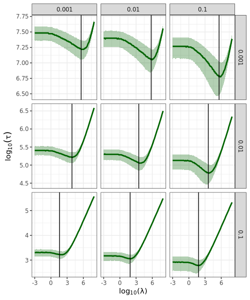
For the purpose of experimentally calibrating λ\lambda as a function of α\alpha and the effect size, we consider a Brownian observation sequence with drift μ\mu, that is we consider St=ψ​t+W⁡(t)S_{t}=\psi t+W(t), ψ≠0\psi\neq 0, with WW a standard Wiener process. We consider various values of ψ\psi and α\alpha and scan through values of λ\lambda. We plot the median, first, and third quartile of the rejection time of the burn-in nmSPRT on the left plot of Fig. 1, and we find and represent the optimal value in the λ\lambda grid for each couple (ψ,α)(\psi,\alpha). We work without a burn-in period, that is we set t0=1t_{0}=1. For the sake of efficiency comparison, also represent the rejection time of the rmlSPRT (which doesn’t depend on OPENλ)\lambda) and the oracle simple-vs-simple SPRT where the numerator corresponds to the (a priori unknown to the analyst) true value of ψ\psi.

Refer to caption
(a) Median, first and third quartiles of burn-in nmSPRT rejection time evaluated at a grid of (α,ψ,λ)(\alpha,\psi,\lambda) values. We run 20000 trajectories of (St)t∈{t1,…,tmax}(S_{t})_{t\in\{t_{1},\ldots,t_{\max}\}} for each triple (α,ψ,λ)(\alpha,\psi,\lambda). Row labels on the right represent α\alpha values, column labels at the top represent μ\mu values. The vertical black line represents the optimal value of λ\lambda for each couple (α,ψ)(\alpha,\psi)
Refer to caption
(b) Optimal λ\lambda for each (α,ψ)(\alpha,\psi). We obtain each point by simulating 20000 trajectories of WtW_{t} for t∈{⌊10i⌋:i∈{0,1/1000⋅1012,2/1000⋅1012,…,1012}}t\in\{\left\lfloor 10^{i}\right\rfloor:i\in\{0,1/1000\cdot 10^{12},2/1000\cdot 10^{12},\ldots,10^{12}\}\} and performing a grid search over values of λ\lambda in {10−3,10−3+0.1,10−3+0.2,…,108}.\{10^{-3},10^{-3+0.1},10^{-3+0.2},\ldots,10^{8}\}. The dashed line corresponds to λ=ψ−2\lambda=\psi^{-2}. The solid lines represent the fit of a local polynomial regression of log10⁡(λo​p​t)\log_{10}(\lambda_{opt}) onto log10⁡ψ−2\log_{10}\psi^{-2} obtained using the loess function of the stats R package.
Figure 1: Empirical calibration on Brownian data of λ\lambda for the normal mixture SPRT without burn-in period.

We plot the results of the grid search for the optimal λ\lambda for each (α,μ)(\alpha,\mu) on the right plot of Fig. 1. The plot seems to indicate, as might be expected from the prior-on-effect-size intuition, that the choice λ=μ−2\lambda=\mu^{-2} is close to optimal, at least for small values of α\alpha.

7.2 A heuristic justification of the optimal choice of λ\lambda

Under a Brownian observation sequence S~​(t)=ψ​t+W​(t)\widetilde{S}(t)=\psi t+W(t), the rejection time τ2\tau_{2} of the nmSPRT (without burn-in, which shouldn’t matter as the discussion would be the essentially the same under t0t_{0} such as ψ​t0→0\psi\sqrt{t_{0}}\to 0, as per our asymptotic regimes) of level α\alpha and parameter λ\lambda satisfies

(ψ​τ2+W⁡(τ2))2τ2+λ−log⁡τ2+λλ=−2​log⁡α.\displaystyle\frac{\left(\psi\tau_{2}+W(\tau_{2})\right)^{2}}{\tau_{2}+\lambda}-\log\frac{\tau_{2}+\lambda}{\lambda}=-2\log\alpha. (58)

As α→0\alpha\to 0, τ2→∞\tau_{2}\to\infty, and therefore, ψ​τ2+W⁡(τ2)∼μ​τ2\psi\tau_{2}+W(\tau_{2})\sim\mu\tau_{2}. Therefore, for small α\alpha, τ2\tau_{2} satisfies approximately

(ψ​τ2)2τ2+λ−log⁡τ2+λλ=−2​log⁡α.\displaystyle\frac{\left(\psi\tau_{2}\right)^{2}}{\tau_{2}+\lambda}-\log\frac{\tau_{2}+\lambda}{\lambda}=-2\log\alpha. (59)

Differentiating the above equation with respect to λ\lambda and using that, at the optimum λ∗\lambda^{*} we have that (∂τ2/∂λ)|λ=λ∗=0(\partial\tau_{2}/\partial\lambda)|_{\lambda=\lambda^{*}}=0, yields that

−ψ2​τ22(τ2+λ∗)2−1τ2+λ∗+1λ∗=0,that isτ2+λ∗τ2=λ∗​ψ2.\displaystyle-\frac{\psi^{2}\tau_{2}^{2}}{(\tau_{2}+\lambda^{*})^{2}}-\frac{1}{\tau_{2}+\lambda^{*}}+\frac{1}{\lambda^{*}}=0,\qquad\text{that is}\qquad\frac{\tau_{2}+\lambda^{*}}{\tau_{2}}=\lambda^{*}\psi^{2}. (60)

Injecting the last equality in (59) yields that

τ2​λ−1−log⁡(τ2​λ−1+1)=−2​log⁡α\displaystyle\tau_{2}\lambda^{-1}-\log(\tau_{2}\lambda^{-1}+1)=-2\log\alpha (61)

which implies that τ2/λ\tau_{2}/\lambda must diverge to infinity as α→0\alpha\to 0. Therefore, as α→0\alpha\to 0, (τ2+λ)/τ2→1(\tau_{2}+\lambda)/\tau_{2}\to 1, and thus from (60), we must have that that λ∗/ψ−2→1\lambda^{*}/\psi^{-2}\to 1.

7.3 A sequential test that adaptively tunes λ\lambda

Given the discussion of the previous two sections, it seems natural to use a test statistic that uses an estimate λ^t\widehat{\lambda}_{t} of ψ−2\psi^{-2} instead of a prespecified value of λ\lambda. In keeping with the design logic of non-anticipating running-estimate SPRT statistics, we propose the following test statistic:

Ytadpt−λ=∑s=1tψ^λ^s−1,s−1​Xs−12​ψ^λ^s−1,s−12,whereλ^t=ψ^0,t−2,\displaystyle Y^{\mathrm{adpt}-\lambda}_{t}=\sum_{s=1}^{t}\widehat{\psi}_{\widehat{\lambda}_{s-1},s-1}X_{s}-\frac{1}{2}\widehat{\psi}_{\widehat{\lambda}_{s-1},s-1}^{2},\qquad\text{where}\qquad\widehat{\lambda}_{t}=\widehat{\psi}_{0,t}^{-2}, (62)

and ψ^λ,t=St/(t+λ)\widehat{\psi}_{\lambda,t}=S_{t}/(t+\lambda), for any t+λ>0t+\lambda>0, and ψ^0,0=0\widehat{\psi}_{0,0}=0, as defined earlier. So as to fully specify a test of level α\alpha, it remains to determine the rejection threshold. We speculate that by enforcing a long enough burn-in period, Ytadpt−λY^{\mathrm{adpt}-\lambda}_{t} will behave similarly to an analogous test statistic

Y~tadpt−λ=∑s=1tψ~λ~s−1,s−1​X~s−12​ψ~λ~s−1,s−12\displaystyle\widetilde{Y}^{\mathrm{adpt}-\lambda}_{t}=\sum_{s=1}^{t}\widetilde{\psi}_{\widetilde{\lambda}_{s-1},s-1}\widetilde{X}_{s}-\frac{1}{2}\widetilde{\psi}_{\widetilde{\lambda}_{s-1},s-1}^{2} (63)

obtained from a sequence (X~t)t≥1(\widetilde{X}_{t})_{t\geq 1} of standard normal i.i.d. observations, and therefore, that the rejection threshold for the latter should yield approximately the same type-I error for the former. That is, for a burn-in period of duration t0t_{0}, we are looking for −log⁡αadpt−λ​(α,t0)-\log\alpha^{\mathrm{adpt}-\lambda}(\alpha,t_{0}) such that

P[supt≥t0Y~tadpt−λ≥−logαadpt−λ(α,t0)]=α,\displaystyle P\left[\sup_{t\geq t_{0}}\widetilde{Y}^{\mathrm{adpt}-\lambda}_{t}\geq-\log\alpha^{\mathrm{adpt}-\lambda}(\alpha,t_{0})\right]=\alpha, (64)

that is

E⁡[P⁡[supt≥t0(Y~tadpt−λ−Y~t0adpt−λ)≥−log⁡αadpt−λ​(α,t0)−Y~t0adpt−λ∣ℱ~t0]]=α.\displaystyle E\left[P\left[\sup_{t\geq t_{0}}\left(\widetilde{Y}^{\mathrm{adpt}-\lambda}_{t}-\widetilde{Y}^{\mathrm{adpt}-\lambda}_{t_{0}}\right)\geq-\log\alpha^{\mathrm{adpt}-\lambda}(\alpha,t_{0})-\widetilde{Y}^{\mathrm{adpt}-\lambda}_{t_{0}}\mid\widetilde{\mathcal{F}}_{t_{0}}\right]\right]=\alpha. (65)

Observing that (exp⁡(Y~tadpt−λ−Y~t0adpt−λ)t≥t0CLOSE(\exp(\widetilde{Y}^{\mathrm{adpt}-\lambda}_{t}-\widetilde{Y}^{\mathrm{adpt}-\lambda}_{t_{0}})_{t\geq t_{0}} is a martingale with initial value 1, we should have, from Ville’s inequality case of equality, that the above equation is approximately equivalent, for t0t_{0} large enough, to

E⁡[exp⁡(−(−log⁡αadpt−λ​(α,t0)−Y~t0adpt−λ)+)]=α.\displaystyle E\left[\exp\left(-\left(-\log\alpha^{\mathrm{adpt}-\lambda}(\alpha,t_{0})-\widetilde{Y}^{\mathrm{adpt}-\lambda}_{t_{0}}\right)_{+}\right)\right]=\alpha. (66)

We propose to solve the above equation by performing a grid search over candidate values of −log⁡αadpt−λ​(α,t0)−Y~t0adpt−λ-\log\alpha^{\mathrm{adpt}-\lambda}(\alpha,t_{0})-\widetilde{Y}^{\mathrm{adpt}-\lambda}_{t_{0}} and evaluating the above expectation at the grid points by Monte-Carlo simulations. (Note that the Monte-Carlo simulation entails drawing multiple trajectories of an i.i.d. sequence (X~t)t≥t0(\widetilde{X}_{t})_{t\geq t_{0}} of standard normal random variables, as opposed to drawing multiple trajectories of the data sequence, which of course is not possible). Our proposed procedure is then the one that starts monitoring the test statistic Ytadpt−λY^{\mathrm{adpt}-\lambda}_{t} after a burn-in period of length t0t_{0} and rejects the null hypothesis as soon as it crosses the rejection threshold −log⁡αadpt−λ​(α,t0)-\log\alpha^{\mathrm{adpt}-\lambda}(\alpha,t_{0}) after t0t_{0}.

We do not analyze formally this procedure in the current version of this work, but we do evaluate it empirically alongside the previously discussed delayed-start nmSPRT and rmlSPRT in the next section.

8 Numerical experiments

We now confirm experimentally the type-I error and expected rejection time guarantees for delayed-start rmlSPRT and nmSPRT confidence sequences, and we compare them to alternative confidence sequences.

8.1 Type-I error

We start with type-I error experiments. We consider a sequence of i.i.d. observations O1,O2,…∼Bernoulli⁡(0.03)−0.03O_{1},O_{2},\ldots\sim\mathrm{Bernoulli}(0.03)-0.03. The choice of the relatively small value 0.030.03 is to ensure that the sum StS_{t} of the stabilized martingale difference X1,X2,…X_{1},X_{2},\ldots sequence doesn’t converge too fast to a normal. It is of course impossible to evaluate the event {τ<∞}\{\tau<\infty\} for any sequential test τ\tau, but, since the martingales we consider must follow the law of the iterated logarithm and the sequences we study have t​log⁡t\sqrt{t\log t} asymptotics, rejections should happen early on. We evaluate boundary crossings at the points of a time grid t1,t2,…,tNt_{1},t_{2},\ldots,t_{N} such that ti≈tmax​∑j=1ijβ/∑j=1Njβt_{i}\approx t_{\max}\sum_{j=1}^{i}j^{\beta}/\sum_{j=1}^{N}j^{\beta}, with N=20000N=20000, β=2\beta=2 and tmax=108t_{\max}=10^{8}. This specification ensures that the time grid is denser early on the time axis. We refer the reader to our code for implementation details.

Refer to caption
(a) Type-I error of the rmle-SPRT sequence, binmSPRT sequence with λ=1\lambda=1 and binmSPRT sequence with λ=100\lambda=100, as a function of the burn-in time t0t_{0}, at levels α∈{5⋅10−3,1⋅10−2,5⋅10−2,1⋅10−1}\alpha\in\{5\cdot 10^{-3},1\cdot 10^{-2},5\cdot 10^{-2},1\cdot 10^{-1}\}. We simulate 5000 trajectories of StS_{t} per point.
Refer to caption
(b) Comparison of type-I error of sequences with burn-in with sequences without burn-in period, namely Howard et al. 2021’s finite sample LIL, given by 1.7​t⁡(log⁡log⁡t+0.72​log⁡(10.4/α))1.7\sqrt{t(\log\log t+0.72\log(10.4/\alpha))}, and the nmSPRT sequences (t+λ)​(2​log⁡α−1+log⁡((t+λ)/λ))\sqrt{(t+\lambda)(2\log\alpha^{-1}+\log((t+\lambda)/\lambda))}, with λ=1\lambda=1 and λ=100\lambda=100. Chosen significance level is α=5⋅10−2\alpha=5\cdot 10^{-2}. Number of simulated trajectories per point is 100000 for sequences with burn-in and 200000 for sequences without burn-in.
Figure 2: Type-I error as a function of t0t_{0}. The confidence bands are 95% pointwise Wald-type confidence sequences. We obtain each point in the above two plots by simulating trajectories of (St,t∈{t1,…,tmax})(S_{t},t\in\{t_{1},\ldots,t_{\max}\}). The dashed black line represents the nominal α\alpha level, of which the value is indicated on the right side of the plots.

Fig. 2 shows convergence of the type-I error with the burn-in period, while the confidence sequences without burn-in period over reject, likely due to erroneous early rejections at time points when StS_{t} is still far from its Wiener process approximations. Note also that for λ=100\lambda=100, we don’t observe over-rejections even for small values of t0t_{0}. This is to be expected as setting λ\lambda trades off early rejections for later tightness. It can be directly observed from the expression of the nmSPRT confidence sequence that the width of the sequence increases early as λ\lambda increases. is also to be expected from the interpretation of λ−1/2\lambda^{-1/2} as a prior on the effect size: if the effect size is of order λ−1/2\lambda^{-1/2} a confidence sequence optimally targeting that effect size should be loose for t≪λt\ll\lambda and tight around λ\lambda, thereby preventing early rejections if λ\lambda is large.

8.2 Rejection time

We now turn to evaluating features of the distribution of the rejection time. As the reader might have noticed, we haven’t discussed in detail so far the choice of the parameter λ\lambda in the nmSPRT expression, beyond the interpretation of λ−1/2\lambda^{-1/2} as an a priori belief on the magnitude of the effect size. We investigate empirically the effect of λ\lambda on the rejection time of the nmSPRT in the next subsection.

We now plot several measures of sample efficiency for the burn-in nmSPRT sequences and the burn-in rmlSPRT sequences. In particular, we plot the ratio of the median stopping time of our tests over the median stopping time of the oracle (in the sense that it uses the true value of μ\mu) simple-vs-simple SPRT with same burn-in period. (We compute the adjusted α\alpha level for the delayed-start simple-vs-simple SPRT in a similar fashion to that of the delayed-start nmSPRT and rmlSPRT). We refer to this ratio as the “relative efficiency” of the sequential tests.

Refer to caption
(a) Relative efficiency as a function of α\alpha for various values of μ\mu. The panel labels at the top represent the values of α\alpha.
Refer to caption
(b) Relative efficiency as a function of μ\mu, for various values of α\alpha. The panel labels at the top represent the values of α\alpha
Figure 3: Relative efficiency, defined as median⁡(τ)/median⁡(τsvs)\mathrm{median}(\tau)/\mathrm{median}(\tau^{\mathrm{svs}}). We obtain each point by simulating 8000 trajectories of (St)t∈{t1,…,tmax}(S_{t})_{t\in\{t_{1},\ldots,t_{\max}\}}, for i.i.d. observations O1,O2​…,∼μ+(Bernoulli⁡(0.03)−0.03)O_{1},O_{2}\ldots,\sim\mu+(\mathrm{Bernoulli}(0.03)-0.03).

We observe on the left subplot of Fig. 3 that the relative efficiency of the (delayed-start) rmlSPRT and the nmSPRT seem to converge to 1 as α→0\alpha\to 0, as implied by Theorem 4. An empirical (as opposed to predicted by any of the theorems of the current article) finding we infer from the right plot of Fig. 3 is that the median stopping time of the nmSPRT at the optimal λ\lambda value seems to be within a constant factor c⁡(α)>1c(\alpha)>1 of the median stopping time of the oracle simple-vs-simple SPRT, and that c⁡(α)→1c(\alpha)\to 1 as α→0\alpha\to 0.

Refer to caption
Figure 4: Median, first and third quartile of the ratio of the rejection time with the asymptotic upper bound 2​μ−2​log⁡μ−12\mu^{-2}\log\mu^{-1} from Theorem 4, for the burn-in oracle simple-vs-simple SPRT, burn-in nmSPRT, burn-in rmlSPRT, and burn-in nmSPRT with adaptive λ\lambda. We obtain each point by simulating 8000 trajectories of (St)t∈{t1,…,tmax}(S_{t})_{t\in\{t_{1},\ldots,t_{\max}\}}, for i.i.d. observations O1,O2​…∼μ+(Bernoulli⁡(0.03)−0.03)O_{1},O_{2}\ldots\sim\mu+(\mathrm{Bernoulli}(0.03)-0.03). We set α=5⋅10−2\alpha=5\cdot 10^{-2} for the current plot. We set the burn-in period t0t_{0} to 200. The panel labels at the top represent the value of α\alpha.

9 Application to quality-control of Netflix client application

We illustrate the use of the delayed-start rmlSPRT and of the delayed-start nmSPRT on a real data case study. We also compare it to an empirical Bernstein sequential boundary based on a gamma-exponential mixture boundary, as proposed in section 4 of (Howard et al. 2021).

Our data comes from an A/B test used to quality-control the release of a new Netflix client application. Users in the treatment and control groups experienced new and existing versions of the Netflix software respectively. The outcome of interest was the delay between requesting playback and the stream starting, which we term “play delay”. Although this dataset was collected according to a pre-determined sample size, we use it to illustrate the performance of our sequential tests. In the following, pre-treatment measurements of play delay are available for all experimental units, which are leveraged for regression adjustment. We work with log-transformed play delay, and use an undisclosed base to protect proprietary information.

We simulate observation trajectories (Xt)t≥1(X_{t})_{t\geq 1} as follows: for each tt, we draw uniformly at random treatment assignment At∈{0,1}A_{t}\in\{0,1\} and then we draw outcome UtU_{t} and a pre-treatment covariate LtL_{t} by sampling with replacement from actual realized pairs (L,U)(L,U) in arm AtA_{t} in the test data. The data structure is an instance of a Bernoulli trial with covariates as described in the second example at the beginning of the article. The outcome UtU_{t} is, as we mentioned, the play delay. We use as covariate LtL_{t} the pre-treatment outcome of unit tt, that is the play-delay before treatment assignment. The probability of assignment to cell 1 is p=0.5p=0.5. Our null hypothesis is that there is no difference in play delay on average between the newer and existing Netflix client, that is H0:θ=0H_{0}:\theta=0, where θ=E⁡[U1∣A1=1]−E⁡[U1∣A1=0]\theta=E[U_{1}\mid A_{1}=1]-E[U_{1}\mid A_{1}=0] identifies this mean causal effect. As in our Bernoulli trial with covariates example, we let

Zt=η^t−1​(1,Lt)−η^t−1​(0,Lt)+At−pp⁡(1−p)​(Ut−η^t−1​(At,Lt)),\displaystyle Z_{t}=\widehat{\eta}_{t-1}(1,L_{t})-\widehat{\eta}_{t-1}(0,L_{t})+\frac{A_{t}-p}{p(1-p)}(U_{t}-\widehat{\eta}_{t-1}(A_{t},L_{t})), (67)

where ηt−1​(a,l)\eta_{t-1}(a,l) is a least-squares estimator of the linear regression of UU on LL, L×AL\times A and an intercept, computed from observations indexed by ℐ1,t\mathcal{I}_{1,t}, where the index set ℐ1,t\mathcal{I}_{1,t} is as introduced in section 6. We set Xt=σ^t−1−1​ZtX_{t}=\widehat{\sigma}_{t-1}^{-1}Z_{t} where σ^t−1\widehat{\sigma}_{t-1} is a 𝒟0,t\mathcal{D}_{0,t}-measurable estimator of the standard deviation of ZtZ_{t}.

We set the burn-in period t0t_{0} to 1000 observations and the normal mixture SPRT tuning parameter λ\lambda to 10210^{2}. Measurements of play delay are bounded from above by bb, as longer delays are simply abandoned. When using the empirical Bernstein boundary (Howard et al. 2021), ηt−1​(a,l)\eta_{t-1}(a,l) is the same linear predictor projected onto the interval [0,b][0,b], ensuring Zt∈[−2​b,2​b]Z_{t}\in[-2b,2b]. In their notation, we use a scale c=4​bc=4b, and a gamma-exponential mixture with parameter ρ\rho. Following the recommendation formulated in their section 3.5, we set the gamma-exponential mixture parameter ρ\rho to the same as the Gaussian mixture parameter λ=100\lambda=100. We make these choices based on domain knowledge of these types of experiments. They correspond to a target effect size of the order of 11%, and to the fact that we typically get a hundredfold gain in sample size from pre-allocation outcome adjustment. While in the context of our simulation we of course know the effect size (it turns out the point estimate is -0.81%) since we work from an already fully collected data set, the 11% order of magnitude is what engineers at Netflix expect using domain specific expertise.

So as to make things more concrete, we plot in figure 5 the trajectory of the test statistics for one arbitrary random draw of the data sequence. We see that if we had received the data in the particular order of the simulated stream, we would have called the test after collecting slightly after the end of the burn-in period t0=1000t_{0}=1000 while the non-asymptotic empirical Bernstein test stops at almost 10410^{4} observations.

We now examine the behavior of the test statistics over many draws of the data sequence. We first examine the empirical Type-I error of the nmSPRT by simulating data under the null hypothesis. Specifically, we simulate data for both treatment and control by sampling with replacement from observed control dataset, which we refer to as a simulated A/A test. Figure 6, left, shows that the Type-I error approaches the nominal 5% the longer the simulation is performed.

We then compare the behavior of the rmlSPRT, the nmSPRT and the non-asymptotic empirical Bernstein test on simulated trajectories of the A/B test (unlike in the A/A test, here observations for treatment and control units are drawn from their respective empirical distributions obtained from the observed dataset, following simulated treatment assignment AtA_{t}). We plot simulation results in figure 6. In this example, the rmlSPRT and the nmSPRT perform relatively similary due to the fact that we chose λ\lambda in the normal mixture to optimize for rejection times of the order of 10210^{2}, which is earlier than the end of the burn-in time. As expected, the empirical Bernstein test is much more conservative, and we observe it tends to reject a little less than an order of magnitude later.

Refer to caption
Figure 5: nmSPRT and rMLE test statistics trajectories on one arbitrary draw of the data sequence in the play delay case study.
Refer to caption
(a) Empirical CDFs of the rejection times of the three sequential tests for 1000 simulated trajectories of the A/A experiment.
Refer to caption
(b) Empirical CDFs of the rejection times of the three sequential tests for 1000 simulated trajectories of the A/B experiment.
Figure 6: Behavior of the rejection time of the mixture SPRT, running-maximum-likelihood SPRT, and the empirical Bernstein sequential test under simulated A/A experiments and simulated A/B experiments in the play delay case study.

10 From Wald’s simple-vs-simple SPRT to delayed-start running-mean-estimate SPRTs

In this section, we expose the historical and logical progression from Wald’s results (Wald 1945; Wald 1947; Wald and Wolfowitz 1948; Wald and Wolfowitz 1950) on the optimality of simple-vs-simple parametric SPRTs to our results, that is the type-I error calibration and expected rejection time optimality of the non-parametric delayed-start running-mean-estimate.

10.1 Type-I error and optimality of the oracle simple-vs-simple SPRT

Definition and type-I error.

Wald 1945; Wald 1947 introduced the sequential probability ratio test, defined as follows. Suppose that X1,X2,…X_{1},X_{2},\ldots are i.i.d. drawn from a common distribution with density pp w.r.t a certain measure. Consider two simple hypotheses H0:p=p0H_{0}:p=p_{0} and H1:p=p1H_{1}:p=p_{1}, with p1/p0<∞p_{1}/p_{0}<\infty. The SPRT statistic at tt is the likelihood ratio

Ytsvs=∏s=1tp1​(Xt)p0​(Xt),\displaystyle Y^{\mathrm{svs}}_{t}=\prod_{s=1}^{t}\frac{p_{1}(X_{t})}{p_{0}(X_{t})}, (68)

and the α\alpha-level SPRT is the stopping time τsvs=inf{t≥1:Ytsvs≥−log⁡α}\tau^{\mathrm{svs}}=\inf\{t\geq 1:Y^{\mathrm{svs}}_{t}\geq-\log\alpha\}. That type-I error is at most α\alpha follows, via Ville’s inequality (Ville 1939), from the fact that (Ytsvs)t≥1(Y_{t}^{\mathrm{svs}})_{t\geq 1} is a martingale under H0H_{0} with initial value 1.

Power, expected rejection time.

Wald 1945; Wald 1947 shows that the SPRT has power 1 under the alternative H1H_{1} and that its expected rejection time as dK​L​(p1,p0)→0d_{KL}(p_{1},p_{0})\to 0 is asymptotically equivalent to −logα/dK​L(p,p0)-\log\alpha/d_{KL}(p_{,}p_{0}), where dK​Ld_{KL} is the Kullback-Leibler divergence. Wald and Wolfowitz 1948 further show that, under the present setting, the expected stopping time of the simple-vs-simple SPRT is optimal among all tests of level α\alpha under H0H_{0}, that is, for any sequential test τ′\tau^{\prime} such that PrH0[τ′<∞]≤α\mathrm{Pr}_{H_{0}}[\tau^{\prime}<\infty]\leq\alpha, we must have EH1​[τ′]≥EH1​[τsvs]E_{H_{1}}[\tau^{\prime}]\geq E_{H_{1}}[\tau^{\mathrm{svs}}].

10.2 Mixture SPRTs for the Wiener process and for parametric sequence of i.i.d. random variables

The case for mixture test statistics under composite alternatives.

Consider a family of densities pψp_{\psi} indexed by a one-dimensional parameter ψ\psi and the null hypothesis H0:ψ=ψ0H_{0}:\psi=\psi_{0}. It is often the case that the alternative hypothesis is a composite alternative of the form H\0=ψ≠ψ0H_{\backslash 0}=\psi\neq\psi_{0}. In clinical trials or A/B tests for instance, experimenters want to test the absence of average treatment effect (ATE) against the hypothesis that the ATE is non-zero, rather than against a specific non-zero value of the ATE.

It can be shown that for p∈H\0p\in H_{\backslash 0} such that pp is closer in Kullback-Leibler divergence to H0H_{0} than it is to H1H_{1}, the simple-vs-simple SPRT of H0H_{0} against H1H_{1} has power strictly smaller than 1. It can further be shown that, even if dKL​(p,H1)<dKL​(p,H0)d_{\mathrm{KL}}(p,H_{1})<d_{\mathrm{KL}}(p,H_{0}), the expected stopping time can get highly suboptimal as ψ\psi gets away from ψ1\psi_{1}.

A remedy to this limitation of the simple-vs-simple SPRT that ensures the resulting sequential test has power 1 against any ψ1≠ψ0\psi_{1}\neq\psi_{0}, is to use a prior FF over the possible values of ψ1\psi_{1}. This yields so-called mixture SPRTs, introduced by Robbins and Siegmund 1970; Robbins 1970, where FF is the so-called mixture distribution, in which the test statistic and the test are defined as

Ytmixt=∫∏s=1tpψ1​(Xt)pψ0​(Xt)​𝑑F​(ψ1)andτmixt=inf{t≥1:Ytmixt≥−log⁡α}.\displaystyle Y^{\mathrm{mixt}}_{t}=\int\prod_{s=1}^{t}\frac{p_{\psi_{1}}(X_{t})}{p_{\psi_{0}}(X_{t})}dF(\psi_{1})\qquad\text{and}\qquad\tau^{\mathrm{mixt}}=\inf\{t\geq 1:Y^{\mathrm{mixt}}_{t}\geq-\log\alpha\}. (69)

Integrating against FF preserves the martingale property under H0H_{0} and therefore the type-I error guarantee.

Mixture confidence sequences for normal data.

Under an i.i.d. sequence X1,X2​…∼𝒩⁡(ψ,1)X_{1},X_{2}\ldots\sim\mathcal{N}(\psi,1), that is under pψ(x)=(2π)−1/2exp(−(x−ψ)2/2)p_{\psi}(x)=(2\pi)^{-1/2}\exp(-(x-\psi)^{2}/2), YtmixtY_{t}^{\mathrm{mixt}} takes the form

Ytmixt=∫exp⁡((ψ1−ψ0)​St−12​(ψ1−ψ0)2​t)​𝑑F​(ψ1)whereSt=∑s=1tXs.\displaystyle Y_{t}^{\mathrm{mixt}}=\int\exp\left((\psi_{1}-\psi_{0})S_{t}-\frac{1}{2}(\psi_{1}-\psi_{0})^{2}t\right)dF(\psi_{1})\qquad\text{where}\qquad S_{t}=\sum_{s=1}^{t}X_{s}. (70)

It is common to specify the null hypothesis by setting ψ0=0\psi_{0}=0 (think about testing the absence of average treatment effect against non-zero ATE). An analytically convenient mixture distribution FF is the normal distribution (Robbins and Siegmund 1970; Robbins 1970) centered around 0 and with variance λ−1\lambda^{-1}. The variance of the mixture distribution encodes beliefs about the possible values of the effect size if it isn’t zero. This yields

Ytmixt=λt+λ​exp⁡(12​St2t+λ).\displaystyle Y_{t}^{\mathrm{mixt}}=\sqrt{\frac{\lambda}{t+\lambda}}\exp\left(\frac{1}{2}\frac{S_{t}^{2}}{t+\lambda}\right). (71)

Inverting YtmixtY_{t}^{\mathrm{mixt}} yields a confidence sequence for StS_{t}. Specifically, for any α>0\alpha>0, that PrH0[τmixt<∞]≤α\Pr_{H_{0}}[\tau^{\mathrm{mixt}}<\infty]\leq\alpha is equivalent to the fact that

|St|≤(t+λ)​(−2​log⁡α+log⁡(t+λλ))∀t≥1.\displaystyle|S_{t}|\leq\sqrt{(t+\lambda)\left(-2\log\alpha+\log\left(\frac{t+\lambda}{\lambda}\right)\right)}\qquad\forall t\geq 1. (72)
Exact calibration for Wiener processes.

Robbins and Siegmund 1970 further show that for a standard Wiener process, the crossing probability of boundary (72) is exactly α\alpha, while it is only known that it is at most α\alpha in the case of discrete normal i.i.d. data.

10.3 Running-estimate SPRTs

Definition of the running-estimate SPRTs.

A seemingly different strategy to modify the simple-vs-simple SPRT so as to obtain a test of power one against composite alternatives is to harness the sequentiality of data collection by using likelihood ratios of the form Ytrngest=∏s=1tpψ^s−1​(Xt)/pψ0​(Xt)Y^{\mathrm{rngest}}_{t}=\prod_{s=1}^{t}p_{\widehat{\psi}_{s-1}}(X_{t})/p_{\psi_{0}}(X_{t}), where ψ^s−1\widehat{\psi}_{s-1} is a running ℱs−1\mathcal{F}_{s-1}-measurable estimate of ψ\psi. This is the approach proposed by Robbins and Siegmund 1972 to design one-sided tests of H≤ψ0:ψ≤ψ0H_{\leq\psi_{0}}:\psi\leq\psi_{0} against H>ψ0:ψ>ψ0H_{>\psi_{0}}:\psi>\psi_{0}. A running estimate used by Robbins and Siegmund 1972 in the case of a sequence of i.i.d data drawn from 𝒩⁡(ψ,1)\mathcal{N}(\psi,1) is the threhsolded maximum likelihood estimator (MLE) ψ^t=t−1​(∑s=1tXs−ψ0)++ψ0\widehat{\psi}_{t}=t^{-1}(\sum_{s=1}^{t}X_{s}-\psi_{0})_{+}+\psi_{0}, while another one is the posterior mean computed from X1,…,XtX_{1},\ldots,X_{t}, under a prior FF with support [ψ0,∞)[\psi_{0},\infty).

Optimality.

It makes sense that the running-estimate SPRTs should have close to optimal expected rejection time, as ψ~s−1\widetilde{\psi}_{s-1} is a proxy for ψ\psi, and we know from Wald and Wolfowitz 1948 that the level-α\alpha-under-H0H_{0} test with optimal rejection time under ψ=ψ1\psi=\psi_{1} is the simple-vs-simple SPRT of H0H_{0} against H1H_{1}. Robbins and Siegmund 1974 study the expected rejection time of one-sided tests of H≤ψ0H_{\leq\psi_{0}} against H>ψ0H_{>\psi_{0}} of the form τrngest=inf{t≥1:Ytrngest≥−log⁡α}\tau^{\mathrm{rngest}}=\inf\{t\geq 1:Y^{\mathrm{rngest}}_{t}\geq-\log\alpha\} as ψ↓ψ0\psi\downarrow\psi_{0}. They prove that when ψ^t\widehat{\psi}_{t} is taken to be the thresholded MLE, E[τrngest]∼PH0[τrngest=∞](ψ−ψ0)−2log(ψ−ψ0)−1E[\tau^{\mathrm{rngest}}]\sim P_{H_{0}}[\tau^{\mathrm{rngest}}=\infty](\psi-\psi_{0})^{-2}\log(\psi-\psi_{0})^{-1}. This isn’t too far off the lower bound 2PH0[τrngest=∞](ψ−ψ0)−2loglog(ψ−ψ0)−12P_{H_{0}}[\tau^{\mathrm{rngest}}=\infty](\psi-\psi_{0})^{-2}\log\log(\psi-\psi_{0})^{-1} proven by Farrell 1964 for such one-sided tests as ψ↓ψ0\psi\downarrow\psi_{0}.

Connection to mixture SPRTs and confidence sequences.

Robbins and Siegmund 1974 show that the running-estimate SPRTs exhibit an interesting connection to mixture SPRTs in the case where the data stream is a time-continuous process of the form (S~​(t))t≥0(\widetilde{S}(t))_{t\geq 0}, with S~​(t)=ψ​t+W​(t)\widetilde{S}(t)=\psi t+W(t) for all t≥0t\geq 0, where (W⁡(t))t≥0(W(t))_{t\geq 0} is a standard Wiener process. We expose their observations here. Denote 𝔉~=(ℱ~​(t))t≥0\widetilde{\mathfrak{F}}=(\widetilde{\mathcal{F}}(t))_{t\geq 0} the canonical filtration to which WW is adapted. The Brownian continuous-time analog of the class of test statistics of the form YtrngestY_{t}^{\mathrm{rngest}} is the class of test statistics of the form:

Y~trngest=exp⁡(∫0tψ~​(s)​𝑑S~​(s)−12​ψ~​(s)2​𝑑s),\displaystyle\widetilde{Y}^{\mathrm{rngest}}_{t}=\exp\left(\int_{0}^{t}\widetilde{\psi}(s)d\widetilde{S}(s)-\frac{1}{2}\widetilde{\psi}(s)^{2}ds\right), (73)

where ψ~​(s)\widetilde{\psi}(s) is an ℱ~s\widetilde{\mathcal{F}}_{s}-measurable estimate of ψ\psi. Meanwhile, Brownian continuous-time mixture test statistics take the form

Y~tmixt=f⁡(S~t,t)wheref⁡(x,t)=∫exp⁡(ψ′​x−12​ψ′2​t)​𝑑F​(ψ′),\displaystyle\widetilde{Y}_{t}^{\mathrm{mixt}}=f(\widetilde{S}_{t},t)\qquad\text{where}\qquad f(x,t)=\int\exp\left(\psi^{\prime}x-\frac{1}{2}\psi^{\prime 2}t\right)dF(\psi^{\prime}), (74)

where FF is the mixing distribution. Itô’s lemma asserts that for any stochastic process (X⁡(t))t≥0(X(t))_{t\geq 0} of the form X⁡(t)=X⁡(0)+∫0tμ⁡(s)​𝑑s+σ⁡(s)​𝑑W​(s)X(t)=X(0)+\int_{0}^{t}\mu(s)ds+\sigma(s)dW(s), where σ⁡(s)\sigma(s) and μ⁡(s)\mu(s) are ℱ~​(s)\widetilde{\mathcal{F}}(s)-measurable, and any suitably differentiable (x,t)↦u⁡(x,t)(x,t)\mapsto u(x,t), it holds that u⁡(Xt,t)=u⁡(0,0)+∫0t∂xu⁡(Xs,s)​𝑑X​(s)+(∂tu⁡(Xs,s)+12​∂x,xu⁡(Xs,s))​𝑑su(X_{t},t)=u(0,0)+\int_{0}^{t}\partial_{x}u(X_{s},s)dX(s)+(\partial_{t}u(X_{s},s)+\frac{1}{2}\partial_{x,x}u(X_{s},s))ds. Applying Itô’s lemma to u⁡(S~​(t),t)=log⁡f⁡(S~​(t),t)u(\widetilde{S}(t),t)=\log f(\widetilde{S}(t),t) yields

Y~tmixt=exp⁡(∫0tψ~′​(s)​𝑑S~​(s)−12​(ψ~′​(s))2​𝑑s)whereψ~′​(s)=∂xff​(S~​(s),s).\displaystyle\widetilde{Y}^{\mathrm{mixt}}_{t}=\exp\left(\int_{0}^{t}\widetilde{\psi}^{\prime}(s)d\widetilde{S}(s)-\frac{1}{2}\left(\widetilde{\psi}^{\prime}(s)\right)^{2}ds\right)\qquad\text{where}\qquad\widetilde{\psi}^{\prime}(s)=\frac{\partial_{x}f}{f}(\widetilde{S}(s),s). (75)

Notice that

ψ~′​(s)=∫ψ′​exp⁡(ψ′​S~​(s)−12​ψ′2​t)​d​F​(ψ′)∫exp⁡(ψ′​S~​(s)−12​ψ′2​t)​𝑑F​(ψ′)\displaystyle\widetilde{\psi}^{\prime}(s)=\int\psi^{\prime}\frac{\exp(\psi^{\prime}\widetilde{S}(s)-\frac{1}{2}\psi^{\prime 2}t)dF(\psi^{\prime})}{\int\exp(\psi^{\prime}\widetilde{S}(s)-\frac{1}{2}\psi^{\prime 2}t)dF(\psi^{\prime})} (76)

is the posterior mean of ψ\psi given ℱ~​(s)\widetilde{\mathcal{F}}(s) under prior FF. For F=𝒩⁡(0,λ−1)F=\mathcal{N}(0,\lambda^{-1}), we have that ψ~′​(s)=S~​(s)/(s+λ)\widetilde{\psi}^{\prime}(s)=\widetilde{S}(s)/(s+\lambda), that is the shrunken empirical mean with shrinkage parameter λ\lambda. This shows in particular that the normal mixture boundary (72) is equivalent to Y~trngest≤−log⁡α\widetilde{Y}^{\mathrm{rngest}}_{t}\leq-\log\alpha with ψ~​(s)=ψ~′​(s)=S~​(s)/(s+λ)\widetilde{\psi}(s)=\widetilde{\psi}^{\prime}(s)=\widetilde{S}(s)/(s+\lambda). Robbins and Siegmund 1974 show in their Theorem 3 that in the normal discrete case, the half-normal prior yields a running-posterior-mean SPRT with expected rejection time behaving as 2PH0[τrngest=∞](ψ−ψ0)−2log(ψ−ψ0)−12P_{H_{0}}[\tau^{\mathrm{rngest}}=\infty](\psi-\psi_{0})^{-2}\log(\psi-\psi_{0})^{-1}.

Boundary associated to the running MLE SPRT

As far as we are aware, there doesn’t seem to be a mixture distribution corresponding to the MLE or to the thresholded MLE alluded to earlier. However, application of Itô’s lemma to h⁡(x,t)=x2/(2​t)h(x,t)=x^{2}/(2t) yields that the running MLE SPRT log test statistic started at 1 can be rewritten as follows:

log⁡YtrmlSPRT=\displaystyle\log Y^{\mathrm{rmlSPRT}}_{t}= ∫1tS~​(s)s​𝑑S~​(s)−12​(S~​(s)s)2​𝑑s\displaystyle\int_{1}^{t}\frac{\widetilde{S}(s)}{s}d\widetilde{S}(s)-\frac{1}{2}\left(\frac{\widetilde{S}(s)}{s}\right)^{2}ds (77)
=\displaystyle= ∫1td​h​(S~​(s),s)−12​s​𝑑s=12​(S~​(t)2s−S~​(1)2−log⁡t).\displaystyle\int_{1}^{t}dh(\widetilde{S}(s),s)-\frac{1}{2s}ds=\frac{1}{2}\left(\frac{\widetilde{S}(t)^{2}}{s}-\widetilde{S}(1)^{2}-\log t\right). (78)

Under the null H0H_{0}, (YtrmlSPRT)t≥1(Y_{t}^{\mathrm{rmlSPRT}})_{t\geq 1} is a martingale with initial value 1. Therefore, from Ville’s inequality,

Pr[12(W​(t)2t−logt)≥x]\displaystyle\Pr\left[\frac{1}{2}\left(\frac{W(t)^{2}}{t}-\log t\right)\geq x\right] (79)
=\displaystyle= E⁡[Pr⁡[12​(W​(t)2t−W​(1)2−log⁡t)≥x−12​W​(1)2∣W⁡(1)]]\displaystyle E\left[\Pr\left[\frac{1}{2}\left(\frac{W(t)^{2}}{t}-W(1)^{2}-\log t\right)\geq x-\frac{1}{2}W(1)^{2}\mid W(1)\right]\right] (80)
=\displaystyle= E⁡[exp⁡((−x+12​W​(1)2)+)].\displaystyle E\left[\exp\left(\left(-x+\frac{1}{2}W(1)^{2}\right)_{+}\right)\right]. (81)

It can readily be checked that putting x=−log⁡α~1​(α)x=-\log\widetilde{\alpha}_{1}(\alpha) sets the above quantity to α\alpha. Therefore, inverting YtrmlSPRTY^{\mathrm{rmlSPRT}}_{t} gives that, with probability 1−α1-\alpha,

|W⁡(t)|≤t⁡(−2​log⁡α~1​(α)+log⁡t),∀t≥1.\displaystyle|W(t)|\leq\sqrt{t\left(-2\log\widetilde{\alpha}_{1}(\alpha)+\log t\right)},\qquad\forall t\geq 1. (82)

10.4 Toward non-parametricity: delayed start mixture SPRTs under i.i.d. data

Theorem 2 in Robbins and Siegmund 1970 asserts (we present here a slight two-sided modification of the result) that for a sequence X1,X2,…X_{1},X_{2},\ldots of i.i.d. random variables with mean 0 and variance 1, and a boundary function (c⁡(u))u≥u0(c(u))_{u\geq u_{0}} such that (i) c(u)u−1/2c(u)u^{-1/2} is non-decreasing for uu large enough and (ii) ∫u0∞u−3/2c(u)exp(−c(u)2/2)du<∞\int_{u_{0}}^{\infty}u^{-3/2}c(u)\exp(-c(u)^{2}/2)du<\infty, it holds that

limt0→∞P[∀t∈ℕ∩[u0t0,∞),|St|≤t0c(t/t0)]=P[∀u≥u0,|W(u)|≤c(u)].\displaystyle\lim_{t_{0}\to\infty}P\left[\forall t\in\mathbb{N}\cap[u_{0}t_{0},\infty),|S_{t}|\leq\sqrt{t_{0}}c(t/t_{0})\right]=P\left[\forall u\geq u_{0},|W(u)|\leq c(u)\right]. (83)

This result therefore allows, in nonparametric i.i.d. settings, to obtain approximate confidence sequences from a confidence sequence for the Wiener process, by means of a burn-in period and a time-rescaling. Applying this result to (72) and (82) yields that

limt0→∞\displaystyle\lim_{t_{0}\to\infty} Pr[∀t∈ℕ∩[t0,∞),|St|≤(t+η​t0)​(−2​log⁡α~2,η​(α)+log⁡t+η​t0η​t0)]\displaystyle\Pr\left[\forall t\in\mathbb{N}\cap[t_{0},\infty),\ |S_{t}|\leq\sqrt{(t+\eta t_{0})\left(-2\log\widetilde{\alpha}_{2,\eta}(\alpha)+\log\frac{t+\eta t_{0}}{\eta t_{0}}\right)}\right] (84)
=\displaystyle= Pr[∀u≥1,|W(u)|≤(u+η)​(−2​log⁡α~2,η​(α)+log⁡u+ηη)]\displaystyle\Pr\left[\forall u\geq 1,|W(u)|\leq\sqrt{(u+\eta)\left(-2\log\widetilde{\alpha}_{2,\eta}(\alpha)+\log\frac{u+\eta}{\eta}\right)}\right] (85)

and

limt0→∞\displaystyle\lim_{t_{0}\to\infty} Pr[∀t∈ℕ∩[t0,∞),|St|≤t⁡(−2​log⁡α~1​(α)+log⁡tt0)]\displaystyle\Pr\left[\forall t\in\mathbb{N}\cap[t_{0},\infty),\ |S_{t}|\leq\sqrt{t\left(-2\log\widetilde{\alpha}_{1}(\alpha)+\log\frac{t}{t_{0}}\right)}\right] (86)
=\displaystyle= Pr[∀u≥1,|W(u)|≤u⁡(−2​log⁡α~1​(α)+log⁡u)].\displaystyle\Pr\left[\forall u\geq 1,|W(u)|\leq\sqrt{u\left(-2\log\widetilde{\alpha}_{1}(\alpha)+\log u\right)}\right]. (87)

The key enabling result in the proof of theorem 2 in Robbins and Siegmund 1970 is Donsker’s weak invariance principle for i.i.d. random variables.

10.5 Modern invariance principle based CSs

Weak invariance principle for sequential testing and confidence sequences.

Theorem 10 in Bibaut et al. 2021c uses McLeish 1974’s weak invariance principle for martingale-difference triangular arrays to provide a method for constructing non-parametric asymptotic confidence sequences from a confidence sequence for the Wiener process. We present the result here in the case that X1,X2,…X_{1},X_{2},\ldots is an 𝔉\mathfrak{F}-adapted sequence with Var⁡(Xt∣ℱt−1)=1\mathrm{Var}(X_{t}\mid\mathcal{F}_{t-1})=1, ψt=E⁡[Xt∣ℱt−1]\psi_{t}=E[X_{t}\mid\mathcal{F}_{t-1}] and H0:ψt=0​∀t≥1H_{0}:\psi_{t}=0\ \forall t\geq 1, that is (Xt)(X_{t}) is a martingale difference sequence.

Let u0∈[0,1]u_{0}\in[0,1] and et (c⁡(u))u∈[u0,1](c(u))_{u\in[u_{0},1]} be a symmetric (1−α)(1-\alpha)-confidence sequence for the Wiener process on [u0,1][u_{0},1], that is Pr[∀u∈[u0,1],|W(u)|≤c(u)]≥1−α\Pr[\forall u\in[u_{0},1],|W(u)|\leq c(u)]\geq 1-\alpha. As a relatively direct corollary of theorem 3.2 in McLeish 1974, it holds that

limT→∞Pr[∀t∈ℕ∩[u0T,T]|St|≤Tc(t/T)]=α.\displaystyle\lim_{T\to\infty}\Pr\left[\forall t\in\mathbb{N}\cap[u_{0}T,T]|S_{t}|\leq\sqrt{T}c(t/T)\right]=\alpha. (88)

Here TT plays the role of the maximum runtime of the experiment, while u0u_{0} is the fraction of TT the experimenter uses as burn-in time. The need for TT is a theoretical limitation, although it might not be a practical one, as experimenters generally have a time budget or sample size budget to spend on a trial. In the case of a martingale data sequence, we conjecture that concentration-inequality-based methods similar to the ones used to prove theorem 2 from Robbins and Siegmund 1970 could be used to show limT→∞Pr[∀t∈ℕ∩(T,∞),|St|≤Tc(t/T)]=0\lim_{T\to\infty}\Pr[\forall t\in\mathbb{N}\cap(T,\infty),\ |S_{t}|\leq\sqrt{T}c(t/T)]=0, and therefore get rid of the need for a maximum experiment runtime. However, doing so might be more complex in the originally intended martingale-difference array setting.

Strong invariance principle for asymptotic time-uniform confidence sequences.

Waudby-Smith et al. 2021 introduce the use of strong invariance principles (also known as almost sure invariance principles or strong approximation results) to construct confidence sequences in nonparametric settings. One key contribution of their work is to introduce a definition of asymptotic confidence sequence (AsympCS). They say that a sequence (ct)t∈ℕ(c_{t})_{t\in\mathbb{N}} is a symmetric (1−α)(1-\alpha)-asymptotic confidence sequence for the partial sum process (St)t∈ℕ(S_{t})_{t\in\mathbb{N}} if there exists a (1−α)(1-\alpha)-exact confidence sequence (ct∗)t∈ℕ(c_{t}^{*})_{t\in\mathbb{N}} for (St)t∈ℕ(S_{t})_{t\in\mathbb{N}} such that ct/ct∗→1c_{t}/c^{*}_{t}\rightarrow 1 almost surely.

Successive versions of this article use different strong approximation results. Starting from version 5, they have been using Strassen 1967’s strong invariance principle for martingales and allows for asymptotic confidence sequences for the general setting where (St)t∈ℕ(S_{t})_{t\in\mathbb{N}} is a martingale. Starting from version 7, they also include type I guarantees for sequences of delayed start confidence sequences. Specifically, they replicate with their techniques (and lift some assumptions for) the type-I error guarantee for sequences of delayed-start normal-mixture sequences, initially proven under martingale data in version 1 of the current paper. They also extend the guarantee (87) for sequences of the delayed-start running MLE SPRT sequence to martingale data.

In our view, the main focus of Waudby-Smith et al. 2021 is proposing a novel definition of AsympCS that is asymptotically close in parameter space to an exact 1−α1-\alpha confidence sequence for the parameter of interest. Meanwhile, our work focuses on the testing properties, that is, type-I error and expected rejection time, of sequences of confidence sequences or of tests. In particular, the current version of their paper, version 7 at the time of writing of this work, does not provide a rejection time analysis. One difference between our setting and theirs is that we impose the normalization condition of the conditional variance, which they don’t. We use this condition heavily in our rejection time analysis. We leave to future work the discussion of whether this condition is actually necessary for a rejection time analysis.

11 Related Literature

Classical approaches to hypothesis testing have predominantly dealt with experiments of fixed, predetermined sample sizes, which we refer to as the fixed-n kind. The emphasis on fixed-n tests by early pioneers such as Fisher is presumably a consequence of the motivating applications that drove the development of hypothesis testing procedures in the first half 19th century, in which outcomes of an experiment were only available long after the experiment had been designed, such as in agricultural research (Armitage 1993). As tests could only be performed once, fixed-n tests were designed to maximize power subject to a type-I error constraint (Neyman et al. 1933). Increasingly in modern experiments, however, observations from experimental units become available sequentially instead of simultaneously, providing many opportunities to perform a test instead of just one. The application of fixed-n tests to sequential designs is made difficult because it requires making an undesirable trade-off balancing the competing objectives of detecting large effects early and detecting small effects eventually. Performing the test later risks exposing many experimental units to a potentially large and harmful treatment effect, while performing the test early risks a high type-II error for small effects. These desires have led to bad statistical practices whereby fixed-n procedures are naively applied to accumulating sets of data, see Johari et al. 2017 for a discussion pertaining to online A/B tests, which sacrifice type-I error guarantees (Armitage et al. 1969), permitting the analyst to incorrectly sample to a foregone conclusion (Anscombe 1954).

For modern sequential designs, sampling until a hypothesis is proven or disproven appears to be a very natural form of scientific inquiry, which requires testing procedures to preserve their type-I/II error guarantees under continuous monitoring. Sequential inference is fundamentally tied to the theory of martingales (Ramdas et al. 2020). A test martingale is a statistic that is a nonnegative supermartingale under the null hypothesis. Ville’s inequality (Ville 1939) is then used to bound the supremum of the process to provide a time-uniform type-I error guarantee. Research into sequential analysis in the statistics literature began with the introduction of the sequential probability ratio test (SPRT) (Wald 1945; Wald 1947). Although Wald did not reference martingale theory in the exposition of the SPRT, the connection is clear in hindsight by observing that the likelihood ratio is a nonnegative supermartingale under the null. The simple-vs-simple SPRT enjoys the optimality property of being the sequential test that minimizes the average sample number (expected stopping time) among all sequential tests with no larger type-I/II error probabilities (Wald and Wolfowitz 1948). This is extended to the continuous-time version in Dvoretzky et al. 1953.

The SPRT for simple-vs-simple testing problems and the mixture SPRT (mSPRT) for composite testing problems can be interpreted as Bayes factors (Jeffreys 1935; Kass and Raftery 1995), forming a bridge between Bayesian, frequentist, and conditional frequentist approaches to sequential testing (Berger et al. 1994; Berger et al. 1999). The SPRT also appears in Bayesian decision-theoretic approaches to sequential hypothesis testing in which there is a constant cost per observation (Wald and Wolfowitz 1950; Berger 1985). However, care must be taken when specifying priors in composite testing problems, should one seek to have strict frequentist guarantees de Heide and Grünwald 2021. Composite tests in statistical models with group invariances can often be reduced to simple hypothesis tests by constructing invariant SPRTs (Lai 1981) based on a maximally invariant test statistic (Lehmann and Romano 2005; Lehmann and Casella 1998). These invariant SPRT test statistics can be obtained as Bayes factors by using the appropriate right-Haar priors on nuisance parameters in group invariant models (Hendriksen et al. 2021). Such arguments were used by (Robbins 1970) to develop sequential tests for location-scale families with unknown scale parameters.

Confidence sequences (Darling and Robbins 1967) can be obtained by inverting a sequential test, and sequential pp-values can be obtained by tracking the reciprocal of the supremum of the test martingale. Together, these generalize the coverage and type-I guarantees held by fixed-n confidence intervals and pp-values to hold uniformly through time. Procedures with these guarantees are appropriately referred to as “anytime valid.” Relationships between test-martingales, sequential pp-values and Bayes factors are discussed in Shafer et al. 2011. Nonparametric confidence sequences under sub-Gaussian and Bernstein conditions are provided in Howard et al. 2021. These results are nonasymptotic, yielding valid confidence sequences for all times, but may be conservative. Confidence sequences for quantiles and anytime-valid Kolmogorov-Smirnov tests are provided in Howard and Ramdas 2022. Waudby-Smith et al. 2021 obtain asymptotic confidence sequences, in the sense that the intervals converge almost surely to a valid confidence sequence with an error that is orders smaller than the width of the latter. They achieve this by approximating the sample average process by a Gaussian process using strong invariance principles (Strassen 1964; Strassen 1967; Komlós et al. 1975; Komlós et al. 1976), like us. Their focus is on having approximate confidence sequence width, which need not translate to type-I error guarantees. In particular, there is a risk of rejecting too early when the cumulative sum does not look normal yet. Moreover, they only guarantee that a similar-width confidence sequence has at-least-α\alpha coverage, but do not characterize its power, only that the width has the right rate dependence on tt. Therefore, at the same time, if we do wait, the confidence sequences can be overly conservative.

For certain continuous-time martingales, Ville’s inequality is an equality (Robbins and Siegmund 1970, lemmas 1 and 2). For discretely observed martingales, however, Ville’s inequality is generally strict, meaning the type-I-error guarantees it yields for test martingale are conservative. The conservativeness follows from the amount by which the stopped sum process exceeds the rejection boundary (zero in the continuous case) and is often referred to as the “overshoot” problem with the SPRT (Siegmund 2013). Understanding the size of the overshoot is key to understanding how conservative existing bounds are on type-I error and expected stopping times. Wald 1945’s approximation to the type-I error is obtained by simply ignoring the overshoot. Siegmund 1975 obtains an approximation to the type-I error for the simple-vs-simple SPRT in exponential-family models as complete asymptotic expansions in powers of α−1\alpha^{-1} with exponentially small remainder as α→0\alpha\rightarrow 0. With mSPRTs the rejection boundary is curved, and studying the distribution of the overshoot is often tackled via nonlinear renewal theory (Woodroofe 1976; Woodroofe 1982; Zhang 1988). As α→0\alpha\rightarrow 0, Lai and Siegmund 1977; Lai and Siegmund 1979 derive asymptotic approximations to the expected value and distribution function of the nmSPRT stopping time under the null so as to study the type-I error resulting from truncated nmSPRT tests. Similar results for the expected stopping times can be found in Hagwood and Woodroofe 1982. To our knowledge existing work has focused on asymptotic (α→0\alpha\rightarrow 0) approximations to moments of stopping times for parametric SPRTs which yield sharper results than Wald 1945’s when neglecting the overshoot. While previous authors also use these tools to obtain type-I errors for truncated sequential tests, no attention has been given to calibrating the type-I error for open-ended sequential tests.

As trends in online experimentation shift toward streaming approaches, sequential approaches to A/B testing have seen increased adoption (Johari et al. 2022; Lindon et al. 2022; Lindon and Malek 2022). In other applications, particularly in medicine, it may not be possible to test after every new observation. In clinical trials, a small number of interim analyses may be planned, which does not warrant a fully sequential test. Instead, group sequential tests (Pocock 1977; O’Brien and Fleming 1979; Lan and DeMets 1983; Jennison and Turnbull 1999) can be performed which provide a calibrated sequential test over a fixed and finite number of analyses. Analogous to confidence sequences, repeated confidence intervals provide strict coverage uniformly across all interim analyses (Jennison and Turnbull 1989; Jennison and Turnbull 1984). These procedures are useful when testing on a certain cadence, such as daily, suffices and when a terminal endpoint of the experiment is known. They are, however, not as flexible as fully sequential procedures as they do not allow the experiment to continue past the final analysis, having fully spent their α\alpha-budget.

Test martingales are closely related to e-processes. An e-variable is a random variable (or statistic) that has expectation at most 1 under the null hypothesis (Grünwald et al. 2020). An e-process is a nonnegative process, upper bounded by a nonnegative supermartingale, such that the stopped process is an e-variable under any stopping rule (Ruf et al. 2022), although it itself may not be a nonnegative supermartingale (Ramdas et al. 2022b). Thanks to this property it is possible to build sequential tests from e-processes. Ramdas et al. 2022a provide a review of test martingales, e-processes, anytime valid inference and game theoretic probability and its applications to sequential testing. See, for example, log-rank tests (ter Schure et al. 2020), contingency tables (ter Schure et al. 2020) and changepoint detection (Shin et al. 2022). See also the running-MLE sequential likelihood ratio test of Wasserman et al. 2020.

References

  • Angelova (2012) Jordanka A Angelova. On moments of sample mean and variance. Int. J. Pure Appl. Math, 79(1):67–85, 2012.
  • Anscombe (1954) F. J. Anscombe. Fixed-sample-size analysis of sequential observations. Biometrics, 10(1):89–100, 1954.
  • Armitage (1993) P. Armitage. Interim analyses in clinical trials. In F. M. Hoppe, editor, Multiple Comparisons, Selection and Applications in Biometry, pages 392–393. CRC Press, 1993.
  • Armitage et al. (1969) P. Armitage, C. K. McPherson, and B. C. Rowe. Repeated significance tests on accumulating data. Journal of the Royal Statistical Society. Series A (General), 132(2):235–244, 1969.
  • Banerjee et al. (2015) Abhijit Banerjee, Esther Duflo, Rachel Glennerster, and Cynthia Kinnan. The miracle of microfinance? evidence from a randomized evaluation. American economic journal: Applied economics, 7(1):22–53, 2015.
  • Berger (1985) James O. Berger. Statistical decision theory and Bayesian analysis. Springer-Verlag, New York, 1985.
  • Berger et al. (1994) James O. Berger, Lawrence D. Brown, and Robert L. Wolpert. A unified conditional frequentist and bayesian test for fixed and sequential simple hypothesis testing. Ann. Statist., 22(4):1787–1807, 12 1994.
  • Berger et al. (1999) James O. Berger, Benzion Boukai, and Yinping Wang. Simultaneous bayesian-frequentist sequential testing of nested hypotheses. Biometrika, 86(1):79–92, 1999.
  • Bibaut et al. (2021a) Aurélien Bibaut, Maria Dimakopoulou, Nathan Kallus, Antoine Chambaz, and Mark van der Laan. Post-contextual-bandit inference. Advances in Neural Information Processing Systems, 34:28548–28559, 2021a.
  • Bibaut et al. (2021b) Aurélien Bibaut, Nathan Kallus, Maria Dimakopoulou, Antoine Chambaz, and Mark van der Laan. Risk minimization from adaptively collected data: Guarantees for supervised and policy learning. Advances in Neural Information Processing Systems, 34:19261–19273, 2021b.
  • Bibaut et al. (2021c) Aurelien Bibaut, Maya Petersen, Nikos Vlassis, Maria Dimakopoulou, and Mark van der Laan. Sequential causal inference in a single world of connected units, 2021c.
  • Chernozhukov et al. (2018) Victor Chernozhukov, Denis Chetverikov, Mert Demirer, Esther Duflo, Christian Hansen, Whitney Newey, and James Robins. Double/debiased machine learning for treatment and structural parameters. The Econometrics Journal, 21(1):C1–C68, 01 2018.
  • Darling and Robbins (1967) D. A. Darling and Herbert Robbins. Confidence sequences for mean, variance, and median. Proceedings of the National Academy of Sciences, 58(1):66–68, 1967.
  • de Heide and Grünwald (2021) Rianne de Heide and Peter D. Grünwald. Why optional stopping can be a problem for bayesians. Psychonomic Bulletin & Review, 28(3):795–812, 2021.
  • Dvoretzky et al. (1953) A. Dvoretzky, J. Kiefer, and J. Wolfowitz. Sequential Decision Problems for Processes with Continuous time Parameter. Testing Hypotheses. The Annals of Mathematical Statistics, 24(2):254 – 264, 1953.
  • Farrell (1964) Roger H Farrell. Asymptotic behavior of expected sample size in certain one sided tests. The Annals of Mathematical Statistics, pages 36–72, 1964.
  • Grünwald et al. (2020) Peter Grünwald, Rianne de Heide, and Wouter M. Koolen. Safe testing. In Information Theory and Applications Workshop, pages 1–54, 2020.
  • Hagwood and Woodroofe (1982) Charles Hagwood and Michael Woodroofe. On the Expansion for Expected Sample Size in Non-Linear Renewal Theory. The Annals of Probability, 10(3):844–848, 1982.
  • Hall and Heyde (1980) P. Hall and C.C. Heyde. Martingale Limit Theory and its Application. Probability and Mathematical Statistics: A Series of Monographs and Textbooks. Academic Press, 1980.
  • Hendriksen et al. (2021) Allard Hendriksen, Rianne de Heide, and Peter Grünwald. Optional stopping with bayes factors: A categorization and extension of folklore results, with an application to invariant situations. Bayesian Analysis, 16(3):961 – 989, 2021.
  • Hoeffding (1948) Wassily Hoeffding. A Class of Statistics with Asymptotically Normal Distribution. The Annals of Mathematical Statistics, 19(3):293 – 325, 1948.
  • Howard and Ramdas (2022) Steven R. Howard and Aaditya Ramdas. Sequential estimation of quantiles with applications to A/B testing and best-arm identification. Bernoulli, 28(3):1704 – 1728, 2022.
  • Howard et al. (2021) Steven R. Howard, Aaditya Ramdas, Jon McAuliffe, and Jasjeet Sekhon. Time-uniform, nonparametric, nonasymptotic confidence sequences. The Annals of Statistics, 49(2):1055 – 1080, 2021.
  • Hu et al. (1989) Tien-Chung Hu, F Moricz, and R Taylor. Strong laws of large numbers for arrays of rowwise independent random variables. Acta Mathematica Hungarica, 54(1-2):153–162, 1989.
  • Jeffreys (1935) Harold Jeffreys. Some tests of significance, treated by the theory of probability. Mathematical Proceedings of the Cambridge Philosophical Society, 31(2):203–222, 1935.
  • Jennison and Turnbull (1999) C. Jennison and B.W. Turnbull. Group Sequential Methods with Applications to Clinical Trials. CRC Press, 1999.
  • Jennison and Turnbull (1984) Christopher Jennison and Bruce W Turnbull. Repeated confidence intervals for group sequential clinical trials. Controlled Clinical Trials, 5(1):33–45, 1984.
  • Jennison and Turnbull (1989) Christopher Jennison and Bruce W. Turnbull. Interim analyses: The repeated confidence interval approach. Journal of the Royal Statistical Society. Series B (Methodological), 51(3):305–361, 1989.
  • Johari et al. (2017) Ramesh Johari, Pete Koomen, Leonid Pekelis, and David Walsh. Peeking at a/b tests: Why it matters, and what to do about it. In Proceedings of the 23rd ACM SIGKDD International Conference on Knowledge Discovery and Data Mining, page 1517–1525, 2017.
  • Johari et al. (2022) Ramesh Johari, Pete Koomen, Leonid Pekelis, and David Walsh. Always valid inference: Continuous monitoring of a/b tests. Operations Research, 70(3):1806–1821, 2022.
  • Kass and Raftery (1995) Robert E. Kass and Adrian E. Raftery. Bayes factors. Journal of the American Statistical Association, 90(430):773–795, 1995.
  • Komlós et al. (1975) J. Komlós, P. Major, and G. Tusnády. An approximation of partial sums of independent rv’-s, and the sample df. i. Zeitschrift für Wahrscheinlichkeitstheorie und Verwandte Gebiete, 32(1):111–131, 1975.
  • Komlós et al. (1976) J. Komlós, P. Major, and G. Tusnády. An approximation of partial sums of independent rv’s, and the sample df. ii. Zeitschrift für Wahrscheinlichkeitstheorie und Verwandte Gebiete, 34(1):33–58, 1976.
  • Lai and Siegmund (1977) T. L. Lai and D. Siegmund. A Nonlinear Renewal Theory with Applications to Sequential Analysis I. The Annals of Statistics, 5(5):946 – 954, 1977.
  • Lai and Siegmund (1979) T. L. Lai and D. Siegmund. A Nonlinear Renewal Theory with Applications to Sequential Analysis II. The Annals of Statistics, 7(1):60 – 76, 1979.
  • Lai (1981) Tze Leung Lai. Asymptotic optimality of invariant sequential probability ratio tests. The Annals of Statistics, 9(2):318–333, 1981.
  • Lan and DeMets (1983) K. K. Gordon Lan and David L. DeMets. Discrete sequential boundaries for clinical trials. Biometrika, 70(3):659–663, 1983.
  • Lehmann and Romano (2005) E. L. Lehmann and Joseph P. Romano. Testing statistical hypotheses. Springer, New York, third edition, 2005.
  • Lehmann and Casella (1998) Erich L. Lehmann and George Casella. Theory of Point Estimation. Springer-Verlag, New York, NY, USA, second edition, 1998.
  • Lindon and Malek (2022) Michael Lindon and Alan Malek. Anytime-valid inference for multinomial count data. In Advances in Neural Information Processing Systems, 2022. URL https://openreview.net/forum?id=a4zg0jiuVi.
  • Lindon et al. (2022) Michael Lindon, Chris Sanden, and Vaché Shirikian. Rapid regression detection in software deployments through sequential testing. In Proceedings of the 28th ACM SIGKDD Conference on Knowledge Discovery and Data Mining, page 3336–3346, 2022.
  • Lorden and Pollak (2005) Gary Lorden and Moshe Pollak. Nonanticipating estimation applied to sequential analysis and changepoint detection. The Annals of Statistics, 33(3):1422 – 1454, 2005.
  • McLeish (1974) Donald L McLeish. Dependent central limit theorems and invariance principles. the Annals of Probability, 2(4):620–628, 1974.
  • Neyman et al. (1933) Jerzy Neyman, Egon Sharpe Pearson, and Karl Pearson. Ix. on the problem of the most efficient tests of statistical hypotheses. Philosophical Transactions of the Royal Society of London. Series A, Containing Papers of a Mathematical or Physical Character, 231(694-706):289–337, 1933.
  • O’Brien and Fleming (1979) Peter C. O’Brien and Thomas R. Fleming. A multiple testing procedure for clinical trials. Biometrics, 35(3):549–556, 1979.
  • Pocock (1977) Stuart J. Pocock. Group sequential methods in the design and analysis of clinical trials. Biometrika, 64(2):191–199, 1977.
  • Ramdas et al. (2020) Aaditya Ramdas, Johannes Ruf, Martin Larsson, and Wouter Koolen. Admissible anytime-valid sequential inference must rely on nonnegative martingales, 2020.
  • Ramdas et al. (2022a) Aaditya Ramdas, Peter Grünwald, Vladimir Vovk, and Glenn Shafer. Game-theoretic statistics and safe anytime-valid inference, 2022a.
  • Ramdas et al. (2022b) Aaditya Ramdas, Johannes Ruf, Martin Larsson, and Wouter M. Koolen. Testing exchangeability: Fork-convexity, supermartingales and e-processes. International Journal of Approximate Reasoning, 141:83–109, 2022b.
  • Robbins and Siegmund (1974) H. Robbins and D. Siegmund. The Expected Sample Size of Some Tests of Power One. The Annals of Statistics, 2(3):415 – 436, 1974. doi: 10.1214/aos/1176342704. URL https://doi.org/10.1214/aos/1176342704.
  • Robbins (1970) Herbert Robbins. Statistical methods related to the law of the iterated logarithm. The Annals of Mathematical Statistics, 41(5):1397–1409, 1970.
  • Robbins and Siegmund (1970) Herbert Robbins and David Siegmund. Boundary crossing probabilities for the wiener process and sample sums. The Annals of Mathematical Statistics, pages 1410–1429, 1970.
  • Robbins and Siegmund (1972) Herbert Robbins and David Siegmund. A class of stopping rules for testing parametric hypotheses. In Proc. Sixth Berkeley Symp. Math. Statist. Probab, volume 4, pages 37–41, 1972.
  • Ruf et al. (2022) Johannes Ruf, Martin Larsson, Wouter M. Koolen, and Aaditya Ramdas. A composite generalization of ville’s martingale theorem, 2022.
  • Schulz et al. (2010) Kenneth F Schulz, Douglas G Altman, and David Moher. Consort 2010 statement: updated guidelines for reporting parallel group randomised trials. BMJ, 340, 2010.
  • Shafer et al. (2011) Glenn Shafer, Alexander Shen, Nikolai Vereshchagin, and Vladimir Vovk. Test martingales, bayes factors and p-values. Statistical Science, 26(1):84–101, 2011.
  • Shin et al. (2022) Jaehyeok Shin, Aaditya Ramdas, and Alessandro Rinaldo. E-detectors: a nonparametric framework for online changepoint detection, 2022.
  • Siegmund (1975) D. Siegmund. Error probabilities and average sample number of the sequential probability ratio test. Journal of the Royal Statistical Society. Series B (Methodological), 37(3):394–401, 1975.
  • Siegmund (2013) D. Siegmund. Sequential Analysis: Tests and Confidence Intervals. Springer Series in Statistics. Springer New York, 2013.
  • Strassen (1964) Volker Strassen. An invariance principle for the law of the iterated logarithm. Zeitschrift für Wahrscheinlichkeitstheorie und verwandte Gebiete, 3(3):211–226, 1964.
  • Strassen (1967) Volker Strassen. Almost sure behavior of sums of independent random variables and martingales. In Proceedings of the Fifth Berkeley Symposium on Mathematical Statistics and Probability, volume 3, page 315. Univ of California Press, 1967.
  • ter Schure et al. (2020) J. ter Schure, M. F. Perez-Ortiz, A. Ly, and P. Grunwald. The safe logrank test: Error control under continuous monitoring with unlimited horizon, 2020.
  • Tingley et al. (2021) Martin Tingley, Wenjing Zheng, Simon Ejdemyr, Stephanie Lane, and Colin McFarland. Netflix recommendations: Beyond the 5 stars (part 1). Netflix Tech Blog, 2021.
  • Van de Geer (2000) Sara A Van de Geer. Empirical Processes in M-estimation, volume 6. Cambridge University Press, 2000.
  • Ville (1939) Jean Ville. Étude critique de la notion de collectif. 1939.
  • Wainwright (2019a) Martin J. Wainwright. Basic tail and concentration bounds, page 21–57. Cambridge Series in Statistical and Probabilistic Mathematics. Cambridge University Press, 2019a.
  • Wainwright (2019b) Martin J Wainwright. High-dimensional statistics: A non-asymptotic viewpoint. Cambridge University Press, 2019b.
  • Wald (1945) A. Wald. Sequential tests of statistical hypotheses. Ann. Math. Statist., 16(2):117–186, 06 1945.
  • Wald (1947) A. Wald. Sequential analysis. J. Wiley & Sons, Incorporated, 1947.
  • Wald and Wolfowitz (1948) A. Wald and J. Wolfowitz. Optimum character of the sequential probability ratio test. The Annals of Mathematical Statistics, 19(3):326–339, 1948.
  • Wald and Wolfowitz (1950) A. Wald and J. Wolfowitz. Bayes Solutions of Sequential Decision Problems. The Annals of Mathematical Statistics, 21(1):82 – 99, 1950.
  • Wasserman et al. (2020) Larry Wasserman, Aaditya Ramdas, and Sivaraman Balakrishnan. Universal inference. Proceedings of the National Academy of Sciences, 117(29):16880–16890, 2020.
  • Waudby-Smith et al. (2021) Ian Waudby-Smith, David Arbour, Ritwik Sinha, Edward H. Kennedy, and Aaditya Ramdas. Time-uniform central limit theory, asymptotic confidence sequences, and anytime-valid causal inference, 2021.
  • Woodroofe (1976) Michael Woodroofe. A Renewal Theorem for Curved Boundaries and Moments of First Passage Times. The Annals of Probability, 4(1):67 – 80, 1976.
  • Woodroofe (1982) Michael Woodroofe. Nonlinear Renewal Theory in Sequential Analysis. Society for Industrial and Applied Mathematics, 1982.
  • Zhang (1988) Cun-Hui Zhang. A Nonlinear Renewal Theory. The Annals of Probability, 16(2):793 – 824, 1988.

Appendix A Proofs

Appendix B Proofs of the type-I error results

B.1 Strong invariance principle

The proof of Theorem 1 relies on the following corollary of Strassen 1967’s strong invariance principle theorem 1.3.

Proposition 3.

[Strong invariance principle] Suppose that 1 holds. Then, we can enlarge the underlying probability space so that it supports a standard Wiener process WW such that St0=W⁡(t)+o⁡(t/log⁡log​t)S_{t}^{0}=W(t)+o(\sqrt{t/\log\log t}) almost surely, as t→∞t\to\infty.

Proof of Proposition 3.

From theorem 1.3 in Strassen 1967, the probability space can be enlarged so that it supports a standard Wiener process WW such that it holds almost surely that

St0−W⁡(Vt)=o⁡((Vt​f​(Vt))1/4​log⁡Vt) as ​t→∞.\displaystyle S^{0}_{t}-W(V_{t})=o((V_{t}f(V_{t}))^{1/4}\log V_{t})\qquad\text{ as }t\to\infty. (89)

From (19) and lemma 4.2 in Strassen 1967,

W⁡(Vt)−W⁡(t)=o⁡((t​f​(t))1/4​log⁡t) as ​t→∞.\displaystyle W(V_{t})-W(t)=o((tf(t))^{1/4}\log t)\qquad\text{ as }t\to\infty. (90)

Therefore, it holds almost surely that, as t→∞t\to\infty,

St0−W⁡(t)=\displaystyle S^{0}_{t}-W(t)= o⁡((Vt​f​(Vt))1/4​log⁡Vt+(t​f​(t))1/4​log⁡t)\displaystyle o\left((V_{t}f(V_{t}))^{1/4}\log V_{t}+(tf(t))^{1/4}\log t\right) (91)
=\displaystyle= o⁡(Vtlog⁡log⁡Vt+tlog⁡log⁡t)\displaystyle o\left(\sqrt{\frac{V_{t}}{\log\log V_{t}}}+\sqrt{\frac{t}{\log\log t}}\right) (92)
=\displaystyle= o⁡(tlog⁡log⁡t)\displaystyle o\left(\sqrt{\frac{t}{\log\log t}}\right) (93)

as from (19), Vt∼tV_{t}\sim t as t→∞t\to\infty almost surely. ∎

B.2 Proof of the delayed-start boundary crossing probabilities Wiener processes (Lemma 1)

Proof of Lemma 1.

We will make use of the fact that the process Wt0W_{t_{0}} defined for any s≥0s\geq 0 by Wt0​(s)=W⁡(s​t0)/t0W_{t_{0}}(s)=W(st_{0})/\sqrt{t_{0}} is a standard Wiener process.

B.2.1 Proof of the claim on Y~rmlSPRT\widetilde{Y}^{\mathrm{rmlSPRT}}

We have that

Pr[supt≥t0Y~rmlSPRT(t)≥−logα~1(α)−12logt0]\displaystyle\Pr\left[\sup_{t\geq t_{0}}\widetilde{Y}^{\mathrm{rmlSPRT}}(t)\geq-\log\widetilde{\alpha}_{1}(\alpha)-\frac{1}{2}\log t_{0}\right] (94)
=\displaystyle= Pr[∃s≥1:12(W​(s​t0)2s​t0−logs)≥−logα~1(α)]\displaystyle\Pr\left[\exists s\geq 1:\frac{1}{2}\left(\frac{W(st_{0})^{2}}{st_{0}}-\log s\right)\geq-\log\widetilde{\alpha}_{1}(\alpha)\right] (95)
=\displaystyle= Pr[∃s≥1:12(Wt0​(s)2s−Wt0(1)2−logs)≥−logα~1(α)−12Wt0(1)2]\displaystyle\Pr\left[\exists s\geq 1:\frac{1}{2}\left(\frac{W_{t_{0}}(s)^{2}}{s}-W_{t_{0}}(1)^{2}-\log s\right)\geq-\log\widetilde{\alpha}_{1}(\alpha)-\frac{1}{2}W_{t_{0}}(1)^{2}\right] (96)
=\displaystyle= E[Pr[∃s≥1:12(Wt0​(s)2s−Wt0(1)2−logs)≥−logα~1(α)−12Wt0(1)2∣Wt0(1)2]]\displaystyle E\left[\Pr\left[\exists s\geq 1:\frac{1}{2}\left(\frac{W_{t_{0}}(s)^{2}}{s}-W_{t_{0}}(1)^{2}-\log s\right)\geq-\log\widetilde{\alpha}_{1}(\alpha)-\frac{1}{2}W_{t_{0}}(1)^{2}\mid W_{t_{0}}(1)^{2}\right]\right] (97)
=\displaystyle= E⁡[exp⁡(−log⁡α~1​(α)−12​Wt0​(1)2)+],\displaystyle E\left[\exp\left(-\log\widetilde{\alpha}_{1}(\alpha)-\frac{1}{2}W_{t_{0}}(1)^{2}\right)_{+}\right], (98)

where the last line follows, via Ville’s equality, from the fact that conditional on Wt0​(1)W_{t_{0}}(1), the process (exp⁡((Wt0​(s)2/s−Wt0​(1)2−log⁡s)/2)s≥1CLOSE(\exp((W_{t_{0}}(s)^{2}/s-W_{t_{0}}(1)^{2}-\log s)/2)_{s\geq 1} is a time-continuous positive martingale with initial value 1 and continuous sample paths. For any a>0a>0, we have that

E⁡[exp⁡(−(a−12​Wt0​(1)2)+)]\displaystyle E\left[\exp\left(-\left(a-\frac{1}{2}W_{t_{0}}(1)^{2}\right)_{+}\right)\right] (99)
=\displaystyle= ∫−2​a2​a12​π​exp⁡(−a+12​z2−12​z2)​𝑑z+2​(1−Φ⁡(2​a))\displaystyle\int_{-\sqrt{2a}}^{\sqrt{2a}}\frac{1}{\sqrt{2\pi}}\exp\left(-a+\frac{1}{2}z^{2}-\frac{1}{2}z^{2}\right)dz+2\left(1-\Phi(\sqrt{2a})\right) (100)
=\displaystyle= 2​exp⁡(−a)​aπ+2​(1−Φ⁡(2​a)),\displaystyle 2\exp(-a)\sqrt{\frac{a}{\pi}}+2\left(1-\Phi(\sqrt{2a})\right), (101)

which yields the claim.

B.2.2 Proof of the claim on YnmSPRTY^{\mathrm{nmSPRT}}

For any a>0a>0, we have that

Pr[supt≥t0Yt0,η,tnmSPRT≥a]\displaystyle\Pr\left[\sup_{t\geq t_{0}}Y^{\mathrm{nmSPRT}}_{t_{0},\eta,t}\geq a\right] (102)
=\displaystyle= Pr[∃t≥t0:12(W​(t)2t+λ−W​(t0)2t0+λ−logt+λt0+λ)+12(W​(t0)2t0+λ−logt0+λλ)≥a]\displaystyle\Pr\left[\exists t\geq t_{0}:\frac{1}{2}\left(\frac{W(t)^{2}}{t+\lambda}-\frac{W(t_{0})^{2}}{t_{0}+\lambda}-\log\frac{t+\lambda}{t_{0}+\lambda}\right)+\frac{1}{2}\left(\frac{W(t_{0})^{2}}{t_{0}+\lambda}-\log\frac{t_{0}+\lambda}{\lambda}\right)\geq a\right] (103)
=\displaystyle= Pr[∃s≥1:12(Wt0​(s)2s+η−Wt0​(1)21+η−logs+η1+η)+12(Wt0​(1)21+η−log1+ηη)≥a]\displaystyle\Pr\left[\exists s\geq 1:\frac{1}{2}\left(\frac{W_{t_{0}}(s)^{2}}{s+\eta}-\frac{W_{t_{0}}(1)^{2}}{1+\eta}-\log\frac{s+\eta}{1+\eta}\right)+\frac{1}{2}\left(\frac{W_{t_{0}}(1)^{2}}{1+\eta}-\log\frac{1+\eta}{\eta}\right)\geq a\right] (104)
=\displaystyle= E[Pr[∃s≥1:12(Wt0​(s)2s+η−Wt0​(1)21+η−logs+η1+η)\displaystyle E\left[\Pr\left[\exists s\geq 1:\frac{1}{2}\left(\frac{W_{t_{0}}(s)^{2}}{s+\eta}-\frac{W_{t_{0}}(1)^{2}}{1+\eta}-\log\frac{s+\eta}{1+\eta}\right)\right.\right. (105)
≥a+12log1+ηη−12Wt0​(1)21+η∣Wt0(1)]]\displaystyle\left.\left.\qquad\qquad\geq a+\frac{1}{2}\log\frac{1+\eta}{\eta}-\frac{1}{2}\frac{W_{t_{0}}(1)^{2}}{1+\eta}\mid W_{t_{0}}(1)\right]\right] (106)
=\displaystyle= E⁡[exp⁡(−(aη−12​(1+η)​Wt0​(1)2)+)],\displaystyle E\left[\exp\left(-\left(a_{\eta}-\frac{1}{2(1+\eta)}W_{t_{0}}(1)^{2}\right)_{+}\right)\right], (107)

with aη=a+2−1​log⁡((1+η)/η)a_{\eta}=a+2^{-1}\log((1+\eta)/\eta), where the last line follows, via Ville’s equality, from the fact that, conditional on Wt0​(1)W_{t_{0}}(1), the process

(exp⁡(12​(Wt0​(s)2s+η−Wt0​(1)21+η−log⁡s+η1+η)))s≥1\displaystyle\left(\exp\left(\frac{1}{2}\left(\frac{W_{t_{0}}(s)^{2}}{s+\eta}-\frac{W_{t_{0}}(1)^{2}}{1+\eta}-\log\frac{s+\eta}{1+\eta}\right)\right)\right)_{s\geq 1} (108)

is a time-continuous positive martingale with continuous sample paths and initial value 1. We have that

E⁡[exp⁡(−(aη−12​(1+η)​Wt0​(1)2)+)]\displaystyle E\left[\exp\left(-\left(a_{\eta}-\frac{1}{2(1+\eta)}W_{t_{0}}(1)^{2}\right)_{+}\right)\right] (109)
=\displaystyle= ∫−2​(1+η)​aη2​(1+η)​aηexp⁡(−aη+12​z21+η−12​z2)​12​π​𝑑z+2​(1−Φ⁡(2​(1+η)​aη))\displaystyle\int_{-\sqrt{2(1+\eta)a_{\eta}}}^{\sqrt{2(1+\eta)a_{\eta}}}\exp\left(-a_{\eta}+\frac{1}{2}\frac{z^{2}}{1+\eta}-\frac{1}{2}z^{2}\right)\frac{1}{\sqrt{2\pi}}dz+2\left(1-\Phi\left(\sqrt{2(1+\eta)a_{\eta}}\right)\right) (110)
=\displaystyle= ∫−2​(1+η)​aη2​(1+η)​aηexp⁡(−aη−12​η1+η​z2)​12​π​𝑑z+2​(1−Φ⁡(2​(1+η)​aη))\displaystyle\int_{-\sqrt{2(1+\eta)a_{\eta}}}^{\sqrt{2(1+\eta)a_{\eta}}}\exp\left(-a_{\eta}-\frac{1}{2}\frac{\eta}{1+\eta}z^{2}\right)\frac{1}{\sqrt{2\pi}}dz+2\left(1-\Phi\left(\sqrt{2(1+\eta)a_{\eta}}\right)\right) (111)
=\displaystyle= exp⁡(−aη)​1+ηη​(2​Φ​(2​η​aη)−1)+2​(1−Φ⁡(2​(1+η)​aη))\displaystyle\exp(-a_{\eta})\sqrt{\frac{1+\eta}{\eta}}\left(2\Phi\left(\sqrt{2\eta a_{\eta}}\right)-1\right)+2\left(1-\Phi\left(\sqrt{2(1+\eta)a_{\eta}}\right)\right) (112)
=\displaystyle= exp⁡(−a)​(2​Φ​(2​η​aη)−1)+2​(1−Φ⁡(2​(1+η)​aη)),\displaystyle\exp(-a)\left(2\Phi\left(\sqrt{2\eta a_{\eta}}\right)-1\right)+2\left(1-\Phi\left(\sqrt{2(1+\eta)a_{\eta}}\right)\right), (113)

which yields the claim. ∎

B.3 Proof of the type-I error theorem (Theorem 1)

The proof of the type-I claim for the delayed-start normal-mixture SPRT makes use of the following technical lemma.

Lemma 11.

For any η>0\eta>0, the functions −log⁡h1-\log h_{1} and −log⁡h2,η-\log h_{2,\eta} is 1-Lipschitz on ℝ\mathbb{R}.

Proof of lemma 11.

From the derivation in the proof of Lemma 1,

h1​(a)=\displaystyle h_{1}(a)= E⁡[exp⁡(−(a−12​X2)+)]\displaystyle E\left[\exp\left(-\left(a-\frac{1}{2}X^{2}\right)_{+}\right)\right] (114)
andh2,η​(a)=\displaystyle\text{and}\qquad h_{2,\eta}(a)= E⁡[exp⁡(−(a+cη−12​(1+η)​X2)+)],\displaystyle E\left[\exp\left(-\left(a+c_{\eta}-\frac{1}{2(1+\eta)}X^{2}\right)_{+}\right)\right], (115)

where X∼𝒩⁡(0,1)X\sim\mathcal{N}(0,1) and cη=0.5​log⁡((1+η)/η)c_{\eta}=0.5\log((1+\eta)/\eta). Differentiating under the integral sign, we obtain that,

(−log⁡h1)′​(a)=E[𝟏{a−12X2>0}exp(−(a−12X2)+)]E⁡[exp⁡(−(a−12​X2)+)]∈(0,1),\displaystyle(-\log h_{1})^{\prime}(a)=\frac{E\left[\bm{1}\left\{a-\frac{1}{2}X^{2}>0\right\}\exp\left(-\left(a-\frac{1}{2}X^{2}\right)_{+}\right)\right]}{E\left[\exp\left(-\left(a-\frac{1}{2}X^{2}\right)_{+}\right)\right]}\in(0,1), (116)

and

(−log⁡h2,η)′​(a)\displaystyle(-\log h_{2,\eta})^{\prime}(a) (117)
=\displaystyle= E[𝟏{a+cη−12​(1+η)X2>0}exp(−(a+cη−12​(1+η)X2>0)+)]E⁡[exp⁡(−(a+cη−12​(1+η)​X2>0)+)]∈(0,1).\displaystyle\frac{E\left[\bm{1}\left\{a+c_{\eta}-\frac{1}{2(1+\eta)}X^{2}>0\right\}\exp\left(-\left(a+c_{\eta}-\frac{1}{2(1+\eta)}X^{2}>0\right)_{+}\right)\right]}{E\left[\exp\left(-\left(a+c_{\eta}-\frac{1}{2(1+\eta)}X^{2}>0\right)_{+}\right)\right]}\in(0,1). (118)

∎

Proof of Theorem 1.

Let ((,,,,,))m≥1((t_{0,m},\alpha_{m},\lambda_{m}))_{m\geq 1} be a sequence such that t0,m→∞t_{0,m}\to\infty, and αm∈[0,1],λm>0\alpha_{m}\in[0,1],\ \lambda_{m}>0 for every mm.

Let

A1,m\displaystyle A_{1,m} =supt≥t0,mYtrmlSPRT+12​t0,m,A~1,m=supt≥t0,mY~trmlSPRT+12​t0,m\displaystyle=\sup_{t\geq t_{0,m}}Y_{t}^{\mathrm{rmlSPRT}}+\frac{1}{2}t_{0,m},\qquad\qquad\widetilde{A}_{1,m}=\sup_{t\geq t_{0,m}}\widetilde{Y}_{t}^{\mathrm{rmlSPRT}}+\frac{1}{2}t_{0,m} (119)
A2,m\displaystyle A_{2,m} =supt≥t0,mYλm,tnmSPRT,andA~2,m=supt≥t0,mY~λm,tnmSPRT.\displaystyle=\sup_{t\geq t_{0,m}}Y_{\lambda_{m},t}^{\mathrm{nmSPRT}},\qquad\text{and}\qquad\widetilde{A}_{2,m}=\sup_{t\geq t_{0,m}}\widetilde{Y}_{\lambda_{m},t}^{\mathrm{nmSPRT}}. (120)
A preliminary observation

Under H0H_{0}, it holds that, for i=1,2i=1,2,

|Ai,m−A~i,m|\displaystyle|A_{i,m}-\widetilde{A}_{i,m}| (121)
≤\displaystyle\leq 12​supt≥t0,m|(St0)2−W​(t)2|t\displaystyle\frac{1}{2}\sup_{t\geq t_{0,m}}\frac{|(S^{0}_{t})^{2}-W(t)^{2}|}{t} (122)
≤\displaystyle\leq 12​supt≥t0,m|St0−W⁡(t)|t/log⁡log​t×(supt≥12​W​(t)t​log⁡log​t+supt≥t0,m|St0−W⁡(t)|t​log⁡log​t)\displaystyle\frac{1}{2}\sup_{t\geq t_{0,m}}\frac{|S^{0}_{t}-W(t)|}{\sqrt{t/\log\log t}}\times\left(\sup_{t\geq 1}\frac{2W(t)}{\sqrt{t\log\log t}}+\sup_{t\geq t_{0,m}}\frac{|S^{0}_{t}-W(t)|}{\sqrt{t\log\log t}}\right) (123)
=\displaystyle= o⁡(1)​ a.s. as ​m→∞\displaystyle o(1)\text{ a.s. as }m\to\infty (124)

since supt≥t0,m|St0−W⁡(t)|/t/log⁡log​t=o⁡(1)\sup_{t\geq t_{0,m}}|S^{0}_{t}-W(t)|/\sqrt{t/\log\log t}=o(1) a.s. as m→∞m\to\infty from proposition 3, and supt≥1W⁡(t)/t​log⁡log​t<∞\sup_{t\geq 1}W(t)/\sqrt{t\log\log t}<\infty a.s. from the law of the iterated logarithm.

Transformed statistics with a fixed limit distribution

Let ηm=λm/t0,m\eta_{m}=\lambda_{m}/t_{0,m},

B1,m=\displaystyle B_{1,m}= −log⁡h1​(A1,m),B~1,m=−log⁡h1​(A~1,m),\displaystyle-\log h_{1}(A_{1,m}),\qquad\qquad\widetilde{B}_{1,m}=-\log h_{1}(\widetilde{A}_{1,m}), (125)
B2,m=\displaystyle B_{2,m}= −log⁡h2,ηm​(A2,m),andB~2,m=−log⁡h2,ηm​(A~2,m).\displaystyle-\log h_{2,\eta_{m}}(A_{2,m}),\qquad\text{and}\qquad\widetilde{B}_{2,m}=-\log h_{2,\eta_{m}}(\widetilde{A}_{2,m}). (126)

From the fact that −log⁡h1-\log h_{1} and −log⁡h2,η-\log h_{2,\eta} are 1-Lipschitz (lemma 11) and from the preliminary observation,

Bi,m=B~i,m+o⁡(1)​ a.s. for ​i=1,2.\displaystyle B_{i,m}=\widetilde{B}_{i,m}+o(1)\text{ a.s. for }i=1,2. (127)

For any α∈[0,1]\alpha\in[0,1], by definition of α~1\widetilde{\alpha}_{1} and α~2,ηm\widetilde{\alpha}_{2,\eta_{m}}, and from lemma 1, for i=1,2i=1,2,

Pr[B~i,m≥−logα]=α,\displaystyle\Pr\left[\widetilde{B}_{i,m}\geq-\log\alpha\right]=\alpha, (128)

that is, B~i,m\widetilde{B}_{i,m} is distributed as Exp⁡(1)\mathrm{Exp}(1) for any i,mi,m. Observe that, again by definition of α~1\widetilde{\alpha}_{1} and α~2,ηm\widetilde{\alpha}_{2,\eta_{m}},

Pr[A1,m≥−logα~1(αm)]=\displaystyle\Pr\left[A_{1,m}\geq-\log\widetilde{\alpha}_{1}(\alpha_{m})\right]= Pr[B1,m≥−logαm]\displaystyle\Pr\left[B_{1,m}\geq-\log\alpha_{m}\right] (129)
andPr[A2,m≥−logα~2,ηm(αm)]=\displaystyle\text{and}\qquad\Pr\left[A_{2,m}\geq-\log\widetilde{\alpha}_{2,\eta_{m}}(\alpha_{m})\right]= Pr[B2,m≥−logαm].\displaystyle\Pr\left[B_{2,m}\geq-\log\alpha_{m}\right]. (130)

Therefore, the claim will follow if we show that, for i=1,2i=1,2 Pr[B2,m≥−logαm]/αm→1\Pr\left[B_{2,m}\geq-\log\alpha_{m}\right]/\alpha_{m}\to 1 as m→∞m\to\infty. This is indeed the case as, for i=1,2i=1,2,

Pr[Bi,m≥−logαm]/αm\displaystyle\Pr\left[B_{i,m}\geq-\log\alpha_{m}\right]/\alpha_{m} (131)
=\displaystyle= Pr[B~i,m≥−logαm+o(1)]/αm\displaystyle\Pr\left[\widetilde{B}_{i,m}\geq-\log\alpha_{m}+o(1)\right]/\alpha_{m} (132)
=\displaystyle= exp⁡(−o⁡(1))\displaystyle\exp(-o(1)) (133)
→\displaystyle\to 1,\displaystyle 1, (134)

where the above equalities hold a.s. and convergence is as m→∞m\to\infty. ∎

Appendix C Proofs of the representation results

C.1 Proof of the Itô-like finite difference result (Lemma 2)

Proof of Lemma 2.

For any s∈ℕs\in\mathbb{N}, λ∈ℝ+\lambda\in\mathbb{R}^{+} such that s+λ>0s+\lambda>0, we have that

12​(zs+12s+1+λ−zs2s+λ)\displaystyle\frac{1}{2}\left(\frac{z_{s+1}^{2}}{s+1+\lambda}-\frac{z_{s}^{2}}{s+\lambda}\right) (135)
=\displaystyle= 12​(zs+12−zs2s+1+λ−zs2(s+1+λ)​(s+λ))\displaystyle\frac{1}{2}\left(\frac{z_{s+1}^{2}-z_{s}^{2}}{s+1+\lambda}-\frac{z_{s}^{2}}{(s+1+\lambda)(s+\lambda)}\right) (136)
=\displaystyle= 12​(zs+1+zss+1+λ​(zs+1−zs)−zs2(s+1+λ)​(s+λ))\displaystyle\frac{1}{2}\left(\frac{z_{s+1}+z_{s}}{s+1+\lambda}(z_{s+1}-z_{s})-\frac{z_{s}^{2}}{(s+1+\lambda)(s+\lambda)}\right) (137)
=\displaystyle= zss+1+λ​(zs+1−zs)−12​zs2(s+1+λ)​(s+λ)+12​(zs+1−zs)2s+1+λ\displaystyle\frac{z_{s}}{s+1+\lambda}(z_{s+1}-z_{s})-\frac{1}{2}\frac{z_{s}^{2}}{(s+1+\lambda)(s+\lambda)}+\frac{1}{2}\frac{(z_{s+1}-z_{s})^{2}}{s+1+\lambda} (138)
=\displaystyle= s+λs+1+λ​(zss+λ​(zs+1−zs)−(zss+λ)2)+12​(zs+1−zs)2s+1+λ.\displaystyle\frac{s+\lambda}{s+1+\lambda}\left(\frac{z_{s}}{s+\lambda}(z_{s+1}-z_{s})-\left(\frac{z_{s}}{s+\lambda}\right)^{2}\right)+\frac{1}{2}\frac{(z_{s+1}-z_{s})^{2}}{s+1+\lambda}. (139)

∎

C.2 Proof of the expanded representation result (Theorem 3)

Proof of Theorem 3.

From Theorem 2, we have that

YtrmlSPRT=\displaystyle Y^{\mathrm{rmlSPRT}}_{t}= ∑s=0t−1ss+1​((ψ+ψs0)​(ψ+Xs+10)−12​(ψ+ψs0)2)+12​∑s=1t(ψ+Xs0)2s−log⁡t+R0,tbias\displaystyle\sum_{s=0}^{t-1}\frac{s}{s+1}\left(\left(\psi+\psi^{0}_{s}\right)\left(\psi+X^{0}_{s+1}\right)-\frac{1}{2}\left(\psi+\psi^{0}_{s}\right)^{2}\right)+\frac{1}{2}\sum_{s=1}^{t}\frac{\left(\psi+X^{0}_{s}\right)^{2}}{s}-\log t+R^{\mathrm{bias}}_{0,t} (140)
=\displaystyle= 12​ψ2​{∑s=0t−1ss+1+12​∑s=1t−11s+1}+ψ​∑s=0t−1Xs+10​(ss+1+1s+1)\displaystyle\frac{1}{2}\psi^{2}\left\{\sum_{s=0}^{t-1}\frac{s}{s+1}+\frac{1}{2}\sum_{s=1}^{t-1}\frac{1}{s+1}\right\}+\psi\sum_{s=0}^{t-1}X^{0}_{s+1}\left(\frac{s}{s+1}+\frac{1}{s+1}\right) (141)
+∑s=0t−1ss+1ψs0Xs+10−logt−12∑s=0t−1ss+1(ψ0,s0)2\displaystyle+\sum_{s=0}^{t-1}\frac{s}{s+1}\psi^{0}_{s}X^{0}_{s+1}-\log t-\frac{1}{2}\sum_{s=0}^{t-1}\frac{s}{s+1}\left(\psi^{0}_{0,s}\right)^{2} (142)
+12​{∑s=1t(Xs0)2s−log⁡t}+R0,tbias\displaystyle+\frac{1}{2}\left\{\sum_{s=1}^{t}\frac{(X^{0}_{s})^{2}}{s}-\log t\right\}+R^{\mathrm{bias}}_{0,t} (143)
=\displaystyle= 12​ψ2​t+Mt(0)+M0,t(1)−R0,tadpt+Δ0,tqvar+R0,tbias+12​(X10)2.\displaystyle\frac{1}{2}\psi^{2}t+M^{(0)}_{t}+M^{(1)}_{0,t}-R^{\mathrm{adpt}}_{0,t}+\Delta^{\mathrm{qvar}}_{0,t}+R^{\mathrm{bias}}_{0,t}+\frac{1}{2}(X^{0}_{1})^{2}. (144)

We now turn to the expanded representation of Yλ,tnmSPRTY^{\mathrm{nmSPRT}}_{\lambda,t}. From Theorem 2, we have that

Yλ,tnmSPRT=\displaystyle Y^{\mathrm{nmSPRT}}_{\lambda,t}= ∑s=0t−1s+λs+1+λ​{(ψ​ss+λ+ψλ,s0)​(ψ+Xs+10)−12​(ψ​ss+λ+ψλ,s0)2}\displaystyle\sum_{s=0}^{t-1}\frac{s+\lambda}{s+1+\lambda}\left\{\left(\psi\frac{s}{s+\lambda}+\psi^{0}_{\lambda,s}\right)(\psi+X^{0}_{s+1})-\frac{1}{2}\left(\psi\frac{s}{s+\lambda}+\psi^{0}_{\lambda,s}\right)^{2}\right\} (145)
+\displaystyle+ 12​{∑s=1t(ψ+Xs0)2s+λ−log⁡t+λλ}+Rλ,tbias\displaystyle\frac{1}{2}\left\{\sum_{s=1}^{t}\frac{(\psi+X^{0}_{s})^{2}}{s+\lambda}-\log\frac{t+\lambda}{\lambda}\right\}+R^{\mathrm{bias}}_{\lambda,t} (146)
=\displaystyle= A+B+C+Mλ,t(1)−Rt,λadpt+Δλ,tqvar\displaystyle A+B+C+M^{(1)}_{\lambda,t}-R^{\mathrm{adpt}}_{t,\lambda}+\Delta^{\mathrm{qvar}}_{\lambda,t} (147)

with

A=\displaystyle A= ψ2​∑s=0t−1{ss+1+λ−12​s2(s+1+λ)​(s+λ)+12​1s+1+λ}\displaystyle\psi^{2}\sum_{s=0}^{t-1}\left\{\frac{s}{s+1+\lambda}-\frac{1}{2}\frac{s^{2}}{(s+1+\lambda)(s+\lambda)}+\frac{1}{2}\frac{1}{s+1+\lambda}\right\} (148)
=\displaystyle= 12​ψ2​t+12​∑s=0t−12​s​(s+λ)−s2+s+λ−(s+λ)​(s+1+λ)(s+1+λ)​(s+λ)\displaystyle\frac{1}{2}\psi^{2}t+\frac{1}{2}\sum_{s=0}^{t-1}\frac{2s(s+\lambda)-s^{2}+s+\lambda-(s+\lambda)(s+1+\lambda)}{(s+1+\lambda)(s+\lambda)} (149)
=\displaystyle= 12​ψ2​t−12​ψ2​λ2​∑s=0t−11(s+λ)​(s+1+λ)\displaystyle\frac{1}{2}\psi^{2}t-\frac{1}{2}\psi^{2}\lambda^{2}\sum_{s=0}^{t-1}\frac{1}{(s+\lambda)(s+1+\lambda)} (150)
=\displaystyle= 12​ψ2​t−12​ψ2​(1λ−1t+λ)\displaystyle\frac{1}{2}\psi^{2}t-\frac{1}{2}\psi^{2}\left(\frac{1}{\lambda}-\frac{1}{t+\lambda}\right) (151)
=\displaystyle= 12​ψ2​t−Rλ,tskg,1,\displaystyle\frac{1}{2}\psi^{2}t-R^{\mathrm{skg},1}_{\lambda,t}, (152)
B=\displaystyle B= ψ​∑s=0t−1Xs+10​{ss+1+λ+1s+1+λ}\displaystyle\psi\sum_{s=0}^{t-1}X^{0}_{s+1}\left\{\frac{s}{s+1+\lambda}+\frac{1}{s+1+\lambda}\right\} (153)
=\displaystyle= Mt(0)−Mλ,tskg,\displaystyle M^{(0)}_{t}-M^{\mathrm{skg}}_{\lambda,t}, (154)

and

C=\displaystyle C= ψ​∑s=0t−1ψλ,s0​{s+λs+1+λ−ss+1+λ}\displaystyle\psi\sum_{s=0}^{t-1}\psi^{0}_{\lambda,s}\left\{\frac{s+\lambda}{s+1+\lambda}-\frac{s}{s+1+\lambda}\right\} (155)
=\displaystyle= Rλ,tskg,2.\displaystyle R^{\mathrm{skg},2}_{\lambda,t}. (156)

∎

Appendix D Proofs of results on expected stopping times

D.1 Proofs of the results pertaining to the random threshold

D.1.1 Proof of Lemma 3

Proof of Lemma 3.

We only present the proof for τ1\tau_{1} as the proof for τ2\tau_{2} is identical. Observe that we can write τ1\tau_{1} as

τ1=min⁡{t≥t0:YtrmlSPRT−Yt0rmlSPRT≥−log⁡α~1​(α)−Yt0rmlSPRT},\displaystyle\tau_{1}=\min\left\{t\geq t_{0}:Y^{\mathrm{rmlSPRT}}_{t}-Y^{\mathrm{rmlSPRT}}_{t_{0}}\geq-\log\widetilde{\alpha}_{1}(\alpha)-Y^{\mathrm{rmlSPRT}}_{t_{0}}\right\}, (157)

in which −log⁡α~1​(α)−Yt0rmlSPRT-\log\widetilde{\alpha}_{1}(\alpha)-Y^{\mathrm{rmlSPRT}}_{t_{0}} plays the role of the effective threshold.

We argue that writing the stopping time this way implies the second inequality in the claim, that is

(−log⁡α~1​(α)−Yt0rmlSPRT)+≤Yτ1rmlSPRT−Yt0rmlSPRT.\displaystyle\left(-\log\widetilde{\alpha}_{1}(\alpha)-Y^{\mathrm{rmlSPRT}}_{t_{0}}\right)_{+}\leq Y^{\mathrm{rmlSPRT}}_{\tau_{1}}-Y^{\mathrm{rmlSPRT}}_{t_{0}}. (158)

Indeed, this trivially holds by definition of τ1\tau_{1} if the effective threshold −log⁡α~1​(α)−Yt0rmlSPRT-\log\widetilde{\alpha}_{1}(\alpha)-Y^{\mathrm{rmlSPRT}}_{t_{0}} is non-negative. If it is negative, then τ1=t0\tau_{1}=t_{0}, and the inequality also holds. Thus, the second inequality holds in both cases.

We now turn to the first inequality in the claim. If the threshold is positive, τ1\tau_{1} must be at least t0+1t_{0}+1, and then by definition of τ1\tau_{1},

Yτ1−1rmlSPRT−Yt0rmlSPRT≤−log⁡α~1​(α)−Yt0rmlSPRT=(−log⁡α~1​(α)−Yt0rmlSPRT)+.\displaystyle Y^{\mathrm{rmlSPRT}}_{\tau_{1}-1}-Y^{\mathrm{rmlSPRT}}_{t_{0}}\leq-\log\widetilde{\alpha}_{1}(\alpha)-Y^{\mathrm{rmlSPRT}}_{t_{0}}=\left(-\log\widetilde{\alpha}_{1}(\alpha)-Y^{\mathrm{rmlSPRT}}_{t_{0}}\right)_{+}. (159)

If the threshold is non-positive, then τ\tau equals t0t_{0}, and then

Yτ1−1∨t0rmlSPRT−Yt0rmlSPRT=0≤0=(−log⁡α~1​(α)−Yt0rmlSPRT)+.\displaystyle Y^{\mathrm{rmlSPRT}}_{\tau_{1}-1\vee t_{0}}-Y^{\mathrm{rmlSPRT}}_{t_{0}}=0\leq 0=\left(-\log\widetilde{\alpha}_{1}(\alpha)-Y^{\mathrm{rmlSPRT}}_{t_{0}}\right)_{+}. (160)

Therefore, the first inequality holds in both cases. ∎

D.1.2 Proof of Lemma 4

Lemma 4 is the immediate corollary of the following two lemmas.

Lemma 12.

Suppose 2, 3 and 4 hold. Then, as ψ​t0→0\psi\sqrt{t_{0}}\to 0,

E⁡[(a−12​log⁡t0−Yt0rmlSPRT)+]=\displaystyle E\left[\left(a-\frac{1}{2}\log t_{0}-Y^{\mathrm{rmlSPRT}}_{t_{0}}\right)_{+}\right]= E⁡[(a−12​Z2)+]+o⁡(1),\displaystyle E\left[\left(a-\frac{1}{2}Z^{2}\right)_{+}\right]+o(1), (161)
and E⁡[(a−Yλ,t0nmSPRT)+]=\displaystyle\text{ and }\qquad E\left[\left(a-Y^{\mathrm{nmSPRT}}_{\lambda,t_{0}}\right)_{+}\right]= E⁡[(a−12​log⁡η1+η−12​Z21+η)+]+o⁡(1),\displaystyle E\left[\left(a-\frac{1}{2}\log\frac{\eta}{1+\eta}-\frac{1}{2}\frac{Z^{2}}{1+\eta}\right)_{+}\right]+o(1), (162)

where Z∼𝒩⁡(0,1)Z\sim\mathcal{N}(0,1).

Lemma 13.

Let Z∼𝒩⁡(0,1)Z\sim\mathcal{N}(0,1). For any a>0a>0, η>0\eta>0 it holds that

E⁡[(a−12​Z2)+]=\displaystyle E\left[\left(a-\frac{1}{2}Z^{2}\right)_{+}\right]= aπ​e−a+(a−12)​(2​Φ​(2​a)−1),\displaystyle\sqrt{\frac{a}{\pi}}e^{-a}+\left(a-\frac{1}{2}\right)\left(2\Phi(\sqrt{2a})-1\right), (163)
andE⁡[(a−12​(1+η)​Z2)+]=\displaystyle\text{and}\qquad E\left[\left(a-\frac{1}{2(1+\eta)}Z^{2}\right)_{+}\right]= aπ⁡(1+η)​e−(1+η)​a\displaystyle\sqrt{\frac{a}{\pi(1+\eta)}}e^{-(1+\eta)a} (164)
+(a−12​(1+η))​(2​Φ​(2​(1+η)​a)−1).\displaystyle+\left(a-\frac{1}{2(1+\eta)}\right)\left(2\Phi(\sqrt{2(1+\eta)a})-1\right). (165)
Proof of Lemma 12.

We start with the proof of the result for the running MLE test statistic.

Running MLE threshold

We have that

E⁡[(a−12​log⁡t0−Yt0rmlSPRT)+]=E⁡[(a−12​Z2)+]+A+B,\displaystyle E\left[\left(a-\frac{1}{2}\log t_{0}-Y^{\mathrm{rmlSPRT}}_{t_{0}}\right)_{+}\right]=E\left[\left(a-\frac{1}{2}Z^{2}\right)_{+}\right]+A+B, (166)

where

A=\displaystyle A= E⁡[(a−12​St02t0)+]−E⁡[(a−12​(St00)2t0)+],\displaystyle E\left[\left(a-\frac{1}{2}\frac{S_{t_{0}}^{2}}{t_{0}}\right)_{+}\right]-E\left[\left(a-\frac{1}{2}\frac{(S^{0}_{t_{0}})^{2}}{t_{0}}\right)_{+}\right], (167)
andB=\displaystyle\text{and}\qquad B= E⁡[(a−12​(St00)2t0)+]−E⁡[(a−12​Z2)+],\displaystyle E\left[\left(a-\frac{1}{2}\frac{(S^{0}_{t_{0}})^{2}}{t_{0}}\right)_{+}\right]-E\left[\left(a-\frac{1}{2}Z^{2}\right)_{+}\right], (168)

with Z∼𝒩⁡(0,1)Z\sim\mathcal{N}(0,1). We have that

|A|≤\displaystyle|A|\leq E⁡[|St02−S˘t02|2​t0]+E⁡[|(St00+ψ​t0)2−(St0)2|2​t0]\displaystyle E\left[\frac{|S_{t_{0}}^{2}-\breve{S}_{t_{0}}^{2}|}{2t_{0}}\right]+E\left[\frac{|(S^{0}_{t_{0}}+\psi t_{0})^{2}-(S^{0}_{t})^{2}|}{2t_{0}}\right] (169)
≤\displaystyle\leq E⁡[|R0,t0bias|]+12​ψ2​t0+ψ​t0​E​[|St00|t0].\displaystyle E\left[|R^{\mathrm{bias}}_{0,t_{0}}|\right]+\frac{1}{2}\psi^{2}t_{0}+\psi\sqrt{t_{0}}E\left[\frac{|S^{0}_{t_{0}}|}{\sqrt{t_{0}}}\right]. (170)

From lemma 16, E⁡[|R0,t0bias|]=o⁡(1)E\left[|R^{\mathrm{bias}}_{0,t_{0}}|\right]=o(1). From Cauchy-Schwarz,

E⁡[|St00|/t0]≤E​[(St00)2/t0]1/2=(1t0​∑s=1t0vs)1/2=O⁡(1),\displaystyle E\left[|S^{0}_{t_{0}}|/\sqrt{t_{0}}\right]\leq E\left[(S^{0}_{t_{0}})^{2}/t_{0}\right]^{1/2}=\left(\frac{1}{t_{0}}\sum_{s=1}^{t_{0}}v_{s}\right)^{1/2}=O(1), (171)

where the last equality follows from 3 and Cesàro’s lemma. Therefore, A=o⁡(1)A=o(1) as ψ​t0→0\psi\sqrt{t_{0}}\to 0.

We now turn to BB. Let ξs,t=Xs0/t\xi_{s,t}=X^{0}_{s}/\sqrt{t} and vs,t=E⁡[ξs,t2∣ℱs−1]=vs/tv_{s,t}=E[\xi_{s,t}^{2}\mid\mathcal{F}_{s-1}]=v_{s}/t. For any ϵ>0\epsilon>0, from Markov’s inequality and the triangle inequality,

Pr[|1t∑s=1tvs−1|≥ϵ]≤1t∑s=1tE[|vs−1|]=o(1),\displaystyle\Pr\left[\left\lvert\frac{1}{t}\sum_{s=1}^{t}v_{s}-1\right\rvert\geq\epsilon\right]\leq\frac{1}{t}\sum_{s=1}^{t}E\left[|v_{s}-1|\right]=o(1), (172)

where the last equality follows from 3 and Cesàro’s lemma. Therefore, ∑s=1vs,t→𝑃1\sum_{s=1}v_{s,t}\xrightarrow{P}1. This fact and 4 constitute the conditions of the martingale central limit theorem Corollary 3.1 in Hall and Heyde 1980. Therefore, St00/t0↝𝒩⁡(0,1)S^{0}_{t_{0}}/\sqrt{t_{0}}\rightsquigarrow\mathcal{N}(0,1). Since x↦(a−x2/2)+x\mapsto(a-x^{2}/2)_{+} is a bounded continuous function, we have that B=o⁡(1)B=o(1).

Normal mixture SPRT threshold.

The proof is similar to that of the previous case. We have that

E⁡[(a−Yλ,t0nmSPRT)+]=\displaystyle E\left[\left(a-Y^{\mathrm{nmSPRT}}_{\lambda,t_{0}}\right)_{+}\right]= E⁡[(a−12​log⁡η1+η−12​St02(1+η)​t0)+]\displaystyle E\left[\left(a-\frac{1}{2}\log\frac{\eta}{1+\eta}-\frac{1}{2}\frac{S_{t_{0}}^{2}}{(1+\eta)t_{0}}\right)_{+}\right] (173)
=\displaystyle= E⁡[(a−12​log⁡η1+η−12​Z21+η)+]+A+B,\displaystyle E\left[\left(a-\frac{1}{2}\log\frac{\eta}{1+\eta}-\frac{1}{2}\ \frac{Z^{2}}{1+\eta}\right)_{+}\right]+A+B, (174)

with Z∼𝒩⁡(0,1)Z\sim\mathcal{N}(0,1), where

A=\displaystyle A= E⁡[(a−Yλ,t0nmSPRT)+]−E⁡[(a−12​log⁡η1+η−St00t0)]\displaystyle E\left[\left(a-Y^{\mathrm{nmSPRT}}_{\lambda,t_{0}}\right)+\right]-E\left[\left(a-\frac{1}{2}\log\frac{\eta}{1+\eta}-\frac{S^{0}_{t_{0}}}{t_{0}}\right)\right] (175)
andB=\displaystyle\qquad\text{and}\qquad B= E⁡[(a−12​log⁡η1+η−(St00)22​(1+η)​t0)+]\displaystyle E\left[\left(a-\frac{1}{2}\log\frac{\eta}{1+\eta}-\frac{(S^{0}_{t_{0}})^{2}}{2(1+\eta)t_{0}}\right)_{+}\right] (176)
−E⁡[(a−12​log⁡η1+η−Z22​(1+η))+].\displaystyle-E\left[\left(a-\frac{1}{2}\log\frac{\eta}{1+\eta}-\frac{Z^{2}}{2(1+\eta)}\right)_{+}\right]. (177)

We have that

|A|≤E⁡[|Rλ,t0bias|]+E⁡[(St00+ψ​t0)2−(St00)2t0].\displaystyle|A|\leq E\left[|R^{\mathrm{bias}}_{\lambda,t_{0}}|\right]+E\left[\frac{(S^{0}_{t_{0}}+\psi t_{0})^{2}-(S^{0}_{t_{0}})^{2}}{t_{0}}\right]. (178)

We have already shown in the case of the running MLE threshold that the right-hand side above is o⁡(1)o(1). Similarly, BB can be shown to be o⁡(1)o(1) as well using the same arguments as in the case of the running MLE threshold. ∎

Proof of Lemma 13.

We begin by proving an identity we will need later in the proof. For any a′>0a^{\prime}>0, by integration by parts, we have that

∫−2​a′2​a′(−z2)​e−z222​π​𝑑z=\displaystyle\int_{-\sqrt{2a^{\prime}}}^{\sqrt{2a^{\prime}}}(-z^{2})\frac{e^{-\frac{z^{2}}{2}}}{\sqrt{2\pi}}dz= 2​[z​e−z222​π]−2​a′2​a′−∫−2​a′2​a′e−z222​π​𝑑z=2​a′π−(2​Φ​(2​a′)−1).\displaystyle 2\left[z\frac{e^{-\frac{z^{2}}{2}}}{\sqrt{2\pi}}\right]_{-\sqrt{2a^{\prime}}}^{\sqrt{2a^{\prime}}}-\int_{-\sqrt{2a^{\prime}}}^{\sqrt{2a^{\prime}}}\frac{e^{-\frac{z^{2}}{2}}}{\sqrt{2\pi}}dz=2\sqrt{\frac{a^{\prime}}{\pi}}-(2\Phi(\sqrt{2a^{\prime}})-1). (179)

We start with the first identity in the statement of the lemma. Using (179), we have that

E⁡[(a−12​Z2)+]=\displaystyle E\left[\left(a-\frac{1}{2}Z^{2}\right)_{+}\right]= ∫−2​a2​a(a−12​z2)​e−z222​π​𝑑z\displaystyle\int_{-\sqrt{2a}}^{\sqrt{2a}}\left(a-\frac{1}{2}z^{2}\right)\frac{e^{-\frac{z^{2}}{2}}}{\sqrt{2\pi}}dz (180)
=\displaystyle= a⁡(2​Φ​(2​a−1)+12​∫−2​a2​a(−z2)​e−z222​π​𝑑zCLOSE\displaystyle a(2\Phi(\sqrt{2a}-1)+\frac{1}{2}\int_{-\sqrt{2a}}^{\sqrt{2a}}(-z^{2})\frac{e^{-\frac{z^{2}}{2}}}{\sqrt{2\pi}}dz (181)
=\displaystyle= (a−12)​(2​Φ​(2​a−1)+aπ​e−aCLOSE.\displaystyle\left(a-\frac{1}{2}\right)(2\Phi(\sqrt{2a}-1)+\sqrt{\frac{a}{\pi}}e^{-a}. (182)

We now turn to the second identity in the statement of the lemma. Using (179), we have that

E⁡[(a−12​(1+η)​Z2)+]\displaystyle E\left[\left(a-\frac{1}{2(1+\eta)}Z^{2}\right)_{+}\right] (183)
=\displaystyle= ∫−2​(1+η)​a2​(1+η)​a(a−12​(1+η)​z2)​e−z222​π​𝑑z\displaystyle\int_{-\sqrt{2(1+\eta)a}}^{\sqrt{2(1+\eta)a}}\left(a-\frac{1}{2(1+\eta)}z^{2}\right)\frac{e^{-\frac{z^{2}}{2}}}{\sqrt{2\pi}}dz (184)
=\displaystyle= a⁡(2​Φ​(2​(1+η)​a)−1)+12​(1+η)​∫−2​(1+η)​a2​(1+η)​a(−z2)​e−z222​π​𝑑z\displaystyle a\left(2\Phi(\sqrt{2(1+\eta)a})-1\right)+\frac{1}{2(1+\eta)}\int_{-\sqrt{2(1+\eta)a}}^{\sqrt{2(1+\eta)a}}(-z^{2})\frac{e^{-\frac{z^{2}}{2}}}{\sqrt{2\pi}}dz (185)
=\displaystyle= (a−12​(1+η))​(2​Φ​(2​(1+η)​a)−1)+a(1+η)​π​e−(1+η)​a.\displaystyle\left(a-\frac{1}{2(1+\eta)}\right)\left(2\Phi(\sqrt{2(1+\eta)a})-1\right)+\sqrt{\frac{a}{(1+\eta)\pi}}e^{-(1+\eta)a}. (186)

∎

D.1.3 Proof of Lemma 5

Proof of Lemma 5.

We prove both claims separately.

Proof of the first claim

Recall that

h1​(a)=2​exp⁡(−a)​aπ+2​(1−Φ⁡(2​a)).\displaystyle h_{1}(a)=2\exp(-a)\sqrt{\frac{a}{\pi}}+2(1-\Phi(\sqrt{2a})). (187)

Both terms in h1​(a)h_{1}(a) are positive, so for h1​(a)h_{1}(a) to solve h1​(a)=αh_{1}(a)=\alpha as α→0\alpha\to 0, both must converge to 00. In particular, for the second term to converge to 0, aa must diverge to ∞\infty.

Since −log⁡h1​(a)=−log⁡α-\log h_{1}(a)=-\log\alpha, if we can show that −log⁡h1​(a)∼a-\log h_{1}(a)\sim a, it will follow that a∼−log⁡αa\sim-\log\alpha, which will readily implies the claim. We have that

−logh1(a)=a−log(2aπ+exp(a)(1−Φ(2​a).)\displaystyle-\log h_{1}(a)=a-\log\left(2\sqrt{\frac{a}{\pi}}+\exp(a)(1-\Phi(\sqrt{2a}).\right) (188)

From Mills’s ratio [Wainwright 2019a],

0≤exp⁡(a)​(1−Φ⁡(2​a))≲12​a−1(2​a)3/2+3(2​a)5/2=o⁡(1),\displaystyle 0\leq\exp(a)(1-\Phi(\sqrt{2a}))\lesssim\frac{1}{\sqrt{2a}}-\frac{1}{(2a)^{3/2}}+\frac{3}{(2a)^{5/2}}=o(1), (189)

which readily implies that −log⁡h1​(a)=a+o⁡(a)-\log h_{1}(a)=a+o(a), which yields the claim.

Proof of the second claim.

Recall that

h2,η​(a)=exp⁡(−a)​{2​Φ​(2​η​(a+cη))−1}+2​{1−Φ⁡(1+ηη​2​η​(a+cη))},\displaystyle h_{2,\eta}(a)=\exp(-a)\left\{2\Phi\left(\sqrt{2\eta(a+c_{\eta})}\right)-1\right\}+2\left\{1-\Phi\left(\sqrt{\frac{1+\eta}{\eta}2\eta(a+c_{\eta})}\right)\right\}, (190)

with cη=0.5​log⁡((1+η)/η)c_{\eta}=0.5\log((1+\eta)/\eta). Both terms are non-negative, therefore, for aa to solve h2,η​(a)=αh_{2,\eta}(a)=\alpha as α→0\alpha\to 0, both need to converge to 0. Since (1+η)/η→1(1+\eta)/\eta\to 1, for the second term to converge to 0, we must have 2​η​(a+cη)→∞2\eta(a+c_{\eta})\to\infty. This in turn implies that 2​Φ​(2​η​(a+cη))−1→12\Phi(\sqrt{2\eta(a+c_{\eta})})-1\to 1, which implies that for the first term to converge to 0, we must have exp⁡(−a)→0\exp(-a)\to 0, that is a→∞a\to\infty.

We now want to show that a∼−log⁡αa\sim-\log\alpha, which will readily imply the claim. Since −log⁡h2,η​(a)=−log⁡α-\log h_{2,\eta}(a)=-\log\alpha, the result will follow if we show that −log⁡h2,η​(a)∼a-\log h_{2,\eta}(a)\sim a. We have that

−log⁡h2,η​(a)=a−log\displaystyle-\log h_{2,\eta}(a)=a-\log ({2​Φ​(2​η​(a+cη))−1}CLOSE\displaystyle\left(\left\{2\Phi\left(\sqrt{2\eta(a+c_{\eta})}\right)-1\right\}\right. (191)
OPEN+exp⁡(a)​{1−Φ⁡(1+ηη​2​η​(a+cη))}).\displaystyle+\left.\exp(a)\left\{1-\Phi\left(\sqrt{\frac{1+\eta}{\eta}2\eta(a+c_{\eta})}\right)\right\}\right). (192)

It remains to show that the second term is o⁡(a)o(a). Trivially, 2​Φ​(2​η​(a+cη))−1→12\Phi(\sqrt{2\eta(a+c_{\eta})})-1\to 1. The second term in the log\log is more delicate. Invoking Mills’s ratio,

0≤\displaystyle 0\leq exp⁡(a)​{1−Φ⁡(2​(1+η)​(a+cη))}\displaystyle\exp(a)\left\{1-\Phi\left(\sqrt{2(1+\eta)(a+c_{\eta})}\right)\right\} (193)
≲\displaystyle\lesssim exp⁡(a−(1+η)​(a+cη))\displaystyle\exp(a-(1+\eta)(a+c_{\eta})) (194)
×(12​(1+η)​(a+cη)−1(2​(1+η)​(a+cη))3/2+3(2​(1+η)​(a+cη))5/2)\displaystyle\times\left(\frac{1}{\sqrt{2(1+\eta)(a+c_{\eta})}}-\frac{1}{(2(1+\eta)(a+c_{\eta}))^{3/2}}+\frac{3}{(2(1+\eta)(a+c_{\eta}))^{5/2}}\right) (195)
=\displaystyle= o⁡(1).\displaystyle o(1). (196)

Therefore, the two terms inside the log are 1+o⁡(1)1+o(1), which implies that −log⁡h2,η​(a)=a+o⁡(1)-\log h_{2,\eta}(a)=a+o(1), which in turn yields the claim. ∎

D.2 Rejection times are almost surely finite

Proposition 4 (Almost sure finite stopping times).

Suppose that 5, 6, and 7 hold. Then, St/t→ψS_{t}/t\to\psi almost surely and therefore, for i=1,2i=1,2, τi<∞\tau_{i}<\infty almost surely.

Proof.

We have that

Stt−ψ=1t​∑s=1tXs−ψs+1t​∑s=1tψs−ψ=ψ0,t0+1t​∑s=1tψs−ψ.\displaystyle\frac{S_{t}}{t}-\psi=\frac{1}{t}\sum_{s=1}^{t}X_{s}-\psi_{s}+\frac{1}{t}\sum_{s=1}^{t}\psi_{s}-\psi=\psi^{0}_{0,t}+\frac{1}{t}\sum_{s=1}^{t}\psi_{s}-\psi. (197)

From Lemma 15, 5 and 6 imply that E⁡[(ψ0,t0)4]=O⁡(t−2)E[(\psi^{0}_{0,t})^{4}]=O(t^{-2}). Therefore, for any ϵ>0\epsilon>0, ∑t=1∞P[|ψ0,t0|≥ϵ]≤ϵ−4∑t=1∞E[(ψ0,t0)4]<∞\sum_{t=1}^{\infty}P[|\psi^{0}_{0,t}|\geq\epsilon]\leq\epsilon^{-4}\sum_{t=1}^{\infty}E[(\psi^{0}_{0,t})^{4}]<\infty. Thus, from the Borel-Cantelli lemma, ψ0,t0=o⁡(1)\psi^{0}_{0,t}=o(1) almost surely.

We now turn to t−1​∑s=1tψs−ψt^{-1}\sum_{s=1}^{t}\psi_{s}-\psi. From 7, ∑t=1∞P[|ψt−ψ|≤ϵ]≤ϵ−(2+δ)∑t=1∞E[|ψt−ψ|2+δ]<∞\sum_{t=1}^{\infty}P[|\psi_{t}-\psi|\leq\epsilon]\leq\epsilon^{-(2+\delta)}\sum_{t=1}^{\infty}E[|\psi_{t}-\psi|^{2+\delta}]<\infty, therefore, from the Borel-Cantelli lemma, ψt−ψ=o⁡(1)\psi_{t}-\psi=o(1) almost surely and therefore t−1​∑s=1tψs−ψ=o⁡(1)t^{-1}\sum_{s=1}^{t}\psi_{s}-\psi=o(1) almost surely. ∎

D.3 Proof of the asymptotic equivalent of the adaptivity term (Lemma 6)

The proof of Lemma 6 relies on the following two intermediate results.

Lemma 14.

Suppose 3 holds. Then E⁡[(ψ0,s0)2]∼s−1E[(\psi^{0}_{0,s})^{2}]\sim s^{-1}.

Lemma 15.

Suppose 5 and 6 hold. Then E⁡[(ψ0,s0)4]=O⁡(s−2)E[(\psi^{0}_{0,s})^{4}]=O(s^{-2}).

Proof of Lemma 14.

Using the martingale property of (Xs0)s≥1(X^{0}_{s})_{s\geq 1} to eliminate cross-terms, and Cesàro’s lemma, in that order, yields

E⁡[(ψ0,s0)2]=1s2​∑r=1sE⁡[vr]∼1s.\displaystyle E[(\psi^{0}_{0,s})^{2}]=\frac{1}{s^{2}}\sum_{r=1}^{s}E[v_{r}]\sim\frac{1}{s}. (198)

∎

Proof of Lemma 15.

From Rosenthal’s inequality for martingales (see e.g. Theorem 2.12 in Hall and Heyde 1980), we have that

E⁡[(ψ0,s0)4]≲\displaystyle E\left[(\psi^{0}_{0,s})^{4}\right]\lesssim 1s4​{∑r=1sE⁡[(Xr0)4]+E⁡[(∑r=1sE⁡[(Xr0)2∣ℱr−1])2]}\displaystyle\frac{1}{s^{4}}\left\{\sum_{r=1}^{s}E\left[(X^{0}_{r})^{4}\right]+E\left[\left(\sum_{r=1}^{s}E\left[(X^{0}_{r})^{2}\mid\mathcal{F}_{r-1}\right]\right)^{2}\right]\right\} (199)
≲\displaystyle\lesssim 1s2​{sups≥1s−2​∑r=1sE⁡[(Xr0)4]+E⁡[(1+1s​∑r=1svr−1)2]}\displaystyle\frac{1}{s^{2}}\left\{\sup_{s\geq 1}s^{-2}\sum_{r=1}^{s}E[(X^{0}_{r})^{4}]+E\left[\left(1+\frac{1}{s}\sum_{r=1}^{s}v_{r}-1\right)^{2}\right]\right\} (200)
≲\displaystyle\lesssim O⁡(1s2)+2s2​{1+(E​[(1s​∑r=1svr−1)2]1/2)2}\displaystyle O\left(\frac{1}{s^{2}}\right)+\frac{2}{s^{2}}\left\{1+\left(E\left[\left(\frac{1}{s}\sum_{r=1}^{s}v_{r}-1\right)^{2}\right]^{1/2}\right)^{2}\right\} (201)
≲\displaystyle\lesssim O⁡(1s2)+2s2​(1s​∑r=12E⁡[(vr−1)2])2\displaystyle O\left(\frac{1}{s^{2}}\right)+\frac{2}{s^{2}}\left(\frac{1}{s}\sum_{r=1}^{2}E\left[(v_{r}-1)^{2}\right]\right)^{2} (202)
=\displaystyle= O⁡(1s2),\displaystyle O\left(\frac{1}{s^{2}}\right), (203)

where the second line follows from the definition of vrv_{r}, the third line follows from 5 and the fact that (a+b)2≤2​a2+2​b2(a+b)^{2}\leq 2a^{2}+2b^{2} for any two numbers aa and bb, the fourth line follows from the triangle inequality, and the last line from 6 and Cesaàro’s lemma. ∎

We can now prove Lemma 6.

Proof.

We present the proof in the RMLE case only. (The proof in the nmSPRT case will follow directly from the fact that that for any λ>0\lambda>0, ρλ,s​(ψλ,s0)2≤(ψ0,s0)2\rho_{\lambda,s}(\psi^{0}_{\lambda,s})^{2}\leq(\psi_{0,s}^{0})^{2}.) We have that

E⁡[R0,τadpt−R0,t0adpt]≤\displaystyle E\left[R^{\mathrm{adpt}}_{0,\tau}-R^{\mathrm{adpt}}_{0,t_{0}}\right]\leq 12​(Aψ+Bψ+Cψ),\displaystyle\frac{1}{2}(A_{\psi}+B_{\psi}+C_{\psi}), (204)

where

Aψ=\displaystyle A_{\psi}= ∑s=1⌊ψ−2​log⁡ψ−1⌋E⁡[(ψ0,s0)2],\displaystyle\sum_{s=1}^{\left\lfloor\psi^{-2}\log\psi^{-1}\right\rfloor}E\left[(\psi^{0}_{0,s})^{2}\right], (205)
Bψ=\displaystyle B_{\psi}= ∑s=⌊ψ−2​log⁡ψ−1⌋+1∞E[𝟏{|ψ0,s0|≤ψ(logψ−1)−1/4,τ≥s}(ψ0,s0)2],\displaystyle\sum_{s=\left\lfloor\psi^{-2}\log\psi^{-1}\right\rfloor+1}^{\infty}E\left[\bm{1}\left\{|\psi^{0}_{0,s}|\leq\psi(\log\psi^{-1})^{-1/4},\tau\geq s\right\}(\psi^{0}_{0,s})^{2}\right], (206)
Cψ=\displaystyle C_{\psi}= ∑s=⌊ψ−2​log⁡ψ−1⌋+1∞E[𝟏{|ψ0,s0|>ψ(logψ−1)−1/4}(ψ0,s0)2].\displaystyle\sum_{s=\left\lfloor\psi^{-2}\log\psi^{-1}\right\rfloor+1}^{\infty}E\left[\bm{1}\left\{|\psi^{0}_{0,s}|>\psi(\log\psi^{-1})^{-1/4}\right\}(\psi^{0}_{0,s})^{2}\right]. (207)

From 3 and Lemma 14, we have that Aψ∼2​log⁡ψ−1.A_{\psi}\sim 2\log\psi^{-1}. By definition of the terms in BψB_{\psi}, we immediately have that Bψ≤ψ2(logψ−1)−1/2E[τ]B_{\psi}\leq\psi^{2}(\log\psi^{-1})^{-1/2}E[\tau]. It remains to bound CψC_{\psi}.

By integration by parts followed by application of Markov’s inequality,

E[𝟏{|ψ0,s0|>ψ(logψ−1)−1/4}(ψ0,s0)2]\displaystyle E\left[\bm{1}\left\{|\psi^{0}_{0,s}|>\psi(\log\psi^{-1})^{-1/4}\right\}(\psi^{0}_{0,s})^{2}\right] (208)
=\displaystyle= ∫ψ(logψ−1)−1/4∞x2P[|ψ0,s0|∈dx]\displaystyle\int_{\psi(\log\psi^{-1})^{-1/4}}^{\infty}x^{2}P\left[|\psi^{0}_{0,s}|\in dx\right] (209)
=\displaystyle= ψ2(logψ−1)−1/2P[|ψ0,s0|≥ψ(logψ−1)−1/4]+2∫ψ(logψ−1)−1/4∞xP[|ψ0,s0|≥x]dx\displaystyle\psi^{2}(\log\psi^{-1})^{-1/2}P\left[|\psi^{0}_{0,s}|\geq\psi(\log\psi^{-1})^{-1/4}\right]+2\int_{\psi(\log\psi^{-1})^{-1/4}}^{\infty}xP\left[|\psi^{0}_{0,s}|\geq x\right]dx (210)
≤\displaystyle\leq (ψ(logψ−1)−1/4)−2E[(ψ0,s0)4]+2∫ψ(logψ−1)−1/4∞x−3E[(ψ0,s0)4]dx\displaystyle\left(\psi(\log\psi^{-1})^{-1/4}\right)^{-2}E\left[(\psi^{0}_{0,s})^{4}\right]+2\int_{\psi(\log\psi^{-1})^{-1/4}}^{\infty}x^{-3}E\left[(\psi^{0}_{0,s})^{4}\right]dx (211)
=\displaystyle= 2​ψ−2​(log⁡ψ−1)1/2​E​[(ψ0,s0)4]\displaystyle 2\psi^{-2}(\log\psi^{-1})^{1/2}E\left[(\psi^{0}_{0,s})^{4}\right] (212)
≲\displaystyle\lesssim ψ−2​(log⁡ψ−1)1/2​s−2,\displaystyle\psi^{-2}(\log\psi^{-1})^{1/2}s^{-2}, (213)

where the last line follows from 5 and Lemma 15. Therefore, by summation,

Cψ≲ψ−2(logψ−1)1/2×ψ2(logψ−1)−1=(logψ−1)−1/2.\displaystyle C_{\psi}\lesssim\psi^{-2}(\log\psi^{-1})^{1/2}\times\psi^{2}(\log\psi^{-1})^{-1}=(\log\psi^{-1})^{-1/2}. (214)

∎

D.4 Proof of the bound on the bias remainder term (Lemma 7)

We first state and prove intermediate lemmas.

Lemma 16.

Suppose 2 and 3 hold. Then, for any η≥0\eta\geq 0, E⁡[|Rλ,t0bias|]=o⁡(1)E[|R^{\mathrm{bias}}_{\lambda,t_{0}}|]=o(1) as t0→∞t_{0}\to\infty, ψ​t0→0\psi\sqrt{t_{0}}\to 0.

Proof of Lemma 16.

We have that

E⁡[|Rλ,t0bias|]≤ψ2​t0​E​[∑s=1t0|ψs−ψ|ψ​(2​ψ​t0+ψ​∑s=1t0|ψs−ψ|ψ+|∑s=1t0Xs0|)]≤Aψ,t0+Bψ,t0+Cψ,t0,\displaystyle E[|R^{\mathrm{bias}}_{\lambda,t_{0}}|]\leq\frac{\psi}{2t_{0}}E\left[\sum_{s=1}^{t_{0}}\frac{|\psi_{s}-\psi|}{\psi}\left(2\psi t_{0}+\psi\sum_{s=1}^{t_{0}}\frac{|\psi_{s}-\psi|}{\psi}+|\sum_{s=1}^{t_{0}}X^{0}_{s}|\right)\right]\leq A_{\psi,t_{0}}+B_{\psi,t_{0}}+C_{\psi,t_{0}}, (215)

where

Aψ,t0=\displaystyle A_{\psi,t_{0}}= ψ2​∑s=1t0E⁡[|ψs−ψ|ψ],\displaystyle\psi^{2}\sum_{s=1}^{t_{0}}E\left[\frac{|\psi_{s}-\psi|}{\psi}\right], (216)
Bψ,t0=\displaystyle B_{\psi,t_{0}}= 12​ψ2t0​E​[(∑s=1t0|ψs−ψ|ψ)2],\displaystyle\frac{1}{2}\frac{\psi^{2}}{t_{0}}E\left[\left(\sum_{s=1}^{t_{0}}\frac{|\psi_{s}-\psi|}{\psi}\right)^{2}\right], (217)
andCψ,t0=\displaystyle\text{and}\qquad C_{\psi,t_{0}}= ψ2​t0​E​[∑s=1t0|ψs−ψ|ψ×|∑s=1t0Xs0|].\displaystyle\frac{\psi}{2t_{0}}E\left[\sum_{s=1}^{t_{0}}\frac{|\psi_{s}-\psi|}{\psi}\times|\sum_{s=1}^{t_{0}}X^{0}_{s}|\right]. (218)

Using Jensen’s inequality, 2 and applying Cesàro’s lemma yields that

Aψ,t0≤ψ2​∑s=1t0E​[|ψs−ψψ|2]1/2=o⁡(ψ2​t0)=o⁡(1).\displaystyle A_{\psi,t_{0}}\leq\psi^{2}\sum_{s=1}^{t_{0}}E\left[\left\lvert\frac{\psi_{s}-\psi}{\psi}\right\rvert^{2}\right]^{1/2}=o(\psi^{2}t_{0})=o(1). (219)

Using the Cauchy-Schwarz inequality, 2 and applying Cesàro’s lemma yields

Bψ,t0≤12ψ2∑s=1t0E[|ψs−ψψ|2]=o(ψ2t0)=o(1).\displaystyle B_{\psi,t_{0}}\leq\frac{1}{2}\psi^{2}\sum_{s=1}^{t_{0}}E\left[\left\lvert\frac{\psi_{s}-\psi}{\psi}\right|^{2}\right]=o\left(\psi^{2}t_{0}\right)=o(1). (220)

Two consecutive applications of the Cauchy-Schwarz inequality give that

Cψ,t0≤\displaystyle C_{\psi,t_{0}}\leq ψ2​t0​E​[(∑s=1t0|ψs−ψ|ψ)2]1/2×t0​E​[(∑s=1t0Xs0t0)2]1/2\displaystyle\frac{\psi}{2t_{0}}E\left[\left(\sum_{s=1}^{t_{0}}\frac{|\psi_{s}-\psi|}{\psi}\right)^{2}\right]^{1/2}\times\sqrt{t_{0}}E\left[\left(\frac{\sum_{s=1}^{t_{0}}X^{0}_{s}}{\sqrt{t_{0}}}\right)^{2}\right]^{1/2} (221)
≤\displaystyle\leq ψ2​(∑s=1t0E⁡[|ψs−ψψ|2])1/2​E​[(∑s=1t0Xs0t0)2]1/2\displaystyle\frac{\psi}{2}\left(\sum_{s=1}^{t_{0}}E\left[\left\lvert\frac{\psi_{s}-\psi}{\psi}\right\rvert^{2}\right]\right)^{1/2}E\left[\left(\frac{\sum_{s=1}^{t_{0}}X^{0}_{s}}{\sqrt{t_{0}}}\right)^{2}\right]^{1/2} (222)

Using the martingale difference property of (Xs0)s≥1(X^{0}_{s})_{s\geq 1} to eliminate cross-terms, we have that E⁡[(∑s=1t0Xs0/t0)2]=E⁡[t0−1​∑s=1t0vs]=O⁡(1)E[(\sum_{s=1}^{t_{0}}X^{0}_{s}/\sqrt{t_{0}})^{2}]=E[t_{0}^{-1}\sum_{s=1}^{t_{0}}v_{s}]=O(1), where the last equality follows from 3 and Cesàro’s lemma. Using 2 and Cesàro’s lemma as in the two previous cases yields that ∑s=1t0E⁡[|ψs−ψ|2​ψ−2]=o⁡(t0)\sum_{s=1}^{t_{0}}E[|\psi_{s}-\psi|^{2}\psi^{-2}]=o(t_{0}). Therefore,

Cψ,t0=o⁡(ψ​t0)=o⁡(1).\displaystyle C_{\psi,t_{0}}=o(\psi\sqrt{t_{0}})=o(1). (223)

∎

Lemma 17.

Suppose that (Zt)t≥1(Z_{t})_{t\geq 1} is an ℱ\mathcal{F}-predictable sequence such that there exists δ>0\delta>0 such that (E[|Zt|1+δ)t≥1)(E[|Z_{t}|^{1+\delta})_{t\geq 1}) is summable, and let (τ⁡(t0))t0≥1(\tau(t_{0}))_{t_{0}\geq 1} be an 𝔉\mathfrak{F}-stopping time sequence such that E⁡[τ⁡(t0)]→∞E[\tau(t_{0})]\to\infty as t0→∞t_{0}\to\infty. Then

E⁡[∑s=1τ⁡(t0)|Zs|]=o⁡(E⁡[τ⁡(t0)])\displaystyle E\left[\sum_{s=1}^{\tau(t_{0})}|Z_{s}|\right]=o(E[\tau(t_{0})]) (224)

as t0→∞t_{0}\to\infty.

Proof of Lemma 17.

Let η>0\eta>0. We will specify the value of η\eta later in the proof. We have that

E⁡[∑s=1τ|Zs|]≤A+B+C,\displaystyle E\left[\sum_{s=1}^{\tau}|Z_{s}|\right]\leq A+B+C, (225)

where

A=\displaystyle A= ∑s=1⌊E⁡[τ]⌋E⁡[|Zs|],\displaystyle\sum_{s=1}^{\left\lfloor E[\tau]\right\rfloor}E[|Z_{s}|], (226)
B=\displaystyle B= ∑s=⌊E⁡[τ]⌋+1∞E⁡[|Zs|​𝟏​{|Zs|≤η,τ≥s}],\displaystyle\sum_{s=\left\lfloor E[\tau]\right\rfloor+1}^{\infty}E\left[|Z_{s}|\bm{1}\left\{|Z_{s}|\leq\eta,\tau\geq s\right\}\right], (227)
andC=\displaystyle\text{and}\qquad C= ∑s=⌊E⁡[τ]⌋+1∞E[|Zs|𝟏{|Zs|>η}].\displaystyle\sum_{s=\left\lfloor E[\tau]\right\rfloor+1}^{\infty}E\left[|Z_{s}|\bm{1}\left\{|Z_{s}|>\eta\right\}\right]. (228)

That (E⁡[|Zs|1+δ])s≥1(E[|Z_{s}|^{1+\delta}])_{s\geq 1} is summable implies that E⁡[|Zs|1+δ]→0E[|Z_{s}|^{1+\delta}]\to 0 and thus, via Jensen’s inequality that E⁡[|Zs|]→0E[|Z_{s}|]\to 0. Therefore, from Cesàro’s lemma, A=o⁡(E⁡[τ])A=o(E[\tau]). We immediately have that B≤η​E​[τ]B\leq\eta E[\tau]. We now turn to CC. We have that

E[|Zs|𝟏{|Zs|>η}]=\displaystyle E\left[|Z_{s}|\bm{1}\left\{|Z_{s}|>\eta\right\}\right]= ηP[|Zs|>η]+∫η∞P[|Zs|≥z]dz\displaystyle\eta P\left[|Z_{s}|>\eta\right]+\int_{\eta}^{\infty}P\left[|Z_{s}|\geq z\right]dz (229)
≤\displaystyle\leq η−δ​E​[|Zs|1+δ]+∫η∞z−1−δ​E​[|Zs|1+δ]​𝑑z\displaystyle\eta^{-\delta}E\left[|Z_{s}|^{1+\delta}\right]+\int_{\eta}^{\infty}z^{-1-\delta}E\left[|Z_{s}|^{1+\delta}\right]dz (230)
=\displaystyle= δ+1δ​η−δ​E​[|Zs|1+δ].\displaystyle\frac{\delta+1}{\delta}\eta^{-\delta}E\left[|Z_{s}|^{1+\delta}\right]. (231)

Therefore, C≲η−δ​∑s=⌊E⁡[τ]⌋+1∞E⁡[|Zs|1+δ]C\lesssim\eta^{-\delta}\sum_{s=\left\lfloor E[\tau]\right\rfloor+1}^{\infty}E[|Z_{s}|^{1+\delta}]. We set η=(∑s=⌊E⁡[τ]⌋+1∞E⁡[|Zs|1+δ])1/(2​δ)\eta=(\sum_{s=\left\lfloor E[\tau]\right\rfloor+1}^{\infty}E[|Z_{s}|^{1+\delta}])^{1/(2\delta)}. As E⁡[|Zs|1+δ]E[|Z_{s}|^{1+\delta}] is summable, we have that η=o⁡(1)\eta=o(1) as t0→∞t_{0}\to\infty. We thus have that B=o⁡(E⁡[τ])B=o(E[\tau]) as t0→∞t_{0}\to\infty and that C=O⁡(ηδ)=o⁡(1)C=O(\eta^{\delta})=o(1) as t0→∞t_{0}\to\infty. ∎

Lemma 18.

Suppose 8 holds. Then, for any almost surely finite ℱ\mathcal{F}-stopping time τ\tau, we have that

E⁡[(Sτ0)2τ]≤log⁡E⁡[τ]+O⁡(1).\displaystyle E\left[\frac{(S^{0}_{\tau})^{2}}{\tau}\right]\leq\log E[\tau]+O(1). (232)
Proof of Lemma 18.

Observe that

((St0)2t−∑s=1tvss)t≥1\displaystyle\left(\frac{(S^{0}_{t})^{2}}{t}-\sum_{s=1}^{t}\frac{v_{s}}{s}\right)_{t\geq 1} (233)

is a submartingale with initial value 0. Then, from the optional stopping theorem,

E⁡[(Sτ0)2τ]≤\displaystyle E\left[\frac{(S^{0}_{\tau})^{2}}{\tau}\right]\leq E⁡[∑s=1τvss]\displaystyle E\left[\sum_{s=1}^{\tau}\frac{v_{s}}{s}\right] (234)
≤\displaystyle\leq E⁡[log⁡τ]+∑s=1∞E⁡[|vs−1|]s\displaystyle E\left[\log\tau\right]+\sum_{s=1}^{\infty}\frac{E\left[|v_{s}-1|\right]}{s} (235)
≤\displaystyle\leq log⁡E⁡[τ]+O⁡(1),\displaystyle\log E[\tau]+O(1), (236)

where the last line follows Jensen’s inequality and 8. ∎

Proof of Lemma 7.

Since |E⁡[Rλ,τbias]−E⁡[Rλ,t0bias]|≤|E⁡[Rλ,τbias]|+|E⁡[Rλ,t0bias]||E[R^{\mathrm{bias}}_{\lambda,\tau}]-E[R^{\mathrm{bias}}_{\lambda,t_{0}}]|\leq|E[R^{\mathrm{bias}}_{\lambda,\tau}]|+|E[R^{\mathrm{bias}}_{\lambda,t_{0}}]| and from Lemma 16, |E⁡[Rλ,t0bias]|=o⁡(1)|E[R^{\mathrm{bias}}_{\lambda,t_{0}}]|=o(1), it remains to bound the first term. We have that

|E⁡[Rλ,τbias]|≤A+B+C,\displaystyle|E[R^{\mathrm{bias}}_{\lambda,\tau}]|\leq A+B+C, (237)

where

A=\displaystyle A= E⁡[ψ2​∑s=1τ|ψs−ψ|ψ]\displaystyle E\left[\psi^{2}\sum_{s=1}^{\tau}\frac{|\psi_{s}-\psi|}{\psi}\right] (238)
B=\displaystyle B= E⁡[ψ2​1τ​(∑s=1τ|ψs−ψ|ψ)2]\displaystyle E\left[\psi^{2}\frac{1}{\tau}\left(\sum_{s=1}^{\tau}\frac{|\psi_{s}-\psi|}{\psi}\right)^{2}\right] (239)
andC=\displaystyle\text{and}\qquad C= E⁡[ψ​1τ​∑s=1τ|ψs−ψ|ψ×Sτ0τ].\displaystyle E\left[\psi\frac{1}{\sqrt{\tau}}\sum_{s=1}^{\tau}\frac{|\psi_{s}-\psi|}{\psi}\times\frac{S^{0}_{\tau}}{\sqrt{\tau}}\right]. (240)

From 7 and Lemma 17, A=o⁡(ψ2​E​[τ])A=o(\psi^{2}E[\tau]). From Cauchy-Schwarz, B≤ψ2​E​[∑s=1τ(|ψs−ψ|/ψ)2]B\leq\psi^{2}E[\sum_{s=1}^{\tau}(|\psi_{s}-\psi|/\psi)^{2}], and therefore, from 7 and Lemma 17, B=o⁡(ψ2​E​[τ])B=o(\psi^{2}E[\tau]). We now turn to CC. Applying Cauchy-Schwarz twice yields

C≤\displaystyle C\leq ψ​E​[1τ​(∑s=1τ|ψs−ψ|ψ)2]1/2×E​[(Sτ0)2τ]1/2\displaystyle\psi E\left[\frac{1}{\tau}\left(\sum_{s=1}^{\tau}\frac{|\psi_{s}-\psi|}{\psi}\right)^{2}\right]^{1/2}\times E\left[\frac{(S^{0}_{\tau})^{2}}{\tau}\right]^{1/2} (241)
≤\displaystyle\leq ψ​E​[∑s=1τ|ψs−ψψ|2]1/2×E​[(Sτ0)2τ]1/2.\displaystyle\psi E\left[\sum_{s=1}^{\tau}\left\lvert\frac{\psi_{s}-\psi}{\psi}\right\rvert^{2}\right]^{1/2}\times E\left[\frac{(S^{0}_{\tau})^{2}}{\tau}\right]^{1/2}. (242)

From 7 and Lemma 17, the first expectation above is o⁡(E⁡[τ])o(E[\tau]). From 8 and Lemma 18, the second expectation above is o⁡(log⁡E⁡[τ])o(\sqrt{\log E[\tau]}). Therefore

C=o⁡(ψ​E⁡[τ]​log⁡E​[τ]).\displaystyle C=o\left(\psi\sqrt{E[\tau]\log E[\tau]}\right). (243)

∎

D.5 Proofs of the bounds on shrinkage terms (Lemma 8 and Lemma 9)

Proof of Lemma 8.

We have that

|Rλ,τ⁡(t0)skg,1−Rλ,t0skg,1|=\displaystyle\left\lvert R^{\mathrm{skg},1}_{\lambda,\tau(t_{0})}-R^{\mathrm{skg},1}_{\lambda,t_{0}}\right\rvert= 12​ψ2​λ​|τ⁡(t0)τ⁡(t0)+λ−t0t0+λ|\displaystyle\frac{1}{2}\psi^{2}\lambda\left\lvert\frac{\tau(t_{0})}{\tau(t_{0})+\lambda}-\frac{t_{0}}{t_{0}+\lambda}\right\rvert (244)
=\displaystyle= 12​ψ2​λ​τ⁡(t0)−t0τ⁡(t0)+λ×λt0+λ\displaystyle\frac{1}{2}\psi^{2}\lambda\frac{\tau(t_{0})-t_{0}}{\tau(t_{0})+\lambda}\times\frac{\lambda}{t_{0}+\lambda} (245)
≤\displaystyle\leq 12​ψ2​λ\displaystyle\frac{1}{2}\psi^{2}\lambda (246)
=\displaystyle= o⁡(log⁡ψ−1)\displaystyle o(\log\psi^{-1}) (247)

as λ=o⁡(ψ−2​log⁡ψ−1)\lambda=o(\psi^{-2}\log\psi^{-1}). ∎

Proof of Lemma 9.

We have that

Rλ,τ⁡(t0)skg,2−Rλ,t0skg,2=\displaystyle R^{\mathrm{skg},2}_{\lambda,\tau(t_{0})}-R^{\mathrm{skg},2}_{\lambda,t_{0}}= ψ​λ​∑s=t0τ⁡(t0)−1Ss0​(1s+λ−1s+1+λ)\displaystyle\psi\lambda\sum_{s=t_{0}}^{\tau(t_{0})-1}S^{0}_{s}\left(\frac{1}{s+\lambda}-\frac{1}{s+1+\lambda}\right) (248)
=\displaystyle= ψ​λ​(∑s=t0τ⁡(t0)−1Ss0s+λ−∑s=t0+1τ⁡(t0)Ss−10s+λ)\displaystyle\psi\lambda\left(\sum_{s=t_{0}}^{\tau(t_{0})-1}\frac{S^{0}_{s}}{s+\lambda}-\sum_{s=t_{0}+1}^{\tau(t_{0})}\frac{S^{0}_{s-1}}{s+\lambda}\right) (249)
=\displaystyle= ψ​λ​(−Sτ⁡(t0)−10τ+λ+∑s=t0+1τ⁡(t0)−1Xs0s+λ+St00t0+λ).\displaystyle\psi\lambda\left(-\frac{S^{0}_{\tau(t_{0})-1}}{\tau+\lambda}+\sum_{s=t_{0}+1}^{\tau(t_{0})-1}\frac{X^{0}_{s}}{s+\lambda}+\frac{S^{0}_{t_{0}}}{t_{0}+\lambda}\right). (250)

The third term trivially has expectation 0. The terms of the sum in the second term form an MDS, and therefore this term has expectation 0 from the optional stopping theorem. We now turn to the first term. From Jensen’s inequality,

|E⁡[Sτ⁡(t0)−10τ⁡(t0)+λ]|≤E​[(Sτ⁡(t0)−10τ⁡(t0)+λ)2]1/2.\displaystyle\left\lvert E\left[\frac{S^{0}_{\tau(t_{0})-1}}{\tau(t_{0})+\lambda}\right]\right\rvert\leq E\left[\left(\frac{S^{0}_{\tau(t_{0})-1}}{\tau(t_{0})+\lambda}\right)^{2}\right]^{1/2}. (251)

It is straightforward to observe that

((St0)2(t+1+λ)2−∑s=1tvs(s+1+λ)2)t≥1\displaystyle\left(\frac{(S^{0}_{t})^{2}}{(t+1+\lambda)^{2}}-\sum_{s=1}^{t}\frac{v_{s}}{(s+1+\lambda)^{2}}\right)_{t\geq 1} (252)

is a supermartingale of which the initial term has expectation 00. The optional stopping theorem then implies that

E⁡[(Sτ⁡(t0)0)2(τ+1+λ)2]≤\displaystyle E\left[\frac{(S_{\tau(t_{0})}^{0})^{2}}{(\tau+1+\lambda)^{2}}\right]\leq E⁡[∑t=1τ⁡(t0)vt(t+1+λ)2]≤supt≥1E⁡[vt]​∑t=⌈λ⌉+1∞1t=O⁡(λ)\displaystyle E\left[\sum_{t=1}^{\tau(t_{0})}\frac{v_{t}}{(t+1+\lambda)^{2}}\right]\leq\sup_{t\geq 1}E[v_{t}]\sum_{t=\left\lceil\lambda\right\rceil+1}^{\infty}\frac{1}{t}=O(\lambda) (253)

where the last line follows from 3. Therefore,

E⁡[Rλ,τ⁡(t0)skg,2−Rλ,t0skg,2]=O⁡(ψ​λ)=o⁡(log⁡ψ−1)\displaystyle E\left[R^{\mathrm{skg},2}_{\lambda,\tau(t_{0})}-R^{\mathrm{skg},2}_{\lambda,t_{0}}\right]=O(\psi\sqrt{\lambda})=o(\log\psi^{-1}) (254)

since λ=o⁡(ψ−2​(log⁡ψ−1)2)\lambda=o(\psi^{-2}(\log\psi^{-1})^{2}). ∎

D.6 Proofs of the bound on the expected difference in quadratic variation (Lemma 10)

Proof of Lemma 10.

We have that

|E⁡[Δλ,τ⁡(t0)qvar−Δλ,t0qvar]|=\displaystyle\left\lvert E\left[\Delta^{\mathrm{qvar}}_{\lambda,\tau(t_{0})}-\Delta^{\mathrm{qvar}}_{\lambda,t_{0}}\right]\right\rvert= |E⁡[∑s=t0+1τ⁡(t0)(Xs0)2s+λ−log⁡τ⁡(t0)+λt0+λ]|\displaystyle\left\lvert E\left[\sum_{s=t_{0}+1}^{\tau(t_{0})}\frac{(X^{0}_{s})^{2}}{s+\lambda}-\log\frac{\tau(t_{0})+\lambda}{t_{0}+\lambda}\right]\right\rvert (255)
=\displaystyle= |E⁡[∑s=t0+1τ⁡(t0)vss+λ−log⁡τ+λt0+λ]|\displaystyle\left\lvert E\left[\sum_{s=t_{0}+1}^{\tau(t_{0})}\frac{v_{s}}{s+\lambda}-\log\frac{\tau+\lambda}{t_{0}+\lambda}\right]\right\rvert (256)
≤\displaystyle\leq o⁡(1)+∑t0+1∞E⁡[|vs−1|]s\displaystyle o(1)+\sum_{t_{0}+1}^{\infty}\frac{E[|v_{s}-1|]}{s} (257)
=\displaystyle= o⁡(1)\displaystyle o(1) (258)

as t0→∞t_{0}\to\infty, where the last inequality follows from 8. ∎

Appendix E Proof of the estimating equations results (section 6)

E.1 Proof of the type-I error result (Proposition 1)

Lemma 19.

Suppose that 10 and 11 hold. Then, it holds that vt−1=o⁡(t−((1−δ)/(3−δ)−2​ι))v_{t}-1=o(t^{-((1-\delta)/(3-\delta)-2\iota)}) almost surely.

Proof of Lemma 19.

Let n⁡(t)=|ℐ0,t|n(t)=|\mathcal{I}_{0,t}| and let D¯t​(η′,θ′)=n​(t)−1​∑s∈ℐ0,tD⁡(Os,η′,θ′)\bar{D}_{t}(\eta^{\prime},\theta^{\prime})=n(t)^{-1}\sum_{s\in\mathcal{I}_{0,t}}D(O_{s};\eta^{\prime},\theta^{\prime}). We have that

σ^t−σ2​(η^t,θ0)=\displaystyle\widehat{\sigma}_{t}-\sigma^{2}(\widehat{\eta}_{t},\theta_{0})= 1n⁡(t)−1​∑s∈ℐ0,t(D⁡(Os,η^t,θ0)−D¯t​(η^t,θ0))2\displaystyle\frac{1}{n(t)-1}\sum_{s\in\mathcal{I}_{0,t}}\left(D(O_{s};\widehat{\eta}_{t},\theta_{0})-\bar{D}_{t}(\widehat{\eta}_{t},\theta_{0})\right)^{2} (259)
=\displaystyle= n⁡(t)n⁡(t)−1​(m2,t−m1,t2)\displaystyle\frac{n(t)}{n(t)-1}\left(m_{2,t}-m_{1,t}^{2}\right) (260)

where

m2,t=\displaystyle m_{2,t}= 1n⁡(t)​∑s∈ℐ0,tZt,s(2)\displaystyle\frac{1}{n(t)}\sum_{s\in\mathcal{I}_{0,t}}Z^{(2)}_{t,s} (261)
withZt,s(2)=\displaystyle\text{with}\qquad Z_{t,s}^{(2)}= (D⁡(Os,η^t,θ0)−E⁡[D⁡(Os,η^t,θ0)∣𝒟1,t])2−σ2​(η^t,θ0),\displaystyle\left(D(O_{s};\widehat{\eta}_{t},\theta_{0})-E[D(O_{s};\widehat{\eta}_{t},\theta_{0})\mid\mathcal{D}_{1,t}]\right)^{2}-\sigma^{2}(\widehat{\eta}_{t},\theta_{0}), (262)
andm1,t=\displaystyle\text{and}\qquad m_{1,t}= 1n⁡(t)​∑s∈ℐ0,tZt,s(1)\displaystyle\frac{1}{n(t)}\sum_{s\in\mathcal{I}_{0,t}}Z^{(1)}_{t,s} (263)
withZt,s(1)=\displaystyle\text{with}\qquad Z^{(1)}_{t,s}= D⁡(Os,η^t,θ0)−E⁡[D⁡(Os,η^t,θ0)∣𝒟1,t],\displaystyle D(O_{s};\widehat{\eta}_{t},\theta_{0})-E[D(O_{s};\widehat{\eta}_{t},\theta_{0})\mid\mathcal{D}_{1,t}], (264)

Observe that {Zt,s(2):t≥4;s∈ℐ0,t}\{Z^{(2)}_{t,s}:t\geq 4;s\in\mathcal{I}_{0,t}\} forms an array of random variables that are row-wise independent conditional on 𝒟1,t\mathcal{D}_{1,t}. From 10, we have for any δ∈(0,1)\delta\in(0,1) that supE⁡[(Zt,s(2))2​p+δ∣𝒟1,t]<∞\sup E[(Z^{(2)}_{t,s})^{2p+\delta}\mid\mathcal{D}_{1,t}]<\infty with p=(3−δ)/2p=(3-\delta)/2. As 1/p=1−(1−δ)/(3−δ)1/p=1-(1-\delta)/(3-\delta). Corollary 1 in Hu et al. 1989 then gives that m2,t=o(t−(1−δ)/(3−δ))m_{2,t}=o(t^{-(1-\delta)/(3-\delta)}) almost surely. The same arguments show that m1,t=o(t−(1−δ)/(2−δ))m_{1,t}=o(t^{-(1-\delta)/(2-\delta)}) almost surely, for any δ∈(0,1)\delta\in(0,1). Therefore, for any δ∈(0,1)\delta\in(0,1),

σ^t2−σ2(η^t,θ0)=o(t−(1−δ)/(3−δ))almost surely.\displaystyle\widehat{\sigma}_{t}^{2}-\sigma^{2}(\widehat{\eta}_{t},\theta_{0})=o(t^{-(1-\delta)/(3-\delta)})\qquad\text{almost surely}. (265)

From 11, there exists t0t_{0} such that for every t≥t0t\geq t_{0}, χ​t−ι<σ⁡(η^t,θ0)\chi t^{-\iota}<\sigma(\widehat{\eta}_{t},\theta_{0}). We then have that for every t≥t0t\geq t_{0},

|vt+1−1|=\displaystyle|v_{t+1}-1|= |σ2​(η^t,θ0)−(σ^t∨χ​t−ι)2|(σ^t∨χ​t−ι)2\displaystyle\frac{|\sigma^{2}(\widehat{\eta}_{t},\theta_{0})-\left(\widehat{\sigma}_{t}\vee\chi t^{-\iota}\right)^{2}|}{\left(\widehat{\sigma}_{t}\vee\chi t^{-\iota}\right)^{2}} (266)
≤\displaystyle\leq χ2​t2​ι​|σ^t2−σ2​(η^t,θ0)|\displaystyle\chi^{2}t^{2\iota}|\widehat{\sigma}_{t}^{2}-\sigma^{2}(\widehat{\eta}_{t},\theta_{0})| (267)
=\displaystyle= o⁡(t2​ι−1−δ3−δ).\displaystyle o\left(t^{2\iota-\frac{1-\delta}{3-\delta}}\right). (268)

∎

Proof of Proposition 1.

From the assumption on ι\iota, there exists κ∈(0,1)\kappa\in(0,1) small enough that κ/2<(1−δ)/(3−δ)−2​ι\kappa/2<(1-\delta)/(3-\delta)-2\iota and (1+δ/2)​(1−κ−2​ι)>1(1+\delta/2)(1-\kappa-2\iota)>1. Let f⁡(t)=t1−κf(t)=t^{1-\kappa} for such a value of κ\kappa.

From Lemma 19, Vt−t=o⁡(t1−{(1−δ)/(3−δ)−2​ι})V_{t}-t=o(t^{1-\{(1-\delta)/(3-\delta)-2\iota\}}) and t​f​(t)​log⁡t=t1−κ/2​log⁡t\sqrt{tf(t)}\log t=t^{1-\kappa/2}\log t. Therefore, since κ/2<(1−δ)/(3−δ)−2​ι\kappa/2<(1-\delta)/(3-\delta)-2\iota, it holds that Vt−t=o⁡(t​f​(t)​log⁡t)V_{t}-t=o(\sqrt{tf(t)}\log t). Therefore, the second part of 1 holds.

We now turn to the first part of 1. We have that

1f⁡(Vt)E[(Xt−ψt)𝟏{(Xt−ψt)2>f(Vt)}∣ℱt−1]\displaystyle\frac{1}{f(V_{t})}E\left[(X_{t}-\psi_{t})\bm{1}\{(X_{t}-\psi_{t})^{2}>f(V_{t})\}\mid\mathcal{F}_{t-1}\right] (269)
≤\displaystyle\leq 1f​(Vt)1+ν/2​E​[(Xt−ψt)2+ν]\displaystyle\frac{1}{f(V_{t})^{1+\nu/2}}E[(X_{t}-\psi_{t})^{2+\nu}] (270)
≲\displaystyle\lesssim t−{(1+ν/2)​(1−κ)−(2+ν)​ι}​supη′,θ′E⁡[D2+ν​(O1,η′,θ′)],\displaystyle t^{-\{(1+\nu/2)(1-\kappa)-(2+\nu)\iota\}}\sup_{\eta^{\prime},\theta^{\prime}}E[D^{2+\nu}(O_{1};\eta^{\prime},\theta^{\prime})], (271)

which is summable as (1+ν/2)​(1−κ)−(2+ν)​ι>1(1+\nu/2)(1-\kappa)-(2+\nu)\iota>1, and as supη′,θ′E⁡[D2+ν​(O1,η′,θ′)]<∞\sup_{\eta^{\prime},\theta^{\prime}}E[D^{2+\nu}(O_{1};\eta^{\prime},\theta^{\prime})]<\infty from 10.

We have thus shown that 1 holds. The claims then follow from Theorem 1. ∎

E.2 Proof of the expected rejection time result (Proposition 2)

The results of this section rely on the following result on the moments of the sample variance.

Lemma 20.

Suppose that 10 holds. Then E⁡[|σ^t−σ⁡(η^t,θ0)|2]=O⁡(t−1)E[|\widehat{\sigma}_{t}-\sigma(\widehat{\eta}_{t},\theta_{0})|^{2}]=O(t^{-1}) and E⁡[|σ^t−σ⁡(η^t,θ0)|3]=O⁡(t−2)E[|\widehat{\sigma}_{t}-\sigma(\widehat{\eta}_{t},\theta_{0})|^{3}]=O(t^{-2}).

The bound on the moment of order 2 follows from the U-statistic representation of the sample variance and Hoeffding’s theorem on the variance of U-statistics [Hoeffding 1948]. A proof of the bound on the moment of order 3 can be found, e.g., in Angelova 2012.

Lemma 21.

Suppose that 11 and 10 hold, and that 4​ι<14\iota<1. Then 8, 6 and 3 hold.

Proof of lemma 21.

From 11, there exists t1t_{1} such that for any t≥t1t\geq t_{1}, χ​t−ι≤infη′∈𝒯,θ′∈Θσ⁡(η′,θ′)\chi t^{-\iota}\leq\inf_{\eta^{\prime}\in\mathcal{T},\theta^{\prime}\in\Theta}\sigma(\eta^{\prime},\theta^{\prime}). For any t≥t1t\geq t_{1}, we have that

E⁡[|vt+1−1|2]=\displaystyle E\left[|v_{t+1}-1|^{2}\right]= E⁡[|(σ^t∨χ​t−ι)2−σ2​(η^t,θ0)|2(σ^t∨χ​t−ι)4]\displaystyle E\left[\frac{\left\lvert(\widehat{\sigma}_{t}\vee\chi t^{-\iota})^{2}-\sigma^{2}(\widehat{\eta}_{t},\theta_{0})\right\rvert^{2}}{(\widehat{\sigma}_{t}\vee\chi t^{-\iota})^{4}}\right] (272)
≤\displaystyle\leq χ−4​t4​ι​E​[|σ^t2−σ​(η^t,θ0)2|]\displaystyle\chi^{-4}t^{4\iota}E\left[\left\lvert\widehat{\sigma}_{t}^{2}-\sigma(\widehat{\eta}_{t},\theta_{0})^{2}\right\rvert\right] (273)
=\displaystyle= O⁡(t−(1−4​ιCLOSE),\displaystyle O\left(t^{-(1-4\iota}\right), (274)

where the last line follows from Lemma 20. This directly implies 6. From Jensen’s inequality, E[|vt+1−1|]=O(t−(1−4ι)/2)E[|v_{t+1}-1|]=O(t^{-(1-4\iota)/2}), which implies 8 and 3. ∎

Lemma 22.

Suppose that 10 holds and that 4​ι<14\iota<1. Then 5 holds.

Proof of Lemma 22.

We have that

t−2​∑s=1tE⁡[(Xs0)4]≲t−2​∑s=1ts4​ι​supη′∈𝒯,θ′∈ΘE⁡[D​(Os,η′,θ0)4]=O⁡(t−(1−4​ι))=o⁡(1).\displaystyle t^{-2}\sum_{s=1}^{t}E[(X^{0}_{s})^{4}]\lesssim t^{-2}\sum_{s=1}^{t}s^{4\iota}\sup_{\eta^{\prime}\in\mathcal{T},\theta^{\prime}\in\Theta}E\left[D(O_{s};\eta^{\prime},\theta_{0})^{4}\right]=O(t^{-(1-4\iota)})=o(1). (275)

∎

Lemma 23.

Suppose that 10 holds and that ι\iota is small enough that 3−6​ι>13-6\iota>1. Then, 4 holds.

Proof of Lemma 23.

Let ϵ>0\epsilon>0. We have

E[(t−1/2Xs0)2𝟏{|t−1/2Xs0|>ϵ}]≤\displaystyle E\left[(t^{-1/2}X^{0}_{s})^{2}\bm{1}\left\{|t^{-1/2}X^{0}_{s}|>\epsilon\right\}\right]\leq 1ϵ4E[|t−1/2Xs0|6∣ℱs−1]\displaystyle\frac{1}{\epsilon^{4}}E\left[|t^{-1/2}X^{0}_{s}|^{6}\mid\mathcal{F}_{s-1}\right] (276)
≲\displaystyle\lesssim t−(3​(1−2​ι))​supη′∈𝒯,θ′∈ΘE⁡[D​(O1,η′,θ′)6],\displaystyle t^{-(3(1-2\iota))}\sup_{\eta^{\prime}\in\mathcal{T},\theta^{\prime}\in\Theta}E\left[D(O_{1};\eta^{\prime},\theta^{\prime})^{6}\right], (277)

which is summable, as from 10, E⁡[supη′∈𝒯,θ′∈ΘD​(O1,η′,θ′)6]<∞E[\sup_{\eta^{\prime}\in\mathcal{T},\theta^{\prime}\in\Theta}D(O_{1};\eta^{\prime},\theta^{\prime})^{6}]<\infty, and as 3−6​ι>13-6\iota>1. ∎

Lemma 24.

Suppose that 10, 9, 11 and 12 hold, and that ι\iota is small enough that (2+δ)​ι−2>1(2+\delta)\iota-2>1 and that ν>ι⁡(2+δ)\nu>\iota(2+\delta), with δ\delta from 12. Then, 7 and 2 hold.

Proof of Lemma 24.

From 11, there exists t1t_{1} such that for every t≥t1t\geq t_{1}, χ​t−ι≤infη′∈𝒯,θ′∈Θσ⁡(η′,θ′)\chi t^{-\iota}\leq\inf_{\eta^{\prime}\in\mathcal{T},\theta^{\prime}\in\Theta}\sigma(\eta^{\prime},\theta^{\prime}). Let ψ=σ​(η1,θ0)−1​μ​(θ0)\psi=\sigma(\eta_{1},\theta_{0})^{-1}\mu(\theta_{0}) where η1\eta_{1} is defined in 12 and μ\mu is defined in 9. From 9, we then have that, for every t≥t1t\geq t_{1},

|ψt+1−ψψ|=|(σ^t∨χ​t−ι)−1−σ​(η1,θ0)−1|σ​(η1,θ0)−1≤χ−1​tι​|σ^t−σ⁡(η^t,θ0)|.\displaystyle\left\lvert\frac{\psi_{t+1}-\psi}{\psi}\right\rvert=\frac{|(\widehat{\sigma}_{t}\vee\chi t^{-\iota})^{-1}-\sigma(\eta_{1},\theta_{0})^{-1}|}{\sigma(\eta_{1},\theta_{0})^{-1}}\leq\chi^{-1}t^{\iota}|\widehat{\sigma}_{t}-\sigma(\widehat{\eta}_{t},\theta_{0})|. (278)

Let δ\delta be as in 12. From Jensen’s inequality, we have that

E⁡[|ψt+1−ψψ|2+δ]≲tι⁡(2+δ)​E​[|σ^t−σ⁡(η^t,θ0)|2+δ]+tι⁡(2+δ)​E​[|σ⁡(η^t,θ0)−σ⁡(η1,θ0)|2+δ].\displaystyle E\left[\left\lvert\frac{\psi_{t+1}-\psi}{\psi}\right\rvert^{2+\delta}\right]\lesssim t^{\iota(2+\delta)}E\left[|\widehat{\sigma}_{t}-\sigma(\widehat{\eta}_{t},\theta_{0})|^{2+\delta}\right]+t^{\iota(2+\delta)}E\left[|\sigma(\widehat{\eta}_{t},\theta_{0})-\sigma(\eta_{1},\theta_{0})|^{2+\delta}\right]. (279)

The second term is summable from 12 as ι⁡(2+δ)<ν\iota(2+\delta)<\nu. We now turn to the first term. We have that

t(2+δ)​ι​E​[|σ^t−σ⁡(η^t,θ0)|2+δ]≤\displaystyle t^{(2+\delta)\iota}E\left[\left\lvert\widehat{\sigma}_{t}-\sigma(\widehat{\eta}_{t},\theta_{0})\right\rvert^{2+\delta}\right]\leq tι⁡(2+δ)infη′∈𝒯,θ′∈Θσ​(η′,θ′)3−δ′​E​[|σ^t2−σ​(η^t,θ0)2|3]\displaystyle\frac{t^{\iota(2+\delta)}}{\inf_{\eta^{\prime}\in\mathcal{T},\theta^{\prime}\in\Theta}\sigma(\eta^{\prime},\theta^{\prime})^{3-\delta^{\prime}}}E\left[\left\lvert\widehat{\sigma}^{2}_{t}-\sigma(\widehat{\eta}_{t},\theta_{0})^{2}\right\rvert^{3}\right] (280)
=\displaystyle= O⁡(t(2+δ)​ι−2),\displaystyle O(t^{(2+\delta)\iota-2}), (281)

where the equality follows from the fact that infη′∈𝒯,θ′∈Θσ⁡(η′,θ′)>0\inf_{\eta^{\prime}\in\mathcal{T},\theta^{\prime}\in\Theta}\sigma(\eta^{\prime},\theta^{\prime})>0 from 11 and the fact that E⁡[|σ^t2−σ​(η^t,θ0)2|3]=O⁡(t−2)E\left[\left\lvert\widehat{\sigma}^{2}_{t}-\sigma(\widehat{\eta}_{t},\theta_{0})^{2}\right\rvert^{3}\right]=O(t^{-2}) from 10 via Lemma 20. ∎