跳到论文正文
W Papers独立论文阅读器 arXiv:2212.14345 论文正文 计算阅读时间 · 0%
引用这篇论文根据当前论文元数据生成,正式投稿前建议核对。


License: CC BY 4.0
arXiv:2212.14345v1 [cs.DS] 29 Dec 2022
{preliminary}

On Learning the Structure of Clusters in Graphs

Peter Macgregor
Abstract

Graph clustering is a fundamental problem in unsupervised learning, with numerous applications in computer science and in analysing real-world data. In many real-world applications, we find that the clusters have a significant high-level structure. This is often overlooked in the design and analysis of graph clustering algorithms which make strong simplifying assumptions about the structure of the graph. This thesis addresses the natural question of whether the structure of clusters can be learned efficiently and describes four new algorithmic results for learning such structure in graphs and hypergraphs.

The first part of the thesis studies the classical spectral clustering algorithm, and presents a tighter analysis on its performance. This result explains why it works under a much weaker and more natural condition than the ones studied in the literature, and helps to close the gap between the theoretical guarantees of the spectral clustering algorithm and its excellent empirical performance.

The second part of the thesis builds on the theoretical guarantees of the previous part and shows that, when the clusters of the underlying graph have certain structures, spectral clustering with fewer than kk eigenvectors is able to produce better output than classical spectral clustering in which kk eigenvectors are employed, where kk is the number of clusters. This presents the first work that discusses and analyses the performance of spectral clustering with fewer than kk eigenvectors, and shows that general structures of clusters can be learned with spectral methods.

The third part of the thesis considers efficient learning of the structure of clusters with local algorithms, whose runtime depends only on the size of the target clusters and is independent of the underlying input graph. While the objective of classical local clustering algorithms is to find a cluster which is sparsely connected to the rest of the graph, this part of the thesis presents a local algorithm that finds a pair of clusters which are densely connected to each other. This result demonstrates that certain structures of clusters can be learned efficiently in the local setting, even in the massive graphs which are ubiquitous in real-world applications.

The final part of the thesis studies the problem of learning densely connected clusters in hypergraphs. The developed algorithm is based on a new heat diffusion process, whose analysis extends a sequence of recent work on the spectral theory of hypergraphs. It allows the structure of clusters to be learned in datasets modelling higher-order relations of objects and can be applied to efficiently analyse many complex datasets occurring in practice.

All of the presented theoretical results are further extensively evaluated on both synthetic and real-word datasets of different domains, including image classification and segmentation, migration networks, co-authorship networks, and natural language processing. These experimental results demonstrate that the newly developed algorithms are practical, effective, and immediately applicable for learning the structure of clusters in real-world data.

Acknowledgements.
I must begin by thanking my supervisor, He Sun, for his invaluable support throughout this process. I have immensely benefited from his encouragement, experience, knowledge, and friendship. Sincere thanks are also due to the many other friends I made along the way. Thanks are particularly in order for the walks and online hang-outs which helped me through the COVID-19 lockdowns. Their ongoing friendship makes life infinitely more enjoyable. I’d like to thank my family for being as wonderful as anyone could reasonably hope for. Thanks in particular to my parents. I would not be writing this thesis were it not for their encouragement of my interest in mathematics from a young age and for their continuing and unconditional support. Thanks to Dad for the endless conversations about mathematical puzzles and curiosities [Mac90]. Thanks to Mum for putting up with us, and for her uncanny ability to spot typos hidden deep in the technical sections of my papers. Thanks to Granny for permission to use her photo in the introduction. I extend to her all my love and congratulations on the occasion of her 90th birthday on 17th August 2022.
\standarddeclaration

List of Algorithms

Chapter 1Introduction

Graphs are a natural tool to represent many datasets and have proved invaluable in many diverse areas of data science such as recommendation systems [ABC+08, AM07], image segmentation [SM00, SZ19, ZZL+21], and bioinformatics [HdK21, GPP+22]. One of the most fundamental operations in these applications is graph clustering, in which the goal is to partition the vertices of a graph into disjoint clusters. A cluster is usually defined to be a set of vertices in the graph such that there are many edges connecting vertices inside the cluster, while there are few edges connecting the cluster to the rest of the graph. However, this definition fails to tell the whole story. In many real-world applications, we find that the clusters also have a significant high-level structure which is often overlooked in the design and analysis of graph clustering algorithms. Throughout this thesis, we will discuss several methods for learning this high-level structure of clusters, and for exploiting this structure to develop improved algorithms for graph clustering.

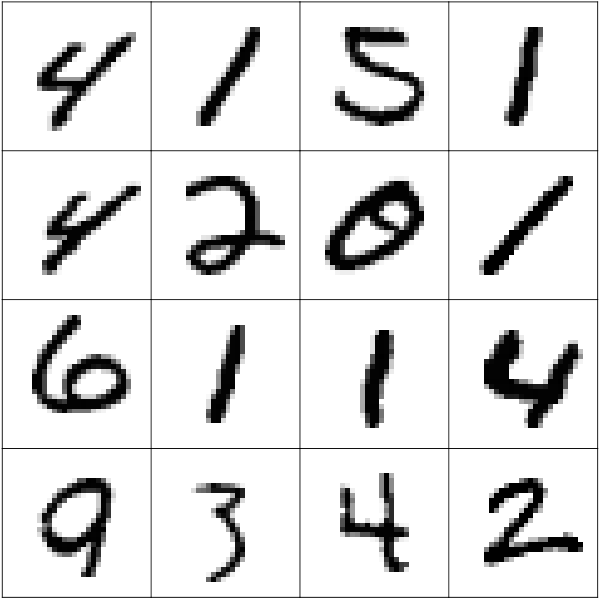
In order to better understand the structure of clusters in graphs, let us consider some examples constructed from real-world data. We begin by considering the well-known MNIST dataset which consists of 70,000 images of handwritten digits from 0 to 9. Each image has 28×2828\times 28 greyscale pixels, and each pixel takes a value from 0 to 255. This dataset is not given to us as a graph, but we can employ a common tool to convert almost any generic dataset into a graph: the kk nearest neighbour graph. To do this, we consider each image in the dataset to be a vertex in the graph, and connect each vertex vv to the vertices representing the images which are the ‘most similar’ to the image represented by vv. This construction is described more formally in Chapter 5. Figure 1.1 illustrates the kk nearest neighbour graph for a randomly chosen subset of the data.
Refer to caption
(a)
Refer to caption
(b)
Figure 1.1: (a) Example images from the MNIST dataset. (b) The kk nearest neighbour graph of a random subset of the MNIST dataset, for k=3k=3. The graph has a cluster corresponding to each digit.

Notice that in the constructed graph there are 10 clusters, which correspond to the ground truth clusters of images representing each digit. A vertex in a given cluster tends to be more strongly connected with other vertices inside the same cluster than with vertices in other clusters. There is also additional high-level structure due to the relative similarity of different digits. For example, the cluster representing the digit 4 has more connections with the cluster representing 9 than the one representing 6. This is the high-level structure which has been overlooked in previous clustering algorithms, and we study such structures in more detail in Chapter 5.

We will also look at another learning task for image data: image segmentation. In this case, we are given an arbitrary image, and the goal is to partition the pixels into some number of clusters such that each cluster corresponds to a different region of the image. This time, we will construct a graph from a single image in the following way: we first represent each pixel in the image by a point (r,g,b,x,y)⊺∈ℝ5(r,g,b,x,y)^{\intercal}\in\mathbb{R}^{5} where r,g,b∈[1,255]r,g,b\in[1,255] are the red, green, and blue values of the pixel and xx and yy are the coordinates of the pixel in the image. Then, we construct the similarity graph by taking each pixel to be a vertex in the graph, and for every pair of pixels 𝒖,𝒗∈ℝ5{\bm{u}},{\bm{v}}\in\mathbb{R}^{5}, we add an edge with weight exp(−‖𝒖−𝒗‖2/2σ2)\exp(-\left\|{\bm{u}}-{\bm{v}}\right\|^{2}/2\sigma^{2}) for some parameter σ\sigma. Notice that this graph combines the spatial and colour information of each pixel, such that we might expect each region of the image to be a separate cluster in the graph. We can then use a graph clustering algorithm to find these regions and segment the image. Once again, we can reasonably expect that the clusters in the graph constructed from the image will have some high-level structure. For example, a cluster representing a given region of the image will be more closely related to clusters of pixels with similar colours, or clusters representing neighbouring regions. We will see in Chapter 5 that this structure of clusters allows us to develop an improved graph-based image segmentation algorithm than the ones previously studied in the literature, and the results of this algorithm are also shown in Figure 1.2.

Refer to caption
(a) Original Image
Refer to caption
(b) Segmented Image
Figure 1.2: An example of image segmentation using the clustering algorithm in Chapter 5.

Finally, we will consider a completely different example dataset in which we are interested in learning the structure of clusters in a graph. The interstate dispute dataset records every military dispute between pairs of countries during 1816–2010, including the level of hostility resulting from the dispute and the number of casualties if applicable. This dataset already has a natural graph structure: for a given time period, we can construct a graph from the data by representing each country with a vertex and adding an edge between each pair of countries weighted according to the severity of their military disputes. Notice that since the edges in this graph represent a ‘negative’ relationship between countries, we would expect that a cluster of allied countries would not contain many edges inside the cluster. On the other hand, two different clusters might be densely connected to each other when there are two groups of opposing countries. If we wish to develop an algorithm for finding the clusters in this graph, clearly we must take the high-level structure into account and most existing graph clustering algorithms will not perform well. In Chapter 6, we will develop an algorithm capable of learning the clusters in this dataset which correspond to the underlying geopolitical relationships between countries. Figure 1.3 demonstrates that from this dataset, our algorithm is able to identify changes in geopolitics over time, including the changing roles of Russia, Japan, and Eastern Europe during the 20th century.

Refer to caption
(a) 1900-1950
Refer to caption
(b) 1990-2010
Figure 1.3: Clusters found by the algorithm from Chapter 6 on the interstate dispute dataset. For any given time period and using the USA as a ‘seed’, the algorithm returns two densely connected clusters representing groups of allied countries. The results are well explained by geopolitics, and capture the changing political picture during the 20th century.

Although our highlighted examples come from different domains and the method used to construct a graph is different in each case, their common theme is that the clusters in the generated graphs have a significant high-level structure. In this thesis we will see that these structures can be learned efficiently through our newly developed algorithms and that the cluster structure can be used to significantly improve the performance of spectral clustering. Throughout the thesis, we will touch on a wide variety of techniques from the field of algorithmic spectral graph theory, which studies the matrix representations of graphs and applies the algebraic properties of these matrices to design efficient algorithms. Along the way, we will examine the classical spectral clustering algorithm (Chapters 4 and 5), random walks and local algorithms (Chapter 6), and the recently emerging spectral hypergraph theory based on non-linear heat diffusion operators (Chapter 7). The newly developed techniques are all extensively evaluated on real-world datasets including those introduced above, and the results demonstrate a wide applicability for learning the structure of clusters in natural datasets. The remainder of the thesis is organised as follows.

  • •

    Chapter 2 introduces the basic mathematical concepts and notation which is used throughout the thesis, including a brief introduction to linear algebra, graphs, and hypergraphs. Additionally, this chapter introduces the field of spectral graph theory, on which most of the results in this thesis are based.

  • •

    Chapter 3 describes the previous work which is most related to the methods and results presented in later chapters. This includes a detailed description of the history of spectral graph partitioning, techniques for local graph clustering, and spectral hypergraph theory. This chapter forms an important reference in order to understand the technical material of the thesis.

  • •

    Chapter 4 studies spectral clustering, and presents a tighter analysis on its performance. This result explains why spectral clustering works under a much weaker and more natural condition than the ones previously studied in the literature, and helps to close the gap between the theoretical guarantees of the spectral clustering algorithm and its excellent empirical performance. This chapter is largely based on Sections 3 and 4 of Macgregor and Sun [MS22].

  • •

    Chapter 5 builds on the theoretical guarantees of the previous chapter and shows that, when the clusters of the underlying graph have certain structures, spectral clustering with fewer than kk eigenvectors is able to produce better output than classical spectral clustering in which kk eigenvectors are employed, where kk is the number of clusters. This chapter includes experiments on the MNIST dataset and the BSDS dataset for image segmentation, and demonstrates improved clustering performance over previous methods. This chapter is based on Sections 5 and 6 of Macgregor and Sun [MS22].

  • •

    Chapter 6 considers efficient learning of the structure of clusters with local algorithms, whose runtime depends only on the size of the target clusters and is independent of the underlying input graph. The experimental part of the chapter focuses on graphs like the interstate dispute dataset, in which clusters are densely connected to each other, and demonstrates that certain structures of clusters can be learned efficiently in the local setting. This chapter is based on Macgregor and Sun [MS21b].

  • •

    Finally, Chapter 7 studies the problem of learning densely connected clusters in hypergraphs. The developed algorithm is based on a new heat diffusion process, whose analysis extends a sequence of recent work on the spectral theory of hypergraphs. It allows the structure of clusters to be learned in datasets modelling higher-order relations of objects and can be applied to efficiently analyse many complex datasets occurring in practice. This chapter is based on Macgregor and Sun [MS21a].

Chapter 2Preliminaries

This chapter introduces the basic technical concepts which form the prerequisites for understanding the material in this thesis. Although most of the concepts listed here are standard, everything is included so that the thesis is as self-contained as possible. The chapter is divided into six sections. Section 2.1 defines some basic mathematical notation; Section 2.2 gives a brief introduction to concepts from linear algebra; Section 2.3 introduces graphs and spectral graph theory; Section 2.4 defines hypergraphs; Section 2.5 defines asymptotic notation used in the analysis of algorithms; finally, Section 2.6 defines the metrics used to evaluate clustering algorithms.

2.1 Basic Notation

Let us first define some of the mathematical notation used throughout the thesis. The set of real numbers is given by ℝ\mathbb{R}, the set of integers is ℤ\mathbb{Z}, and the set of complex numbers is ℂ\mathbb{C}. Occasionally, ℝ≥0\mathbb{R}_{\geq 0} or ℤ≥0\mathbb{Z}_{\geq 0} are used to restrict these sets to have non-negative values. For any n∈ℤ≥0n\in\mathbb{Z}_{\geq 0}, the notation [n][n] is used to mean {1,2,…,n}\{1,2,\ldots,n\}. For some logical proposition XX, the expression [X]\boldsymbol{\left[\vphantom{X}\right.}X\boldsymbol{\left.\vphantom{X}\right]} is equal to 11 if XX is true, or 00 otherwise. For example, we say that [a=b]\boldsymbol{\left[\vphantom{a=b}\right.}a=b\boldsymbol{\left.\vphantom{a=b}\right]} is equal to 11 if a=ba=b, and it is equal to 00 otherwise. For any operators f,g:ℝn→ℝnf,g:\mathbb{R}^{n}\rightarrow\mathbb{R}^{n}, we define f∘g:ℝn→ℝnf\circ g:\mathbb{R}^{n}\rightarrow\mathbb{R}^{n} by (f∘g)​(v)≜f⁡(g⁡(v))\left(f\circ g\right)(v)\triangleq f(g(v)) for any vv. Given two sets A{A} and B{B}, the set difference is expressed as A∖B{A}\setminus{B}. The symmetric difference between the sets AA and BB is given by A​△​B≜(A∖B)∪(B∖A){A}\triangle{B}\triangleq\left({A}\setminus{B}\right)\cup\left({B}\setminus{A}\right). When A{A} is a subset of some universe U{U}, the complement of A{A} is given by A¯≜U∖A\overline{{A}}\triangleq{U}\setminus{A}. For any set A{A}, we use 2A2^{A} to denote the power set of A{A}; that is, 2A2^{A} is the set consisting of all possible subsets of A{A}.

2.2 Linear Algebra

The subject of this thesis lies at the intersection of linear algebra and graph theory. As such, let us review some basic concepts in linear algebra. A vector 𝒙∈ℝn{\bm{x}}\in\mathbb{R}^{n} is written as (𝒙⁡(1),𝒙⁡(2),…,𝒙⁡(n))⊺({\bm{x}}(1),{\bm{x}}(2),\ldots,{\bm{x}}(n))^{\intercal}. Notice that we use 𝒙⁡(i){\bm{x}}(i) to refer to the ii-th element in the vector 𝒙{\bm{x}}. Subscripts, such as 𝒙i{\bm{x}}_{i}, are used to distinguish between different vectors. For a vector 𝒙∈ℝn{\bm{x}}\in\mathbb{R}^{n} and a set A⊆[n]{A}\subseteq[n], let 𝒙⁡(A)=∑i∈A𝒙⁡(i){\bm{x}}({A})=\sum_{i\in A}{\bm{x}}(i). For any vectors 𝒙,𝒚∈ℝn{\bm{x}},{\bm{y}}\in\mathbb{R}^{n}, we write 𝒙⪯𝒚{\bm{x}}\preceq{\bm{y}} if it holds for all vv that 𝒙⁡(v)≤𝒚⁡(v){\bm{x}}(v)\leq{\bm{y}}(v). We will use 𝟏n∈ℝn{\bm{1}}_{n}\in\mathbb{R}^{n} to represent the vector with 𝟏n​(i)=1{\bm{1}}_{n}(i)=1 for all i∈[n]i\in[n] and 𝟎n{\bm{0}}_{n} to represent the vector with 𝟎n​(i)=0{\bm{0}}_{n}(i)=0. For any vector 𝒙{\bm{x}}, we define the support of 𝒙{\bm{x}} to be supp⁡(𝒙)={u:𝒙⁡(u)≠0}\mathrm{supp}({\bm{x}})=\{u:{\bm{x}}(u)\neq 0\}. Given any two vectors 𝒗,𝒖∈ℝn{\bm{v}},{\bm{u}}\in\mathbb{R}^{n}, the inner product of 𝒗{\bm{v}} and 𝒖{\bm{u}} is written as ⟨𝒗,𝒖⟩\left\langle{\bm{v}},{\bm{u}}\right\rangle or 𝒗⊺​𝒖{\bm{v}}^{\intercal}{\bm{u}} and defined to be ∑i=1n𝒗⁡(i)​𝒖​(i)\sum_{i=1}^{n}{\bm{v}}(i){\bm{u}}(i). Throughout the thesis we will use the Euclidean norm, defined for any 𝒗∈ℝn{\bm{v}}\in\mathbb{R}^{n} as

‖𝒗‖=⟨𝒗,𝒗⟩=∑i=1n𝒗​(i)2.\left\|{\bm{v}}\right\|=\sqrt{\left\langle{\bm{v}},{\bm{v}}\right\rangle}=\sqrt{\sum_{i=1}^{n}{\bm{v}}(i)^{2}}.

Given a set of vectors {𝒗1,…,𝒗n}\{{\bm{v}}_{1},\ldots,{\bm{v}}_{n}\}, their span is denoted by span⁡(𝒗1,…​𝒗n)\mathrm{span}({\bm{v}}_{1},\ldots{\bm{v}}_{n}) and is defined to be the set of vectors 𝒙{\bm{x}} which can be written as a linear combination of 𝒗1,…,𝒗n{\bm{v}}_{1},\ldots,{\bm{v}}_{n}. That is, 𝒙∈span⁡(𝒗1,…,𝒗n){\bm{x}}\in\mathrm{span}({\bm{v}}_{1},\ldots,{\bm{v}}_{n}) if and only if

𝒙=∑i=1nci​𝒗i{\bm{x}}=\sum_{i=1}^{n}c_{i}{\bm{v}}_{i}

for some numbers c1,…,cn∈ℝc_{1},\ldots,c_{n}\in\mathbb{R}.

Given a matrix 𝐌∈ℝn×m{\mathbf{M}}\in\mathbb{R}^{n\times m}, the expression 𝐌⁡(i,j){\mathbf{M}}(i,j) is the element in the ii-th row and jj-th column of the matrix. An eigenvector of a matrix 𝐌∈ℝn×n{\mathbf{M}}\in\mathbb{R}^{n\times n} is any vector 𝒗∈ℝn{\bm{v}}\in\mathbb{R}^{n} such that 𝒗≠𝟎n{\bm{v}}\neq{\bm{0}}_{n} and

𝐌​𝒗=λ​𝒗{\mathbf{M}}{\bm{v}}=\lambda{\bm{v}}

for some λ∈ℝ\lambda\in\mathbb{R}, and λ\lambda is called an eigenvalue. When discussing some matrix 𝐌∈ℝn×n{\mathbf{M}}\in\mathbb{R}^{n\times n}, we often use λ1,…,λn\lambda_{1},\ldots,\lambda_{n} to denote the eigenvalues of 𝐌{\mathbf{M}} and 𝒇1,…​𝒇n{\bm{f}}_{1},\ldots{\bm{f}}_{n} for the eigenvectors. Occasionally, we consider matrices with complex-valued entries. Recall that for any complex number x=a+b⋅ix=a+b\cdot\mathit{i}, the complex conjugate of xx is given by x¯=a−b⋅i\overline{x}=a-b\cdot\mathit{i}. For any 𝐌∈ℂn×n{\mathbf{M}}\in\mathbb{C}^{n\times n}, the conjugate transpose of 𝐌{\mathbf{M}} is written as 𝐌†{\mathbf{M}}^{\dagger}, and is constructed by taking the transpose of 𝐌{\mathbf{M}} and replacing each entry with its complex conjugate. A matrix 𝐌{\mathbf{M}} is said to be Hermitian if 𝐌=𝐌†{\mathbf{M}}={\mathbf{M}}^{\dagger}. A real matrix 𝐌{\mathbf{M}} is positive semi-definite (PSD) if and only if it holds that

𝒙⊺​𝐌​𝒙≥0{\bm{x}}^{\intercal}{\mathbf{M}}{\bm{x}}\geq 0

for all 𝒙∈ℝn{\bm{x}}\in\mathbb{R}^{n}. It is equivalent to say that all of the eigenvalues of 𝐌{\mathbf{M}} are non-negative.

The following theorem, known as the Courant-Fischer Theorem, characterises the eigenvectors and eigenvalues of a symmetric matrix with respect to an optimisation over ℝn\mathbb{R}^{n}.

Theorem 2.1 (Courant-Fischer Theorem).

Let 𝐌{\mathbf{M}} be a real symmetric matrix with eigenvalues λ1≤…≤λn\lambda_{1}\leq\ldots\leq\lambda_{n}. Then

λk=minS⊂ℝndim⁡(S)=k⁡max𝒙∈S𝒙≠𝟎n​𝒙⊺​𝐌​𝒙𝒙⊺​𝒙,\lambda_{k}=\min_{\begin{subarray}{c}S\subset\mathbb{R}^{n}\\ \mathrm{dim}(S)=k\end{subarray}}\hskip 5.0pt\max_{\begin{subarray}{c}{\bm{x}}\in S\\ {\bm{x}}\neq{\bm{0}}_{n}\end{subarray}}\frac{{\bm{x}}^{\intercal}{\mathbf{M}}{\bm{x}}}{{\bm{x}}^{\intercal}{\bm{x}}},

where the minimisation is taken over all kk dimensional subspaces of ℝn\mathbb{R}^{n}.

2.3 Graphs

An undirected graph G=(V,E,w){G}=({V},{E},{w}) is defined by a set of vertices V{V}, a set of edges E{E}, and a weight function w:V×V→ℝ≥0{w}:{V}\times{V}\rightarrow\mathbb{R}_{\geq 0}. Every edge e∈Ee\in{E} is an unordered pair {v,u}\{v,u\} where v,u∈Vv,u\in{V} and v∼uv{\sim}u is used to mean that {v,u}∈E\{v,u\}\in{E}. The weight function w{w} is defined such that w⁡(v,u)>0{w}(v,u)>0 if {v,u}∈E\{v,u\}\in{E} and w⁡(v,u)=0{w}(v,u)=0 otherwise. Sometimes, the weight function ww is omitted when discussing a graph and in this case the weight of every edge can be taken to be 11. In this thesis, we consider only graphs with non-negative edge weights. A directed graph is defined similarly to an undirected graph, but in this case each edge e∈Ee\in{E} is an ordered pair (u,v)(u,v). Unless otherwise specified, the graphs defined in this thesis are undirected. Sometimes, the vertex and edge sets of different graphs are distinguished by subscript, such as G=(VG,EG,wG){G}=({V}_{G},{E}_{G},{w}_{G}) and H=(VH,EH,wH){H}=({V}_{H},{E}_{H},{w}_{H}).

Given some graph G=(V,E,w){G}=({V},{E},{w}), the number of vertices in a graph is commonly given by n=|V|n=\left\lvert{V}\right\rvert. The degree of any vertex v∈Vv\in{V} is defined by d⁡(v)≜∑u∈Vw⁡(v,u){d}(v)\triangleq\sum_{u\in{V}}{w}(v,u), and the set of neighbours of vv is N⁡(v)≜{u∈V:{v,u}∈E}{N}(v)\triangleq\{u\in{V}:\{v,u\}\in{E}\}. When G=(V,E){G}=({V},{E}) is a directed graph, for any v∈Vv\in{V} we use dout​(v){d}_{\mathrm{out}}(v) and din​(v){d}_{\mathrm{in}}(v) to express the number of edges with vv as the tail or the head, respectively. For any S⊂V{S}\subset{V}, we define volout​(S)=∑v∈Sdout​(v)\mathrm{vol}_{\mathrm{out}}({S})=\sum_{v\in{S}}{d}_{\mathrm{out}}(v), and volin​(S)=∑v∈Sdin​(v)\mathrm{vol}_{\mathrm{in}}({S})=\sum_{v\in{S}}{d}_{\mathrm{in}}(v).

For an undirected graph G=(V,E){G}=({V},{E}) and any S⊆V{S}\subseteq{V}, the volume of S{S} is defined by vol⁡(S)≜∑v∈Sd⁡(v)\mathrm{vol}({S})\triangleq\sum_{v\in{S}}{d}(v), and for two sets S1,S2⊆V{S}_{1},{S}_{2}\subseteq{V} let us define the weight between S1{S}_{1} and S2{S}_{2} by

w⁡(S1,S2)≜∑v∈S1∑u∈S2w⁡(v,u).{w}({S}_{1},{S}_{2})\triangleq\sum_{v\in{S}_{1}}\sum_{u\in{S}_{2}}{w}(v,u).

The conductance of S⊂V{S}\subset{V} is given by

Φ⁡(S)≜w⁡(S,S¯)min⁡{vol⁡(S),vol⁡(S¯)}.{\Phi}({S})\triangleq\frac{{w}({S},\overline{{S}})}{\min\{\mathrm{vol}({S}),\mathrm{vol}(\overline{{S}})\}}.

Notice that if Φ⁡(S)=0{\Phi}({S})=0, then S{S} is disconnected from the rest of the graph. Loosely, if Φ⁡(S){\Phi}({S}) is low, then there are only a small number of edges connecting S{S} to the rest of the graph and we can say that S{S} forms a cluster in the graph. The conductance of the graph G=(V,E){G}=({V},{E}) is given by

ΦG≜minS⊊VS≠∅⁡Φ⁡(S).{\Phi}_{G}\triangleq\min_{\begin{subarray}{c}{S}\subsetneq{V}\\ {S}\neq\emptyset\end{subarray}}{\Phi}({S}).

The boundary of S⊂V{S}\subset{V} is given by

∂(S)≜{{u,v}∈E:u∈S,v∉S}.\partial({S})\triangleq\{\{u,v\}\in{E}:u\in{S},v\not\in{S}\}.

The indicator vector of a set S⊆V{S}\subseteq{V} is given by 𝝌S∈ℝn{\bm{\chi}}_{S}\in\mathbb{R}^{n}, where

𝝌S​(v)={1if ​v∈S,0otherwise.{\bm{\chi}}_{S}(v)=\left\{\begin{array}[]{ll}1&\mbox{if }v\in{S},\\ 0&\mbox{otherwise.}\end{array}\right.

If S{S} contains only a single vertex vv, we can write 𝝌v{\bm{\chi}}_{v} instead of 𝝌{v}{\bm{\chi}}_{\{v\}}.

A graph G=(V,E){G}=({V},{E}) is said to be bipartite if the vertex set can be decomposed into disjoint sets L{L} and R{R} such that every edge e∈Ee\in{E} connects a vertex in L{L} with a vertex in R{R}. That is, for all e∈Ee\in{E}, it holds that e∩L≠∅e\cap{L}\neq\emptyset and e∩R≠∅e\cap{R}\neq\emptyset. A connected component of G{G} is any maximal set of vertices S⊆V{S}\subseteq{V} such that there is a path from any vertex in S{S} to every other vertex in S{S}.

2.3.1 Spectral Graph Theory

Having introduced linear algebra and graph theory, let us now take their intersection. Spectral graph theory is the study of the eigenvalues and eigenvectors of various matrices associated with a graph. This section gives a brief introduction to the key concepts in spectral graph theory, and Chapter 3 includes several specific results which are used in this thesis. For a comprehensive overview of the field, we refer the reader to Chung’s excellent book [Chu97].

Given a graph G=(V,E,w){G}=({V},{E},{w}) with nn vertices, let us label the vertices as V={v1,v2,…,vn}{V}=\{v_{1},v_{2},\ldots,v_{n}\}. Then, the adjacency matrix of G{G} is given by 𝐀∈ℝn×n{\mathbf{A}}\in\mathbb{R}^{n\times n} where 𝐀⁡(i,j)=w⁡(vi,vj){\mathbf{A}}(i,j)={w}(v_{i},v_{j}). The degree matrix 𝐃∈ℝn×n{\mathbf{D}}\in\mathbb{R}^{n\times n} is a diagonal matrix whose non-zero entries are 𝐃⁡(i,i)=d⁡(vi){\mathbf{D}}(i,i)={d}(v_{i}) for i∈[n]i\in[n]. A key object of study in spectral graph theory is the Laplacian matrix of G{G} which is defined to be

𝐋=𝐃−𝐀.{\mathbf{L}}={\mathbf{D}}-{\mathbf{A}}.

The most useful property of this operator is the expression given by its quadratic form. Given some vector 𝒙∈ℝn{\bm{x}}\in\mathbb{R}^{n}, the Laplacian quadratic form is given by

𝒙⊺​𝐋​𝒙=∑{u,v}∈Ew⁡(u,v)​(𝒙⁡(u)−𝒙⁡(v))2.{\bm{x}}^{\intercal}{\mathbf{L}}{\bm{x}}=\sum_{\{u,v\}\in{E}}{w}(u,v)\left({\bm{x}}(u)-{\bm{x}}(v)\right)^{2}.

It is also common to instead consider the normalised Laplacian matrix, which is defined as

𝐍=𝐃−12​𝐋𝐃−12=𝐈−𝐃−12​𝐀𝐃−12.{\mathbf{N}}={\mathbf{D}}^{-\frac{1}{2}}{\mathbf{L}}{\mathbf{D}}^{-\frac{1}{2}}={\mathbf{I}}-{\mathbf{D}}^{-\frac{1}{2}}{\mathbf{A}}{\mathbf{D}}^{-\frac{1}{2}}.

We also use the signless Laplacian operator defined as

𝐉≜𝐃+𝐀,{\mathbf{J}}\triangleq{\mathbf{D}}+{\mathbf{A}},

and its normalised counterpart

𝐙≜𝐃−12​𝐉𝐃−12.{\mathbf{Z}}\triangleq{\mathbf{D}}^{-\frac{1}{2}}{\mathbf{J}}{\mathbf{D}}^{-\frac{1}{2}}.

Many results in spectral graph theory focus on the eigenvectors and eigenvalues of the normalised Laplacian matrix. The nn eigenvalues are often given in order of increasing value, and are represented by λ1≤λ2≤…≤λn\lambda_{1}\leq\lambda_{2}\leq\ldots\leq\lambda_{n}. The corresponding eigenvectors are often denoted by 𝒇1,…,𝒇n{\bm{f}}_{1},\ldots,{\bm{f}}_{n}. Notice that the Laplacian matrix uniquely defines the original graph, and so the eigenvectors and eigenvalues of the Laplacian fully describe the graph. A recurring theme in spectral graph theory is that, in many cases, we can tell a lot about a graph from only a small number of eigenvalues and eigenvectors. The following basic results in spectral graph theory are not difficult to prove, and can be found in [Chu97].

  1. 1.

    The eigenvalues of 𝐍{\mathbf{N}} all lie between 00 and 22.

  2. 2.

    The smallest eigenvalue of 𝐍{\mathbf{N}} is always equal to 00.

  3. 3.

    If the graph has kk connected components, then the smallest eigenvalue of 𝐍{\mathbf{N}} has multiplicity kk.

  4. 4.

    The largest eigenvalue of 𝐍{\mathbf{N}} is equal to 22 if and only if the graph has a bipartite connected component.

Figure 2.1: A random graph sampled from SBM⁡(60,3,0.9,0.05)\mathrm{SBM}(60,3,0.9,0.05).

2.3.2 The Stochastic Block Model

It is useful to evaluate the performance of graph clustering algorithms on graphs with a known ground-truth clustering. A popular model for generating such random graphs is the stochastic block model (SBM), and we use several variants of this model throughout the thesis. For n,k∈ℤ≥0n,k\in\mathbb{Z}_{\geq 0} and p,q∈[0,1]p,q\in[0,1] the model SBM⁡(n,k,p,q)\mathrm{SBM}(n,k,p,q) defines a random graph on nn vertices in which the vertices are split evenly between kk clusters S1,…,Sk{S}_{1},\ldots,{S}_{k}. Every pair of vertices uu and vv are connected with probability

  • •

    pp if they are in the same cluster, and

  • •

    qq otherwise.

Figure 2.1 shows an example graph drawn from the stochastic block model. When p>qp>q, the stochastic block model typically generates graphs with a ground-truth cluster structure which makes it a useful model for evaluating the performance of graph clustering algorithms. For the interested reader, there is an extensive literature on several variants of the stochastic block model [Abb17, KMS16].

2.4 Hypergraphs

A hypergraph H=(V,E,w){H}=({V},{E},{w}) is defined by a vertex set V{V}, a set of edges E⊆2V{E}\subseteq 2^{V} and a weight function w:E→ℝ≥0w:{E}\rightarrow\mathbb{R}_{\geq 0}. The difference between a graph and a hypergraph is that each edge in a graph connects exactly two vertices while edges in a hypergraph can contain any number of vertices. Note that this means a graph is a special case of a hypergraph. Figure 2.2 shows an example hypergraph.

Figure 2.2: An example of a 33-uniform hypergraph with 66 vertices and 44 edges

Let H=(V,E,w){H}=({V},{E},{w}) be a hypergraph with n=|V|n=\left\lvert{V}\right\rvert vertices. For any vertex v∈Vv\in{V}, the degree of vv is defined by d(v)≜∑e∈Ew(e)⋅[v∈e]{d}(v)\triangleq\sum_{e\in{E}}{w}(e)\cdot\boldsymbol{\left[\vphantom{v\in e}\right.}v\in e\boldsymbol{\left.\vphantom{v\in e}\right]}, recalling that [X]=1\boldsymbol{\left[\vphantom{X}\right.}X\boldsymbol{\left.\vphantom{X}\right]}=1 if event XX holds and [X]=0\boldsymbol{\left[\vphantom{X}\right.}X\boldsymbol{\left.\vphantom{X}\right]}=0 otherwise. The rank of edge e∈Ee\in{E} is defined to be the total number of vertices in ee and is written as rank⁡(e)\mathrm{rank}(e). A hypergraph is said to be 𝒓\bm{r}-uniform if every edge e∈Ee\in{E} has rank rr.

2.5 Asymptotic Notation

When studying the running time of algorithms, we are often interested in how the running time grows as a function of the size of the algorithm’s input. A useful tool to this end is asymptotic notation. Suppose we are given two functions f,g:ℝ→ℝf,g:\mathbb{R}\rightarrow\mathbb{R}. Then, we say that

f⁡(x)=O⁡(g⁡(x))f(x)=O\!\left(g(x)\right)

if there exist constants c,t∈ℝc,t\in\mathbb{R} such that for all x≥tx\geq t, it holds that f⁡(x)≤c⋅g⁡(x)f(x)\leq c\cdot g(x). For example, if f⁡(n)f(n) gives the running time of some algorithm for an input of size nn, then f⁡(n)=O⁡(n)f(n)=O\!\left(n\right) tells us that for sufficiently large inputs, the running time of the algorithm is at most linear in nn. On the other hand,

f⁡(x)=Ω⁡(g⁡(x))f(x)=\Omega\!\left(g(x)\right)

tells us that there exist constants c,t∈ℝc,t\in\mathbb{R} such that for all x≥tx\geq t, it holds that f⁡(x)≥c⋅g⁡(x)f(x)\geq c\cdot g(x). In other words, f⁡(x)=Ω⁡(g⁡(x))f(x)=\Omega\!\left(g(x)\right) if and only if g⁡(x)=O⁡(f⁡(x))g(x)=O\!\left(f(x)\right). Finally, we can say that

f⁡(x)=Θ⁡(g⁡(x))f(x)=\Theta\!\left(g(x)\right)

if f⁡(x)=O⁡(g⁡(x))f(x)=O\!\left(g(x)\right) and f⁡(x)=Ω⁡(g⁡(x))f(x)=\Omega\!\left(g(x)\right). When discussing the running time of algorithms, it is common to use poly⁡(n)\mathrm{poly}(n) to represent some polynomial in nn and polylog⁡(n)\mathrm{polylog}(n) for some polynomial in log⁡(n)\log(n). Intuitively, O⁡(⋅)O\!\left(\cdot\right) gives an upper-bound on some function, and hides a constant factor. We can take this one step further and use O~​(⋅)\widetilde{O}\!\left(\cdot\right) to hide constants and logarithmic factors. For example, suppose f⁡(x)=100⋅x​log⁡(x)f(x)=100\cdot x\log(x). Then, we could say that f⁡(x)=O⁡(x​log⁡(x))f(x)=O\!\left(x\log(x)\right) or f​(x)=O~​(x)f(x)=\widetilde{O}\!\left(x\right).

Occasionally, we will use asymptotic notation in order to hide a fixed constant when we are not discussing the asymptotic behaviour of a function. For example, x=Ω⁡(y)x=\Omega(y) means that there exists a universal constant cc such that x≥c​yx\geq cy. This use of asymptotic notation is common throughout theoretical computer science [LOGT14, PSZ17].

2.6 Clustering Metrics

When evaluating the performance of a clustering algorithm, we would like to measure the similarity between the ground truth clusters and the clusters returned by the algorithm. The Rand Index [Ran71], also referred to as the clustering accuracy, is a common metric used for this purpose.

Suppose we are given a dataset with nn data points and kk clusters. The ground truth clusters are given by C1,…,Ck{C}_{1},\ldots,{C}_{k} and the clusters returned by our algorithm are S1,…,Sk{S}_{1},\ldots,{S}_{k}. Let σC:[n]→[k]\sigma_{\mathrm{C}}:[n]\xrightarrow{}[k] be a function which maps each data point to its ground truth cluster. That is, if j∈Cij\in{C}_{i} then σC​(j)=i\sigma_{\mathrm{C}}(j)=i. Let σS:[n]→[k]\sigma_{\mathrm{S}}:[n]\xrightarrow{}[k] be the equivalent function for the clusters S1,…,Sk{S}_{1},\ldots,{S}_{k}. Then, let

TP≜|{(i,j)∈[n]×[n]:i≠j∧σC​(i)=σC​(j)∧σS​(i)=σS​(j)}|\mathrm{TP}\triangleq\left\lvert\{(i,j)\in[n]\times[n]:i\neq j\land\sigma_{\mathrm{C}}(i)=\sigma_{\mathrm{C}}(j)\land\sigma_{\mathrm{S}}(i)=\sigma_{\mathrm{S}}(j)\}\right\rvert

be the number of pairs of data points which are in the same ground truth cluster and the same cluster returned by the algorithm. Similarly, let

TN≜|{(i,j)∈[n]×[n]:i≠j∧σC​(i)≠σC​(j)∧σS​(i)≠σS​(j)}|\mathrm{TN}\triangleq\left\lvert\{(i,j)\in[n]\times[n]:i\neq j\land\sigma_{\mathrm{C}}(i)\neq\sigma_{\mathrm{C}}(j)\land\sigma_{\mathrm{S}}(i)\neq\sigma_{\mathrm{S}}(j)\}\right\rvert

be the number of pairs of data points which the algorithm correctly identifies as belonging to different clusters. Then, the Rand Index is

RI≜TP+TN(n2).\mathrm{RI}\triangleq\frac{\mathrm{TP}+\mathrm{TN}}{\binom{n}{2}}.

That is, the Rand Index measures the proportion of pairs of data points which the algorithm correctly classifies as belonging to the same cluster or different clusters. While this is a natural definition, notice that even a baseline algorithm which assigns data points to clusters at random will achieve a non-zero Rand Index. To correct for this, the Adjusted Rand Index [GA17] normalises the Rand Index by the expected value for a random assignment. Further defining

FP≜|{(i,j)∈[n]×[n]:i≠j∧σC​(i)≠σC​(j)∧σS​(i)=σS​(j)}|\mathrm{FP}\triangleq\left\lvert\{(i,j)\in[n]\times[n]:i\neq j\land\sigma_{\mathrm{C}}(i)\neq\sigma_{\mathrm{C}}(j)\land\sigma_{\mathrm{S}}(i)=\sigma_{\mathrm{S}}(j)\}\right\rvert

and

FN≜|{(i,j)∈[n]×[n]:i≠j∧σC​(i)=σC​(j)∧σS​(i)≠σS​(j)}|,\mathrm{FN}\triangleq\left\lvert\{(i,j)\in[n]\times[n]:i\neq j\land\sigma_{\mathrm{C}}(i)=\sigma_{\mathrm{C}}(j)\land\sigma_{\mathrm{S}}(i)\neq\sigma_{\mathrm{S}}(j)\}\right\rvert,

the Adjusted Rand Index is given by

ARI≜2​(TP⋅TN−FP⋅FN)(TP+FN)​(TN+FN)+(TN+FP)​(TP+FP).\mathrm{ARI}\triangleq\frac{2\left(\mathrm{TP}\cdot\mathrm{TN}-\mathrm{FP}\cdot\mathrm{FN}\right)}{(\mathrm{TP}+\mathrm{FN})(\mathrm{TN}+\mathrm{FN})+(\mathrm{TN}+\mathrm{FP})(\mathrm{TP}+\mathrm{FP})}.

In contrast with the Rand Index, which gives a value between 00 and 11, the Adjusted Rand Index can give negative values. A random assignment of data points to clusters will give an expected Adjusted Rand Index of 00.

Chapter 3Related Work

The goal of this chapter is to provide a broad overview of the techniques related to the algorithms developed later in the thesis, and to serve as an introduction to spectral graph partitioning, local graph clustering, and spectral hypergraph theory. As well as placing the novel work of this thesis in the context of the related work in the field, this chapter also introduces several technical concepts which are built on in the later chapters. The structure of the chapter is given below.

  • •

    Section 3.1 gives an introduction to spectral graph partitioning, and describes several key points in the development of the field which underpins this thesis.

  • •

    Section 3.2 describes some recently developed techniques for finding clusters in graphs with specific structures of clusters.

  • •

    Section 3.3 introduces local graph clustering and describes two key algorithms based on the personalised Pagerank and evolving set process, respectively.

  • •

    Section 3.4 gives a brief overview of spectral hypergraph theory, with a focus on the hypergraph Laplacian operator recently developed by Chan et al. [CLTZ18].

3.1 Spectral Graph Partitioning

Spectral graph partitioning is the use of the eigenvectors of graph matrices to help with finding partitions (or clusters) in graphs. The roots of this idea stretch back to the 1970s, when Donath and Hoffman [DH72] first proposed to use the eigenvectors of the adjacency matrix for partitioning, although they gave no theoretical justification for this choice.

3.1.1 Fiedler Vector

In 1973, Fiedler [Fie73] proved a number of results relating the second smallest eigenvalue of the graph Laplacian to the combinatorial connectivity of the graph. This gave the first theoretical justification for using eigenvectors in graph partitioning. Many authors refer to the eigenvector corresponding to the second smallest eigenvalue of the Laplacian as the Fiedler vector of the graph. The corresponding eigenvalue is sometimes referred to as the algebraic connectivity of the graph.

3.1.2 Cheeger Inequality

In parallel to this, Cheeger [Che70] studied the connectivity of Riemannian manifolds, and proved an inequality relating the second smallest eigenvalue of the Laplacian operator to the connectivity of the manifold. The significance of Cheeger’s result for graph partitioning was demonstrated several years later, when Dodziuk [Dod84] and Alon [Alo86] independently proved (slightly weaker) versions of Cheeger’s inequality in the graph setting. Chung [Chu96] later tightened the result and proved the following theorem, which is commonly referred to as the Cheeger inequality in the context of spectral graph theory.

Theorem 3.1 (Cheeger Inequality).

Let G{G} be a graph and 𝐍G{\mathbf{N}}_{G} be its normalised Laplacian matrix with eigenvalues 0=λ1≤λ2≤…≤λn0=\lambda_{1}\leq\lambda_{2}\leq\ldots\leq\lambda_{n}. Then,

λ22≤ΦG≤2​λ2,\frac{\lambda_{2}}{2}\leq{\Phi}_{G}\leq\sqrt{2\lambda_{2}},

where ΦG{\Phi}_{G} is the conductance of GG.

The theorem relates the second smallest eigenvalue of the graph Laplacian to the conductance of the graph. While the theorem itself already provides significant evidence that the Laplacian spectrum may be helpful when partitioning graphs, its proof gives even more. The proof of the upper bound of Theorem 3.1 is constructive: it presents an algorithm which, given a graph G=(V,E){G}=({V},{E}), finds a set S⊂V{S}\subset{V} such that Φ⁡(S)≤2​λ2{\Phi}({S})\leq\sqrt{2\lambda_{2}}. The algorithm is formally described in Algorithm 1, and for any given graph the partition returned by this algorithm is often called the Cheeger cut of the given graph.

Compute the second smallest eigenvalue λ2\lambda_{2} of 𝐍G{\mathbf{N}}_{G}, and its eigenvector 𝒇2{\bm{f}}_{2}
Sort the vertices v1,…,vn∈VGv_{1},\ldots,v_{n}\in{V}_{G} such that 𝒇2​(v1)/d⁡(v1)≤…≤𝒇2​(vn)/d⁡(vn){\bm{f}}_{2}(v_{1})/\sqrt{{d}(v_{1})}\leq\ldots\leq{\bm{f}}_{2}(v_{n})/\sqrt{{d}(v_{n})}
Let i=arg​mini∈[n−1]⁡ΦG​({v1,…,vi})i=\argmin_{i\in[n-1]}{\Phi}_{G}(\{v_{1},\ldots,v_{i}\})
Return {v1,…,vi}\{v_{1},\ldots,v_{i}\}
Algorithm 1 SweepSet(G)({G})

It is worth noting that both sides of the Cheeger inequality are tight up to a constant, as demonstrated in Examples 3.1 and 3.2.

Example 3.1 (Tightness of Cheeger Inequality lower bound).

Let G{G} be the dd-dimensional hypercube graph. Then,

λ2=2d\lambda_{2}=\frac{2}{d}

and

Φ⁡(G)=2d−1d⋅2d−1=1d=λ22,{\Phi}({G})=\frac{2^{d-1}}{d\cdot 2^{d-1}}=\frac{1}{d}=\frac{\lambda_{2}}{2},

which demonstrates that the lower bound is tight.

Figure 3.1: A hypercube graph and the cut with minimum conductance.
Example 3.2 (Tightness of Cheeger Inequality upper bound).

Let G{G} be the cycle graph on nn vertices. Then,

λ2=2−2​cos⁡(2​πn)=O⁡(1n2),\lambda_{2}=2-2\cos\left(\frac{2\pi}{n}\right)=O\!\left(\frac{1}{n^{2}}\right),

using the fact that 1−cos⁡(x)=2​sin2⁡(x/2)1-\cos(x)=2\sin^{2}(x/2) and sin⁡(x)≤x\sin(x)\leq x. Moreover, we have that

ΦG=2n=Ω⁡(λ2),{\Phi}_{G}=\frac{2}{n}=\Omega\!\left(\sqrt{\lambda_{2}}\right),

which shows that the Cheeger inequality is tight up to a constant.

Figure 3.2: A cycle graph and the cut with minimum conductance.

Finally, Kwok et al. [KLL+13] gave the following improved version of the Cheeger inequality, which shows that λ2\lambda_{2} better approximates the conductance ΦG{\Phi}_{G} when there is a large gap between λ2\lambda_{2} and λ3\lambda_{3}.

Theorem 3.2 (Improved Cheeger Inequality).

Let G{G} be a graph, and 𝐍G{\mathbf{N}}_{G} be its normalised Laplacian matrix with eigenvalues 0=λ1≤λ2≤…≤λn0=\lambda_{1}\leq\lambda_{2}\leq\ldots\leq\lambda_{n}. Then, it holds for any 2≤k≤n2\leq k\leq n that

ΦG≤O⁡(k)​λ2λk,{\Phi}_{G}\leq O\!\left(k\right)\frac{\lambda_{2}}{\sqrt{\lambda_{k}}},

where ΦG{\Phi}_{G} is the conductance of GG.

3.1.3 Higher-order Cheeger Inequality

The Cheeger inequality clearly justifies the use of the second eigenvector of the graph Laplacian for partitioning a graph into two parts. This raises a natural question of whether the other eigenvalues give any information for partitioning the graph into more than two parts. Lee et al. [LOGT14] considered the 𝒌\bm{k}-way expansion constant of a graph, which generalises the conductance of a graph to a partitioning with more than two clusters.

Definition 3.1 (kk-way expansion).

Given a graph G{G}, the kk-way expansion is defined as

ρG​(k)≜minpartition​S1,…,Sk⁡maxi∈[k]​ΦG​(Si),{{\rho}_{G}}(k)\triangleq\min_{\mathrm{partition}~{S}_{1},\ldots,{S}_{k}}\max_{i\in[k]}{\Phi}_{G}({S}_{i}),

where the minimum is taken over all sets S1,…,Sk⊂VG{S}_{1},\ldots,{S}_{k}\subset{V}_{G} where Si∩Sj=∅{S}_{i}\cap{S}_{j}=\emptyset for all i≠ji\neq j and ⋃i=1kSi=VG\bigcup_{i=1}^{k}{S}_{i}={V}_{G}.

It is clear that ρG​(2)=ΦG{{\rho}_{G}}(2)={\Phi}_{G}, and so this generalises the definition of graph conductance. Lee et al. [LOGT14] proved the following theorem, which relates the kk-way expansion of a graph to the kk-th smallest eigenvalue of the normalised Laplacian.

Theorem 3.3 (Higher-order Cheeger Inequality).

Let G=(V,E){G}=({V},{E}) be a graph, and 𝐍G{\mathbf{N}}_{G} be its normalised Laplacian matrix with eigenvalues 0=λ1≤λ2≤…≤λn0=\lambda_{1}\leq\lambda_{2}\leq\ldots\leq\lambda_{n}. Then,

λk2≤ρG​(k)≤O⁡(k3)​λk,\frac{\lambda_{k}}{2}\leq{{\rho}_{G}}(k)\leq O\!\left(k^{3}\right)\sqrt{\lambda_{k}},

where ρG​(k){{\rho}_{G}}(k) is the kk-way expansion constant of G{G}.

Once again, the proof of this theorem is constructive, and gives an algorithm for finding clusters S1,…,Sk{S}_{1},\ldots,{S}_{k} satisfying the inequalities. The dependence on kk in the upper bound of Theorem 3.3 is needed, but it is not known if the inequality is tight [LOGT14].

3.1.4 Spectral Clustering

The spectral clustering algorithm was proposed over a decade before the higher-order Cheeger inequality [NJW01], and is widely used in practice due to its simplicity and empirical effectiveness. There are several variants of this algorithm since it is possible to use the adjacency matrix, Laplacian matrix, or normalised Laplacian matrix for constructing the spectral embedding [vL07]. However, they are all composed of the same three steps:

  1. 1.

    Compute kk eigenvectors of some graph matrix;

  2. 2.

    Embed the vertices of the graph into ℝk\mathbb{R}^{k} according to the values of the eigenvectors;

  3. 3.

    Apply a simple clustering algorithm, such as kk-means, to obtain the final clusters.

See Algorithm 2 for the formal description of spectral clustering.

Construct the normalised graph Laplacian matrix 𝐍G{\mathbf{N}}_{G}
Compute eigenvectors 𝒇1,…,𝒇k{\bm{f}}_{1},\ldots,{\bm{f}}_{k} of 𝐍G{\mathbf{N}}_{G} corresponding to the kk smallest eigenvalues
Embed each v∈VGv\in{V}_{G} to the point (𝒇1​(v),…,𝒇k​(v))⊺({\bm{f}}_{1}(v),\ldots,{\bm{f}}_{k}(v))^{\intercal}
Apply kk-means to the embedded vertices; partition VG{V}_{G} based on the output
Algorithm 2 SpectralCluster(G,k)({G},k)

Although spectral clustering has been used in practice for several decades, the theoretical justification for its good performance has seen some recent progress [PSZ17] and deserves further study. There are two technical approaches which are common when analysing spectral clustering. The first is to see that the algorithm solves a relaxation of a natural optimisation problem. For more details on this perspective, the reader can refer to the excellent tutorial of Von Luxburg [vL07]. The second comes from considering the structure of clusters in the eigenspace of the graph matrices. Ng et al. [NJW01] introduced this idea with the following observations, which are illustrated in Figure 3.3.

  1. 1.

    If the clusters in the input graph GG are disconnected, then the normalised Laplacian matrix 𝐍G{\mathbf{N}}_{G} is block diagonal. Therefore, the first kk eigenvectors of 𝐍G{\mathbf{N}}_{G} are the indicator vectors of the connected components.

  2. 2.

    If the clusters are then connected by a small number of edges, then the Laplacian matrix doesn’t change much, and accordingly the eigenvalues and eigenvectors of the Laplacian do not change too much.

  3. 3.

    As such, if a graph possesses a clear cluster structure, then the clusters are well separated in the spectral embedding.

→\xrightarrow{}[𝐁1𝟎𝟎𝟎𝐁2𝟎𝟎𝟎𝐁3]\begin{bmatrix}{\mathbf{B}}_{1}&{\mathbf{0}}&{\mathbf{0}}\\ {\mathbf{0}}&{\mathbf{B}}_{2}&{\mathbf{0}}\\ {\mathbf{0}}&{\mathbf{0}}&{\mathbf{B}}_{3}\end{bmatrix}→\xrightarrow{}Graph G{G}Normalised Laplacian 𝐍{\mathbf{N}}Spectral Embedding→\xrightarrow{}[𝐁1𝐂12𝐂13𝐂12⊺𝐁2𝐂23𝐂13⊺𝐂23⊺𝐁3]\begin{bmatrix}{\mathbf{B}}_{1}&{\mathbf{C}}_{12}&{\mathbf{C}}_{13}\\ {\mathbf{C}}_{12}^{\intercal}&{\mathbf{B}}_{2}&{\mathbf{C}}_{23}\\ {\mathbf{C}}_{13}^{\intercal}&{\mathbf{C}}_{23}^{\intercal}&{\mathbf{B}}_{3}\end{bmatrix}→\xrightarrow{}Graph G{G}Normalised Laplacian 𝐍{\mathbf{N}}Spectral Embedding
Figure 3.3: An illustration of the intuition behind spectral clustering. If the clusters are disconnected, then the Laplacian is block diagonal and the spectral embedding perfectly separates the clusters. If a small number of edges are added between the clusters, then the embedding doesn’t change ‘too much’.

Peng et al. [PSZ17] built on this intuition and proved that, not only are the clusters well separated in the spectral embedding, but the output of the kk-means algorithm is guaranteed to correctly cluster most of the vertices. To quantify the ‘clusterability’ of a given graph GG, they introduced the parameter Υ⁡(k)\Upsilon(k) defined as follows:

Definition 3.2.

For a graph G{G}, let λ1≤λ2≤…≤λn\lambda_{1}\leq\lambda_{2}\leq\ldots\leq\lambda_{n} be the eigenvalues of the normalised Laplacian matrix 𝐍G{\mathbf{N}}_{G}. Then,

Υ⁡(k)≜λk+1ρ⁡(k),\Upsilon(k)\triangleq\frac{\lambda_{k+1}}{{\rho}(k)},

where ρ⁡(k){\rho}(k) is the kk-way expansion constant.

To understand the motivation behind this definition, suppose that a graph G=(V,E){G}=({V},{E}) contains exactly kk clusters with low conductance. That is,

  1. 1.

    there is a partition of V{V} into kk sets S1,…,Sk{S}_{1},\ldots,{S}_{k} such that maxi∈[k]⁡Φ⁡(Si)\max_{i\in[k]}{\Phi}({S}_{i}) is low, and

  2. 2.

    for any partition of V{V} into k+1k+1 sets S1,…,Sk+1{S}_{1},\ldots,{S}_{k+1}, there is some i∈[k+1]i\in[k+1] such that Φ⁡(Si){\Phi}({S}_{i}) is high.

Then, by the definition of ρ⁡(k){\rho}(k), the denominator of Υ⁡(k)\Upsilon(k) is low, and by the higher-order Cheeger inequality (Theorem 3.3), the numerator is high. Thus, a large value of Υ⁡(k)\Upsilon(k) indicates that there are exactly kk low-conductance clusters in the graph. The definition of Υ⁡(k)\Upsilon(k) also closely resembles the widely-used eigen-gap heuristic for spectral clustering [NJW01, vL07], which suggests that spectral clustering works when the value of |λk+1−λk|\left\lvert\lambda_{k+1}-\lambda_{k}\right\rvert is much larger than |λk−λk−1|\left\lvert\lambda_{k}-\lambda_{k-1}\right\rvert.

Peng et al. [PSZ17] prove that for graphs with a high value of Υ⁡(k)\Upsilon(k), the eigenvectors of the Laplacian are close to the indicator vectors of the optimal clusters. Let S1,…,Sk⊂V{S}_{1},\ldots,{S}_{k}\subset{V} be the optimal clusters which achieve the kk-way expansion ρ⁡(k){\rho}(k), then the normalised indicator vector of each cluster Si{S}_{i} is defined as

𝒈¯i=𝐃12​𝝌Si‖𝐃12​𝝌Si‖.\bar{{\bm{g}}}_{i}=\frac{{\mathbf{D}}^{\frac{1}{2}}{\bm{\chi}}_{{S}_{i}}}{\left\|{\mathbf{D}}^{\frac{1}{2}}{\bm{\chi}}_{{S}_{i}}\right\|}.

Their result is given in the following theorem.

Theorem 3.4 ([PSZ17], Theorem 1.1).

Let G{G} be a graph with Υ⁡(k)=Ω⁡(k2)\Upsilon(k)=\Omega\!\left(k^{2}\right), and let 𝐟1,…,𝐟n{\bm{f}}_{1},\ldots,{\bm{f}}_{n} be the eigenvectors of 𝐍G{\mathbf{N}}_{G} corresponding to eigenvalues λ1≤…≤λn\lambda_{1}\leq\ldots\leq\lambda_{n}. Then,

  1. 1.

    for every 𝒈¯i\bar{{\bm{g}}}_{i}, there is a linear combination of {𝒇i}i=1k\{{\bm{f}}_{i}\}_{i=1}^{k} called 𝒇^i\widehat{{\bm{f}}}_{i} such that ‖𝒈¯i−𝒇^i‖≤1/Υ⁡(k)\left\|\bar{{\bm{g}}}_{i}-\widehat{{\bm{f}}}_{i}\right\|\leq 1/\Upsilon(k);

  2. 2.

    for every 𝒇i{\bm{f}}_{i}, there is a linear combination of {𝒈¯i}i=1k\{\bar{{\bm{g}}}_{i}\}_{i=1}^{k}, called 𝒈^i\widehat{{\bm{g}}}_{i}, such that ‖𝒇i−𝒈^i‖2≤1.1​k/Υ⁡(k)\left\|{\bm{f}}_{i}-\widehat{{\bm{g}}}_{i}\right\|^{2}\leq 1.1k/\Upsilon(k).

Peng et al. [PSZ17] used this to prove an upper bound on the number of vertices misclassified by the kk-means clustering step of the spectral clustering algorithm.

Theorem 3.5 ([PSZ17], Theorem 1.2).

Let G{G} be a graph with Υ⁡(k)=Ω⁡(k3)\Upsilon(k)=\Omega\!\left(k^{3}\right). Let A1,…,Ak{A}_{1},\ldots,{A}_{k} be the clusters found by spectral clustering, and let the optimal correspondent of Ai{A}_{i} be Si{S}_{i}. Then, it holds for any i∈[k]i\in[k] that

vol⁡(Ai​△​Si)vol⁡(Si)=O⁡(k3/Υ⁡(k)).\frac{\mathrm{vol}({A}_{i}\triangle{S}_{i})}{\mathrm{vol}({S}_{i})}=O\!\left(k^{3}/\Upsilon(k)\right).

Kolev and Melhorn [KM16] and Mizutani [Miz21] developed similar results under the weaker assumptions of Υ⁡(k)=Ω⁡(k2)\Upsilon(k)=\Omega(k^{2}) and Υ⁡(k)=Ω⁡(k)\Upsilon(k)=\Omega(k) respectively, although their results are not directly comparable since they use a slightly different definition of the gap Υ⁡(k)\Upsilon(k).

3.2 Clustering Structured Graphs

Spectral clustering gives an excellent starting point for the subject of graph partitioning; however, the classical analysis is usually based only on the assumption that the clusters are sparsely connected to each other and does not take into account the high-level structure of clusters. As demonstrated in Chapter 1, graphs created from real-world data often exhibit a high-level structure, and this section describes techniques for learning clusters in such graphs.

3.2.1 Partitioning Almost-Bipartite Graphs

Let us start by considering the case of graphs exhibiting heterophily. That is, graphs in which vertices have a tendency to share connections with those in a different cluster to their own.11 1 For completeness, the opposite of heterophily is homophily, in which vertices are more likely to share edges with other vertices in the same cluster. An example of such a graph is the inter-state dispute graph introduced in Chapter 1. More generally, graphs in which edges represent ‘negative’ relationships tend to exhibit heterophily.

A bipartite graph is a ‘perfect’ example of a two-cluster graph with heterophily. Of course, it is not difficult to separate a bipartite graph into its two clusters, but what if the graph is only almost bipartite? To answer this, Bauer and Jost [BJ13] and Trevisan [Tre12] introduced the bipartiteness of two sets L,R⊂VG{L},{R}\subset{V}_{G}, which measures how close the sets L{L} and R{R} are to forming a bipartite connected component.

Definition 3.3 (Bipartiteness).

Given a graph G=(V,E){G}=({V},{E}) and two clusters L,R⊂V{L},{R}\subset{V}, the bipartiteness of L{L} and R{R} is

β⁡(L,R)≜1−2​w​(L,R)vol⁡(L∪R).{\beta}({L},{R})\triangleq 1-\frac{2{w}({L},{R})}{\mathrm{vol}({L}\cup{R})}.

The bipartiteness of the graph G{G} is given by

βG≜minL,R⊂VGL∩R=∅⁡β⁡(L,R).{\beta}_{G}\triangleq\min_{\begin{subarray}{c}{L},{R}\subset{V}_{G}\\ {L}\cap{R}=\emptyset\end{subarray}}{\beta}({L},{R}).

Notice that β⁡(L,R)=0{\beta}({L},{R})=0 if L{L} and R{R} form a bipartite and connected component of G{G}. Given a graph G{G}, let 0=λ1≤λ2≤…≤λn≤20=\lambda_{1}\leq\lambda_{2}\leq\ldots\leq\lambda_{n}\leq 2 be the eigenvalues of the normalised Laplacian 𝐍G{\mathbf{N}}_{G}. It is a classical result in spectral graph theory that λn=2\lambda_{n}=2 if and only if βG=0{\beta}_{G}=0, and so a natural question is whether there is an analogue of the Cheeger inequality which connects the bipartiteness of a graph with the largest eigenvalue λn\lambda_{n}. Bauer and Jost [BJ13] and Trevisan [Tre12] independently showed that this is indeed the case with the following theorem.

Theorem 3.6.

Given a graph G{G}, let λ1≤λ2≤…≤λn\lambda_{1}\leq\lambda_{2}\leq\ldots\leq\lambda_{n} be the eigenvalues of the normalised Laplacian 𝐍G{\mathbf{N}}_{G}. Then,

2−λn2≤βG≤2​(2−λn),\frac{2-\lambda_{n}}{2}\leq{\beta}_{G}\leq\sqrt{2(2-\lambda_{n})},

where βG{\beta}_{G} is the bipartiteness of the graph.

Trevisan used this result to develop a novel approximation algorithm for the MAX-CUT problem. Soto [Sot15] improved Trevisan’s analysis and showed that the algorithm achieves an approximation ratio of 0.6142470.614247. Liu [Liu15] generalised Theorem 3.6 and proved a higher-order version of this inequality which links the top eigenvalues of a graph Laplacian to the bipartiteness of multiple clusters in the graph.

The problem of learning the clusters in graphs exhibiting heterophily has also been studied from a supervised and semi-supervised learning perspective, such as in [MYZ+11, PWC+19, ZYZ+20]. These techniques are not covered in detail here since the focus of this thesis is on algorithms for unsupervised learning.

3.2.2 Learning Clusters from Edge Directions

In the preceding sections, we considered algorithms for learning clusters which are defined by sparse (or dense) connections. In this section, we consider directed graphs in which the clusters are defined by the directions of their connecting edges.

Cucuringu et al. [CLSZ20] studied this problem and introduced the so-called cut imbalance between two clusters S1,S2⊂V{S}_{1},{S}_{2}\subset{V}, which measures the imbalance of edge directions between the clusters. They proposed to use the Hermitian adjacency matrix of a directed graph to find clusters with a large cut imbalance. The Hermitian adjacency matrix of a directed graph G{G} is the matrix 𝐀h∈ℂn×n{\mathbf{A}}_{h}\in\mathbb{C}^{n\times n} where 𝐀h​(u,v)=𝐀h​(v,u)¯=i{\mathbf{A}}_{h}(u,v)=\overline{{\mathbf{A}}_{h}(v,u)}=\mathit{i} if G{G} contains an edge from uu to vv and 𝐀h​(u,v)=𝐀h​(v,u)=0{\mathbf{A}}_{h}(u,v)={\mathbf{A}}_{h}(v,u)=0 otherwise. They develop a spectral clustering algorithm based on the complex-valued eigenvectors of 𝐀h{\mathbf{A}}_{h}. For graphs generated from a directed stochastic block model, their algorithm provably recovers the ground truth clusters when the cut imbalance between clusters is sufficiently large.

Laenen and Sun [LS20] further studied spectral clustering with the Hermitian adjacency matrix, and proved that if the clusters form a directed path structure, then they can be recovered using a single complex-valued eigenvector. In Chapter 5, we see that this can be generalised to undirected graphs and arbitrary structures of clusters. Moreover, we prove that when the clusters have a clearly defined structure, spectral clustering with fewer than kk eigenvectors performs better than spectral clustering with kk eigenvectors.

3.3 Local Graph Clustering

Let us now turn our attention to the problem of local graph clustering, which was first introduced by Spielman and Teng [ST13]. In the classical local clustering problem, we are given as input a large graph G=(V,E){G}=({V},{E}) and some starting vertex v∈Vv\in{V}. Our aim is to find a low-conductance cluster S⊂V{S}\subset{V} which contains the vertex vv. Moreover, the algorithm should have running time which depends on vol⁡(S)\mathrm{vol}({S}) and is independent of vol⁡(V)\mathrm{vol}({V}). This sublinear running time makes local clustering a crucially important technique for studying massive datasets occurring in real-world applications. This section introduces two techniques which form the basis for several local clustering algorithms.

3.3.1 Pagerank Based Algorithm

The first key local clustering technique that we consider is known as the personalised Pagerank. With its roots in the well-known Pagerank algorithm for ranking web pages [PBMW99], personalised Pagerank can be used to find vertices in a graph close to some starting vertex. This technique has proved useful for many graph learning applications [ACL06, ACL07, AHN19, YBLG17, TMIY20].

Random walks.

Before coming to the personalised Pagerank, we first discuss random walks on graphs. In a graph G=(V,E){G}=({V},{E}), a random walk is a sequence of vertices x1,x2,…,xn∈Vx_{1},x_{2},\ldots,x_{n}\in{V} where each xtx_{t} is chosen uniformly at random from the neighbours of xt−1x_{t-1}. See Figure 3.4 for an illustration.

→\rightarrowv1v_{1}v3v_{3}v5v_{5}v4v_{4}v2v_{2}→\rightarrowx1=v1x_{1}=v_{1}x2=v4x_{2}=v_{4}x3=v5x_{3}=v_{5}
Figure 3.4: An example random walk starting with x1=v1x_{1}=v_{1}. At each time step, the current position is shown by the red vertex, and the next vertex of the walk is chosen randomly from the neighbours highlighted in blue.

We can represent this process algebraically by defining the random walk matrix to be

𝐗≜𝐀𝐃−1.{\mathbf{X}}\triangleq{\mathbf{A}}{\mathbf{D}}^{-1}.

Let 𝒑t∈ℝn{\bm{p}}_{t}\in\mathbb{R}^{n} be the probability distribution at time tt, where 𝒑t​(v){\bm{p}}_{t}(v) is the probability that xt=vx_{t}=v. Define 𝒑0∈ℝn{\bm{p}}_{0}\in\mathbb{R}^{n} to be some starting distribution such that ∑i=1n𝒑⁡(i)=1\sum_{i=1}^{n}{\bm{p}}(i)=1. It is common to use 𝒑0=𝝌v{\bm{p}}_{0}={\bm{\chi}}_{v} for some vertex v∈Vv\in{V}. Then, we can write 𝒑t+1{\bm{p}}_{t+1} as

𝒑t+1=𝐗​𝒑t.{\bm{p}}_{t+1}={\mathbf{X}}{\bm{p}}_{t}.

In order to ensure that the random walk converges, we instead use the lazy random walk defined by the matrix

𝐖≜12​(𝐈+𝐗).{\mathbf{W}}\triangleq\frac{1}{2}\left({\mathbf{I}}+{\mathbf{X}}\right).

This corresponds to a random walk process in which with probability 1/21/2, the next vertex xt+1x_{t+1} is equal to xtx_{t}, and with probability 1/21/2 the next vertex xt+1x_{t+1} is chosen uniformly at random from the neighbours of xtx_{t}. If the graph is connected, this random walk process always converges to the stationary distribution denoted by 𝝅{\bm{\pi}}. 22 2 Notice that this is not guaranteed when using 𝐗{\mathbf{X}}. For example, if G{G} is bipartite such that every edge connects L⊂V{L}\subset{V} to R⊂V{R}\subset{V}, then xtx_{t} always alternates between L{L} and R{R}. In particular, by setting

𝝅⁡(v)=d⁡(v)vol⁡(V){\bm{\pi}}(v)=\frac{{d}(v)}{\mathrm{vol}({V})}

for every v∈Vv\in{V}, it is easy to verify that

𝐖​𝝅=𝝅.{\mathbf{W}}{\bm{\pi}}={\bm{\pi}}.

Many algorithms for local graph clustering are based on the fact that a random walk starting inside some low conductance cluster is likely to stay inside the cluster. We can study this through the escape probability, which is the probability that a lazy random walk starting at vv leaves a set A{A} within the first TT steps and is defined as

esc⁡(v,T,A)≜ℙ⁡[⋃j=0Txj∉A|x0=v].\mathrm{esc}(v,T,{A})\triangleq\mathbb{P}\left[\bigcup_{j=0}^{T}x_{j}\not\in{A}\middle|x_{0}=v\right].

Spielman and Teng [ST13] gave the following result which connects the escape probability to the conductance of the set S{S}.

Proposition 3.1 ([ST13], Proposition 2.5).

Let G=(V,E)G=(V,E) be a graph, and A⊂VA\subset V. Then, there is a set AT⊆A{A}_{T}\subseteq{A} with vol⁡(AT)≥12​vol​(A)\mathrm{vol}({A}_{T})\geq\frac{1}{2}\mathrm{vol}({A}), such that it holds for any x∈ATx\in{A}_{T} that

esc⁡(x,T,A)≤T​Φ​(A).\mathrm{esc}(x,T,{A})\leq T{\Phi}({A}).
Personalised Pagerank.

In the local clustering problem, we are interested in finding a cluster in the graph G{G} which is close to some starting vertex vv. In order to find such a cluster, let us consider a new random walk process called the teleporting random walk. We first define some starting distribution 𝒔∈ℝn{\bm{s}}\in\mathbb{R}^{n}, and a teleport probability α\alpha. Then, at time tt,

  1. 1.

    with probability α\alpha, the next vertex xt+1x_{t+1} is chosen according to the distribution 𝒔{\bm{s}};

  2. 2.

    with probability 1−α1-\alpha, the vertex xt+1x_{t+1} is chosen according to the lazy random walk from xtx_{t}.

If we take 𝒔{\bm{s}} to be the indicator vector of some vertex vv, then at each step the random walk ‘teleports’ to vv with probability α\alpha. We can represent this walk with the following update rule:

𝒑t+1=α​𝒔+(1−α)​𝐖​𝒑t.{\bm{p}}_{t+1}=\alpha{\bm{s}}+\left(1-\alpha\right){\mathbf{W}}{\bm{p}}_{t}.

The personalised Pagerank vector ppr⁡(α,𝒔)\mathrm{ppr}(\alpha,{\bm{s}}) is the stationary distribution of this random walk for some specified α\alpha and 𝒔{\bm{s}}. That is, one can view ppr:ℝ×ℝn→ℝn\mathrm{ppr}:\mathbb{R}\times\mathbb{R}^{n}\rightarrow\mathbb{R}^{n} as a function such that, for any α\alpha and 𝒔{\bm{s}}, ppr⁡(α,𝒔)\mathrm{ppr}(\alpha,{\bm{s}}) is the unique solution to the equation

ppr⁡(α,𝒔)=α​𝒔+(1−α)​𝐖​ppr​(α,𝒔).\mathrm{ppr}(\alpha,{\bm{s}})=\alpha{\bm{s}}+(1-\alpha){\mathbf{W}}\mathrm{ppr}(\alpha,{\bm{s}}).

Andersen et al. [ACL06] showed that the personalised Pagerank vector can also be written as

ppr⁡(α,𝒔)=α​∑t=0∞(1−α)t​𝐖t​𝒔.\mathrm{ppr}(\alpha,{\bm{s}})=\alpha\sum_{t=0}^{\infty}(1-\alpha)^{t}{\mathbf{W}}^{t}{\bm{s}}.

Therefore, we can also study ppr⁡(α,𝒔)\mathrm{ppr}(\alpha,{\bm{s}}) through the following random process: pick some integer t∈ℤ≥0t\in\mathbb{Z}_{\geq 0} with probability α​(1−α)t\alpha(1-\alpha)^{t}, and perform a tt-step lazy random walk, where the starting vertex of the random walk is picked according to 𝒔{\bm{s}}. Then, ppr⁡(α,𝒔)\mathrm{ppr}(\alpha,{\bm{s}}) describes the probability of reaching each vertex in this process. Intuitively, we would expect the vertices which are ‘close’ to the vertices in the starting distribution 𝒔{\bm{s}} to have a higher value in the ppr⁡(α,𝒔)\mathrm{ppr}(\alpha,{\bm{s}}) vector.

Approximate personalised Pagerank.

Our goal is to use the personalised Pagerank vector as the basis of local graph clustering algorithms. However, computing a personalised Pagerank vector ppr⁡(α,𝒔)\mathrm{ppr}(\alpha,{\bm{s}}) exactly is equivalent to computing the stationary distribution of a Markov chain on the vertex set V{V}, which has a time complexity of Ω⁡(n)\Omega\!\left(n\right). This is too slow for any local clustering algorithm, whose running time is independent of the size of the input graph.

The good news is that, since the probability mass of a personalised Pagerank vector is concentrated around some starting vertex, it is possible to compute a good approximation of the Pagerank vector in a local way. Andersen et al. [ACL06] introduced the approximate Pagerank vector for this purpose.

Definition 3.4 (Approximate Pagerank).

A vector 𝐩=apr⁡(α,𝐬,𝐫){\bm{p}}=\mathrm{apr}(\alpha,{\bm{s}},{\bm{r}}) is called an approximate Pagerank vector if 𝐩+ppr⁡(α,𝐫)=ppr⁡(α,𝐬){\bm{p}}+\mathrm{ppr}(\alpha,{\bm{r}})=\mathrm{ppr}(\alpha,{\bm{s}}). The vector 𝐫{\bm{r}} is called the residual vector.

The Lovász-Simonovits curve.

The Lovász-Simonovits curve was originally introduced by Lovász and Simonovits [LS90] to reason about the mixing rate of Markov chains, and has been used extensively in the analysis of local clustering algorithms based on the personalised Pagerank [ACL06, ALM13]. For any vector 𝒑∈ℝ≥0n{\bm{p}}\in\mathbb{R}_{\geq 0}^{n}, order the vertices such that

𝒑⁡(v1)d⁡(v1)≥𝒑⁡(v2)d⁡(v2)≥…≥𝒑⁡(vn)d⁡(vn),\frac{{\bm{p}}(v_{1})}{{d}(v_{1})}\geq\frac{{\bm{p}}(v_{2})}{{d}(v_{2})}\geq\ldots\geq\frac{{\bm{p}}(v_{n})}{{d}(v_{n})},

and define the sweep sets of 𝒑{\bm{p}} to be Sj𝒑={v1,…,vj}{S}_{j}^{{\bm{p}}}=\{v_{1},\ldots,v_{j}\} for 1≤j≤n1\leq j\leq n. Then, the Lovász-Simonovits curve, denoted by 𝒑⁡[x]{\bm{p}}[x] for x∈[0,vol⁡(V)]x\in[0,\mathrm{vol}({V})], is defined by the points

𝒑⁡[vol⁡(Sj𝒑)]≜𝒑⁡(Sj𝒑),{\bm{p}}[\mathrm{vol}({S}_{j}^{{\bm{p}}})]\triangleq{\bm{p}}({S}_{j}^{{\bm{p}}}),

and is linear between those points for consecutive jj. Lovász and Simonovits also showed that

𝒑⁡[x]=max⁡∑u∈V𝒘∈[0,1]n∑u∈V𝒘⁡(u)​d​(u)=x⁡𝒘⁡(u)​𝒑​(u),{\bm{p}}\!\left[x\right]=\max_{\begin{subarray}{c}{\bm{w}}\in[0,1]^{n}\\ \sum_{u\in{V}}{\bm{w}}(u){d}(u)=x\end{subarray}}\sum_{u\in{V}}{\bm{w}}(u){\bm{p}}(u), (3.1)

which leads immediately to the following proposition.

Proposition 3.2.

For any 𝐩∈ℝ≥0n{\bm{p}}\in\mathbb{R}_{\geq 0}^{n} and any S⊆V{S}\subseteq{V}, it holds that 𝐩⁡(S)≤𝐩⁡[vol⁡(S)].{\bm{p}}({S})\leq{\bm{p}}\!\left[\mathrm{vol}({S})\right].

Proof.

We have that 𝒑⁡(S)=∑u∈V𝝌S​(u)​𝒑​(u).{\bm{p}}({S})=\sum_{u\in{V}}{\bm{\chi}}_{{S}}(u){\bm{p}}(u). Hence, the statement follows by (3.1). ∎

It is worth taking time to understand this definition and gain some of the intuition behind the Lovász-Simonovits curve. First of all, we have that 𝒑⁡[0]=0{\bm{p}}[0]=0 and 𝒑⁡[vol⁡(V)]=1{\bm{p}}[\mathrm{vol}({V})]=1. Then, for some x∈[0,vol⁡(V)]x\in[0,\mathrm{vol}(V)], the value of 𝒑⁡[x]{\bm{p}}[x] is the maximum probability mass in 𝒑{\bm{p}} on any vertex set with volume xx. Notice that for the stationary distribution 𝝅{\bm{\pi}}, we have

𝝅⁡[x]=xvol⁡(V).{\bm{\pi}}[x]=\frac{x}{\mathrm{vol}({V})}.

Andersen et al. [ACL06] used the Lovász-Simonovits curve to prove that the sweep sets of an approximate Pagerank vector can be used to find a low-conductance cluster close to some starting vertex. Their proof is built around the following two results.

  1. 1.

    If there is a set S⊂V{S}\subset{V} with low conductance, then for most of the vertices v∈Sv\in{S}, the Lovász-Simonovits curve of the approximate Pagerank vector 𝒑=apr⁡(α,𝝌v,𝒓){\bm{p}}=\mathrm{apr}(\alpha,{\bm{\chi}}_{v},{\bm{r}}) deviates from that of the stationary distribution. That is, 𝒑⁡[x]−𝝅⁡[x]{\bm{p}}[x]-{\bm{\pi}}[x] is large for some x∈[0,vol⁡(V)]x\in[0,\mathrm{vol}({V})]. This corresponds to our intuition that a random walk is likely to stay inside a cluster with low conductance.

  2. 2.

    If 𝒑⁡[x]−𝝅⁡[x]{\bm{p}}[x]-{\bm{\pi}}[x] is large for some x∈[0,vol⁡(V)]x\in[0,\mathrm{vol}({V})], then there is a sweep set of 𝒑{\bm{p}} with low conductance.

These two results lead to the following simple local graph clustering algorithm, which takes as input a graph G{G}, a seed vertex v∈Vv\in{V}, and a parameter α\alpha.

  1. 1.

    Compute vectors 𝒑{\bm{p}} and 𝒓{\bm{r}} satisfying 𝒑=apr⁡(α,𝝌v,𝒓){\bm{p}}=\mathrm{apr}(\alpha,{\bm{\chi}}_{v},{\bm{r}}).

  2. 2.

    Compute j=arg​minj∈[|supp⁡(p)|]⁡Φ​(Sj𝐩)j=\argmin_{j\in[\left\lvert\mathrm{supp}(p)\right\rvert]}{\Phi}({S}_{j}^{{\bm{p}}}) and return Sj𝒑{S}_{j}^{{\bm{p}}}.

Andersen et al. [ACL06] also provided an algorithm for computing the approximate Pagerank locally, which is used in the first step of the clustering algorithm.

3.3.2 Evolving Set Process

The evolving set process (ESP) is another key technique for designing local clustering algorithms [AC09, AOGPT16]. Given a graph G=(V,E){G}=({V},{E}), the ESP is a Markov chain whose states are sets of vertices Si⊆V{S}_{i}\subseteq{V}. Given a state Si{S}_{i}, the next state Si+1{S}_{i+1} is determined by the following process: (1) choose t∈[0,1]t\in[0,1] uniformly at random; (2) let Si+1={v∈V|𝝌Si⊺​𝐖​𝝌v≥t}{S}_{i+1}=\{v\in{V}|{\bm{\chi}}_{{S}_{i}}^{\intercal}{\mathbf{W}}{\bm{\chi}}_{v}\geq t\}, where 𝝌S{\bm{\chi}}_{{S}} is the indicator vector defined in Section 2.3. To understand this update process, notice that 𝝌Si⊺​𝐖​𝝌v{\bm{\chi}}_{{S}_{i}}^{\intercal}{\mathbf{W}}{\bm{\chi}}_{v} is the probability that a one-step random walk starting at vv ends inside Si{S}_{i}. Since the ESP is based on a lazy random walk, we have Si⊆Si+1{S}_{i}\subseteq{S}_{i+1} if t≤1/2t\leq 1/2, and Si+1⊆Si{S}_{i+1}\subseteq{S}_{i} otherwise.

If the graph G{G} is connected, then the ESP has two absorbing states: ∅\emptyset and V{V}. Given that the transition kernel of the evolving set process is given by 𝐊⁡(S,S′)=ℙ⁡[Si+1=S′|Si=S]\mathbf{K}({S},{S}^{\prime})=\mathbb{P}[{S}_{i+1}={S}^{\prime}|{S}_{i}={S}], the volume-biased ESP is defined by the transition kernel

𝐊^​(S,S′)=vol⁡(S′)vol⁡(S)​𝐊​(S,S′),\mathbf{\widehat{K}}({S},{S}^{\prime})=\frac{\mathrm{vol}({S}^{\prime})}{\mathrm{vol}({S})}\mathbf{K}({S},{S}^{\prime}),

and is guaranteed to absorb in the state V{V} rather than ∅\emptyset. Andersen and Peres [AP09] gave a local algorithm for undirected graph clustering using the volume-biased ESP. As part of this, they described an algorithm, GenerateSample​(G,u,T)\textsc{GenerateSample}({G},u,T), which samples ST{S}_{T} from the volume-biased ESP with S0={u}{S}_{0}=\{u\} and has running time proportional to the volume of the output set.

Andersen and Peres [AP09] gave two further results which are useful in the analysis of the evolving set process. The first tells us that an evolving set process running for sufficiently many steps is very likely to have at least one state with low conductance.33 3 Note that they use a slightly different definition of conductance: Φ⁡(S)=w⁡(S,S¯)/vol⁡(S){\Phi}({S})={w}({S},\overline{{S}})/\mathrm{vol}({S}). The difference in the denominator does not impact our use of this theorem, since we guarantee that the volume of S{S} is small.

Proposition 3.3 ([AP09], Corollary 1).

Let S0,S1,…,ST{S}_{0},{S}_{1},\ldots,{S}_{T} be sets drawn from the volume-biased evolving set process beginning at S0{S}_{0}. Then, it holds for any constant c≥0c\geq 0 that

ℙ[minj≤TΦ(Sj)≤4​cT​ln⁡(vol⁡(V))]≥1−1c.\mathbb{P}\left[\min_{j\leq T}{\Phi}({S}_{j})\leq\sqrt{\frac{4c}{T}\ln(\mathrm{vol}({V}))}\right]\geq 1-\frac{1}{c}.

Secondly, they showed that the overlap between the sets generated by the evolving set process and some target cluster A{A} is closely linked to the escape probability of the lazy random walk.

Proposition 3.4 ([AP09], Lemma 2).

For any vertex xx, let S0,S1,…,ST{S}_{0},{S}_{1},\ldots,{S}_{T} be sampled from a volume-biased ESP starting from S0={x}{S}_{0}=\{x\}. Then, it holds for any set A⊆V{A}\subseteq{V} and λ>0\lambda>0 that

ℙ[maxt≤Tvol⁡(St∖A)vol⁡(St)>λesc(x,T,A)]<1λ.\mathbb{P}\left[\max_{t\leq T}\frac{\mathrm{vol}({S}_{t}\setminus{A})}{\mathrm{vol}({S}_{t})}>\lambda\mathrm{esc}(x,T,{A})\right]<\frac{1}{\lambda}.

3.3.3 Other Local Clustering Techniques

Chung [Chu09] and Kloster and Gleich [KG14] developed local clustering algorithms based on the heat-kernel diffusion process. Orecchia and Allen-Zhu [OA14] developed an algorithm based on network flows which can be used to find a low-conductance cluster close to some seed set. Li and Peng [LP13] developed a local algorithm for finding densely connected clusters in graphs, based on truncated random walks.

3.4 Spectral Hypergraph Theory

Given the usefulness of hypergraphs for modelling higher-order relationships between data and the effectiveness of spectral graph theory for learning the structure of graphs, it is natural to look for an extension of these techniques to hypergraphs. Several authors have proposed different ways to generalise the Laplacian matrix from graphs to hypergraphs [Chu93, HSJR13, JM19, LM18]. This thesis focuses on the Laplacian operator proposed by Chan et al. [CLTZ18] which has been applied for learning clusters in hypergraphs [TMIY20].

Given some hypergraph H{H} on nn vertices, Chan et al. [CLTZ18] defined a new non-linear operator 𝐋H:ℝn→ℝn{\mathbf{L}}_{H}:\mathbb{R}^{n}\rightarrow\mathbb{R}^{n} which describes a heat diffusion process on hypergraphs: for any vector 𝒇t∈ℝn{\bm{f}}_{t}\in\mathbb{R}^{n}, the diffusion proceeds according to the equation

d​𝒇td​t=−𝐋H​𝒇t.\frac{\mathrm{d}{\bm{f}}_{t}}{\mathrm{d}t}=-{\mathbf{L}}_{H}{\bm{f}}_{t}.

Among many properties of 𝐋H{\mathbf{L}}_{H}, they proved that for any vector 𝒇{\bm{f}}, the value of 𝐋H​𝒇{\mathbf{L}}_{H}{\bm{f}} can be computed in polynomial time. Moreover, the heat diffusion process is guaranteed to converge to an eigenvector of 𝐋H{\mathbf{L}}_{H}, and the corresponding eigenvalue satisfies an analogue of the Cheeger inequality for the hypergraph conductance.

Definition 3.5 (Hypergraph conductance).

Given a hypergraph H=(V,E,w){H}=({V},{E},{w}) and any set S⊂V{S}\subset{V}, the conductance of S{S} is

ΦH​(S)=w⁡(S,S¯)vol⁡(S),{\Phi}_{H}({S})=\frac{{w}({S},\overline{{S}})}{\mathrm{vol}({S})},

where w(S,S¯)=∑e∈Ew(e)⋅[e∩S≠∅∧e∩S¯≠∅]{w}({S},\overline{{S}})=\sum_{e\in{E}}{w}(e)\cdot\boldsymbol{\left[\vphantom{e\cap{S}\neq\emptyset\land e\cap\overline{{S}}\neq\emptyset}\right.}e\cap{S}\neq\emptyset\land e\cap\overline{{S}}\neq\emptyset\boldsymbol{\left.\vphantom{e\cap{S}\neq\emptyset\land e\cap\overline{{S}}\neq\emptyset}\right]} and vol⁡(S)=∑v∈Sd⁡(v)\mathrm{vol}({S})=\sum_{v\in{S}}{d}(v).

Theorem 3.7 ([CLTZ18], Theorem 3.3).

For any hypergraph H{H}, let λ2\lambda_{2} be the second smallest eigenvalue of 𝐋H{\mathbf{L}}_{H}. Then,

λ22≤ΦH≤2​λ2,\frac{\lambda_{2}}{2}\leq{\Phi}_{H}\leq 2\sqrt{\lambda_{2}},

where ΦH{\Phi}_{H} is the hypergraph conductance.

Chan and Liang [CL20] generalised this result by considering a slightly different diffusion process, and Chan et al. [CTWZ19] generalised the hypergraph Laplacian operator to directed hypergraphs. Takai et al. [TMIY20] showed that the hypergraph Laplacian operator can be used to compute the personalised Pagerank vector in a hypergraph. They further used this to develop a local clustering algorithm for hypergraphs. Finally, Yoshida [Yos19] described a Laplacian operator for hypergraphs with submodular cut functions, and posed the question of whether there is a hypergraph operator which satisfies an inequality like Trevisan’s bipartiteness inequality given in Theorem 3.6. We give an affirmative answer to Yoshida’s question in Chapter 7 and demonstrate that the new hypergraph signless Laplacian operator can be used to find densely connected clusters in hypergraphs.

Chapter 4A Tighter Analysis of Spectral Clustering

Spectral clustering, as described in Algorithm 2, has been widely applied over the past two decades due to its simplicity and excellent empirical performance [NJW01]. In this chapter we theoretically analyse the spectral clustering algorithm, and develop a tighter guarantee for well-clustered graphs than the ones previously given in the literature. Informally, we analyse the performance guarantee of spectral clustering under a simple assumption on the input graph. While all the previous work (e.g., [LOGT14, KM16, Miz21, PSZ17]) on the same problem suggests that the assumption on the input graph must depend on kk, we show that the performance of spectral clustering can be rigorously analysed under a general condition independent of kk. This is the first result of its kind, and could have further applications in graph clustering.

Given a graph G=(V,E){G}=({V},{E}), the goal of graph clustering is to partition VV into kk clusters S1,…,SkS_{1},\ldots,S_{k} according to some objective function. Recall that we can measure the quality of a cluster Si{S}_{i} by its conductance

Φ⁡(Si)=w⁡(Si,Si¯)min⁡{vol⁡(Si),vol⁡(Si¯)},{\Phi}({S}_{i})=\frac{{w}({S}_{i},\overline{{S}_{i}})}{\min\{\mathrm{vol}({S}_{i}),\mathrm{vol}(\overline{{S}_{i}})\}},

and that the kk-way expansion of G{G} is a measure of the quality of the optimal partitioning:

ρ⁡(k)=minpartition​S1,…,Sk⁡maxi∈[k]⁡Φ⁡(Si).{\rho}(k)=\min_{\mathrm{partition}~{S}_{1},\ldots,{S}_{k}}\max_{i\in[k]}{\Phi}({S}_{i}).

Let 𝐍{\mathbf{N}} be the normalised Laplacian matrix of G{G}, and λ1≤λ2,…,≤λn\lambda_{1}\leq\lambda_{2},\ldots,\leq\lambda_{n} be the eigenvalues of 𝐍{\mathbf{N}}. In this chapter, we study spectral clustering on G{G} in terms of the function Υ⁡(k)\Upsilon(k) defined by

Υ⁡(k)≜λk+1ρ⁡(k),\Upsilon(k)\triangleq\frac{\lambda_{k+1}}{\rho(k)}, (4.1)

which was introduced in Section 3.1.4. The first result in this chapter improves on the structure theorem of Peng et al. [PSZ17] given in Theorem 3.4.

Main Result 1 (See Theorem 4.1 for the formal statement).

Given any graph G{G}, let S1,…,Sk{S}_{1},\ldots,{S}_{k} be the clusters which achieve ρ⁡(k){\rho}(k). The normalised indicator vectors of S1,…,Sk{S}_{1},\ldots,{S}_{k} are well-approximated by the kk eigenvectors of the graph Laplacian 𝐍{\mathbf{N}} corresponding to λ1,…,λk\lambda_{1},\ldots,\lambda_{k}. The approximation guarantee is parameterised by Υ⁡(k)\Upsilon(k), and is stronger for larger values of Υ⁡(k)\Upsilon(k).

In the remainder of the chapter, we consider spectral clustering for graphs with clusters of almost-balanced size.

Definition 4.1.

(Almost-balanced) Let G{G} be a graph with kk clusters S1,…,SkS_{1},\ldots,S_{k}. We say that the clusters are almost-balanced if

(1/2)⋅vol⁡(VG)/k≤vol⁡(Si)≤2⋅vol⁡(VG)/k(1/2)\cdot\mathrm{vol}({V}_{G})/k\leq\mathrm{vol}({S}_{i})\leq 2\cdot\mathrm{vol}({V}_{G})/k

for all i∈[k]i\in[k].

The second result of this chapter is a guarantee on the performance of spectral clustering under the assumption that Υ⁡(k)≥C\Upsilon(k)\geq C for some constant CC.

Main Result 2 (See Theorem 4.2 for the formal statement).

Let G=(V,E)G=(V,E) be a graph, and S1,…,SkS_{1},\ldots,S_{k} the kk clusters of almost-balanced size that achieves ρ⁡(k)\rho(k). Given GG as the input, let the output of spectral clustering be A1,…,AkA_{1},\ldots,A_{k} and the ’optimal’ correspondent of AiA_{i} be SiS_{i} for any i∈[k]i\in[k]. Then, ∑i=1kvol⁡(Ai​△​Si)≤C⋅vol⁡(V)/Υ⁡(k)\sum_{i=1}^{k}\mathrm{vol}(A_{i}\triangle S_{i})\leq C\cdot\mathrm{vol}(V)/\Upsilon(k) for some constant CC.

Notice that some condition on Υ⁡(k)\Upsilon(k) is needed to ensure that an input graph G{G} has kk well-defined clusters, so that misclassified vertices can be formally defined. Taking this into account, our result is non-trivial as long as Υ⁡(k)\Upsilon(k) is lower bounded by some constant11 1 Note that we can take any constant approximation in Definition 4.1 with a different corresponding constant in the main result.. This significantly improves most of the previous analysis of graph clustering algorithms, which make stronger assumptions on the input graphs. For example, Peng et al. [PSZ17] assumes that Υ⁡(k)=Ω⁡(k3)\Upsilon(k)=\Omega\!\left(k^{3}\right), Mizutani [Miz21] assumes that Υ⁡(k)=Ω⁡(k)\Upsilon(k)=\Omega\!\left(k\right), the algorithm presented by Oveis Gharan and Trevisan [OGT14] assumes that λk+1=Ω⁡(poly⁡(k)​λk1/4)\lambda_{k+1}=\Omega\!\left(\mathrm{poly}(k)\lambda^{1/4}_{k}\right), and the one presented by Dey et al. [DPRS19] further assumes some condition with respect to kk, λk\lambda_{k}, and the maximum degree of G{G}. While these assumptions require at least a linear dependency on kk, making it difficult for the instances with a large value of kk to satisfy, the result in this chapter suggests that the performance of spectral clustering can be rigorously analysed for these graphs. In particular, compared with previous work, our result better justifies the widely used eigen-gap heuristic for spectral clustering [NJW01, vL07]. This heuristic suggests that spectral clustering works when the value of |λk+1−λk||\lambda_{k+1}-\lambda_{k}| is much larger than |λk−λk−1||\lambda_{k}-\lambda_{k-1}|, and in practice the ratio between the two gaps is usually a constant rather than some function of kk.

4.1 Stronger Structure Theorem

Let {Si}i=1k\{{S}_{i}\}_{i=1}^{k} be any optimal partition that achieves ρ⁡(k)\rho(k). Recall that 𝝌Si{\bm{\chi}}_{{S}_{i}} is the indicator vector of Si{S}_{i}, and that 𝒈¯i\bar{{\bm{g}}}_{i} is the corresponding normalised indicator vector, which is formally defined in Section 3.1.4. Additionally, let 𝒇1,…​𝒇n{\bm{f}}_{1},\ldots{\bm{f}}_{n} be the eigenvectors of 𝐍{\mathbf{N}} corresponding to the eigenvalues λ1,…,λn\lambda_{1},\ldots,\lambda_{n}. One of the basic results in spectral graph theory states that G{G} consists of at least kk connected components if and only if λi=0\lambda_{i}=0 for any i∈[k]i\in[k], and span⁡(𝒇1,…,𝒇k)=span⁡(𝒈¯1,…,𝒈¯k)\mathrm{span}\left({\bm{f}}_{1},\ldots,{\bm{f}}_{k}\right)=\mathrm{span}\left(\bar{{\bm{g}}}_{1},\ldots,\bar{{\bm{g}}}_{k}\right) [Chu97]. Hence, one would expect that, when G{G} consists of kk densely connected components (clusters) connected by sparse cuts, the bottom eigenvectors {𝒇i}i=1k\{{\bm{f}}_{i}\}_{i=1}^{k} of 𝐍{\mathbf{N}} are close to {𝒈¯i}i=1k\{\bar{{\bm{g}}}_{i}\}_{i=1}^{k}.

In their work, Peng et al. [PSZ17] assume Υ⁡(k)=Ω⁡(k2)\Upsilon(k)=\Omega(k^{2}), and prove that the space spanned by {𝒇i}i=1k\{{\bm{f}}_{i}\}_{i=1}^{k} and the one spanned by {𝒈¯i}i=1k\{\bar{{\bm{g}}}_{i}\}_{i=1}^{k} are indeed close to each other. Specifically, they show that

  1. 1.

    for every 𝒈¯i\bar{{\bm{g}}}_{i}, there is some linear combination of {𝒇i}i=1k\{{\bm{f}}_{i}\}^{k}_{i=1}, denoted by 𝒇^i\widehat{{\bm{f}}}_{i}, such that ‖𝒈¯i−𝒇^i‖2≤1/Υ⁡(k)\|\bar{{\bm{g}}}_{i}-\widehat{{\bm{f}}}_{i}\|^{2}\leq 1/\Upsilon(k); and

  2. 2.

    for every 𝒇i{\bm{f}}_{i} there is some linear combination of {𝒈¯i}i=1k\{\bar{{\bm{g}}}_{i}\}_{i=1}^{k}, denoted by 𝒈^i\widehat{{\bm{g}}}_{i}, such that ‖𝒇i−𝒈^i‖2≤1.1​k/Υ⁡(k)\|{\bm{f}}_{i}-\widehat{{\bm{g}}}_{i}\|^{2}\leq 1.1k/\Upsilon(k).

See Theorem 3.4 for the formal statement. In essence, their structure theorem gives a quantitative explanation on why spectral methods work for graph clustering when there is a clear cluster-structure in G{G} characterised by Υ⁡(k)\Upsilon(k). As it holds for graphs with clusters of different sizes and edge densities, this structure theorem has been shown to be a powerful tool in analysing clustering algorithms, and inspired many subsequent works (e.g., [CPS15, CSWZ16, KM16, KUK17, LV19, Miz21, Pen20, PY20, SZ19]).

We show that a stronger statement of the original structure theorem holds under a much weaker assumption, and this result is summarised as follows:

Theorem 4.1 (The Stronger Structure Theorem).

The following statements hold:

  1. 1.

    For any i∈[k]i\in[k], there is a vector 𝒇^i∈ℝn\widehat{{\bm{f}}}_{i}\in\mathbb{R}^{n} which is a linear combination of 𝒇1,…,𝒇k{\bm{f}}_{1},\ldots,{\bm{f}}_{k}, such that ‖𝒈¯i−𝒇^i‖2≤1/Υ⁡(k)\|\bar{{\bm{g}}}_{i}-\widehat{{\bm{f}}}_{i}\|^{2}\leq 1/\Upsilon(k).

  2. 2.

    There are vectors 𝒈^1,…,𝒈^k\widehat{{\bm{g}}}_{1},\ldots,\widehat{{\bm{g}}}_{k}, each of which is a linear combination of 𝒈¯1,…,𝒈¯k\bar{{\bm{g}}}_{1},\ldots,\bar{{\bm{g}}}_{k}, such that ∑i=1k‖𝒇i−𝒈^i‖2≤k/Υ⁡(k)\sum_{i=1}^{k}\left\|{\bm{f}}_{i}-\widehat{{\bm{g}}}_{i}\right\|^{2}\leq k/\Upsilon(k).

To examine the significance of Theorem 4.1, notice that the two statements hold for any Υ⁡(k)\Upsilon(k), while the original structure theorem relies on the assumption that Υ⁡(k)=Ω⁡(k2)\Upsilon(k)=\Omega(k^{2}). Since Υ⁡(k)=Ω⁡(k2)\Upsilon(k)=\Omega(k^{2}) is a strong and even questionable assumption when kk is large, obtaining these statements for general Υ⁡(k)\Upsilon(k) is important. Secondly, the second statement of Theorem 4.1 significantly improves Theorem 3.4. Specifically, instead of stating ‖𝒇i−𝒈^i‖2≤1.1​k/Υ⁡(k)\|{\bm{f}}_{i}-\widehat{{\bm{g}}}_{i}\|^{2}\leq 1.1k/\Upsilon(k) for any i∈[k]i\in[k], the second statement shows that ∑i=1k‖𝒇i−𝒈^i‖2≤k/Υ⁡(k)\sum_{i=1}^{k}\left\|{\bm{f}}_{i}-\widehat{{\bm{g}}}_{i}\right\|^{2}\leq k/\Upsilon(k); hence, it holds in expectation that ‖𝒇i−𝒈^i‖2≤1/Υ⁡(k)\left\|{\bm{f}}_{i}-\widehat{{\bm{g}}}_{i}\right\|^{2}\leq 1/\Upsilon(k), the upper bound of which matches the first statement. This implies that the vectors 𝒇1,…,𝒇k{\bm{f}}_{1},\ldots,{\bm{f}}_{k} and 𝒈¯1,…,𝒈¯k\bar{{\bm{g}}}_{1},\ldots,\bar{{\bm{g}}}_{k} can be linearly approximated by each other with roughly the same approximation guarantee. Thirdly, rather than employing the machinery from matrix analysis used by Peng et al. [PSZ17] to prove the original theorem, our new proof is simple and purely linear-algebraic. Therefore, both the stronger theorem and its much simplified proof are significant, and could have further applications in graph clustering and related problems.

Proof of Theorem 4.1.

Let 𝒇^i=∑j=1k⟨𝒈¯i,𝒇j⟩​𝒇j\widehat{{\bm{f}}}_{i}=\sum_{j=1}^{k}\langle\bar{{\bm{g}}}_{i},{\bm{f}}_{j}\rangle{\bm{f}}_{j}, and we write 𝒈¯i\bar{{\bm{g}}}_{i} as a linear combination of the vectors 𝒇1,…,𝒇n{\bm{f}}_{1},\ldots,{\bm{f}}_{n} by 𝒈¯i=∑j=1n⟨𝒈¯i,𝒇j⟩​𝒇j\bar{{\bm{g}}}_{i}=\sum_{j=1}^{n}\langle\bar{{\bm{g}}}_{i},{\bm{f}}_{j}\rangle{\bm{f}}_{j}. Since 𝒇^i\widehat{{\bm{f}}}_{i} is a projection of 𝒈¯i\bar{{\bm{g}}}_{i}, we have that 𝒈¯i−𝒇^i\bar{{\bm{g}}}_{i}-\widehat{{\bm{f}}}_{i} is perpendicular to 𝒇^i\widehat{{\bm{f}}}_{i} and

‖𝒈¯i−𝒇^i‖2\displaystyle\left\|\bar{{\bm{g}}}_{i}-\widehat{{\bm{f}}}_{i}\right\|^{2} =‖𝒈¯i‖2−‖𝒇^i‖2=(∑j=1n⟨𝒈¯i,𝒇j⟩2)−(∑j=1k⟨𝒈¯i,𝒇j⟩2)=∑j=k+1n⟨𝒈¯i,𝒇j⟩2.\displaystyle=\left\|\bar{{\bm{g}}}_{i}\right\|^{2}-\left\|\widehat{{\bm{f}}}_{i}\right\|^{2}=\left(\sum_{j=1}^{n}\langle\bar{{\bm{g}}}_{i},{\bm{f}}_{j}\rangle^{2}\right)-\left(\sum_{j=1}^{k}\langle\bar{{\bm{g}}}_{i},{\bm{f}}_{j}\rangle^{2}\right)=\sum_{j=k+1}^{n}\langle\bar{{\bm{g}}}_{i},{\bm{f}}_{j}\rangle^{2}.

Now, let us consider the quadratic form

𝒈¯i⊺​𝐍​𝒈¯i\displaystyle\bar{{\bm{g}}}_{i}^{\intercal}{\mathbf{N}}\bar{{\bm{g}}}_{i} =(∑j=1n⟨𝒈¯i,𝒇j⟩​𝒇j⊺)​𝐍​(∑j=1n⟨𝒈¯i,𝒇j⟩​𝒇j)\displaystyle=\left(\sum_{j=1}^{n}\langle\bar{{\bm{g}}}_{i},{\bm{f}}_{j}\rangle{\bm{f}}_{j}^{\intercal}\right){\mathbf{N}}\left(\sum_{j=1}^{n}\langle\bar{{\bm{g}}}_{i},{\bm{f}}_{j}\rangle{\bm{f}}_{j}\right)
=∑j=1n⟨𝒈¯i,𝒇j⟩2​λj≥λk+1​‖𝒈¯i−𝒇^i‖2,\displaystyle=\sum_{j=1}^{n}\langle\bar{{\bm{g}}}_{i},{\bm{f}}_{j}\rangle^{2}\lambda_{j}\geq\lambda_{k+1}\left\|\bar{{\bm{g}}}_{i}-\widehat{{\bm{f}}}_{i}\right\|^{2}, (4.2)

where the last inequality follows by the fact that λi≥0\lambda_{i}\geq 0 holds for any 1≤i≤n1\leq i\leq n. This gives us that

𝒈¯i⊺​𝐍​𝒈¯i\displaystyle\bar{{\bm{g}}}_{i}^{\intercal}{\mathbf{N}}\bar{{\bm{g}}}_{i} =∑(u,v)∈Ew⁡(u,v)​(𝒈¯i​(u)d⁡(u)−𝒈¯i​(v)d⁡(v))2\displaystyle=\sum_{(u,v)\in{E}}{w}(u,v)\left(\frac{\bar{{\bm{g}}}_{i}(u)}{\sqrt{{d}(u)}}-\frac{\bar{{\bm{g}}}_{i}(v)}{\sqrt{{d}(v)}}\right)^{2}
=∑(u,v)∈Ew⁡(u,v)​(𝝌i​(u)vol⁡(Si)−𝝌i​(v)vol⁡(Si))2\displaystyle=\sum_{(u,v)\in{E}}{w}(u,v)\left(\frac{{\bm{\chi}}_{i}(u)}{\sqrt{\mathrm{vol}({S}_{i})}}-\frac{{\bm{\chi}}_{i}(v)}{\sqrt{\mathrm{vol}({S}_{i})}}\right)^{2}
=w⁡(Si,Si¯)vol⁡(Si)≤ρ⁡(k).\displaystyle=\frac{{w}({S}_{i},\overline{{S}_{i}})}{\mathrm{vol}({S}_{i})}\leq\rho(k). (4.3)

Combining (4.2) with (4.3), we have that

‖𝒈¯i−𝒇^i‖2≤𝒈¯i⊺​𝐍​𝒈¯iλk+1≤ρ⁡(k)λk+1≤1Υ⁡(k),\left\|\bar{{\bm{g}}}_{i}-\widehat{{\bm{f}}}_{i}\right\|^{2}\leq\frac{\bar{{\bm{g}}}_{i}^{\intercal}{\mathbf{N}}\bar{{\bm{g}}}_{i}}{\lambda_{k+1}}\leq\frac{\rho(k)}{\lambda_{k+1}}\leq\frac{1}{\Upsilon(k)},

which proves the first statement of the theorem.

Now we prove the second statement. We define for any 1≤i≤k1\leq i\leq k that 𝒈^i=∑j=1k⟨𝒇i,𝒈¯j⟩​𝒈¯j\widehat{{\bm{g}}}_{i}=\sum_{j=1}^{k}\langle{\bm{f}}_{i},\bar{{\bm{g}}}_{j}\rangle\bar{{\bm{g}}}_{j} and have that, since 𝒇i−𝒈^i{\bm{f}}_{i}-\widehat{{\bm{g}}}_{i} is perpendicular to 𝒈^i\widehat{{\bm{g}}}_{i},

∑i=1k‖𝒇i−𝒈^i‖2\displaystyle\sum_{i=1}^{k}\left\|{\bm{f}}_{i}-\widehat{{\bm{g}}}_{i}\right\|^{2} =∑i=1k(‖𝒇i‖2−‖𝒈^i‖2)\displaystyle=\sum_{i=1}^{k}\left(\left\|{\bm{f}}_{i}\right\|^{2}-\left\|\widehat{{\bm{g}}}_{i}\right\|^{2}\right)
=∑i=1k(1−∑j=1k⟨𝒈¯j,𝒇i⟩2)\displaystyle=\sum_{i=1}^{k}\left(1-\sum_{j=1}^{k}\langle\bar{{\bm{g}}}_{j},{\bm{f}}_{i}\rangle^{2}\right)
=k−∑i=1k∑j=1k⟨𝒈¯j,𝒇i⟩2\displaystyle=k-\sum_{i=1}^{k}\sum_{j=1}^{k}\langle\bar{{\bm{g}}}_{j},{\bm{f}}_{i}\rangle^{2}
=∑j=1k(1−∑i=1k⟨𝒈¯j,𝒇i⟩2)\displaystyle=\sum_{j=1}^{k}\left(1-\sum_{i=1}^{k}\langle\bar{{\bm{g}}}_{j},{\bm{f}}_{i}\rangle^{2}\right)
=∑j=1k(‖𝒈¯j‖2−‖𝒇^j‖2)\displaystyle=\sum_{j=1}^{k}\left(\left\|\bar{{\bm{g}}}_{j}\right\|^{2}-\left\|\widehat{{\bm{f}}}_{j}\right\|^{2}\right)
=∑j=1k‖𝒈¯j−𝒇^j‖2\displaystyle=\sum_{j=1}^{k}\left\|\bar{{\bm{g}}}_{j}-\widehat{{\bm{f}}}_{j}\right\|^{2}
≤∑j=1k1Υ⁡(k)\displaystyle\leq\sum_{j=1}^{k}\frac{1}{\Upsilon(k)}
=kΥ⁡(k),\displaystyle=\frac{k}{\Upsilon(k)},

where the inequality follows by the first statement of Theorem 4.1. ∎

4.2 Analysis of Spectral Clustering

For any input graph G=(V,E){G}=({V},{E}) and k∈[n]k\in[n], we study the following spectral clustering algorithm:

  1. 1.

    compute the eigenvectors 𝒇1,…​𝒇k{\bm{f}}_{1},\ldots{\bm{f}}_{k} of 𝐍{\mathbf{N}}, and embed each u∈Vu\in{V} to the point F⁡(u)∈ℝkF(u)\in\mathbb{R}^{k} defined by

    F⁡(u)≜1d⁡(u)​(𝒇1​(u),…,𝒇k​(u))⊺;F(u)\triangleq\frac{1}{\sqrt{{d}(u)}}\left({\bm{f}}_{1}(u),\ldots,{\bm{f}}_{k}(u)\right)^{\intercal}; (4.4)
  2. 2.

    apply kk-means on the embedded points {F⁡(u)}u∈V\{F(u)\}_{u\in{V}};

  3. 3.

    partition V{V} into kk clusters based on the output of kk-means.

In this rest of this section, we prove the following theorem, where APT is the approximation ratio of the kk-means algorithm used in spectral clustering. Recall that we can take APT to be some small constant [CGKR21, KSS04].

Theorem 4.2.

Let G=(V,E){G}=({V},{E}) be a graph with kk clusters S1,…,SkS_{1},\ldots,S_{k} of almost-balanced size, and Υ​(k)≥2176​(1+APT)\Upsilon(k)\geq 2176(1+\textsf{APT}). Let {Ai}i=1k\{{A}_{i}\}_{i=1}^{k} be the output of spectral clustering and assume, without loss of generality, that the optimal correspondent of Ai{A}_{i} is Si{S}_{i}. Then, it holds that

∑i=1kvol⁡(Ai​△​Si)≤2176​(1+APT)​vol⁡(V)Υ⁡(k).\sum_{i=1}^{k}\mathrm{vol}\left({A}_{i}\triangle{S}_{i}\right)\leq 2176(1+\textsf{APT})\frac{\mathrm{vol}({V})}{\Upsilon(k)}.

The most significant feature of Theorem 4.2 is that the lower bound of Υ⁡(k)\Upsilon(k) is independent of the number of clusters kk. The theorem gives a non-trivial guarantee on the performance of spectral clustering so long as the spectral gap, as measured by Υ⁡(k)\Upsilon(k), is at least a constant. This improves on the previous analysis of graph clustering algorithms which make stronger assumptions on the input graphs [PSZ17, Miz21, LOGT14].

4.2.1 Properties of Spectral Embedding

Let us first study the properties of the spectral embedding defined in (4.4), and in the next subsection we use these properties to prove Theorem 4.2. For every cluster Si{S}_{i}, define the vector 𝒑(i)∈ℝk{\bm{p}}^{(i)}\in\mathbb{R}^{k} by

𝒑(i)​(j)=1vol⁡(Si)​⟨𝒇j,𝒈¯i⟩,{\bm{p}}^{(i)}(j)=\frac{1}{\sqrt{\mathrm{vol}({S}_{i})}}\langle{\bm{f}}_{j},\bar{{\bm{g}}}_{i}\rangle,

and we can view these {𝒑(i)}i=1k\{{\bm{p}}^{(i)}\}_{i=1}^{k} as the approximate centres of the embedded points from the optimal clusters {Si}i=1k\{{S}_{i}\}_{i=1}^{k}. We prove that the total kk-means cost of the embedded points can be upper bounded as follows:

Lemma 4.1.

It holds that

∑i=1k∑u∈Sid⁡(u)​‖F⁡(u)−𝒑(i)‖2≤kΥ⁡(k).\sum_{i=1}^{k}\sum_{u\in{S}_{i}}{d}(u)\left\|F(u)-{\bm{p}}^{(i)}\right\|^{2}\leq\frac{k}{\Upsilon(k)}.
Proof.

We have

∑i=1k∑u∈Sid⁡(u)​‖F⁡(u)−𝒑(i)‖2\displaystyle\sum_{i=1}^{k}\sum_{u\in{S}_{i}}{d}(u)\left\|F(u)-{\bm{p}}^{(i)}\right\|^{2} =∑i=1k∑u∈Sid⁡(u)​[∑j=1k(𝒇j​(u)d⁡(u)−⟨𝒈¯i,𝒇j⟩vol⁡(Si))2]\displaystyle=\sum_{i=1}^{k}\sum_{u\in{S}_{i}}{d}(u)\left[\sum_{j=1}^{k}\left(\frac{{\bm{f}}_{j}(u)}{\sqrt{{d}(u)}}-\frac{\langle\bar{{\bm{g}}}_{i},{\bm{f}}_{j}\rangle}{\sqrt{\mathrm{vol}({S}_{i})}}\right)^{2}\right]
=∑i=1k∑u∈Si∑j=1k(𝒇j​(u)−⟨𝒈¯i,𝒇j⟩​𝒈¯i​(u))2\displaystyle=\sum_{i=1}^{k}\sum_{u\in{S}_{i}}\sum_{j=1}^{k}\left({\bm{f}}_{j}(u)-\langle\bar{{\bm{g}}}_{i},{\bm{f}}_{j}\rangle\bar{{\bm{g}}}_{i}(u)\right)^{2}
=∑i=1k∑u∈Si∑j=1k(𝒇j​(u)−𝒈^j​(u))2\displaystyle=\sum_{i=1}^{k}\sum_{u\in{S}_{i}}\sum_{j=1}^{k}\left({\bm{f}}_{j}(u)-\widehat{{\bm{g}}}_{j}(u)\right)^{2}
=∑j=1k‖𝒇j−𝒈^j‖2≤kΥ⁡(k),\displaystyle=\sum_{j=1}^{k}\left\|{\bm{f}}_{j}-\widehat{{\bm{g}}}_{j}\right\|^{2}\leq\frac{k}{\Upsilon(k)},

where we use that for u∈Sxu\in{S}_{x} it holds that 𝒈^i​(u)=∑j=1k⟨𝒇i,𝒈¯j⟩​𝒈¯j​(u)=⟨𝒇i,𝒈¯x⟩​𝒈¯x​(u)\widehat{{\bm{g}}}_{i}(u)=\sum_{j=1}^{k}\langle{\bm{f}}_{i},\bar{{\bm{g}}}_{j}\rangle\bar{{\bm{g}}}_{j}(u)=\langle{\bm{f}}_{i},\bar{{\bm{g}}}_{x}\rangle\bar{{\bm{g}}}_{x}(u), and the final inequality follows by the second statement of Theorem 4.1. ∎

The importance of Lemma 4.1 is that, although the optimal centres for kk-means are unknown, the existence of {𝒑(i)}i=1k\{{\bm{p}}^{(i)}\}_{i=1}^{k} is sufficient to show that the cost of an optimal kk-means clustering on {F⁡(u)}u∈V\{F(u)\}_{u\in{V}} is at most k/Υ⁡(k)k/\Upsilon(k). Since one can always use an O⁡(1)O(1)-approximate kk-means algorithm for spectral clustering (e.g., [KMN+04, KSS04]), the cost of the output of kk-means on {F⁡(u)}u∈V\{F(u)\}_{u\in{V}} is O⁡(k/Υ⁡(k))O\left(k/\Upsilon(k)\right). Next, we show that the length of 𝒑(i){\bm{p}}^{(i)} is approximately equal to 1/vol⁡(Si)1/\mathrm{vol}({S}_{i}), which is used in our later analysis.

Lemma 4.2.

It holds for any i∈[k]i\in[k] that

1vol⁡(Si)​(1−1Υ⁡(k))≤‖𝒑(i)‖2≤1vol⁡(Si).\frac{1}{\mathrm{vol}({S}_{i})}\left(1-\frac{1}{\Upsilon(k)}\right)\leq\left\|{\bm{p}}^{(i)}\right\|^{2}\leq\frac{1}{\mathrm{vol}({S}_{i})}.
Proof.

By definition, we have

vol⁡(Si)​‖𝒑(i)‖2\displaystyle\mathrm{vol}({S}_{i})\left\|{\bm{p}}^{(i)}\right\|^{2} =∑j=1k⟨𝒇j,𝒈¯i⟩2=‖𝒇^i‖2=1−‖𝒇^i−𝒈¯i‖2≥1−1Υ⁡(k),\displaystyle=\sum_{j=1}^{k}\langle{\bm{f}}_{j},\bar{{\bm{g}}}_{i}\rangle^{2}=\left\|\widehat{{\bm{f}}}_{i}\right\|^{2}=1-\left\|\widehat{{\bm{f}}}_{i}-\bar{{\bm{g}}}_{i}\right\|^{2}\geq 1-\frac{1}{\Upsilon(k)},

where the inequality follows by Theorem 4.1. The other direction of the inequality follows similarly. ∎

In the remainder of this subsection, we prove a sequence of lemmas showing that any pair of 𝒑(i){\bm{p}}^{(i)} and 𝒑(j){\bm{p}}^{(j)} for i≠ji\neq j are well separated. Moreover, their distance is essentially independent of kk and Υ⁡(k)\Upsilon(k), as long as Υ⁡(k)≥20\Upsilon(k)\geq 20.

Lemma 4.3.

It holds for any different i,j∈[k]i,j\in[k] that

‖vol⁡(Si)⋅𝒑(i)−vol⁡(Sj)⋅𝒑(j)‖2≥2−8Υ⁡(k).\left\|\sqrt{\mathrm{vol}({S}_{i})}\cdot{\bm{p}}^{(i)}-\sqrt{\mathrm{vol}({S}_{j})}\cdot{\bm{p}}^{(j)}\right\|^{2}\geq 2-\frac{8}{\Upsilon(k)}.
Proof.

By the definitions of 𝒑(i){\bm{p}}^{(i)} and 𝒇^i\widehat{{\bm{f}}}_{i}, we have

‖vol⁡(Si)⋅𝒑(i)−vol⁡(Sj)⋅𝒑(j)‖2\displaystyle\left\|\sqrt{\mathrm{vol}({S}_{i})}\cdot{\bm{p}}^{(i)}-\sqrt{\mathrm{vol}({S}_{j})}\cdot{\bm{p}}^{(j)}\right\|^{2}
=∑x=1k(⟨𝒇x,𝒈¯i⟩−⟨𝒇x,𝒈¯j⟩)2\displaystyle=\sum_{x=1}^{k}\left(\langle{\bm{f}}_{x},\bar{{\bm{g}}}_{i}\rangle-\langle{\bm{f}}_{x},\bar{{\bm{g}}}_{j}\rangle\right)^{2}
=(∑x=1k⟨𝒇x,𝒈¯i⟩2)+(∑x=1k⟨𝒇x,𝒈¯j⟩2)−2​∑x=1k⟨𝒇x,𝒈¯i⟩​⟨𝒇x,𝒈¯j⟩\displaystyle=\left(\sum_{x=1}^{k}\langle{\bm{f}}_{x},\bar{{\bm{g}}}_{i}\rangle^{2}\right)+\left(\sum_{x=1}^{k}\langle{\bm{f}}_{x},\bar{{\bm{g}}}_{j}\rangle^{2}\right)-2\sum_{x=1}^{k}\langle{\bm{f}}_{x},\bar{{\bm{g}}}_{i}\rangle\langle{\bm{f}}_{x},\bar{{\bm{g}}}_{j}\rangle
≥‖𝒇^i‖2+‖𝒇^j‖2−2​|𝒇^i⊺​𝒇^j|.\displaystyle\geq\left\|\widehat{{\bm{f}}}_{i}\right\|^{2}+\left\|\widehat{{\bm{f}}}_{j}\right\|^{2}-2\left\lvert\widehat{{\bm{f}}}_{i}^{\intercal}\widehat{{\bm{f}}}_{j}\right\rvert.

Then, considering only the final term, we have

|𝒇^i⊺​𝒇^j|\displaystyle\left\lvert\widehat{{\bm{f}}}_{i}^{\intercal}\widehat{{\bm{f}}}_{j}\right\rvert =|(𝒈¯i+𝒇^i−𝒈¯i)⊺​(𝒈¯j+𝒇^j−𝒈¯j)|\displaystyle=\left\lvert(\bar{{\bm{g}}}_{i}+\widehat{{\bm{f}}}_{i}-\bar{{\bm{g}}}_{i})^{\intercal}(\bar{{\bm{g}}}_{j}+\widehat{{\bm{f}}}_{j}-\bar{{\bm{g}}}_{j})\right\rvert
=|⟨𝒈¯i,𝒇^j−𝒈¯j⟩+⟨𝒈¯j,𝒇^i−𝒈¯i⟩+⟨𝒇^i−𝒈¯i,𝒇^j−𝒈¯j⟩|\displaystyle=\left\lvert\langle\bar{{\bm{g}}}_{i},\widehat{{\bm{f}}}_{j}-\bar{{\bm{g}}}_{j}\rangle+\langle\bar{{\bm{g}}}_{j},\widehat{{\bm{f}}}_{i}-\bar{{\bm{g}}}_{i}\rangle+\langle\widehat{{\bm{f}}}_{i}-\bar{{\bm{g}}}_{i},\widehat{{\bm{f}}}_{j}-\bar{{\bm{g}}}_{j}\rangle\right\rvert
=|⟨𝒇^i−𝒈¯i,𝒇^j−𝒈¯j⟩+⟨𝒇^j−𝒈¯j,𝒇^i−𝒈¯i⟩+⟨𝒇^i−𝒈¯i,𝒇^j−𝒈¯j⟩|≤3Υ⁡(k),\displaystyle=\left\lvert\langle\widehat{{\bm{f}}}_{i}-\bar{{\bm{g}}}_{i},\widehat{{\bm{f}}}_{j}-\bar{{\bm{g}}}_{j}\rangle+\langle\widehat{{\bm{f}}}_{j}-\bar{{\bm{g}}}_{j},\widehat{{\bm{f}}}_{i}-\bar{{\bm{g}}}_{i}\rangle+\langle\widehat{{\bm{f}}}_{i}-\bar{{\bm{g}}}_{i},\widehat{{\bm{f}}}_{j}-\bar{{\bm{g}}}_{j}\rangle\right\rvert\leq\frac{3}{\Upsilon(k)},

where we use the fact that ⟨𝒈¯i,𝒈¯j⟩=0\left\langle\bar{{\bm{g}}}_{i},\bar{{\bm{g}}}_{j}\right\rangle=0 for i≠ji\neq j and ‖𝒇^i−𝒈¯i‖2≤1/Υ⁡(k)\left\|\widehat{{\bm{f}}}_{i}-\bar{{\bm{g}}}_{i}\right\|^{2}\leq 1/\Upsilon(k). Then, since ‖𝒇^i‖2≥1−1/Υ⁡(k)\left\|\widehat{{\bm{f}}}_{i}\right\|^{2}\geq 1-1/\Upsilon(k), we have

‖vol⁡(Si)⋅𝒑(i)−vol⁡(Sj)⋅𝒑(j)‖2\displaystyle\left\|\sqrt{\mathrm{vol}({S}_{i})}\cdot{\bm{p}}^{(i)}-\sqrt{\mathrm{vol}({S}_{j})}\cdot{\bm{p}}^{(j)}\right\|^{2} ≥2​(1−1Υ⁡(k))−6Υ⁡(k)\displaystyle\geq 2\left(1-\frac{1}{\Upsilon(k)}\right)-\frac{6}{\Upsilon(k)}
=2−8Υ⁡(k).∎\displaystyle=2-\frac{8}{\Upsilon(k)}.\qed
Lemma 4.4.

It holds for any different i,j∈[k]i,j\in[k] that

‖𝒑(i)‖𝒑(i)‖−𝒑(j)‖𝒑(j)‖‖2≥2−20Υ⁡(k).\left\|\frac{{\bm{p}}^{(i)}}{\left\|{\bm{p}}^{(i)}\right\|}-\frac{{\bm{p}}^{(j)}}{\left\|{\bm{p}}^{(j)}\right\|}\right\|^{2}\geq 2-\frac{20}{\Upsilon(k)}.
Proof.

Assume without loss of generality that vol⁡(Si)​‖𝒑(i)‖≤vol⁡(Sj)​‖𝒑(j)‖\sqrt{\mathrm{vol}({S}_{i})}\left\|{\bm{p}}^{(i)}\right\|\leq\sqrt{\mathrm{vol}({S}_{j})}\left\|{\bm{p}}^{(j)}\right\|. Let 𝒂i=vol⁡(Si)​𝒑(i){\bm{a}}_{i}=\sqrt{\mathrm{vol}({S}_{i})}{\bm{p}}^{(i)} and 𝒂j=vol⁡(Sj)​𝒑(j){\bm{a}}_{j}=\sqrt{\mathrm{vol}({S}_{j})}{\bm{p}}^{(j)} and notice that ‖𝒂i‖≤‖𝒂j‖≤1\left\|{\bm{a}}_{i}\right\|\leq\left\|{\bm{a}}_{j}\right\|\leq 1 by Lemma 4.2. Then, since 𝒂i{\bm{a}}_{i} and (‖𝒂i‖/‖𝒂j‖)​𝒂j(\left\|{\bm{a}}_{i}\right\|/\left\|{\bm{a}}_{j}\right\|){\bm{a}}_{j} are scaled versions of 𝒑(i){\bm{p}}^{(i)} and 𝒑(j){\bm{p}}^{(j)} with smaller norm, we have

‖𝒑(i)‖𝒑(i)‖−𝒑(j)‖𝒑(j)‖‖\displaystyle\left\|\frac{{\bm{p}}^{(i)}}{\left\|{\bm{p}}^{(i)}\right\|}-\frac{{\bm{p}}^{(j)}}{\left\|{\bm{p}}^{(j)}\right\|}\right\| ≥‖𝒂i−‖𝒂i‖‖𝒂j‖​𝒂j‖\displaystyle\geq\left\|{\bm{a}}_{i}-\frac{\left\|{\bm{a}}_{i}\right\|}{\left\|{\bm{a}}_{j}\right\|}{\bm{a}}_{j}\right\|
≥‖𝒂i−𝒂j‖−(‖𝒂j‖−‖𝒂i‖)\displaystyle\geq\left\|{\bm{a}}_{i}-{\bm{a}}_{j}\right\|-\left(\left\|{\bm{a}}_{j}\right\|-\left\|{\bm{a}}_{i}\right\|\right)
≥2−8Υ⁡(k)−(vol⁡(Sj)⋅‖𝒑(j)‖−vol⁡(Si)​‖𝒑(i)‖)\displaystyle\geq\sqrt{2-\frac{8}{\Upsilon(k)}}-\left(\sqrt{\mathrm{vol}({S}_{j})}\cdot\left\|{\bm{p}}^{(j)}\right\|-\sqrt{\mathrm{vol}({S}_{i})}\left\|{\bm{p}}^{(i)}\right\|\right)
≥2​(1−4Υ⁡(k))+1−1Υ⁡(k)−1\displaystyle\geq\sqrt{2}\left(1-\frac{4}{\Upsilon(k)}\right)+\sqrt{1-\frac{1}{\Upsilon(k)}}-1
≥2−4​2Υ⁡(k)−1Υ⁡(k)≥2−7Υ⁡(k),\displaystyle\geq\sqrt{2}-\frac{4\sqrt{2}}{\Upsilon(k)}-\frac{1}{\Upsilon(k)}\geq\sqrt{2}-\frac{7}{\Upsilon(k)},

where the second inequality follows by the triangle inequality, and the third and fourth use Lemma 4.3 and Lemma 4.2. We also use the fact that it holds for x≤1x\leq 1 that 1−x≥1−x\sqrt{1-x}\geq 1-x. This gives

‖𝒑(i)‖𝒑(i)‖−𝒑(j)‖𝒑(j)‖‖2\displaystyle\left\|\frac{{\bm{p}}^{(i)}}{\left\|{\bm{p}}^{(i)}\right\|}-\frac{{\bm{p}}^{(j)}}{\left\|{\bm{p}}^{(j)}\right\|}\right\|^{2} ≥2−14​2Υ⁡(k)≥2−20Υ⁡(k),\displaystyle\geq 2-\frac{14\sqrt{2}}{\Upsilon(k)}\geq 2-\frac{20}{\Upsilon(k)},

which proves the lemma. ∎

Lemma 4.5.

It holds for any different i,j∈[k]i,j\in[k] that

‖𝒑(i)−𝒑(j)‖2≥1min⁡{vol⁡(Si),vol⁡(Sj)}​(12−8Υ⁡(k)).\left\|{\bm{p}}^{(i)}-{\bm{p}}^{(j)}\right\|^{2}\geq\frac{1}{\min\{\mathrm{vol}({S}_{i}),\mathrm{vol}({S}_{j})\}}\left(\frac{1}{2}-\frac{8}{\Upsilon(k)}\right).
Proof.

Assume without loss of generality that ‖𝒑(i)‖≥‖𝒑(j)‖\left\|{\bm{p}}^{(i)}\right\|\geq\left\|{\bm{p}}^{(j)}\right\|. Then, let ‖𝒑(j)‖=α⁡‖𝒑(i)‖\left\|{\bm{p}}^{(j)}\right\|=\alpha\left\|{\bm{p}}^{(i)}\right\| for some α∈[0,1]\alpha\in[0,1]. By Lemma 4.2, it holds that

‖𝒑(i)‖2≥1min⁡{vol⁡(Si),vol⁡(Sj)}​(1−1Υ⁡(k)).\left\|{\bm{p}}^{(i)}\right\|^{2}\geq\frac{1}{\min\{\mathrm{vol}({S}_{i}),\mathrm{vol}({S}_{j})\}}\left(1-\frac{1}{\Upsilon(k)}\right).

Additionally, notice that by the proof of Lemma 4.4,

⟨𝒑(i)‖𝒑(i)‖,𝒑(j)‖𝒑(j)‖⟩≤2−12​‖𝒑(i)‖𝒑(i)‖−𝒑(j)‖𝒑(j)‖‖≤22+72​Υ​(k),\left\langle\frac{{\bm{p}}^{(i)}}{\left\|{\bm{p}}^{(i)}\right\|},\frac{{\bm{p}}^{(j)}}{\left\|{\bm{p}}^{(j)}\right\|}\right\rangle\leq\sqrt{2}-\frac{1}{2}\left\|\frac{{\bm{p}}^{(i)}}{\left\|{\bm{p}}^{(i)}\right\|}-\frac{{\bm{p}}^{(j)}}{\left\|{\bm{p}}^{(j)}\right\|}\right\|\leq\frac{\sqrt{2}}{2}+\frac{7}{2\Upsilon(k)},

where we use the fact that if x2+y2=1x^{2}+y^{2}=1, then x+y≤2x+y\leq\sqrt{2}. One can understand the equation above by considering the right-angled triangle with one edge given by 𝒑(i)/‖𝒑(i)‖{\bm{p}}^{(i)}/\left\|{\bm{p}}^{(i)}\right\| and another edge given by (𝒑(i)/‖𝒑(i)‖).(𝒑(j)/‖𝒑(j)‖)({\bm{p}}^{(i)}/\left\|{\bm{p}}^{(i)}\right\|).({\bm{p}}^{(j)}/\left\|{\bm{p}}^{(j)}\right\|). Then,

‖𝒑(i)−𝒑(j)‖2\displaystyle\left\|{\bm{p}}^{(i)}-{\bm{p}}^{(j)}\right\|^{2} =‖𝒑(i)‖2+‖𝒑(j)‖2−2​⟨𝒑(i)‖𝒑(i)‖,𝒑(j)‖𝒑(j)‖⟩​‖𝒑(i)‖​‖𝒑(j)‖\displaystyle=\left\|{\bm{p}}^{(i)}\right\|^{2}+\left\|{\bm{p}}^{(j)}\right\|^{2}-2\left\langle\frac{{\bm{p}}^{(i)}}{\left\|{\bm{p}}^{(i)}\right\|},\frac{{\bm{p}}^{(j)}}{\left\|{\bm{p}}^{(j)}\right\|}\right\rangle\left\|{\bm{p}}^{(i)}\right\|\left\|{\bm{p}}^{(j)}\right\|
≥(1+α)​‖𝒑(i)‖2−(2+7Υ⁡(k))​α​‖𝒑(i)‖2\displaystyle\geq(1+\alpha)\left\|{\bm{p}}^{(i)}\right\|^{2}-\left(\sqrt{2}+\frac{7}{\Upsilon(k)}\right)\alpha\left\|{\bm{p}}^{(i)}\right\|^{2}
≥(1−(2−1)​α−7Υ⁡(k))​‖𝒑(i)‖2\displaystyle\geq\left(1-(\sqrt{2}-1)\alpha-\frac{7}{\Upsilon(k)}\right)\left\|{\bm{p}}^{(i)}\right\|^{2}
≥1min⁡{vol⁡(Si),vol⁡(Sj)}​(12−7Υ⁡(k))​(1−1Υ⁡(k))\displaystyle\geq\frac{1}{\min\{\mathrm{vol}({S}_{i}),\mathrm{vol}({S}_{j})\}}\left(\frac{1}{2}-\frac{7}{\Upsilon(k)}\right)\left(1-\frac{1}{\Upsilon(k)}\right)
≥1min⁡{vol⁡(Si),vol⁡(Sj)}​(12−8Υ⁡(k)),\displaystyle\geq\frac{1}{\min\{\mathrm{vol}({S}_{i}),\mathrm{vol}({S}_{j})\}}\left(\frac{1}{2}-\frac{8}{\Upsilon(k)}\right),

which completes the proof. ∎

It is worth noting that, despite the similarity in their formulation, the technical lemmas presented here are stronger than the ones in Peng et al. [PSZ17]. These results are obtained through the stronger structure theorem (Theorem 4.1), and are crucial for us to prove Theorem 4.2.

4.2.2 Bounding the Misclassified Vertices

Now we prove Theorem 4.2, and see why a mild condition like Υ⁡(k)≥C\Upsilon(k)\geq C for some constant C∈ℕC\in\mathbb{N} suffices for spectral clustering to perform well in practice. Let {Ai}i=1k\{{A}_{i}\}_{i=1}^{k} be the output of spectral clustering, and we denote the centre of the embedded points {F⁡(u)}u∈Ai\{F(u)\}_{u\in{A}_{i}} for any Ai{A}_{i} by 𝒄i{\bm{c}}_{i}. As the starting point of the analysis, we show that every 𝒄i{\bm{c}}_{i} is close to its ‘optimal’ correspondent 𝒑(σ⁡(i)){\bm{p}}^{(\sigma(i))} for some σ⁡(i)∈[k]\sigma(i)\in[k]. That is, the actual centre of embedded points from every Ai{A}_{i} is close to the approximate centre of the embedded points from some optimal Si{S}_{i}. To formalise this, we define the function σ:[k]→[k]\sigma:[k]\rightarrow[k] by

σ⁡(i)=arg​minj∈[k]⁡‖𝐩(j)−𝐜i‖;\sigma(i)=\argmin_{j\in[k]}\left\|{\bm{p}}^{(j)}-{\bm{c}}_{i}\right\|; (4.5)

that is, cluster Ai{A}_{i} should correspond to Sσ⁡(i){S}_{\sigma(i)} in which the value of ‖𝒑(σ⁡(i))−𝒄i‖\|{\bm{p}}^{(\sigma(i))}-{\bm{c}}_{i}\| is the lowest among all the distances between 𝒄i{\bm{c}}_{i} and all of the 𝒑(j){\bm{p}}^{(j)} for j∈[k]j\in[k]. However, one needs to be cautious as (4.5) doesn’t necessarily define a permutation, and there might exist different i,i′∈[k]i,i^{\prime}\in[k] such that both of Ai{A}_{i} and Ai′{A}_{i^{\prime}} map to the same Sσ⁡(i){S}_{\sigma(i)}. Taking this into account, for any fixed σ:[k]→[k]\sigma:[k]\rightarrow[k] and i∈[k]i\in[k], we further define Mσ,i{M}_{\sigma,i} by

Mσ,i≜⋃j:σ⁡(j)=iAj.{M}_{\sigma,i}\triangleq\bigcup_{j:\sigma(j)=i}{A}_{j}. (4.6)

The following lemma shows that, when mapping every output Ai{A}_{i} to Sσ⁡(i){S}_{\sigma(i)}, the total ratio of misclassified volume with respect to each cluster can be upper bounded:

Lemma 4.6.

Let {Ai}i=1k\{{A}_{i}\}_{i=1}^{k} be the output of spectral clustering, and σ\sigma and Mσ,i{M}_{\sigma,i} be defined as in (4.5) and (4.6). If Υ⁡(k)≥32\Upsilon(k)\geq 32, then

∑i=1kvol⁡(Mσ,i​△​Si)vol⁡(Si)≤64​(1+APT)​kΥ⁡(k).\sum_{i=1}^{k}\frac{\mathrm{vol}({M}_{\sigma,i}\triangle{S}_{i})}{\mathrm{vol}({S}_{i})}\leq 64(1+\textsf{APT})\frac{k}{\Upsilon(k)}.
Proof.

Let us define Bi​j=Ai∩Sj{B}_{ij}={A}_{i}\cap{S}_{j} to be the vertices in Ai{A}_{i} which belong to the ground-truth cluster Sj{S}_{j}. Then, we have that

∑i=1kvol⁡(Mσ,i​△​Si)vol⁡(Si)\displaystyle\sum_{i=1}^{k}\frac{\mathrm{vol}({M}_{\sigma,i}\triangle{S}_{i})}{\mathrm{vol}({S}_{i})} =∑i=1k∑j=1j≠σ⁡(i)kvol⁡(Bi​j)​(1vol⁡(Sσ⁡(i))+1vol⁡(Sj))\displaystyle=\sum_{i=1}^{k}\sum_{\begin{subarray}{c}j=1\\ j\neq\sigma(i)\end{subarray}}^{k}\mathrm{vol}({B}_{ij})\left(\frac{1}{\mathrm{vol}({S}_{\sigma(i)})}+\frac{1}{\mathrm{vol}({S}_{j})}\right)
≤2​∑i=1k∑j=1j≠σ⁡(i)kvol⁡(Bi​j)min⁡{vol⁡(Sσ⁡(i)),vol⁡(Sj)},\displaystyle\leq 2\sum_{i=1}^{k}\sum_{\begin{subarray}{c}j=1\\ j\neq\sigma(i)\end{subarray}}^{k}\frac{\mathrm{vol}({B}_{ij})}{\min\{\mathrm{vol}({S}_{\sigma(i)}),\mathrm{vol}({S}_{j})\}}, (4.7)

and that

COST⁡(A1,…​Ak)\displaystyle\mathrm{COST}({A}_{1},\ldots{A}_{k})
=∑i=1k∑u∈Aid⁡(u)​‖F⁡(u)−𝒄i‖2\displaystyle=\sum_{i=1}^{k}\sum_{u\in{A}_{i}}{d}(u)\left\|F(u)-{\bm{c}}_{i}\right\|^{2}
≥∑i=1k∑1≤j≤kj≠σ⁡(i)∑u∈Bi​jd⁡(u)​‖F⁡(u)−𝒄i‖2\displaystyle\geq\sum_{i=1}^{k}\sum_{\begin{subarray}{c}1\leq j\leq k\\ j\neq\sigma(i)\end{subarray}}\sum_{u\in{B}_{ij}}{d}(u)\left\|F(u)-{\bm{c}}_{i}\right\|^{2}
≥∑i=1k∑1≤j≤kj≠σ⁡(i)∑u∈Bi​jd⁡(u)​(‖𝒑(j)−𝒄i‖22−‖𝒑(j)−F⁡(u)‖2)\displaystyle\geq\sum_{i=1}^{k}\sum_{\begin{subarray}{c}1\leq j\leq k\\ j\neq\sigma(i)\end{subarray}}\sum_{u\in{B}_{ij}}{d}(u)\left(\frac{\left\|{\bm{p}}^{(j)}-{\bm{c}}_{i}\right\|^{2}}{2}-\left\|{\bm{p}}^{(j)}-F(u)\right\|^{2}\right)
≥∑i=1k∑1≤j≤kj≠σ⁡(i)∑u∈Bi​jd⁡(u)​‖𝒑(j)−𝒑(σ⁡(i))‖28−∑i=1k∑1≤j≤kj≠σ⁡(i)∑u∈Bi​jd⁡(u)​‖𝒑(j)−F⁡(u)‖2\displaystyle\geq\sum_{i=1}^{k}\sum_{\begin{subarray}{c}1\leq j\leq k\\ j\neq\sigma(i)\end{subarray}}\sum_{u\in{B}_{ij}}\frac{{d}(u)\left\|{\bm{p}}^{(j)}-{\bm{p}}^{(\sigma(i))}\right\|^{2}}{8}-\sum_{i=1}^{k}\sum_{\begin{subarray}{c}1\leq j\leq k\\ j\neq\sigma(i)\end{subarray}}\sum_{u\in{B}_{ij}}{d}(u)\left\|{\bm{p}}^{(j)}-F(u)\right\|^{2}
≥∑i=1k∑1≤j≤kj≠σ⁡(i)vol⁡(Bi​j)​‖𝒑(j)−𝒑(σ⁡(i))‖28−∑i=1k∑u∈Sid⁡(u)​‖𝒑(i)−F⁡(u)‖2\displaystyle\geq\sum_{i=1}^{k}\sum_{\begin{subarray}{c}1\leq j\leq k\\ j\neq\sigma(i)\end{subarray}}\mathrm{vol}({B}_{ij})\frac{\left\|{\bm{p}}^{(j)}-{\bm{p}}^{(\sigma(i))}\right\|^{2}}{8}-\sum_{i=1}^{k}\sum_{u\in{S}_{i}}{d}(u)\left\|{\bm{p}}^{(i)}-F(u)\right\|^{2}
≥∑i=1k∑1≤j≤kj≠σ⁡(i)vol⁡(Bi​j)8​min⁡{vol⁡(Sσ⁡(i)),vol⁡(Sj)}​(12−8Υ⁡(k))−∑i=1k∑u∈Sid⁡(u)​‖𝒑(i)−F⁡(u)‖2\displaystyle\geq\sum_{i=1}^{k}\sum_{\begin{subarray}{c}1\leq j\leq k\\ j\neq\sigma(i)\end{subarray}}\frac{\mathrm{vol}({B}_{ij})}{8\min\{\mathrm{vol}({S}_{\sigma(i)}),\mathrm{vol}({S}_{j})\}}\left(\frac{1}{2}-\frac{8}{\Upsilon(k)}\right)-\sum_{i=1}^{k}\sum_{u\in{S}_{i}}{d}(u)\left\|{\bm{p}}^{(i)}-F(u)\right\|^{2}
≥116⋅(∑i=1kvol⁡(Mσ,i​△​Si)vol⁡(Si))​(12−8Υ⁡(k))−kΥ⁡(k),\displaystyle\geq\frac{1}{16}\cdot\left(\sum_{i=1}^{k}\frac{\mathrm{vol}({M}_{\sigma,i}\triangle{S}_{i})}{\mathrm{vol}({S}_{i})}\right)\left(\frac{1}{2}-\frac{8}{\Upsilon(k)}\right)-\frac{k}{\Upsilon(k)},

where the second inequality follows by the inequality

‖𝒂−𝒃‖2≥‖𝒃−𝒄‖22−‖𝒂−𝒄‖2,\left\|{\bm{a}}-{\bm{b}}\right\|^{2}\geq\frac{\left\|{\bm{b}}-{\bm{c}}\right\|^{2}}{2}-\left\|{\bm{a}}-{\bm{c}}\right\|^{2},

the third inequality follows since 𝒄i{\bm{c}}_{i} is closer to 𝒑(σ⁡(i)){\bm{p}}^{(\sigma(i))} than 𝒑(j){\bm{p}}^{(j)}, the fifth one follows from Lemma 4.5, and the last one follows by (4.7).

On the other side, since COST⁡(A1,…,Ak)≤APT⋅k/Υ⁡(k)\mathrm{COST}({A}_{1},\ldots,{A}_{k})\leq\textsf{APT}\cdot k/\Upsilon(k), we have that

116⋅(∑i=1kvol⁡(Mσ,i​△​Si)vol⁡(Si))​(12−8Υ⁡(k))−kΥ⁡(k)≤APT⋅kΥ⁡(k).\frac{1}{16}\cdot\left(\sum_{i=1}^{k}\frac{\mathrm{vol}({M}_{\sigma,i}\triangle{S}_{i})}{\mathrm{vol}({S}_{i})}\right)\left(\frac{1}{2}-\frac{8}{\Upsilon(k)}\right)-\frac{k}{\Upsilon(k)}\leq\textsf{APT}\cdot\frac{k}{\Upsilon(k)}.

This implies that

∑i=1kvol⁡(Mσ,i​△​Si)vol⁡(Si)\displaystyle\sum_{i=1}^{k}\frac{\mathrm{vol}({M}_{\sigma,i}\triangle{S}_{i})}{\mathrm{vol}({S}_{i})} ≤16⋅(1+APT)⋅kΥ⁡(k)⋅(12−8Υ⁡(k))−1≤64⋅(1+APT)⋅kΥ⁡(k),\displaystyle\leq 16\cdot(1+\textsf{APT})\cdot\frac{k}{\Upsilon(k)}\cdot\left(\frac{1}{2}-\frac{8}{\Upsilon(k)}\right)^{-1}\leq 64\cdot(1+\textsf{APT})\cdot\frac{k}{\Upsilon(k)},

where the last inequality holds by the assumption that Υ⁡(k)≥32\Upsilon(k)\geq 32. ∎

It remains to study the case in which σ\sigma isn’t a permutation. Notice that, if this occurs, there is some i∈[k]i\in[k] such that Mσ,i=∅{M}_{\sigma,i}=\emptyset, and different values of x,y∈[k]x,y\in[k] such that σ⁡(x)=σ⁡(y)=j\sigma(x)=\sigma(y)=j for some j≠ij\neq i. Based on this, we construct the function σ′:[k]→[k]\sigma^{\prime}:[k]\rightarrow[k] from σ\sigma based on the following procedure:

  • •

    set σ′​(z)=i\sigma^{\prime}(z)=i if z=xz=x;

  • •

    set σ′​(z)=σ​(z)\sigma^{\prime}(z)=\sigma(z) for any other z∈[k]∖{x}z\in[k]\setminus\{x\}.

Notice that one can construct σ′\sigma^{\prime} in this way as long as σ\sigma isn’t a permutation, and this constructed σ′\sigma^{\prime} reduces the number of Mσ,i{M}_{\sigma,i} which are equal to ∅\emptyset by one. We show that one only needs to construct such σ′\sigma^{\prime} at most 64​(1+APT)​(k/Υ​(k))64(1+\textsf{APT})(k/\Upsilon(k)) times to obtain the final permutation called σ⋆\sigma^{\star}, and it holds for σ⋆\sigma^{\star} that

∑i=1kvol⁡(Mσ⋆,i​△​Si)vol⁡(Si)≤1088⋅(1+APT)⋅kΥ⁡(k).\sum_{i=1}^{k}\frac{\mathrm{vol}({M}_{\sigma^{\star},i}\triangle{S}_{i})}{\mathrm{vol}({S}_{i})}\leq 1088\cdot(1+\textsf{APT})\cdot\frac{k}{\Upsilon(k)}.

Combining this with the fact that vol⁡(Si)=Θ⁡(vol⁡(VG)/k)\mathrm{vol}({S}_{i})=\Theta(\mathrm{vol}({V}_{G})/k) for any i∈[k]i\in[k] proves Theorem 4.2.

Proof of Theorem 4.2.

By Lemma 4.1, we have

𝖢𝖮𝖲𝖳⁡(S1,…,Sk)≤kΥ⁡(k).\mathsf{COST}({S}_{1},\ldots,{S}_{k})\leq\frac{k}{\Upsilon(k)}.

Combining this with the fact that one can apply an approximate kk-means clustering algorithm with approximation ratio APT for spectral clustering, we have that

𝖢𝖮𝖲𝖳⁡(A1,…,Ak)≤APT⋅kΥ⁡(k).\mathsf{COST}({A}_{1},\ldots,{A}_{k})\leq\textsf{APT}\cdot\frac{k}{\Upsilon(k)}.

Then, let σ:[1,k]→[1,k]\sigma:[1,k]\rightarrow[1,k] be the function which assigns each cluster Ai{A}_{i} to some ground-truth cluster Sσ⁡(i){S}_{\sigma(i)} such that σ⁡(i)=arg​minj∈[k]⁡‖𝐩(j)−𝐜i‖\sigma(i)=\argmin_{j\in[k]}\left\|{\bm{p}}^{(j)}-{\bm{c}}_{i}\right\|. Then, it holds by Lemma 4.6 that

ϵ⁡(σ)≜∑i=1kvol⁡(Mσ,i​△​Si)vol⁡(Si)≤64⋅(1+APT)⋅kΥ⁡(k).\epsilon(\sigma)\triangleq\sum_{i=1}^{k}\frac{\mathrm{vol}({M}_{\sigma,i}\triangle{S}_{i})}{\mathrm{vol}({S}_{i})}\leq 64\cdot(1+\textsf{APT})\cdot\frac{k}{\Upsilon(k)}. (4.8)

Now, assume that σ\sigma is not a permutation, and we’ll apply the following procedure inductively to construct a permutation from σ\sigma. Since σ\sigma isn’t a permutation, there is i∈[k]i\in[k] such that Mσ,i=∅M_{\sigma,i}=\emptyset. Therefore, there are different values of x,y∈[k]x,y\in[k] such that σ⁡(x)=σ⁡(y)=j\sigma(x)=\sigma(y)=j for some j≠ij\neq i. Based on this, we construct the function σ′:[k]→[k]\sigma^{\prime}:[k]\rightarrow[k] such that σ′​(z)=i\sigma^{\prime}(z)=i if z=xz=x, and σ′​(z)=σ​(z)\sigma^{\prime}(z)=\sigma(z) for any other z∈[k]∖{x}z\in[k]\setminus\{x\}. Notice that we can construct σ′\sigma^{\prime} in this way as long as σ\sigma isn’t a permutation. By the definition of ϵ⁡(⋅)\epsilon(\cdot) and function σ′\sigma^{\prime}, the difference between ϵ⁡(σ′)\epsilon(\sigma^{\prime}) and ϵ⁡(σ)\epsilon(\sigma) can be written as

ϵ⁡(σ′)−ϵ⁡(σ)\displaystyle\epsilon(\sigma^{\prime})-\epsilon(\sigma)
=(vol⁡(Mσ′,i​△​Si)vol⁡(Si)−vol⁡(Mσ,i​△​Si)vol⁡(Si))⏟α+(vol⁡(Mσ′,j​△​Sj)vol⁡(Sj)−vol⁡(Mσ,j​△​Sj)vol⁡(Sj))⏟β.\displaystyle=\underbrace{\left(\frac{\mathrm{vol}({M}_{\sigma^{\prime},i}\triangle{S}_{i})}{\mathrm{vol}({S}_{i})}-\frac{\mathrm{vol}({M}_{\sigma,i}\triangle{S}_{i})}{\mathrm{vol}({S}_{i})}\right)}_{\alpha}+\underbrace{\left(\frac{\mathrm{vol}({M}_{\sigma^{\prime},j}\triangle{S}_{j})}{\mathrm{vol}({S}_{j})}-\frac{\mathrm{vol}({M}_{\sigma,j}\triangle{S}_{j})}{\mathrm{vol}({S}_{j})}\right)}_{\beta}. (4.9)

Let us consider 44 cases based on the sign of α,β\alpha,\beta defined above. In each case, we bound the cost introduced by the change from σ\sigma to σ′\sigma^{\prime}, and then consider the total cost introduced throughout the entire procedure of constructing a permutation.

Case 1: α<0,β<0\alpha<0,\beta<0. In this case, it is clear that ϵ⁡(σ′)−ϵ⁡(σ)≤0\epsilon(\sigma^{\prime})-\epsilon(\sigma)\leq 0, and hence the total introduced cost is at most 00.

Case 2: α>0,β<0\alpha>0,\beta<0. In this case, we have

ϵ⁡(σ′)−ϵ⁡(σ)\displaystyle\epsilon(\sigma^{\prime})-\epsilon(\sigma) ≤1min⁡(vol⁡(Si),vol⁡(Sj))​(vol⁡(Mσ′,i​△​Si)−vol⁡(Mσ,i​△​Si)CLOSEOPEN+|vol⁡(Mσ′,j​△​Sj)−vol⁡(Mσ,j​△​Sj)|)\displaystyle\leq\begin{multlined}\frac{1}{\min(\mathrm{vol}({S}_{i}),\mathrm{vol}({S}_{j}))}\Big(\mathrm{vol}({M}_{\sigma^{\prime},i}\triangle{S}_{i})-\mathrm{vol}({M}_{\sigma,i}\triangle{S}_{i})\qquad\\ +\left\lvert\mathrm{vol}({M}_{\sigma^{\prime},j}\triangle{S}_{j})-\mathrm{vol}({M}_{\sigma,j}\triangle{S}_{j})\right\rvert\Big)\end{multlined}
=1min⁡(vol⁡(Si),vol⁡(Sj))​(vol⁡(Mσ′,i​△​Si)−vol⁡(Mσ,i​△​Si)CLOSEOPEN+vol⁡(Mσ,j​△​Sj)−vol⁡(Mσ′,j​△​Sj))\displaystyle=\begin{multlined}\frac{1}{\min(\mathrm{vol}({S}_{i}),\mathrm{vol}({S}_{j}))}\Big(\mathrm{vol}({M}_{\sigma^{\prime},i}\triangle{S}_{i})-\mathrm{vol}({M}_{\sigma,i}\triangle{S}_{i})\qquad\\ +\mathrm{vol}({M}_{\sigma,j}\triangle{S}_{j})-\mathrm{vol}({M}_{\sigma^{\prime},j}\triangle{S}_{j})\Big)\end{multlined}
=1min⁡(vol⁡(Si),vol⁡(Sj))​(vol⁡(Ax∖Si)−vol⁡(Ax∩Si)CLOSEOPEN+vol⁡(Ax∖Sj)−vol⁡(Ax∩Sj))\displaystyle=\begin{multlined}\frac{1}{\min(\mathrm{vol}({S}_{i}),\mathrm{vol}({S}_{j}))}\big(\mathrm{vol}({A}_{x}\setminus{S}_{i})-\mathrm{vol}({A}_{x}\cap{S}_{i})\qquad\\ +\mathrm{vol}({A}_{x}\setminus{S}_{j})-\mathrm{vol}({A}_{x}\cap{S}_{j})\big)\end{multlined}
≤2⋅vol⁡(Ax∖Sj)min⁡(vol⁡(Si),vol⁡(Sj))\displaystyle\leq\frac{2\cdot\mathrm{vol}({A}_{x}\setminus{S}_{j})}{\min(\mathrm{vol}({S}_{i}),\mathrm{vol}({S}_{j}))}
≤8⋅vol⁡(Ax∖Sj)vol⁡(Sj),\displaystyle\leq\frac{8\cdot\mathrm{vol}({A}_{x}\setminus{S}_{j})}{\mathrm{vol}({S}_{j})},

where the last inequality follows by the fact that the clusters are almost balanced. Since each set Ax{A}_{x} is moved at most once in order to construct a permutation, the total introduced cost due to this case is at most

∑j=1k∑Ax∈Mσ,j8⋅vol⁡(Ax∖Sj)vol⁡(Sj)≤8⋅∑j=1kvol⁡(Mσ,j​△​Sj)vol⁡(Sj)≤512⋅(1+APT)⋅kΥ⁡(k).\displaystyle\sum_{j=1}^{k}\sum_{{A}_{x}\in{M}_{\sigma,j}}\frac{8\cdot\mathrm{vol}({A}_{x}\setminus{S}_{j})}{\mathrm{vol}({S}_{j})}\leq 8\cdot\sum_{j=1}^{k}\frac{\mathrm{vol}({M}_{\sigma,j}\triangle{S}_{j})}{\mathrm{vol}({S}_{j})}\leq 512\cdot\left(1+\textsf{APT}\right)\cdot\frac{k}{\Upsilon(k)}.

Case 3: α>0,β>0\alpha>0,\beta>0. In this case, we have

ϵ⁡(σ′)−ϵ⁡(σ)\displaystyle\epsilon(\sigma^{\prime})-\epsilon(\sigma) ≤1min⁡(vol⁡(Si),vol⁡(Sj))​(vol⁡(Mσ′,i​△​Si)−vol⁡(Mσ,i​△​Si)CLOSEOPEN+vol⁡(Mσ′,j​△​Sj)−vol⁡(Mσ,j​△​Sj))\displaystyle\leq\begin{multlined}\frac{1}{\min(\mathrm{vol}({S}_{i}),\mathrm{vol}({S}_{j}))}\big(\mathrm{vol}({M}_{\sigma^{\prime},i}\triangle{S}_{i})-\mathrm{vol}({M}_{\sigma,i}\triangle{S}_{i})\qquad\\ +\mathrm{vol}({M}_{\sigma^{\prime},j}\triangle{S}_{j})-\mathrm{vol}({M}_{\sigma,j}\triangle{S}_{j})\big)\end{multlined}
=1min⁡(vol⁡(Si),vol⁡(Sj))​(vol⁡(Ax∖Si)−vol⁡(Ax∩Si)CLOSEOPEN+vol⁡(Ax∩Sj)−vol⁡(Ax∖Sj))\displaystyle=\begin{multlined}\frac{1}{\min(\mathrm{vol}({S}_{i}),\mathrm{vol}({S}_{j}))}\big(\mathrm{vol}({A}_{x}\setminus{S}_{i})-\mathrm{vol}({A}_{x}\cap{S}_{i})\qquad\\ +\mathrm{vol}({A}_{x}\cap{S}_{j})-\mathrm{vol}({A}_{x}\setminus{S}_{j})\big)\end{multlined}
≤1min⁡(vol⁡(Si),vol⁡(Sj))​(2⋅vol⁡(Sx∩Sj))\displaystyle\leq\frac{1}{\min(\mathrm{vol}({S}_{i}),\mathrm{vol}({S}_{j}))}\left(2\cdot\mathrm{vol}({S}_{x}\cap{S}_{j})\right)
≤2⋅vol⁡(Sj)min⁡(vol⁡(Si),vol⁡(Sj))\displaystyle\leq\frac{2\cdot\mathrm{vol}({S}_{j})}{\min(\mathrm{vol}({S}_{i}),\mathrm{vol}({S}_{j}))}
≤8,\displaystyle\leq 8,

where the last inequality follows by the fact that the clusters are almost balanced. We will consider the total introduced cost due to this case and Case 4 together, and so let’s first examine Case 4.

Case 4: α​<0,β>​0\alpha<0,\beta>0. In this case, we have

ϵ⁡(σ′)−ϵ⁡(σ)\displaystyle\epsilon(\sigma^{\prime})-\epsilon(\sigma) ≤1vol⁡(Sj)​(vol⁡(Mσ′,j​△​Sj)−vol⁡(Mσ,j​△​Sj))\displaystyle\leq\frac{1}{\mathrm{vol}({S}_{j})}\left(\mathrm{vol}({M}_{\sigma^{\prime},j}\triangle{S}_{j})-\mathrm{vol}({M}_{\sigma,j}\triangle{S}_{j})\right)
≤1vol⁡(Sj)​(vol⁡(Ax∩Sj)−vol⁡(Ax∖Sj))\displaystyle\leq\frac{1}{\mathrm{vol}({S}_{j})}\left(\mathrm{vol}({A}_{x}\cap{S}_{j})-\mathrm{vol}({A}_{x}\setminus{S}_{j})\right)
≤vol⁡(Sj)vol⁡(Sj)\displaystyle\leq\frac{\mathrm{vol}({S}_{j})}{\mathrm{vol}({S}_{j})}
=1.\displaystyle=1.

Now, let us bound the total number of times we need to construct σ′\sigma^{\prime} in order to obtain a permutation. For any ii with Mσ,i=∅{M}_{\sigma,i}=\emptyset, we have

vol⁡(Mσ,i​△​Si)vol⁡(Si)=vol⁡(Si)vol⁡(Si)=1,\frac{\mathrm{vol}({M}_{\sigma,i}\triangle{S}_{i})}{\mathrm{vol}({S}_{i})}=\frac{\mathrm{vol}({S}_{i})}{\mathrm{vol}({S}_{i})}=1,

so the total number of required iterations is upper bounded by

|{i:Mσ,i=∅}|≤∑i=1kvol⁡(Mσ,i​△​Si)vol⁡(Si)≤64⋅(1+APT)⋅kΥ⁡(k).\left\lvert\{i:{M}_{\sigma,i}=\emptyset\}\right\rvert\leq\sum_{i=1}^{k}\frac{\mathrm{vol}({M}_{\sigma,i}\triangle{S}_{i})}{\mathrm{vol}({S}_{i})}\leq 64\cdot(1+\textsf{APT})\cdot\frac{k}{\Upsilon(k)}.

As such, the total introduced cost due to Cases 3 and 4 is at most

8⋅64⋅(1+APT)⋅kΥ⁡(k)=512⋅(1+APT)⋅kΥ⁡(k).8\cdot 64\cdot(1+\textsf{APT})\cdot\frac{k}{\Upsilon(k)}=512\cdot(1+\textsf{APT})\cdot\frac{k}{\Upsilon(k)}.

Putting everything together, we have that

ϵ⁡(σ⋆)≤ϵ⁡(σ)+1024⋅(1+APT)⋅kΥ⁡(k)≤1088⋅(1+APT)⋅kΥ⁡(k).\epsilon(\sigma^{\star})\leq\epsilon(\sigma)+1024\cdot(1+\textsf{APT})\cdot\frac{k}{\Upsilon(k)}\leq 1088\cdot(1+\textsf{APT})\cdot\frac{k}{\Upsilon(k)}.

This implies that

∑i=1kvol⁡(Mσ⋆,i​△​Si)≤2176⋅(1+APT)⋅vol⁡(VG)Υ⁡(k),\sum_{i=1}^{k}\mathrm{vol}({M}_{\sigma^{\star},i}\triangle{S}_{i})\leq 2176\cdot(1+\textsf{APT})\cdot\frac{\mathrm{vol}({V}_{G})}{\Upsilon(k)},

and completes the proof. ∎

It is worth noting that this method of upper bounding the ratio of misclassified vertices is very different from the ones used in previous references, e.g., [DPRS19, Miz21, PSZ17]. In particular, instead of examining all the possible mappings between {Ai}i=1k\{{A}_{i}\}_{i=1}^{k} and {Si}i=1k\{{S}_{i}\}_{i=1}^{k}, in this proof we directly work with some specifically defined function σ\sigma, and constructed our desired mapping σ⋆\sigma^{\star} from σ\sigma. This is another key for us to obtain stronger results than the previous work.

4.3 Future Work

Notice that the analysis presented in this chapter requires that the optimal clusters have almost-balanced size, which is the only technical assumption of our result. This raises a natural question on the necessity of such a condition.

Open Question 1.

Is it possible for spectral clustering to theoretically achieve the same approximation guarantee as Theorem 4.2 when the optimal clusters of an input graph have arbitrary sizes? Alternatively, is there a hard instance showing that our presented analysis is tight up to some constant factor?

Secondly, it would be very interesting to see whether one can theoretically analyse the performance of spectral clustering with respect to λk+1/λk\lambda_{k+1}/\lambda_{k}, instead of Υ⁡(k)\Upsilon(k).

Open Question 2.

Is it possible to upper bound the number (or volume) of misclassified vertices from spectral clustering with respect to the ratio between λk+1\lambda_{k+1} and λk\lambda_{k}?

Notice that, in contrast to Υ⁡(k)\Upsilon(k), the value of λk+1/λk\lambda_{k+1}/\lambda_{k} can be computed in polynomial time; therefore, an affirmative answer to the question will have more practical impact than our current presented result. In addition, such an answer would further justify the eigen-gap heuristic [vL07], helping to close the gap between the theoretical analysis of spectral clustering and its empirical performance.

Chapter 5Spectral Clustering with Meta-Graphs

In this chapter we build on the analysis of the last chapter and develop a variant of spectral clustering which employs fewer than kk eigenvectors to find kk clusters. We prove the surprising result that, when the structure among the optimal clusters in an input graph satisfies certain conditions, spectral clustering with fewer eigenvectors is able to produce better results than classical spectral clustering. This presents the opportunity to significantly speed up the runtime of spectral clustering in practice, since fewer eigenvectors are used to construct the embedding.

The starting point of our new analysis is the following observation: in many graphs arising from real-world data, the structure of clusters is not symmetric. For example, let us consider the well-known MNIST dataset of handwritten digits [Hul94]. This dataset consists of 70,000 images of handwritten digits 0 to 9. Each image has 28×2828\times 28 pixels, and each pixel has a greyscale value between 0 and 255. Figure 5.1 shows some example images from the MNIST dataset.

Refer to caption
Figure 5.1: Example images from the MNIST dataset.

Then, we can represent each image in the dataset by a vector 𝒙i∈ℝ28×28{\bm{x}}_{i}\in\mathbb{R}^{28\times 28} and construct the 𝒌\bm{k} nearest neighbours graph, G=(V,E){G}=({V},{E}), in the following way:

  • •

    for each data point 𝒙i{\bm{x}}_{i} in the dataset, there is a corresponding vertex vi∈Vv_{i}\in{V};

  • •

    for each viv_{i} there is an undirected edge to the kk vertices representing the data points with the smallest distances to 𝒙i{\bm{x}}_{i}.

Figure 5.2 illustrates the kk nearest neighbour graph for a randomly chosen subset of the data.

Refer to caption
Figure 5.2: The kk nearest neighbour graph of a random subset of the MNIST dataset, for k=3k=3. The graph has a cluster corresponding to each digit.

Notice that some of the clusters in this graph are more similar than others. For example, the cluster representing the digit 44 has more connections with the cluster representing 99 than the one representing 66. The central result of this chapter is that this asymmetry can be used to improve the performance of spectral clustering, and allow us to recover all 1010 clusters while using fewer than 1010 eigenvectors of the graph Laplacian.

Main Result 3 (See Theorem 5.2 for the formal statement).

Given a graph G{G}, let S1,…,Sk{S}_{1},\ldots,{S}_{k} be the clusters which achieve ρ⁡(k){\rho}(k) and suppose that S1,…,Sk{S}_{1},\ldots,{S}_{k} are almost-balanced. Additionally, suppose that the clusters S1,…,Sk{S}_{1},\ldots,{S}_{k} exhibit some significant high-level structure. Then, spectral clustering with fewer than kk eigenvectors performs better than spectral clustering with kk eigenvectors.

The significance of this result is further demonstrated by experiments on the BSDS image segmentation dataset. It is well known that spectral methods are an effective technique for image segmentation [SM00, TWC10, ZZL+21], and in this chapter we see that spectral clustering is effective for image segmentation, and that using fewer eigenvectors often results in a better segmentation. Figure 5.3 shows examples in which, in order to find 66 and 4545 clusters, spectral clustering with 33 and 77 eigenvectors produce better results than the ones with 66 and 4545 eigenvectors. Section 5.3 describes the full experimental details.

Refer to caption
(a) Original Image
Refer to caption
(b) 66 clusters with 33 vectors
Refer to caption
(c) 66 clusters with 66 vectors
Refer to caption
(d) Original Image
Refer to caption
(e) 4545 clusters with 77 vectors
Refer to caption
(f) 4545 clusters with 4545 vectors
Figure 5.3: Examples of image segmentation using spectral clustering; the original images are from the BSDS dataset. The Rand Index of segmentation (b) is 0.830.83, while (c) has Rand Index 0.780.78. Segmentation (e) has Rand Index 0.920.92, and (f) has Rand Index 0.800.80. Hence, it’s clear that spectral clustering with fewer than kk eigenvectors suffices to produce comparable or better output.

The result in this chapter is related to previous work on efficient spectral algorithms to find cluster-structures. While it’s known that flow and path structures of clusters in directed graphs can be uncovered with complex-valued Hermitian matrices [CLSZ20, LS20], our result shows that one can apply real-valued Laplacians of undirected graphs, and find more general patterns of clusters.

5.1 Encoding the Cluster-Structure into Meta-Graphs

Suppose that {Si}i=1k\{{S}_{i}\}_{i=1}^{k} is a partition of VG{V}_{G} that corresponds to the kk-way expansion ρ⁡(k)\rho(k) for an input graph G{G}. We define the matrix 𝐀M∈ℝk×k{\mathbf{A}}_{{M}}\in\mathbb{R}^{k\times k} by

𝐀M​(i,j)={w⁡(Si,Sj)if ​i≠j,2​w​(Si,Sj)if ​i=j{\mathbf{A}}_{M}(i,j)=\left\{\begin{array}[]{ll}{w}({S}_{i},{S}_{j})&\mbox{if }i\neq j,\\ 2{w}({S}_{i},{S}_{j})&\mbox{if }i=j\end{array}\right.

and, taking 𝐀M{\mathbf{A}}_{M} to be the adjacency matrix, this defines a graph M=(VM,EM,wM){M}=({V}_{M},{E}_{M},{w}_{M}) which we refer to as the meta-graph of the clusters. Informally, the meta-graph is constructed by viewing every cluster Si{S}_{i} as a ‘giant vertex’, and captures the structure of the optimal clusters. Then, define the normalised adjacency matrix of M{M} by 𝐁M≜𝐃M−12​𝐀M​𝐃M−12{\mathbf{B}}_{M}\triangleq{\mathbf{D}}^{-\frac{1}{2}}_{M}{\mathbf{A}}_{M}{\mathbf{D}}^{-\frac{1}{2}}_{M}, and the normalised Laplacian matrix of M{M} by 𝐍M≜𝐈−𝐁M{\mathbf{N}}_{M}\triangleq{\mathbf{I}}-{\mathbf{B}}_{M}. Let the eigenvalues of 𝐍M{\mathbf{N}}_{M} be γ1≤…≤γk\gamma_{1}\leq\ldots\leq\gamma_{k}, and 𝒈i∈ℝk{\bm{g}}_{i}\in\mathbb{R}^{k} be the eigenvector corresponding to γi\gamma_{i} for any i∈[k]i\in[k].

The starting point of our novel approach is to look at the structure of this meta-graph M{M}, and study how the spectral information of 𝐍M∈ℝk×k{\mathbf{N}}_{M}\in\mathbb{R}^{k\times k} is encoded in the bottom eigenvectors of 𝐍G{\mathbf{N}}_{G}. To achieve this, for any ℓ∈[k]\ell\in[k] and vertex i∈VMi\in{V}_{M}, let

𝒙¯(i)≜(𝒈1​(i),…,𝒈ℓ​(i))⊺;\bar{{\bm{x}}}^{(i)}\triangleq\left({\bm{g}}_{1}(i),\ldots,{\bm{g}}_{\ell}(i)\right)^{\intercal}; (5.1)

notice that 𝒙¯(i)∈ℝℓ\bar{{\bm{x}}}^{(i)}\in\mathbb{R}^{\ell} defines the spectral embedding of i∈VMi\in{V}_{M} with the bottom ℓ\ell eigenvectors of 𝐍M{\mathbf{N}}_{M}.

Definition 5.1 ((θ,ℓ)(\theta,\ell)-distinguishable graph).

For any M=(VM,EM,wM){M}=({V}_{M},{E}_{M},{w}_{M}) with kk vertices, ℓ∈[k]\ell\in[k], and θ∈ℝ≥0\theta\in\mathbb{R}_{\geq 0}, we say that M{M} is (θ,ℓ)(\theta,\ell)-distinguishable if

  • •

    it holds for any i∈[k]i\in[k] that ‖𝒙¯(i)‖2≥θ\left\|\bar{{\bm{x}}}^{(i)}\right\|^{2}\geq\theta, and

  • •

    it holds for any different i,j∈[k]i,j\in[k] that ‖𝒙¯(i)‖𝒙¯(i)‖−𝒙¯(j)‖𝒙¯(j)‖‖2≥θ\left\|\frac{\bar{{\bm{x}}}^{(i)}}{\left\|\bar{{\bm{x}}}^{(i)}\right\|}-\frac{\bar{{\bm{x}}}^{(j)}}{\left\|\bar{{\bm{x}}}^{(j)}\right\|}\right\|^{2}\geq\theta.

In other words, graph M{M} is (θ,ℓ)(\theta,\ell)-distinguishable if (i) every embedded point 𝒙¯(i)\bar{{\bm{x}}}^{(i)} has squared length at least θ\theta, and (ii) any pair of different embedded points with normalisation are separated by a distance of at least θ\theta. By definition, it is easy to see that, if M{M} is (θ,ℓ)(\theta,\ell)-distinguishable for some large value of θ\theta, then the embedded points {𝒙¯(i)}i∈VM\{\bar{{\bm{x}}}^{(i)}\}_{i\in{V}_{M}} can be easily separated even if ℓ<k\ell<k. Examples 5.1 and 5.2 below demonstrate that this is indeed the case and, since the meta-graph M{M} is constructed from {Si}i=1k\{{S}_{i}\}_{i=1}^{k}, this well-separation property for {𝒙¯(i)}i∈VM\{\bar{{\bm{x}}}^{(i)}\}_{i\in{V}_{M}} usually implies that the clusters {Si}i=1k\{{S}_{i}\}_{i=1}^{k} are also well separated when the vertices are mapped to the points {F⁡(u)}u∈VG\{F(u)\}_{u\in{V}_{G}}, in which

F⁡(u)≜1d⁡(u)⋅(𝒇1​(u),…​𝒇ℓ​(u))⊺.F(u)\triangleq\frac{1}{\sqrt{{d}(u)}}\cdot\left({\bm{f}}_{1}(u),\ldots{\bm{f}}_{\ell}(u)\right)^{\intercal}. (5.2)
Example 5.1.

Suppose the meta-graph is C6C_{6}, the cycle on 66 vertices. Figure 5.4(5.4(a)) shows that the vertices of C6C_{6} are well separated by the second and third eigenvectors of 𝐍C6{\mathbf{N}}_{C_{6}}.11 1 Notice that the first eigenvector is always the constant vector and gives no useful information. This is why we visualise the second and third eigenvectors only. Since the minimum distance between any pair of vertices in this embedding is 2/32/3, we say that C6C_{6} is (2/3,3)\left(2/3,3\right)-distinguishable. Figure 5.4(5.4(b)) shows that, when using 𝐟2,𝐟3{\bm{f}}_{2},{\bm{f}}_{3} of 𝐍G{\mathbf{N}}_{G} to embed the vertices of a 600600-vertex graph with a cyclical cluster pattern, the embedded points closely match the ones from the meta-graph. 22 2 In Examples 5.1 and 5.2, the graphs GG are generated according to a generalised stochastic block model based on the defined meta-graph. The model is formally described in Section 5.3.

(a) Spectral embedding of C6C_{6} with 𝒈2{\bm{g}}_{2} and 𝒈3{\bm{g}}_{3}.
(b) Spectral embedding of G{G} with 𝒇2{\bm{f}}_{2} and 𝒇3{\bm{f}}_{3}.
Figure 5.4: The spectral embedding of a large graph G{G} whose clusters exhibit a cyclical structure closely matches the embedding of the meta-graph C6C_{6}.
Example 5.2.

Suppose the meta-graph is P4,4P_{4,4}, which is the 4×44\times 4 grid graph. Figure 5.5(5.5(a)) shows that the vertices are well separated using the second and third eigenvectors of 𝐍P4,4{\mathbf{N}}_{P_{4,4}}. The minimum distance between any pair of vertices in this embedding is roughly 0.10.1, and so P4,4P_{4,4} is (0.1,3)(0.1,3)-distinguishable. Figure 5.5(5.5(b)) demonstrates that, when using 𝐟2,𝐟3{\bm{f}}_{2},{\bm{f}}_{3} of 𝐍G{\mathbf{N}}_{G} to construct the embedding, the embedded points closely match the ones from the meta-graph.

(a) Embedding of P4,4P_{4,4} with 𝒈2{\bm{g}}_{2} and 𝒈3{\bm{g}}_{3}.
(b) Embedding of G{G} with 𝒇2{\bm{f}}_{2} and 𝒇3{\bm{f}}_{3}.
Figure 5.5: The spectral embedding of a large 16001600-vertex graph G{G} whose clusters exhibit a grid structure closely matches the embedding of the meta-graph P4,4P_{4,4}.

From these examples, it is clear to see that there is a close connection between the embedding {𝒙¯(i)}\{\bar{{\bm{x}}}^{(i)}\} defined in (5.1) and the embedding {F⁡(u)}\{F(u)\} defined in (5.2). To formally analyse this connection, we develop a new structure theorem with meta-graphs.

We define vectors 𝒈¯1,…,𝒈¯k∈ℝn\bar{{\bm{g}}}_{1},\ldots,\bar{{\bm{g}}}_{k}\in\mathbb{R}^{n} which represent the eigenvectors of 𝐍M{\mathbf{N}}_{M} ‘blown-up’ to nn dimensions. Formally, we define 𝒈¯i\bar{{\bm{g}}}_{i} such that

𝒈¯i=∑j=1k𝐃12​𝝌j‖𝐃12​𝝌j‖⋅𝒈i​(j),\bar{{\bm{g}}}_{i}=\sum_{j=1}^{k}\frac{{\mathbf{D}}^{\frac{1}{2}}{\bm{\chi}}_{j}}{\left\|{\mathbf{D}}^{\frac{1}{2}}{\bm{\chi}}_{j}\right\|}\cdot{\bm{g}}_{i}(j),

where 𝝌j∈ℝn{\bm{\chi}}_{j}\in\mathbb{R}^{n} is the indicator vector of cluster Sj{S}_{j} defined in Section 2.3. By definition, it holds for any u∈Sju\in{S}_{j} that

𝒈¯i​(u)=d⁡(u)vol⁡(Sj)⋅𝒈i​(j).\bar{{\bm{g}}}_{i}(u)=\sqrt{\frac{{d}(u)}{\mathrm{vol}({S}_{j})}}\cdot{\bm{g}}_{i}(j).

The following lemma shows that {𝒈¯i}i=1k\{\bar{{\bm{g}}}_{i}\}_{i=1}^{k} form an orthonormal basis.

Lemma 5.1.

The following statements hold:

  1. 1.

    it holds for any i∈[k]i\in[k] that ‖𝒈¯i‖=1\left\|\bar{{\bm{g}}}_{i}\right\|=1;

  2. 2.

    it holds for any different i,j∈[k]i,j\in[k] that ⟨𝒈¯i,𝒈¯j⟩=0\langle\bar{{\bm{g}}}_{i},\bar{{\bm{g}}}_{j}\rangle=0.

Proof.

By definition, we have that

‖𝒈¯i‖2=𝒈¯i⊺​𝒈¯i\displaystyle\left\|\bar{{\bm{g}}}_{i}\right\|^{2}=\bar{{\bm{g}}}_{i}^{\intercal}\bar{{\bm{g}}}_{i} =∑j=1k∑u∈Sj𝒈¯i​(u)2\displaystyle=\sum_{j=1}^{k}\sum_{u\in{S}_{j}}\bar{{\bm{g}}}_{i}(u)^{2}
=∑j=1k∑u∈Sj(d⁡(u)vol⁡(Sj)⋅𝒈i​(j))2\displaystyle=\sum_{j=1}^{k}\sum_{u\in{S}_{j}}\left(\frac{\sqrt{{d}(u)}}{\sqrt{\mathrm{vol}({S}_{j})}}\cdot{\bm{g}}_{i}(j)\right)^{2}
=∑j=1k𝒈i​(j)2=‖𝒈i‖2=1,\displaystyle=\sum_{j=1}^{k}{\bm{g}}_{i}(j)^{2}=\left\|{\bm{g}}_{i}\right\|^{2}=1,

which proves the first statement.

To prove the second statement, we have for any i≠ji\neq j that

⟨𝒈¯i,𝒈¯j⟩\displaystyle\langle\bar{{\bm{g}}}_{i},\bar{{\bm{g}}}_{j}\rangle =∑x=1k∑u∈Sx𝒈¯i​(u)​𝒈¯j​(u)\displaystyle=\sum_{x=1}^{k}\sum_{u\in{S}_{x}}\bar{{\bm{g}}}_{i}(u)\bar{{\bm{g}}}_{j}(u)
=∑x=1k∑u∈Sxd⁡(u)vol⁡(Sx)⋅𝒈i​(x)​𝒈j​(x)\displaystyle=\sum_{x=1}^{k}\sum_{u\in{S}_{x}}\frac{{d}(u)}{\mathrm{vol}({S}_{x})}\cdot{\bm{g}}_{i}(x){\bm{g}}_{j}(x)
=∑x=1k𝒈i​(x)​𝒈j​(x)\displaystyle=\sum_{x=1}^{k}{\bm{g}}_{i}(x){\bm{g}}_{j}(x)
=𝒈i⊺​𝒈j=0,\displaystyle={\bm{g}}_{i}^{\intercal}{\bm{g}}_{j}=0,

which completes the proof. ∎

The following lemma presents an important relationship between the eigenvalues of 𝐍M{\mathbf{N}}_{M} and those of 𝐍G{\mathbf{N}}_{G}.

Lemma 5.2.

It holds for any i∈[k]i\in[k] that λi≤γi\lambda_{i}\leq\gamma_{i}.

Proof.

Notice that we have for any j≤kj\leq k that

𝒈¯j⊺​𝐍G​𝒈¯j\displaystyle\bar{{\bm{g}}}_{j}^{\intercal}{\mathbf{N}}_{G}\bar{{\bm{g}}}_{j} =∑(u,v)∈EGwG​(u,v)​(𝒈¯j​(u)d⁡(u)−𝒈¯j​(v)d⁡(v))2\displaystyle=\sum_{(u,v)\in{E}_{G}}{w}_{G}(u,v)\left(\frac{\bar{{\bm{g}}}_{j}(u)}{\sqrt{{d}(u)}}-\frac{\bar{{\bm{g}}}_{j}(v)}{\sqrt{{d}(v)}}\right)^{2}
=∑x=1k−1∑y=x+1k∑a∈Sx∑b∈Syw⁡(a,b)​(𝒈¯j​(a)d⁡(a)−𝒈¯j​(b)d⁡(b))2\displaystyle=\sum_{x=1}^{k-1}\sum_{y=x+1}^{k}\sum_{a\in{S}_{x}}\sum_{b\in{S}_{y}}{w}(a,b)\left(\frac{\bar{{\bm{g}}}_{j}(a)}{\sqrt{{d}(a)}}-\frac{\bar{{\bm{g}}}_{j}(b)}{\sqrt{{d}(b)}}\right)^{2}
=∑x=1k−1∑y=x+1kw⁡(Sx,Sy)​(𝒈j​(x)vol⁡(Sx)−𝒈j​(y)vol⁡(Sy))2\displaystyle=\sum_{x=1}^{k-1}\sum_{y=x+1}^{k}{w}({S}_{x},{S}_{y})\left(\frac{{\bm{g}}_{j}(x)}{\sqrt{\mathrm{vol}({S}_{x})}}-\frac{{\bm{g}}_{j}(y)}{\sqrt{\mathrm{vol}({S}_{y})}}\right)^{2}
=𝒈j⊺​𝐍M​𝒈j=γj.\displaystyle={\bm{g}}_{j}^{\intercal}{\mathbf{N}}_{M}{\bm{g}}_{j}=\gamma_{j}.

By Lemma 5.1, we have an ii-dimensional subspace Si⊂ℝn{S}_{i}\subset\mathbb{R}^{n} such that

max𝒙∈Si⁡𝒙⊺​𝐍G​𝒙𝒙⊺​𝒙=γi,\max_{{\bm{x}}\in{S}_{i}}\frac{{\bm{x}}^{\intercal}{\mathbf{N}}_{G}{\bm{x}}}{{\bm{x}}^{\intercal}{\bm{x}}}=\gamma_{i},

from which the lemma follows by the Courant-Fischer theorem (Theorem 2.1). ∎

Next, similar to the function Υ⁡(k)\Upsilon(k) defined in (4.1), for any input graph G=(VG,EG,wG){G}=({V}_{G},{E}_{G},{w}_{G}) and (θ,ℓ)(\theta,\ell)-distinguishable meta-graph M{M}, we define the function Ψ⁡(ℓ)\Psi(\ell) by

Ψ⁡(ℓ)≜∑i=1ℓγiλℓ+1.\Psi(\ell)\triangleq\sum_{i=1}^{\ell}\frac{\gamma_{i}}{\lambda_{\ell+1}}.

Notice that we have by the higher-order Cheeger inequality that γi/2≤ρM​(i)\gamma_{i}/2\leq\rho_{M}(i) holds for any i∈[ℓ]i\in[\ell], and ρM​(i)≤ρG​(k)\rho_{M}(i)\leq\rho_{G}(k) by the construction of matrix 𝐀M{\mathbf{A}}_{M}. Hence, one can view Ψ⁡(ℓ)\Psi(\ell) as a refined version of l/Υ⁡(k)l/\Upsilon(k).

We now see that the vectors 𝒇1,…,𝒇ℓ{\bm{f}}_{1},\ldots,{\bm{f}}_{\ell} and 𝒈¯1,…,𝒈¯ℓ\bar{{\bm{g}}}_{1},\ldots,\bar{{\bm{g}}}_{\ell} are well approximated by each other. In order to show this, we define for any i∈[ℓ]i\in[\ell] the vectors

𝒇^i=∑j=1ℓ⟨𝒈¯i,𝒇j⟩​𝒇j​ and ​𝒈^i=∑j=1ℓ⟨𝒇i,𝒈¯j⟩​𝒈¯j,\widehat{{\bm{f}}}_{i}=\sum_{j=1}^{\ell}\langle\bar{{\bm{g}}}_{i},{\bm{f}}_{j}\rangle{\bm{f}}_{j}~\mbox{\ \ \ and\ \ \ }~\widehat{{\bm{g}}}_{i}=\sum_{j=1}^{\ell}\langle{\bm{f}}_{i},\bar{{\bm{g}}}_{j}\rangle\bar{{\bm{g}}}_{j},

and can prove the following structure theorem with meta-graphs.

Theorem 5.1 (The Structure Theorem with Meta-Graphs).

The following statements hold:

  1. 1.

    it holds for any i∈[ℓ]i\in[\ell] that ‖𝒈¯i−𝒇^i‖2≤γi/λℓ+1\left\|\bar{{\bm{g}}}_{i}-\widehat{{\bm{f}}}_{i}\right\|^{2}\leq\gamma_{i}/\lambda_{\ell+1};

  2. 2.

    it holds for any ℓ∈[k]\ell\in[k] that

    ∑i=1ℓ‖𝒇i−𝒈^i‖2≤Ψ⁡(ℓ).\sum_{i=1}^{\ell}\left\|{\bm{f}}_{i}-\widehat{{\bm{g}}}_{i}\right\|^{2}\leq\Psi(\ell).
Proof.

For the first statement, we write 𝒈¯i\bar{{\bm{g}}}_{i} as a linear combination of the vectors 𝒇1,…,𝒇n{\bm{f}}_{1},\ldots,{\bm{f}}_{n}, i.e., 𝒈¯i=∑j=1n⟨𝒈¯i,𝒇j⟩​𝒇j\bar{{\bm{g}}}_{i}=\sum_{j=1}^{n}\langle\bar{{\bm{g}}}_{i},{\bm{f}}_{j}\rangle{\bm{f}}_{j}. Since 𝒇^i\widehat{{\bm{f}}}_{i} is a projection of 𝒈¯i\bar{{\bm{g}}}_{i}, we have that 𝒈¯i−𝒇^i\bar{{\bm{g}}}_{i}-\widehat{{\bm{f}}}_{i} is perpendicular to 𝒇^i\widehat{{\bm{f}}}_{i}, and that

‖𝒈¯i−𝒇^i‖2\displaystyle\left\|\bar{{\bm{g}}}_{i}-\widehat{{\bm{f}}}_{i}\right\|^{2} =‖𝒈¯i‖2−‖𝒇^i‖2\displaystyle=\left\|\bar{{\bm{g}}}_{i}\right\|^{2}-\left\|\widehat{{\bm{f}}}_{i}\right\|^{2}
=(∑j=1n⟨𝒈¯i,𝒇j⟩2)−(∑j=1ℓ⟨𝒈¯i,𝒇j⟩2)\displaystyle=\left(\sum_{j=1}^{n}\langle\bar{{\bm{g}}}_{i},{\bm{f}}_{j}\rangle^{2}\right)-\left(\sum_{j=1}^{\ell}\langle\bar{{\bm{g}}}_{i},{\bm{f}}_{j}\rangle^{2}\right)
=∑j=ℓ+1n⟨𝒈¯i,𝒇j⟩2.\displaystyle=\sum_{j=\ell+1}^{n}\langle\bar{{\bm{g}}}_{i},{\bm{f}}_{j}\rangle^{2}.

Now, we study the quadratic form 𝒈¯i⊺​𝐍G​𝒈¯i\bar{{\bm{g}}}_{i}^{\intercal}{\mathbf{N}}_{G}\bar{{\bm{g}}}_{i} and have that

𝒈¯i⊺​𝐍G​𝒈¯i\displaystyle\bar{{\bm{g}}}_{i}^{\intercal}{\mathbf{N}}_{G}\bar{{\bm{g}}}_{i} =(∑j=1n⟨𝒈¯i,𝒇j⟩​𝒇j⊺)​𝐍G​(∑j=1n⟨𝒈¯i,𝒇j⟩​𝒇j)\displaystyle=\left(\sum_{j=1}^{n}\langle\bar{{\bm{g}}}_{i},{\bm{f}}_{j}\rangle{\bm{f}}_{j}^{\intercal}\right){\mathbf{N}}_{G}\left(\sum_{j=1}^{n}\langle\bar{{\bm{g}}}_{i},{\bm{f}}_{j}\rangle{\bm{f}}_{j}\right)
=∑j=1n⟨𝒈¯i,𝒇j⟩2​λj\displaystyle=\sum_{j=1}^{n}\langle\bar{{\bm{g}}}_{i},{\bm{f}}_{j}\rangle^{2}\lambda_{j}
≥λℓ+1​‖𝒈¯i−𝒇^i‖2.\displaystyle\geq\lambda_{\ell+1}\left\|\bar{{\bm{g}}}_{i}-\widehat{{\bm{f}}}_{i}\right\|^{2}.

By the proof of Lemma 5.2, we have that 𝒈¯i⊺​𝐍G​𝒈¯i≤γi\bar{{\bm{g}}}_{i}^{\intercal}{\mathbf{N}}_{G}\bar{{\bm{g}}}_{i}\leq\gamma_{i}, from which the first statement follows.

Now we prove the second statement. We define the vectors 𝒈¯k+1,…,𝒈¯n\bar{{\bm{g}}}_{k+1},\ldots,\bar{{\bm{g}}}_{n} to be an arbitrary orthonormal basis of the space orthogonal to the space spanned by 𝒈¯1,…,𝒈¯k\bar{{\bm{g}}}_{1},\ldots,\bar{{\bm{g}}}_{k}. Then, we can write any 𝒇i{\bm{f}}_{i} as 𝒇i=∑j=1n⟨𝒇i,𝒈¯j⟩​𝒈¯j{\bm{f}}_{i}=\sum_{j=1}^{n}\langle{\bm{f}}_{i},\bar{{\bm{g}}}_{j}\rangle\bar{{\bm{g}}}_{j}, and have that

∑i=1ℓ‖𝒇i−𝒈^i‖2\displaystyle\sum_{i=1}^{\ell}\left\|{\bm{f}}_{i}-\widehat{{\bm{g}}}_{i}\right\|^{2} =∑i=1ℓ(‖𝒇i‖2−‖𝒈^i‖2)\displaystyle=\sum_{i=1}^{\ell}\left(\left\|{\bm{f}}_{i}\right\|^{2}-\left\|\widehat{{\bm{g}}}_{i}\right\|^{2}\right)
=ℓ−∑i=1ℓ∑j=1ℓ⟨𝒇i,𝒈¯j⟩2\displaystyle=\ell-\sum_{i=1}^{\ell}\sum_{j=1}^{\ell}\langle{\bm{f}}_{i},\bar{{\bm{g}}}_{j}\rangle^{2}
=∑j=1ℓ(1−∑i=1ℓ⟨𝒈¯j,𝒇i⟩2)\displaystyle=\sum_{j=1}^{\ell}\left(1-\sum_{i=1}^{\ell}\langle\bar{{\bm{g}}}_{j},{\bm{f}}_{i}\rangle^{2}\right)
=∑j=1ℓ(‖𝒈¯j‖2−‖𝒇^j‖2)\displaystyle=\sum_{j=1}^{\ell}\left(\left\|\bar{{\bm{g}}}_{j}\right\|^{2}-\left\|\widehat{{\bm{f}}}_{j}\right\|^{2}\right)
=∑j=1ℓ‖𝒈¯j−𝒇^j‖2≤∑j=1ℓγjλℓ+1,\displaystyle=\sum_{j=1}^{\ell}\left\|\bar{{\bm{g}}}_{j}-\widehat{{\bm{f}}}_{j}\right\|^{2}\leq\sum_{j=1}^{\ell}\frac{\gamma_{j}}{\lambda_{{\ell}+1}},

where the final inequality follows by the first statement of the theorem. ∎

5.2 Spectral Clustering with Fewer Eigenvectors

In this section, we analyse spectral clustering with fewer eigenvectors. The algorithm is essentially the same as the standard spectral clustering described in Section 4.2, with the only difference that every u∈VGu\in{V}_{G} is embedded into a point in ℝℓ\mathbb{R}^{\ell} by the mapping defined in (5.2). The analysis follows from the one in Section 4.2 at a very high level. However, since we require that {F⁡(u)}u∈VG\{F(u)\}_{u\in{V}_{G}} are well separated in ℝℓ\mathbb{R}^{\ell} for some ℓ<k\ell<k, the proof is more involved. For any i∈[k]i\in[k], we define the approximate centre 𝒑(i)∈ℝℓ{\bm{p}}^{(i)}\in\mathbb{R}^{\ell} of every cluster Si{S}_{i} by

𝒑(i)​(j)=1vol⁡(Si)⋅∑x=1ℓ⟨𝒇j,𝒈¯x⟩⋅𝒈x​(i),{\bm{p}}^{(i)}(j)=\frac{1}{\sqrt{\mathrm{vol}({S}_{i})}}\cdot\sum_{x=1}^{\ell}\langle{\bm{f}}_{j},\bar{{\bm{g}}}_{x}\rangle\cdot{\bm{g}}_{x}(i),

and prove that the total kk-means cost for the points {F⁡(u)}u∈VG\{F(u)\}_{u\in{V}_{G}} can be upper bounded with respect to Ψ⁡(ℓ)\Psi(\ell).

Lemma 5.3.

It holds that

∑i=1k∑u∈Sid⁡(u)​‖F⁡(u)−𝒑(i)‖2≤Ψ⁡(ℓ).\sum_{i=1}^{k}\sum_{u\in{S}_{i}}{d}(u)\left\|F(u)-{\bm{p}}^{(i)}\right\|^{2}\leq\Psi(\ell).
Proof.

By definition, it holds that

∑i=1k∑u∈Sid⁡(u)​‖F⁡(u)−𝒑(i)‖2\displaystyle\sum_{i=1}^{k}\sum_{u\in S_{i}}{d}(u)\left\|F(u)-{\bm{p}}^{(i)}\right\|^{2}
=∑i=1k∑u∈Sid⁡(u)​[∑j=1ℓ(𝒇j​(u)d⁡(u)−(∑x=1ℓ⟨𝒇j,𝒈¯x⟩​𝒈x​(i)vol⁡(Si)))2]\displaystyle=\sum_{i=1}^{k}\sum_{u\in{S}_{i}}{d}(u)\left[\sum_{j=1}^{\ell}\left(\frac{{\bm{f}}_{j}(u)}{\sqrt{{d}(u)}}-\left(\sum_{x=1}^{\ell}\langle{\bm{f}}_{j},\bar{{\bm{g}}}_{x}\rangle\frac{{\bm{g}}_{x}(i)}{\sqrt{\mathrm{vol}({S}_{i})}}\right)\right)^{2}\right]
=∑i=1k∑u∈Si∑j=1ℓ(𝒇j​(u)−(∑x=1ℓ⟨𝒇j,𝒈¯x⟩​𝒈¯x​(u)))2\displaystyle=\sum_{i=1}^{k}\sum_{u\in{S}_{i}}\sum_{j=1}^{\ell}\left({\bm{f}}_{j}(u)-\left(\sum_{x=1}^{\ell}\langle{\bm{f}}_{j},\bar{{\bm{g}}}_{x}\rangle\bar{{\bm{g}}}_{x}(u)\right)\right)^{2}
=∑i=1k∑u∈Si∑j=1ℓ(𝒇j​(u)−𝒈^j​(u))2\displaystyle=\sum_{i=1}^{k}\sum_{u\in{S}_{i}}\sum_{j=1}^{\ell}\left({\bm{f}}_{j}(u)-\widehat{{\bm{g}}}_{j}(u)\right)^{2}
=∑j=1ℓ‖𝒇j−𝒈^j‖2≤Ψ⁡(ℓ),\displaystyle=\sum_{j=1}^{\ell}\left\|{\bm{f}}_{j}-\widehat{{\bm{g}}}_{j}\right\|^{2}\leq\Psi(\ell),

where the final inequality follows from the second statement of Theorem 5.1. ∎

We now prove a sequence of lemmas establishing that the distance between different 𝒑(i){\bm{p}}^{(i)} and 𝒑(j){\bm{p}}^{(j)} can be bounded with respect to θ\theta and Ψ⁡(ℓ)\Psi(\ell).

Lemma 5.4.

It holds for i∈[k]i\in[k] that

(1−4​Ψ⁡(ℓ)θ)​‖𝒙¯(i)‖2vol⁡(Si)≤‖𝒑(i)‖2≤‖𝒙¯(i)‖2vol⁡(Si)​(1+2​Ψ⁡(ℓ)θ).\left(1-\frac{4\sqrt{\Psi(\ell)}}{\theta}\right)\frac{\left\|\bar{{\bm{x}}}^{(i)}\right\|^{2}}{\mathrm{vol}({S}_{i})}\leq\left\|{\bm{p}}^{(i)}\right\|^{2}\leq\frac{\left\|\bar{{\bm{x}}}^{(i)}\right\|^{2}}{\mathrm{vol}({S}_{i})}\left(1+\frac{2\sqrt{\Psi(\ell)}}{\theta}\right).
Proof.

It holds by definition that

vol⁡(Si)⋅‖𝒑(i)‖2\displaystyle\mathrm{vol}({S}_{i})\cdot\left\|{\bm{p}}^{(i)}\right\|^{2}
=∑x=1ℓ(∑y=1ℓ⟨𝒇x,𝒈¯y⟩​𝒈y​(i))2\displaystyle=\sum_{x=1}^{\ell}\left(\sum_{y=1}^{\ell}\langle{\bm{f}}_{x},\bar{{\bm{g}}}_{y}\rangle{\bm{g}}_{y}(i)\right)^{2}
=∑x=1ℓ∑y=1ℓ∑z=1ℓ⟨𝒇x,𝒈¯y⟩​⟨𝒇x,𝒈¯z⟩​𝒈y​(i)​𝒈z​(i)\displaystyle=\sum_{x=1}^{\ell}\sum_{y=1}^{\ell}\sum_{z=1}^{\ell}\langle{\bm{f}}_{x},\bar{{\bm{g}}}_{y}\rangle\langle{\bm{f}}_{x},\bar{{\bm{g}}}_{z}\rangle{\bm{g}}_{y}(i){\bm{g}}_{z}(i)
=∑x=1ℓ∑y=1ℓ⟨𝒇x,𝒈¯y⟩2​𝒈y​(i)2+∑x=1ℓ∑y=1ℓ∑z=1z≠yℓ⟨𝒇x,𝒈¯y⟩​⟨𝒇x,𝒈¯z⟩​𝒈y​(i)​𝒈z​(i)\displaystyle=\sum_{x=1}^{\ell}\sum_{y=1}^{\ell}\langle{\bm{f}}_{x},\bar{{\bm{g}}}_{y}\rangle^{2}{\bm{g}}_{y}(i)^{2}+\sum_{x=1}^{\ell}\sum_{y=1}^{\ell}\sum_{\begin{subarray}{c}z=1\\ z\neq y\end{subarray}}^{\ell}\langle{\bm{f}}_{x},\bar{{\bm{g}}}_{y}\rangle\langle{\bm{f}}_{x},\bar{{\bm{g}}}_{z}\rangle{\bm{g}}_{y}(i){\bm{g}}_{z}(i)
=∑x=1ℓ∑y=1ℓ⟨𝒇x,𝒈¯y⟩2​𝒈y​(i)2+∑y=1ℓ∑z=1z≠yℓ𝒈y​(i)​𝒈z​(i)⋅(𝒇^y⊺​𝒇^z).\displaystyle=\sum_{x=1}^{\ell}\sum_{y=1}^{\ell}\langle{\bm{f}}_{x},\bar{{\bm{g}}}_{y}\rangle^{2}{\bm{g}}_{y}(i)^{2}+\sum_{y=1}^{\ell}\sum_{\begin{subarray}{c}z=1\\ z\neq y\end{subarray}}^{\ell}{\bm{g}}_{y}(i){\bm{g}}_{z}(i)\cdot\left(\widehat{{\bm{f}}}_{y}^{\intercal}\widehat{{\bm{f}}}_{z}\right). (5.3)

We study the two terms of (5.3) separately. For the second term, we have that

∑y=1ℓ∑z=1z≠yℓ𝒈y​(i)​𝒈z​(i)⋅(𝒇^y⊺​𝒇^z)\displaystyle\sum_{y=1}^{\ell}\sum_{\begin{subarray}{c}z=1\\ z\neq y\end{subarray}}^{\ell}{\bm{g}}_{y}(i){\bm{g}}_{z}(i)\cdot\left(\widehat{{\bm{f}}}_{y}^{\intercal}\widehat{{\bm{f}}}_{z}\right)
≤∑y=1ℓ|𝒈y​(i)|​∑z=1z≠yℓ|𝒈z​(i)|​|𝒇^y⊺​𝒇^z|\displaystyle\leq\sum_{y=1}^{\ell}\left\lvert{\bm{g}}_{y}(i)\right\rvert\sum_{\begin{subarray}{c}z=1\\ z\neq y\end{subarray}}^{\ell}\left\lvert{\bm{g}}_{z}(i)\right\rvert\left\lvert\widehat{{\bm{f}}}_{y}^{\intercal}\widehat{{\bm{f}}}_{z}\right\rvert
=∑y=1ℓ|𝒈y​(i)|​∑z=1z≠yℓ|𝒈z​(i)|​|(𝒈¯y+𝒇^y−𝒈¯y)⊺​(𝒈¯z+𝒇^z−𝒈¯z)|\displaystyle=\sum_{y=1}^{\ell}\left\lvert{\bm{g}}_{y}(i)\right\rvert\sum_{\begin{subarray}{c}z=1\\ z\neq y\end{subarray}}^{\ell}\left\lvert{\bm{g}}_{z}(i)\right\rvert\left\lvert\left(\bar{{\bm{g}}}_{y}+\widehat{{\bm{f}}}_{y}-\bar{{\bm{g}}}_{y}\right)^{\intercal}\left(\bar{{\bm{g}}}_{z}+\widehat{{\bm{f}}}_{z}-\bar{{\bm{g}}}_{z}\right)\right\rvert
=∑y=1ℓ|𝒈y​(i)|​∑z=1z≠yℓ|𝒈z​(i)|​|⟨𝒇^y−𝒈¯y,𝒈¯z⟩+⟨𝒇^z−𝒈¯z,𝒈¯y⟩+⟨𝒇^y−𝒈¯y,𝒇^z−𝒈¯z⟩|\displaystyle=\sum_{y=1}^{\ell}\left\lvert{\bm{g}}_{y}(i)\right\rvert\sum_{\begin{subarray}{c}z=1\\ z\neq y\end{subarray}}^{\ell}\left\lvert{\bm{g}}_{z}(i)\right\rvert\left\lvert\langle\widehat{{\bm{f}}}_{y}-\bar{{\bm{g}}}_{y},\bar{{\bm{g}}}_{z}\rangle+\langle\widehat{{\bm{f}}}_{z}-\bar{{\bm{g}}}_{z},\bar{{\bm{g}}}_{y}\rangle+\langle\widehat{{\bm{f}}}_{y}-\bar{{\bm{g}}}_{y},\widehat{{\bm{f}}}_{z}-\bar{{\bm{g}}}_{z}\rangle\right\rvert
=∑y=1ℓ|𝒈y​(i)|​∑z=1z≠yℓ|𝒈z​(i)|​|⟨𝒇^y−𝒈¯y,𝒈¯z⟩|\displaystyle=\sum_{y=1}^{\ell}\left\lvert{\bm{g}}_{y}(i)\right\rvert\sum_{\begin{subarray}{c}z=1\\ z\neq y\end{subarray}}^{\ell}\left\lvert{\bm{g}}_{z}(i)\right\rvert\left\lvert\langle\widehat{{\bm{f}}}_{y}-\bar{{\bm{g}}}_{y},\bar{{\bm{g}}}_{z}\rangle\right\rvert
≤(∑y=1ℓ𝒈y​(i)2)​∑y=1ℓ(∑1≤z≤ℓz≠y|𝒈z​(i)|​|⟨𝒇^y−𝒈¯y,𝒈¯z⟩|)2\displaystyle\leq\sqrt{\left(\sum_{y=1}^{\ell}{\bm{g}}_{y}(i)^{2}\right)\sum_{y=1}^{\ell}\left(\sum_{\begin{subarray}{c}1\leq z\leq\ell\\ z\neq y\end{subarray}}\left\lvert{\bm{g}}_{z}(i)\right\rvert\left\lvert\langle\widehat{{\bm{f}}}_{y}-\bar{{\bm{g}}}_{y},\bar{{\bm{g}}}_{z}\rangle\right\rvert\right)^{2}}
≤∑y=1ℓ(∑1≤z≤ℓz≠y𝒈z​(i)2)​(∑1≤z≤ℓz≠y⟨𝒇^y−𝒈¯y,𝒈¯z⟩2)\displaystyle\leq\sqrt{\sum_{y=1}^{\ell}\left(\sum_{\begin{subarray}{c}1\leq z\leq\ell\\ z\neq y\end{subarray}}{\bm{g}}_{z}(i)^{2}\right)\left(\sum_{\begin{subarray}{c}1\leq z\leq\ell\\ z\neq y\end{subarray}}\langle\widehat{{\bm{f}}}_{y}-\bar{{\bm{g}}}_{y},\bar{{\bm{g}}}_{z}\rangle^{2}\right)}
≤∑y=1ℓ∑1≤z≤ℓz≠y⟨𝒇^y−𝒈¯y,𝒈¯z⟩2\displaystyle\leq\sqrt{\sum_{y=1}^{\ell}\sum_{\begin{subarray}{c}1\leq z\leq\ell\\ z\neq y\end{subarray}}\langle\widehat{{\bm{f}}}_{y}-\bar{{\bm{g}}}_{y},\bar{{\bm{g}}}_{z}\rangle^{2}}
≤∑y=1ℓ‖𝒇^y−𝒈¯y‖2≤Ψ⁡(ℓ),\displaystyle\leq\sqrt{\sum_{y=1}^{\ell}\left\|\widehat{{\bm{f}}}_{y}-\bar{{\bm{g}}}_{y}\right\|^{2}}\leq\sqrt{\Psi(\ell)},

where we used the fact that ∑y=1k𝒈y​(i)2=1\sum_{y=1}^{k}{\bm{g}}_{y}(i)^{2}=1 for all i∈[k]i\in[k]. Therefore, we have that

vol⁡(Si)​‖𝒑(i)‖2\displaystyle\mathrm{vol}({S}_{i})\left\|{\bm{p}}^{(i)}\right\|^{2} ≤∑y=1ℓ(∑x=1ℓ⟨𝒇x,𝒈¯y⟩2)​𝒈y​(i)2+Ψ⁡(ℓ)\displaystyle\leq\sum_{y=1}^{\ell}\left(\sum_{x=1}^{\ell}\langle{\bm{f}}_{x},\bar{{\bm{g}}}_{y}\rangle^{2}\right){\bm{g}}_{y}(i)^{2}+\sqrt{\Psi(\ell)}
≤∑y=1ℓ𝒈y​(i)2+Ψ⁡(ℓ)\displaystyle\leq\sum_{y=1}^{\ell}{\bm{g}}_{y}(i)^{2}+\sqrt{\Psi(\ell)}
≤‖𝒙¯(i)‖2+Ψ⁡(ℓ)≤‖𝒙¯(i)‖2​(1+2​Ψ⁡(ℓ)θ).\displaystyle\leq\left\|\bar{{\bm{x}}}^{(i)}\right\|^{2}+\sqrt{\Psi(\ell)}\leq\left\|\bar{{\bm{x}}}^{(i)}\right\|^{2}\left(1+\frac{2\sqrt{\Psi(\ell)}}{\theta}\right).

On the other hand, we have that

vol⁡(Si)​‖𝒑(i)‖2\displaystyle\mathrm{vol}({S}_{i})\left\|{\bm{p}}^{(i)}\right\|^{2} ≥∑y=1ℓ(∑x=1ℓ⟨𝒇x,𝒈¯y⟩2)​𝒈y​(i)2−2​Ψ⁡(ℓ)\displaystyle\geq\sum_{y=1}^{\ell}\left(\sum_{x=1}^{\ell}\langle{\bm{f}}_{x},\bar{{\bm{g}}}_{y}\rangle^{2}\right){\bm{g}}_{y}(i)^{2}-2\sqrt{\Psi(\ell)}
≥∑y=1ℓ‖𝒇^y‖2​𝒈y​(i)2−2​Ψ⁡(ℓ)\displaystyle\geq\sum_{y=1}^{\ell}\left\|\widehat{{\bm{f}}}_{y}\right\|^{2}{\bm{g}}_{y}(i)^{2}-2\sqrt{\Psi(\ell)}
≥(1−Ψ⁡(ℓ))​‖𝒙¯(i)‖2−2​Ψ⁡(ℓ)\displaystyle\geq\left(1-\Psi(\ell)\right)\left\|\bar{{\bm{x}}}^{(i)}\right\|^{2}-2\sqrt{\Psi(\ell)}
≥‖𝒙¯(i)‖2​(1−4​Ψ⁡(ℓ)θ),\displaystyle\geq\left\|\bar{{\bm{x}}}^{(i)}\right\|^{2}\left(1-\frac{4\sqrt{\Psi(\ell)}}{\theta}\right),

where the last inequality holds by the fact that θ≤‖𝒙¯(i)‖2≤1\theta\leq\left\|\bar{{\bm{x}}}^{(i)}\right\|^{2}\leq 1 and Ψ⁡(ℓ)<1\Psi(\ell)<1. Hence, the statement holds. ∎

Lemma 5.5.

It holds for any different i,j∈[k]i,j\in[k] that

‖vol⁡(Si)‖𝒙¯(i)‖⋅𝒑(i)−vol⁡(Sj)‖𝒙¯(j)‖⋅𝒑(j)‖2≥θ−3​Ψ⁡(ℓ).\left\|\frac{\sqrt{\mathrm{vol}({S}_{i})}}{\left\|\bar{{\bm{x}}}^{(i)}\right\|}\cdot{\bm{p}}^{(i)}-\frac{\sqrt{\mathrm{vol}({S}_{j})}}{\left\|\bar{{\bm{x}}}^{(j)}\right\|}\cdot{\bm{p}}^{(j)}\right\|^{2}\geq\theta-3\sqrt{\Psi(\ell)}.
Proof.

By definition, it holds that

‖vol⁡(Si)‖𝒙¯(i)‖⋅𝒑(i)−vol⁡(Sj)‖𝒙¯(j)‖⋅𝒑(j)‖2\displaystyle\left\|\frac{\sqrt{\mathrm{vol}({S}_{i})}}{\left\|\bar{{\bm{x}}}^{(i)}\right\|}\cdot{\bm{p}}^{(i)}-\frac{\sqrt{\mathrm{vol}({S}_{j})}}{\left\|\bar{{\bm{x}}}^{(j)}\right\|}\cdot{\bm{p}}^{(j)}\right\|^{2}
=∑t=1ℓ(∑y=1ℓ⟨𝒇t,𝒈¯y⟩​(𝒈y​(i)‖𝒙¯(i)‖−𝒈y​(j)‖𝒙¯(j)‖))2\displaystyle=\sum_{t=1}^{\ell}\left(\sum_{y=1}^{\ell}\langle{\bm{f}}_{t},\bar{{\bm{g}}}_{y}\rangle\left(\frac{{\bm{g}}_{y}(i)}{\left\|\bar{{\bm{x}}}^{(i)}\right\|}-\frac{{\bm{g}}_{y}(j)}{\left\|\bar{{\bm{x}}}^{(j)}\right\|}\right)\right)^{2}
=∑t=1ℓ∑y=1ℓ⟨𝒇t,𝒈¯y⟩2​(𝒈y​(i)‖𝒙¯(i)‖−𝒈y​(j)‖𝒙¯(j)‖)2\displaystyle=\sum_{t=1}^{\ell}\sum_{y=1}^{\ell}\langle{\bm{f}}_{t},\bar{{\bm{g}}}_{y}\rangle^{2}\left(\frac{{\bm{g}}_{y}(i)}{\left\|\bar{{\bm{x}}}^{(i)}\right\|}-\frac{{\bm{g}}_{y}(j)}{\left\|\bar{{\bm{x}}}^{(j)}\right\|}\right)^{2}
+∑t=1ℓ∑y=1ℓ∑1≤z≤ℓz≠y⟨𝒇t,𝒈¯y⟩⟨𝒇t,𝒈¯z⟩(𝒈y​(i)‖𝒙¯(i)‖−𝒈y​(j)‖𝒙¯(j)‖)(𝒈z​(i)‖𝒙¯(i)‖−𝒈z​(j)‖𝒙¯(j)‖).\displaystyle\qquad\qquad+\sum_{t=1}^{\ell}\sum_{y=1}^{\ell}\sum_{\begin{subarray}{c}1\leq z\leq\ell\\ z\neq y\end{subarray}}\langle{\bm{f}}_{t},\bar{{\bm{g}}}_{y}\rangle\langle{\bm{f}}_{t},\bar{{\bm{g}}}_{z}\rangle\left(\frac{{\bm{g}}_{y}(i)}{\left\|\bar{{\bm{x}}}^{(i)}\right\|}-\frac{{\bm{g}}_{y}(j)}{\left\|\bar{{\bm{x}}}^{(j)}\right\|}\right)\left(\frac{{\bm{g}}_{z}(i)}{\left\|\bar{{\bm{x}}}^{(i)}\right\|}-\frac{{\bm{g}}_{z}(j)}{\left\|\bar{{\bm{x}}}^{(j)}\right\|}\right).

We upper bound the second term by

∑y=1ℓ|𝒈y​(i)‖𝒙¯(i)‖−𝒈y​(j)‖𝒙¯(j)‖|​∑1≤z≤ℓz≠y|𝒈z​(i)‖𝒙¯(i)‖−𝒈z​(j)‖𝒙¯(j)‖|​∑t=1ℓ|⟨𝒇t,𝒈¯y⟩​⟨𝒇t,𝒈¯x⟩|\displaystyle\sum_{y=1}^{\ell}\left\lvert\frac{{\bm{g}}_{y}(i)}{\left\|\bar{{\bm{x}}}^{(i)}\right\|}-\frac{{\bm{g}}_{y}(j)}{\left\|\bar{{\bm{x}}}^{(j)}\right\|}\right\rvert\sum_{\begin{subarray}{c}1\leq z\leq\ell\\ z\neq y\end{subarray}}\left\lvert\frac{{\bm{g}}_{z}(i)}{\left\|\bar{{\bm{x}}}^{(i)}\right\|}-\frac{{\bm{g}}_{z}(j)}{\left\|\bar{{\bm{x}}}^{(j)}\right\|}\right\rvert\sum_{t=1}^{\ell}\left\lvert\langle{\bm{f}}_{t},\bar{{\bm{g}}}_{y}\rangle\langle{\bm{f}}_{t},\bar{{\bm{g}}}_{x}\rangle\right\rvert
=\displaystyle= ∑y=1ℓ|𝒈y​(i)‖𝒙¯(i)‖−𝒈y​(j)‖𝒙¯(j)‖|​∑1≤z≤ℓz≠y|𝒈z​(i)‖𝒙¯(i)‖−𝒈z​(j)‖𝒙¯(j)‖|​|𝒇^y⊺​𝒇^z|\displaystyle\sum_{y=1}^{\ell}\left\lvert\frac{{\bm{g}}_{y}(i)}{\left\|\bar{{\bm{x}}}^{(i)}\right\|}-\frac{{\bm{g}}_{y}(j)}{\left\|\bar{{\bm{x}}}^{(j)}\right\|}\right\rvert\sum_{\begin{subarray}{c}1\leq z\leq\ell\\ z\neq y\end{subarray}}\left\lvert\frac{{\bm{g}}_{z}(i)}{\left\|\bar{{\bm{x}}}^{(i)}\right\|}-\frac{{\bm{g}}_{z}(j)}{\left\|\bar{{\bm{x}}}^{(j)}\right\|}\right\rvert\left\lvert\widehat{{\bm{f}}}_{y}^{\intercal}\widehat{{\bm{f}}}_{z}\right\rvert
=\displaystyle= ∑y=1ℓ|𝒈y​(i)‖𝒙¯(i)‖−𝒈y​(j)‖𝒙¯(j)‖|​∑1≤z≤ℓz≠y|𝒈z​(i)‖𝒙¯(i)‖−𝒈z​(j)‖𝒙¯(j)‖|​|(𝒈¯y+𝒇^y−𝒈¯y)⊺​(𝒈¯z+𝒇^z−𝒈¯z)|\displaystyle\sum_{y=1}^{\ell}\left\lvert\frac{{\bm{g}}_{y}(i)}{\left\|\bar{{\bm{x}}}^{(i)}\right\|}-\frac{{\bm{g}}_{y}(j)}{\left\|\bar{{\bm{x}}}^{(j)}\right\|}\right\rvert\sum_{\begin{subarray}{c}1\leq z\leq\ell\\ z\neq y\end{subarray}}\left\lvert\frac{{\bm{g}}_{z}(i)}{\left\|\bar{{\bm{x}}}^{(i)}\right\|}-\frac{{\bm{g}}_{z}(j)}{\left\|\bar{{\bm{x}}}^{(j)}\right\|}\right\rvert\left\lvert\left(\bar{{\bm{g}}}_{y}+\widehat{{\bm{f}}}_{y}-\bar{{\bm{g}}}_{y}\right)^{\intercal}\left(\bar{{\bm{g}}}_{z}+\widehat{{\bm{f}}}_{z}-\bar{{\bm{g}}}_{z}\right)\right\rvert
=\displaystyle= ∑y=1ℓ|𝒈y​(i)‖𝒙¯(i)‖−𝒈y​(j)‖𝒙¯(j)‖|​∑1≤z≤ℓz≠y|𝒈z​(i)‖𝒙¯(i)‖−𝒈z​(j)‖𝒙¯(j)‖|​|⟨𝒇^y−𝒈¯y,𝒈¯z⟩|\displaystyle\sum_{y=1}^{\ell}\left\lvert\frac{{\bm{g}}_{y}(i)}{\left\|\bar{{\bm{x}}}^{(i)}\right\|}-\frac{{\bm{g}}_{y}(j)}{\left\|\bar{{\bm{x}}}^{(j)}\right\|}\right\rvert\sum_{\begin{subarray}{c}1\leq z\leq\ell\\ z\neq y\end{subarray}}\left\lvert\frac{{\bm{g}}_{z}(i)}{\left\|\bar{{\bm{x}}}^{(i)}\right\|}-\frac{{\bm{g}}_{z}(j)}{\left\|\bar{{\bm{x}}}^{(j)}\right\|}\right\rvert\left\lvert\langle\widehat{{\bm{f}}}_{y}-\bar{{\bm{g}}}_{y},\bar{{\bm{g}}}_{z}\rangle\right\rvert
≤\displaystyle\leq (∑y=1ℓ(𝒈y​(i)‖𝒙¯(i)‖−𝒈y​(j)‖𝒙¯(j)‖)2)​∑y=1ℓ(∑1≤z≤ℓz≠y|𝒈z​(i)‖𝒙¯(i)‖−𝒈z​(j)‖𝒙¯(j)‖|​|⟨𝒇^y−𝒈¯y,𝒈¯z⟩|)2\displaystyle\sqrt{\left(\sum_{y=1}^{\ell}\left(\frac{{\bm{g}}_{y}(i)}{\left\|\bar{{\bm{x}}}^{(i)}\right\|}-\frac{{\bm{g}}_{y}(j)}{\left\|\bar{{\bm{x}}}^{(j)}\right\|}\right)^{2}\right)\sum_{y=1}^{\ell}\left(\sum_{\begin{subarray}{c}1\leq z\leq\ell\\ z\neq y\end{subarray}}\left\lvert\frac{{\bm{g}}_{z}(i)}{\left\|\bar{{\bm{x}}}^{(i)}\right\|}-\frac{{\bm{g}}_{z}(j)}{\left\|\bar{{\bm{x}}}^{(j)}\right\|}\right\rvert\left\lvert\langle\widehat{{\bm{f}}}_{y}-\bar{{\bm{g}}}_{y},\bar{{\bm{g}}}_{z}\rangle\right\rvert\right)^{2}}
≤\displaystyle\leq 2​∑y=1ℓ(∑1≤z≤ℓz≠y(𝒈z​(i)‖𝒙¯(i)‖−𝒈z​(j)‖𝒙¯(j)‖)2)​(∑1≤z≤ℓz≠y⟨𝒇^y−𝒈¯y,𝒈¯z⟩2)\displaystyle\sqrt{2\sum_{y=1}^{\ell}\left(\sum_{\begin{subarray}{c}1\leq z\leq\ell\\ z\neq y\end{subarray}}\left(\frac{{\bm{g}}_{z}(i)}{\left\|\bar{{\bm{x}}}^{(i)}\right\|}-\frac{{\bm{g}}_{z}(j)}{\left\|\bar{{\bm{x}}}^{(j)}\right\|}\right)^{2}\right)\left(\sum_{\begin{subarray}{c}1\leq z\leq\ell\\ z\neq y\end{subarray}}\langle\widehat{{\bm{f}}}_{y}-\bar{{\bm{g}}}_{y},\bar{{\bm{g}}}_{z}\rangle^{2}\right)}
≤\displaystyle\leq 2​∑y=1ℓ∑1≤z≤ℓz≠y⟨𝒇^y−𝒈¯y,𝒈¯z⟩2\displaystyle 2\sqrt{\sum_{y=1}^{\ell}\sum_{\begin{subarray}{c}1\leq z\leq\ell\\ z\neq y\end{subarray}}\langle\widehat{{\bm{f}}}_{y}-\bar{{\bm{g}}}_{y},\bar{{\bm{g}}}_{z}\rangle^{2}}
≤\displaystyle\leq 2​∑y=1ℓ‖𝒇^y−𝒈¯y‖2\displaystyle 2\sqrt{\sum_{y=1}^{\ell}\left\|\widehat{{\bm{f}}}_{y}-\bar{{\bm{g}}}_{y}\right\|^{2}}
≤\displaystyle\leq 2​Ψ⁡(ℓ),\displaystyle 2\sqrt{\Psi(\ell)},

from which we conclude that

‖vol⁡(Si)‖𝒙¯(i)‖⋅𝒑(i)−vol⁡(Sj)‖𝒙¯(j)‖⋅𝒑(j)‖2\displaystyle\left\|\frac{\sqrt{\mathrm{vol}({S}_{i})}}{\left\|\bar{{\bm{x}}}^{(i)}\right\|}\cdot{\bm{p}}^{(i)}-\frac{\sqrt{\mathrm{vol}({S}_{j})}}{\left\|\bar{{\bm{x}}}^{(j)}\right\|}\cdot{\bm{p}}^{(j)}\right\|^{2} ≥(1−Ψ⁡(ℓ))​θ−2​Ψ⁡(ℓ)\displaystyle\geq\left(1-\Psi(\ell)\right)\theta-2\sqrt{\Psi(\ell)}
≥θ−3​Ψ⁡(ℓ).∎\displaystyle\geq\theta-3\sqrt{\Psi(\ell)}.\qed
Lemma 5.6.

It holds for any different i,j∈[k]i,j\in[k] that

‖𝒑(i)‖𝒑(i)‖−𝒑(j)‖𝒑(j)‖‖2≥θ4−8​Ψθ.\left\|\frac{{\bm{p}}^{(i)}}{\left\|{\bm{p}}^{(i)}\right\|}-\frac{{\bm{p}}^{(j)}}{\left\|{\bm{p}}^{(j)}\right\|}\right\|^{2}\geq\frac{\theta}{4}-8\sqrt{\frac{\Psi}{\theta}}.
Proof.

To follow the proof, it may help to refer to the illustration in Figure 5.6.

𝒑(i){\bm{p}}^{(i)}𝒑(j){\bm{p}}^{(j)}𝒑(i)‖𝒑(i)‖\frac{{\bm{p}}^{(i)}}{\left\|{\bm{p}}^{(i)}\right\|}𝒑(j)‖𝒑(j)‖\frac{{\bm{p}}^{(j)}}{\left\|{\bm{p}}^{(j)}\right\|}𝒂i{\bm{a}}_{i}𝒂j{\bm{a}}_{j}‖𝒂i‖‖𝒂j‖​𝒂j\frac{\left\|{\bm{a}}_{i}\right\|}{\left\|{\bm{a}}_{j}\right\|}{\bm{a}}_{j}
Figure 5.6: Illustration of the proof of Lemma 5.6. Our goal is to give a lower bound on the length of (𝒑(i)‖𝒑(i)‖−𝒑(j)‖𝒑(j)‖)\left(\frac{{\bm{p}}^{(i)}}{\left\|{\bm{p}}^{(i)}\right\|}-\frac{{\bm{p}}^{(j)}}{\left\|{\bm{p}}^{(j)}\right\|}\right), which is the blue dashed line in the figure. We instead calculate a lower bound on the length of (𝒂i−‖𝒂i‖‖𝒂j‖​𝒂j)\left({\bm{a}}_{i}-\frac{\left\|{\bm{a}}_{i}\right\|}{\left\|{\bm{a}}_{j}\right\|}{\bm{a}}_{j}\right), which is the red dashed line, and use the fact that by construction ‖𝒂i‖≤1\left\|{\bm{a}}_{i}\right\|\leq 1 and ‖𝒂j‖≤1\left\|{\bm{a}}_{j}\right\|\leq 1.

We set the parameter ϵ=4​Ψ/θ\epsilon=4\sqrt{\Psi}/\theta, and define

𝒂i=vol⁡(Si)(1+ϵ)​‖𝒙¯(i)‖⋅𝒑(i),𝒂j=vol⁡(Sj)(1+ϵ)​‖𝒙¯(j)‖⋅𝒑(j).{\bm{a}}_{i}=\frac{\sqrt{\mathrm{vol}({S}_{i})}}{\left(1+\epsilon\right)\left\|\bar{{\bm{x}}}^{(i)}\right\|}\cdot{\bm{p}}^{(i)},\qquad\hskip 30.00005pt{\bm{a}}_{j}=\frac{\sqrt{\mathrm{vol}({S}_{j})}}{\left(1+\epsilon\right)\left\|\bar{{\bm{x}}}^{(j)}\right\|}\cdot{\bm{p}}^{(j)}.

By the definition of ϵ\epsilon and Lemma 5.4, it holds that ‖𝒂i‖≤1\left\|{\bm{a}}_{i}\right\|\leq 1, and ‖𝒂j‖≤1\left\|{\bm{a}}_{j}\right\|\leq 1. We can also assume without loss of generality that ‖𝒂i‖≤‖𝒂j‖\left\|{\bm{a}}_{i}\right\|\leq\left\|{\bm{a}}_{j}\right\|. Then, as illustrated in Figure 5.6, we have

‖𝒑(i)‖𝒑(i)‖−𝒑(j)‖𝒑(j)‖‖2≥‖𝒂i−‖𝒂i‖‖𝒂j‖​𝒂j‖2,\left\|\frac{{\bm{p}}^{(i)}}{\left\|{\bm{p}}^{(i)}\right\|}-\frac{{\bm{p}}^{(j)}}{\left\|{\bm{p}}^{(j)}\right\|}\right\|^{2}\geq\left\|{\bm{a}}_{i}-\frac{\left\|{\bm{a}}_{i}\right\|}{\left\|{\bm{a}}_{j}\right\|}{\bm{a}}_{j}\right\|^{2},

and so it suffices to lower bound the right-hand side of the inequality above. By the triangle inequality, we have

‖𝒂i−‖𝒂i‖‖𝒂j‖​𝒂j‖\displaystyle\left\|{\bm{a}}_{i}-\frac{\left\|{\bm{a}}_{i}\right\|}{\left\|{\bm{a}}_{j}\right\|}{\bm{a}}_{j}\right\| ≥‖𝒂i−𝒂j‖−‖𝒂j−‖𝒂i‖‖𝒂j‖​𝒂j‖\displaystyle\geq\left\|{\bm{a}}_{i}-{\bm{a}}_{j}\right\|-\left\|{\bm{a}}_{j}-\frac{\left\|{\bm{a}}_{i}\right\|}{\left\|{\bm{a}}_{j}\right\|}{\bm{a}}_{j}\right\|
=11+ϵ​‖vol⁡(Si)‖𝒙¯(i)‖⋅𝒑(i)−vol⁡(Sj)‖𝒙¯(j)‖⋅𝒑(j)‖−(‖𝒂j‖−‖𝒂i‖).\displaystyle=\frac{1}{1+\epsilon}\left\|\frac{\sqrt{\mathrm{vol}({S}_{i})}}{\left\|\bar{{\bm{x}}}^{(i)}\right\|}\cdot{\bm{p}}^{(i)}-\frac{\sqrt{\mathrm{vol}({S}_{j})}}{\left\|\bar{{\bm{x}}}^{(j)}\right\|}\cdot{\bm{p}}^{(j)}\right\|-\left(\left\|{\bm{a}}_{j}\right\|-\left\|{\bm{a}}_{i}\right\|\right).

Now, we have that

‖𝒂j‖−‖𝒂i‖\displaystyle\left\|{\bm{a}}_{j}\right\|-\left\|{\bm{a}}_{i}\right\| =vol⁡(Sj)(1+ϵ)​‖𝒙¯(j)‖⋅‖𝒑(j)‖−vol⁡(Si)(1+ϵ)​‖𝒙¯(i)‖⋅‖𝒑(i)‖\displaystyle=\frac{\sqrt{\mathrm{vol}({S}_{j})}}{(1+\epsilon)\left\|\bar{{\bm{x}}}^{(j)}\right\|}\cdot\left\|{\bm{p}}^{(j)}\right\|-\frac{\sqrt{\mathrm{vol}({S}_{i})}}{(1+\epsilon)\left\|\bar{{\bm{x}}}^{(i)}\right\|}\cdot\left\|{\bm{p}}^{(i)}\right\|
≤1−1−ϵ1+ϵ=2​ϵ1+ϵ,\displaystyle\leq 1-\frac{1-\epsilon}{1+\epsilon}=\frac{2\epsilon}{1+\epsilon},

and have by Lemma 5.5 that

‖vol⁡(Si)‖𝒙¯(i)‖⋅𝒑(i)−vol⁡(Sj)‖𝒙¯(j)‖⋅𝒑(j)‖\displaystyle\left\|\frac{\sqrt{\mathrm{vol}({S}_{i})}}{\left\|\bar{{\bm{x}}}^{(i)}\right\|}\cdot{\bm{p}}^{(i)}-\frac{\sqrt{\mathrm{vol}({S}_{j})}}{\left\|\bar{{\bm{x}}}^{(j)}\right\|}\cdot{\bm{p}}^{(j)}\right\| ≥θ−3​Ψ⁡(ℓ)≥θ−2​ϵ≥θ−2​ϵ,\displaystyle\geq\sqrt{\theta-3\sqrt{\Psi(\ell)}}\geq\sqrt{\theta}-\sqrt{2\epsilon}\geq\sqrt{\theta}-2\epsilon,

since ϵ=4​Ψ/θ<1\epsilon=4\sqrt{\Psi}/\theta<1 by the assumption on Ψ\Psi. This gives us

‖𝒂i−‖𝒂i‖‖𝒂j‖​𝒂j‖\displaystyle\left\|{\bm{a}}_{i}-\frac{\left\|{\bm{a}}_{i}\right\|}{\left\|{\bm{a}}_{j}\right\|}{\bm{a}}_{j}\right\| ≥θ−2​ϵ1+ϵ−2​ϵ1+ϵ≥12​(θ−4​ϵ).\displaystyle\geq\frac{\sqrt{\theta}-2\epsilon}{1+\epsilon}-\frac{2\epsilon}{1+\epsilon}\geq\frac{1}{2}\left(\sqrt{\theta}-4\epsilon\right).

Finally, we have that

‖𝒑(i)‖𝒑(i)‖−𝒑(j)‖𝒑(j)‖‖2\displaystyle\left\|\frac{{\bm{p}}^{(i)}}{\left\|{\bm{p}}^{(i)}\right\|}-\frac{{\bm{p}}^{(j)}}{\left\|{\bm{p}}^{(j)}\right\|}\right\|^{2} ≥14​(θ−16​Ψ⁡(ℓ)θ)2≥θ4−8​Ψ⁡(ℓ)θ,\displaystyle\geq\frac{1}{4}\left(\sqrt{\theta}-16\frac{\sqrt{\Psi(\ell)}}{\theta}\right)^{2}\geq\frac{\theta}{4}-8\sqrt{\frac{\Psi(\ell)}{\theta}},

which completes the proof. ∎

Lemma 5.7.

It holds for different i,j∈[k]i,j\in[k] that

‖𝒑(i)−𝒑(j)‖2≥θ2−20​θ⋅Ψ⁡(ℓ)16​min⁡{vol⁡(Si),vol⁡(Sj)}.\left\|{\bm{p}}^{(i)}-{\bm{p}}^{(j)}\right\|^{2}\geq\frac{\theta^{2}-20\sqrt{\theta\cdot\Psi(\ell)}}{16\min\left\{\mathrm{vol}({S}_{i}),\mathrm{vol}({S}_{j})\right\}}.
Proof.

We assume without loss of generality that ‖𝒑(i)‖2≥‖𝒑(j)‖2\left\|{\bm{p}}^{(i)}\right\|^{2}\geq\left\|{\bm{p}}^{(j)}\right\|^{2}. Then, by Lemma 5.4 and the fact that ‖𝒙¯(i)‖2≥θ\|\bar{{\bm{x}}}^{(i)}\|^{2}\geq\theta holds for any i∈[k]i\in[k], we have

‖𝒑(i)‖2≥(1−4​Ψ⁡(ℓ)θ)⋅‖𝒙¯(i)‖2vol⁡(Si)\left\|{\bm{p}}^{(i)}\right\|^{2}\geq\left(1-\frac{4\sqrt{\Psi(\ell)}}{\theta}\right)\cdot\frac{\left\|\bar{{\bm{x}}}^{(i)}\right\|^{2}}{\mathrm{vol}({S}_{i})}

and

‖𝒑(j)‖2≥(1−4​Ψ⁡(ℓ)θ)⋅‖𝒙¯(j)‖2vol⁡(Sj),\left\|{\bm{p}}^{(j)}\right\|^{2}\geq\left(1-\frac{4\sqrt{\Psi(\ell)}}{\theta}\right)\cdot\frac{\left\|\bar{{\bm{x}}}^{(j)}\right\|^{2}}{\mathrm{vol}({S}_{j})},

which implies that

‖𝒑(i)‖2≥θ−4​Ψ⁡(ℓ)min⁡{vol⁡(Si),vol⁡(Sj)}.\left\|{\bm{p}}^{(i)}\right\|^{2}\geq\frac{\theta-4\sqrt{\Psi(\ell)}}{\min\left\{\mathrm{vol}({S}_{i}),\mathrm{vol}({S}_{j})\right\}}.

Now, we proceed by case distinction.

Case 1: ‖𝒑(i)‖≥4​‖𝒑(j)‖\left\|{\bm{p}}^{(i)}\right\|\geq 4\left\|{\bm{p}}^{(j)}\right\|. In this case, we have

‖𝒑(i)−𝒑(j)‖≥‖𝒑(i)‖−‖𝒑(j)‖≥34​‖𝒑(i)‖,\left\|{\bm{p}}^{(i)}-{\bm{p}}^{(j)}\right\|\geq\left\|{\bm{p}}^{(i)}\right\|-\left\|{\bm{p}}^{(j)}\right\|\geq\frac{3}{4}\left\|{\bm{p}}^{(i)}\right\|,

and

‖𝒑(i)−𝒑(j)‖2\displaystyle\left\|{\bm{p}}^{(i)}-{\bm{p}}^{(j)}\right\|^{2} ≥916⋅θ−4​Ψ⁡(ℓ)min⁡{vol⁡(Si),vol⁡(Sj)}\displaystyle\geq\frac{9}{16}\cdot\frac{\theta-4\sqrt{\Psi(\ell)}}{\min\left\{\mathrm{vol}({S}_{i}),\mathrm{vol}({S}_{j})\right\}}
≥θ⁡(θ−20​Ψ⁡(ℓ)/θ)16​min⁡{vol⁡(Si),vol⁡(Sj)}\displaystyle\geq\frac{\theta\left(\theta-20\sqrt{\Psi(\ell)/\theta}\right)}{16\min\left\{\mathrm{vol}({S}_{i}),\mathrm{vol}({S}_{j})\right\}}
=θ2−20​θ⋅Ψ⁡(ℓ)16​min⁡{vol⁡(Si),vol⁡(Sj)},\displaystyle=\frac{\theta^{2}-20\sqrt{\theta\cdot\Psi(\ell)}}{16\min\left\{\mathrm{vol}({S}_{i}),\mathrm{vol}({S}_{j})\right\}},

since θ<1\theta<1.

Case 2: ‖𝒑(j)‖=α⁡‖𝒑(i)‖\left\|{\bm{p}}^{(j)}\right\|=\alpha\left\|{\bm{p}}^{(i)}\right\| for some α∈(14,1]\alpha\in\left(\frac{1}{4},1\right]. By Lemma 5.6, we have

⟨𝒑(i)‖𝒑(i)‖,𝒑(j)‖𝒑(j)‖⟩≤1−12​(θ4−8​Ψθ)≤1−θ8+2​Ψθ.\left\langle\frac{{\bm{p}}^{(i)}}{\left\|{\bm{p}}^{(i)}\right\|},\frac{{\bm{p}}^{(j)}}{\left\|{\bm{p}}^{(j)}\right\|}\right\rangle\leq 1-\frac{1}{2}\left(\frac{\theta}{4}-8\sqrt{\frac{\Psi}{\theta}}\right)\leq 1-\frac{\theta}{8}+2\sqrt{\frac{\Psi}{\theta}}.

Then, it holds that

‖𝒑(i)−𝒑(j)‖2\displaystyle\left\|{\bm{p}}^{(i)}-{\bm{p}}^{(j)}\right\|^{2}
=‖𝒑(i)‖2+‖𝒑(j)‖2−2​⟨𝒑(i)‖𝒑(i)‖,𝒑(j)‖𝒑(j)‖⟩​‖𝒑(i)‖​‖𝒑(j)‖\displaystyle=\left\|{\bm{p}}^{(i)}\right\|^{2}+\left\|{\bm{p}}^{(j)}\right\|^{2}-2\left\langle\frac{{\bm{p}}^{(i)}}{\left\|{\bm{p}}^{(i)}\right\|},\frac{{\bm{p}}^{(j)}}{\left\|{\bm{p}}^{(j)}\right\|}\right\rangle\left\|{\bm{p}}^{(i)}\right\|\left\|{\bm{p}}^{(j)}\right\|
≥(1+α2)​‖𝒑(i)‖2−2​(1−θ8+2​Ψ⁡(ℓ)θ)​α​‖𝒑(i)‖2\displaystyle\geq\left(1+\alpha^{2}\right)\left\|{\bm{p}}^{(i)}\right\|^{2}-2\left(1-\frac{\theta}{8}+2\sqrt{\frac{\Psi(\ell)}{\theta}}\right)\alpha\left\|{\bm{p}}^{(i)}\right\|^{2}
≥(1+α2−2​α+θ4​α−4​Ψ⁡(ℓ)θ​α)​‖𝒑(i)‖2\displaystyle\geq\left(1+\alpha^{2}-2\alpha+\frac{\theta}{4}\alpha-4\sqrt{\frac{\Psi(\ell)}{\theta}}\alpha\right)\left\|{\bm{p}}^{(i)}\right\|^{2}
≥(θ4−4​Ψ⁡(ℓ)θ)⋅α⋅θ−4​Ψ⁡(ℓ)min⁡{vol⁡(Si),vol⁡(Sj)}\displaystyle\geq\left(\frac{\theta}{4}-4\sqrt{\frac{\Psi(\ell)}{\theta}}\right)\cdot\alpha\cdot\frac{\theta-4\sqrt{\Psi(\ell)}}{\min\left\{\mathrm{vol}({S}_{i}),\mathrm{vol}({S}_{j})\right\}}
≥(θ16−Ψ⁡(ℓ)θ)​(θ−4​Ψ⁡(ℓ))⋅1min⁡{vol⁡(Si),vol⁡(Sj)}\displaystyle\geq\left(\frac{\theta}{16}-\sqrt{\frac{\Psi(\ell)}{\theta}}\right)\left(\theta-4\sqrt{\Psi(\ell)}\right)\cdot\frac{1}{\min\left\{\mathrm{vol}({S}_{i}),\mathrm{vol}({S}_{j})\right\}}
≥(θ216−54​θ​Ψ​(ℓ))⋅1min⁡{vol⁡(Si),vol⁡(Sj)}\displaystyle\geq\left(\frac{\theta^{2}}{16}-\frac{5}{4}\sqrt{\theta\Psi(\ell)}\right)\cdot\frac{1}{\min\left\{\mathrm{vol}({S}_{i}),\mathrm{vol}({S}_{j})\right\}}
=θ2−20​θ​Ψ​(ℓ)16​min⁡{vol⁡(Si),vol⁡(Sj)}\displaystyle=\frac{\theta^{2}-20\sqrt{\theta\Psi(\ell)}}{16\min\left\{\mathrm{vol}({S}_{i}),\mathrm{vol}({S}_{j})\right\}}

which completes the proof. ∎

It is important to recognise that the lower bound in Lemma 5.7 implies a condition on θ\theta and Ψ⁡(ℓ)\Psi(\ell) under which 𝒑(i){\bm{p}}^{(i)} and 𝒑(j){\bm{p}}^{(j)} are well separated. With this, we analyse the performance of spectral clustering when fewer eigenvector are employed to construct the embedding and show that it works when the optimal clusters present a noticeable pattern.

Lemma 5.8.

Let A1,…​AkA_{1},\ldots A_{k} be the output of spectral clustering with ℓ\ell eigenvectors, and σ\sigma and Mσ,i{M}_{\sigma,i} be defined as in (4.5) and (4.6). If Ψ⁡(ℓ)≤θ3/402\Psi(\ell)\leq\theta^{3}/40^{2}, then

∑i=1kvol⁡(Mσ,i​△​Si)vol⁡(Si)≤64​(1+APT)​Ψ⁡(ℓ)θ2.\sum_{i=1}^{k}\frac{\mathrm{vol}({M}_{\sigma,i}\triangle{S}_{i})}{\mathrm{vol}({S}_{i})}\leq 64(1+\textsf{APT})\frac{\Psi(\ell)}{\theta^{2}}.
Proof.

Let us define Bi​j=Ai∩Sj{B}_{ij}={A}_{i}\cap{S}_{j} to be the vertices in Ai{A}_{i} which belong to the ground-truth cluster Sj{S}_{j}. Then, we have that

∑i=1kvol⁡(Mσ,i​△​Si)vol⁡(Si)\displaystyle\sum_{i=1}^{k}\frac{\mathrm{vol}({M}_{\sigma,i}\triangle{S}_{i})}{\mathrm{vol}({S}_{i})} =∑i=1k∑j=1j≠σ⁡(i)kvol⁡(Bi​j)​(1vol⁡(Sσ⁡(i))+1vol⁡(Sj))\displaystyle=\sum_{i=1}^{k}\sum_{\begin{subarray}{c}j=1\\ j\neq\sigma(i)\end{subarray}}^{k}\mathrm{vol}({B}_{ij})\left(\frac{1}{\mathrm{vol}({S}_{\sigma(i)})}+\frac{1}{\mathrm{vol}({S}_{j})}\right)
≤2​∑i=1k∑j=1j≠σ⁡(i)kvol⁡(Bi​j)min⁡{vol⁡(Sσ⁡(i)),vol⁡(Sj)},\displaystyle\leq 2\sum_{i=1}^{k}\sum_{\begin{subarray}{c}j=1\\ j\neq\sigma(i)\end{subarray}}^{k}\frac{\mathrm{vol}({B}_{ij})}{\min\{\mathrm{vol}({S}_{\sigma(i)}),\mathrm{vol}({S}_{j})\}}, (5.4)

and that

COST⁡(A1,…​Ak)\displaystyle\mathrm{COST}({A}_{1},\ldots{A}_{k}) =∑i=1k∑u∈Aid⁡(u)​‖F⁡(u)−𝒄i‖2\displaystyle=\sum_{i=1}^{k}\sum_{u\in{A}_{i}}{d}(u)\left\|F(u)-{\bm{c}}_{i}\right\|^{2}
≥∑i=1k∑1≤j≤kj≠σ⁡(i)∑u∈Bi​jd⁡(u)​‖F⁡(u)−𝒄i‖2\displaystyle\geq\sum_{i=1}^{k}\sum_{\begin{subarray}{c}1\leq j\leq k\\ j\neq\sigma(i)\end{subarray}}\sum_{u\in{B}_{ij}}{d}(u)\left\|F(u)-{\bm{c}}_{i}\right\|^{2}
≥∑i=1k∑1≤j≤kj≠σ⁡(i)∑u∈Bi​jd⁡(u)​(‖𝒑(j)−𝒄i‖22−‖𝒑(j)−F⁡(u)‖2)\displaystyle\geq\sum_{i=1}^{k}\sum_{\begin{subarray}{c}1\leq j\leq k\\ j\neq\sigma(i)\end{subarray}}\sum_{u\in{B}_{ij}}{d}(u)\left(\frac{\left\|{\bm{p}}^{(j)}-{\bm{c}}_{i}\right\|^{2}}{2}-\left\|{\bm{p}}^{(j)}-F(u)\right\|^{2}\right)
≥∑i=1k∑1≤j≤kj≠σ⁡(i)∑u∈Bi​jd⁡(u)​‖𝒑(j)−𝒑(σ⁡(i))‖28−∑i=1k∑1≤j≤kj≠i∑u∈Bi​jd(u)‖𝒑(j)−F(u)‖2\displaystyle\geq\begin{multlined}\sum_{i=1}^{k}\sum_{\begin{subarray}{c}1\leq j\leq k\\ j\neq\sigma(i)\end{subarray}}\sum_{u\in{B}_{ij}}\frac{{d}(u)\left\|{\bm{p}}^{(j)}-{\bm{p}}^{(\sigma(i))}\right\|^{2}}{8}\qquad\\ -\sum_{i=1}^{k}\sum_{\begin{subarray}{c}1\leq j\leq k\\ j\neq i\end{subarray}}\sum_{u\in{B}_{ij}}{d}(u)\left\|{\bm{p}}^{(j)}-F(u)\right\|^{2}\end{multlined}
≥∑i=1k∑1≤j≤kj≠σ⁡(i)vol⁡(Bi​j)​‖𝒑(j)−𝒑(σ⁡(i))‖28−∑i=1k∑u∈Sid⁡(u)​‖𝒑(i)−F⁡(u)‖2\displaystyle\geq\sum_{i=1}^{k}\sum_{\begin{subarray}{c}1\leq j\leq k\\ j\neq\sigma(i)\end{subarray}}\mathrm{vol}({B}_{ij})\frac{\left\|{\bm{p}}^{(j)}-{\bm{p}}^{(\sigma(i))}\right\|^{2}}{8}-\sum_{i=1}^{k}\sum_{u\in{S}_{i}}{d}(u)\left\|{\bm{p}}^{(i)}-F(u)\right\|^{2}
≥∑i=1k∑1≤j≤kj≠σ⁡(i)vol⁡(Bi​j)16⋅min⁡{vol⁡(Sσ⁡(i)),vol⁡(Sj)}​(θ2−20​θ⋅Ψ⁡(ℓ))−∑i=1k∑u∈Sid(u)‖𝒑(i)−F(u)‖2\displaystyle\geq\begin{multlined}\sum_{i=1}^{k}\sum_{\begin{subarray}{c}1\leq j\leq k\\ j\neq\sigma(i)\end{subarray}}\frac{\mathrm{vol}({B}_{ij})}{16\cdot\min\{\mathrm{vol}({S}_{\sigma(i)}),\mathrm{vol}({S}_{j})\}}\left(\theta^{2}-20\sqrt{\theta\cdot\Psi(\ell)}\right)\qquad\\ -\sum_{i=1}^{k}\sum_{u\in{S}_{i}}{d}(u)\left\|{\bm{p}}^{(i)}-F(u)\right\|^{2}\end{multlined}
≥132⋅(∑i=1kvol⁡(Mσ,i​△​Si)vol⁡(Si))​(θ2−20​θ⋅Ψ⁡(ℓ))−Ψ⁡(ℓ),\displaystyle\geq\frac{1}{32}\cdot\left(\sum_{i=1}^{k}\frac{\mathrm{vol}({M}_{\sigma,i}\triangle{S}_{i})}{\mathrm{vol}({S}_{i})}\right)\left(\theta^{2}-20\sqrt{\theta\cdot\Psi(\ell)}\right)-\Psi(\ell),

where the second inequality follows by the inequality ‖𝒂−𝒃‖2≥‖𝒃−𝒄‖22−‖𝒂−𝒄‖2\left\|{\bm{a}}-{\bm{b}}\right\|^{2}\geq\frac{\left\|{\bm{b}}-{\bm{c}}\right\|^{2}}{2}-\left\|{\bm{a}}-{\bm{c}}\right\|^{2}, the third inequality follows since 𝒄i{\bm{c}}_{i} is closer to 𝒑(σ⁡(i)){\bm{p}}^{(\sigma(i))} than 𝒑(j){\bm{p}}^{(j)}, the fifth one follows from Lemma 5.7, and the last one follows by (5.4).

On the other hand, since COST⁡(A1,…,Ak)≤APT⋅Ψ⁡(ℓ)\mathrm{COST}({A}_{1},\ldots,{A}_{k})\leq\textsf{APT}\cdot\Psi(\ell) by Lemma 5.3, we have that

∑i=1kvol⁡(Mσ,i​△​Si)vol⁡(Si)\displaystyle\sum_{i=1}^{k}\frac{\mathrm{vol}({M}_{\sigma,i}\triangle{S}_{i})}{\mathrm{vol}({S}_{i})} ≤32⋅(1+APT)⋅Ψ⁡(ℓ)⋅(θ2−20​θ⋅Ψ⁡(ℓ))−1\displaystyle\leq 32\cdot(1+\textsf{APT})\cdot\Psi(\ell)\cdot\left(\theta^{2}-20\sqrt{\theta\cdot\Psi(\ell)}\right)^{-1}
≤64⋅(1+APT)⋅Ψ⁡(ℓ),\displaystyle\leq 64\cdot(1+\textsf{APT})\cdot\Psi(\ell),

where the last inequality follows by the assumption that Ψ⁡(ℓ)≤θ3/1600\Psi(\ell)\leq\theta^{3}/1600. Therefore, the statement follows. ∎

Combining this with other technical ingredients, including the new technique for constructing the desired mapping σ∗\sigma^{*} described in Section 4.2, we obtain the performance guarantee of the designed algorithm, which is summarised as follows:

Theorem 5.2.

Let G=(V,E){G}=({V},{E}) be a graph with kk clusters S1,…,SkS_{1},\ldots,S_{k} of almost balanced size, and a (θ,ℓ)(\theta,\ell)-distinguishable meta-graph that satisfies Ψ⁡(ℓ)≤(2176​(1+APT))−1​θ3\Psi(\ell)\leq\left(2176(1+\textsf{APT})\right)^{-1}\theta^{3}. Let A1,…,AkA_{1},\ldots,A_{k} be the output of spectral clustering with ℓ\ell eigenvectors, and without loss of generality let the optimal correspondent of Ai{A}_{i} be Si{S}_{i}. Then, it holds that

∑i=1kvol⁡(Ai​△​Si)≤2176​(1+APT)​Ψ⁡(ℓ)⋅vol⁡(V)k⋅θ2.\sum_{i=1}^{k}\mathrm{vol}\left({A}_{i}\triangle{S}_{i}\right)\leq 2176(1+\textsf{APT})\frac{\Psi(\ell)\cdot\mathrm{vol}({V})}{k\cdot\theta^{2}}.
Proof.

This result can be obtained by using the same technique as the one used in the proof of Theorem 4.2, but applying Lemma 5.3 instead of Lemma 4.1 and Lemma 5.8 instead of Lemma 4.6 in the analysis. ∎

Notice that if we take ℓ=k\ell=k, then we have that θ=1\theta=1 and Ψ⁡(ℓ)≤k/Υ⁡(k)\Psi(\ell)\leq k/\Upsilon(k) which makes the guarantee in Theorem 5.2 the same as the one in Theorem 4.2. However, if the meta-graph corresponding to the optimal clusters is (θ,ℓ)(\theta,\ell)-distinguishable for large θ\theta and ℓ≪k\ell\ll k, then it holds that Ψ⁡(ℓ)≪k/Υ⁡(k)\Psi(\ell)\ll k/\Upsilon(k) and Theorem 5.2 gives a stronger guarantee than the one from Theorem 4.2.

5.3 Experimental Results

In this section we empirically evaluate the performance of spectral clustering for finding kk clusters while using fewer than kk eigenvectors. Our results on synthetic data demonstrate that, for graphs with a clear pattern of clusters, spectral clustering with fewer than kk eigenvectors performs better. This is further confirmed on real-world datasets including BSDS, MNIST, and USPS. The code used to produce all experimental results is available at

https://github.com/pmacg/spectral-clustering-meta-graphs.

We implement spectral clustering in Python, using the scipy library for computing eigenvectors, and the kk-means algorithm from the sklearn library. Our experiments on synthetic data are performed on a desktop computer with an Intel(R) Core(TM) i5-8500 CPU @ 3.00GHz processor and 16 GB RAM. The experiments on the BSDS, MNIST, and USPS datasets are performed on a compute server with 64 AMD EPYC 7302 16-Core Processors.

5.3.1 Results on Synthetic Data

We first study the performance of spectral clustering on random graphs whose clusters exhibit a clear pattern. Given the parameters n∈ℤ+n\in\mathbb{Z}^{+}, 0≤q≤p≤10\leq q\leq p\leq 1, and some meta-graph M=(VM,EM){M}=({V}_{M},{E}_{M}) with kk vertices, we generate a graph with clusters {Si}i=1k\{{S}_{i}\}_{i=1}^{k}, each of size nn, as follows. For each pair of vertices u∈Siu\in{S}_{i} and v∈Sjv\in{S}_{j}, we add the edge (u,v)(u,v) with probability pp if i=ji=j, and with probability qq if i≠ji\neq j and (i,j)∈EM(i,j)\in{E}_{M}. The metric used for our evaluation is defined by 1n​k​∑i=1k|Si∩Ai|\frac{1}{nk}\sum_{i=1}^{k}\left\lvert{S}_{i}\cap{A}_{i}\right\rvert, for the optimal matching between the output {Ai}i=1k\{{A}_{i}\}_{i=1}^{k} and the ground truth {Si}i=1k\{{S}_{i}\}_{i=1}^{k}.

In our experiments, we fix n=1000n=1000, p=0.01p=0.01, and consider the meta-graphs C10C_{10} and P4,4P_{4,4}, similar to those illustrated in Examples 5.1 and 5.2; this results in graphs with 10,000 and 16,000 vertices respectively. We vary the ratio p/qp/q and the number of eigenvectors used to find the clusters. Our experimental result, which is reported as the average score over 10 trials and shown in Figure 5.7, clearly shows that spectral clustering with fewer than kk eigenvectors performs better. This is particularly the case when pp and qq are close, which corresponds to the more challenging regime in the model.

(a) Meta-Graph C10C_{10}
(b) Meta-Graph P4,4P_{4,4}
Figure 5.7: A comparison on the output of spectral clustering with meta-graphs C10C_{10} and P4,4P_{4,4}, when different number of eigenvectors are used. Note that classical spectral clustering uses 1010 and 1616 eigenvectors respectively.

5.3.2 Results on the BSDS Dataset

In this experiment, we study the performance of spectral clustering for image segmentation when using different numbers of eigenvectors. We consider the Berkeley Segmentation Data Set (BSDS) [AMFM11], which consists of 500500 images along with their ground-truth segmentations. For each image, we construct a similarity graph on the pixels and take kk to be the number of clusters in the ground-truth segmentation33 3 The BSDS dataset provides several human-generated ground truth segmentations for each image. Since there are different numbers of ground truth clusterings associated with each image, in our experiments we take the target number of clusters for a given image to be the one closest to the median. . Given a particular image in the dataset, we first downsample the image to have at most 20,000 pixels. Then, we represent each pixel by the point (r,g,b,x,y)⊺∈ℝ5(r,g,b,x,y)^{\intercal}\in\mathbb{R}^{5}, where r,g,b∈[255]r,g,b\in[255] are the RGB values of the pixel and xx and yy are the coordinates of the pixel in the downsampled image. We construct the similarity graph by taking each pixel to be a vertex in the graph, and for every pair of pixels 𝒖,𝒗∈ℝ5{\bm{u}},{\bm{v}}\in\mathbb{R}^{5}, we add an edge with weight exp(−‖𝒖−𝒗‖2/2σ2)\exp(-\left\|{\bm{u}}-{\bm{v}}\right\|^{2}/2\sigma^{2}) where σ=20\sigma=20. Then we apply spectral clustering, varying the number of eigenvectors used. We evaluate each segmentation produced with spectral clustering using the Rand Index [Ran71] as implemented in the benchmarking code provided along with the BSDS dataset. For each image, this computes the average Rand Index across all of the provided ground-truth segmentations for the image. Figure 5.3 shows two images from the dataset along with the segmentations produced with spectral clustering, and additional examples are given in Figures 5.9 and 5.10. These examples demonstrate that spectral clustering with fewer eigenvectors performs better.

We conduct the experiments on the entire BSDS dataset, and the average Rand Index of the algorithm’s output is reported in Table 5.1: it is clear that spectral clustering with k/2k/2 eigenvectors consistently out-performs the one with kk eigenvectors. We further notice that, on 89%89\% of the images across the entire dataset, using fewer than kk eigenvectors gives a better result than using kk eigenvectors.

Table 5.1: The average Rand Index across the BSDS dataset for different numbers of eigenvectors. Optimal refers to the algorithm which runs spectral clustering with ℓ\ell eigenvectors for all possible ℓ∈[k]\ell\in[k] and returns the output with the highest Rand Index.
Number of Eigenvectors Average Rand Index
kk 0.71
k/2k/2 0.74
Optimal 0.76

5.3.3 Results on the MNIST and USPS Datasets

We further demonstrate the real-world applicability of our results on the MNIST and USPS datasets [Hul94, LBBH98], which consist of images of hand-written digits. In both the MNIST and USPS datasets, each image is represented as an array of greyscale pixels with values between 0 and 255. The MNIST dataset has 60,000 images with dimensions 28×2828\times 28 and the USPS dataset has 7,291 images with dimensions 16×1616\times 16. In each dataset, we consider each image to be a single data point in ℝ(d2)\mathbb{R}^{(d^{2})} where dd is the dimension of the images and construct the kk nearest neighbour graph for k=3k=3. For the MNIST dataset, this gives a graph with 60,000 vertices and 138,563 edges, and for the USPS dataset this gives a graph with 7,291 vertices and 16,715 edges. We use spectral clustering to partition the graphs into 1010 clusters. We measure the similarity between the found clusters and the ground truth using the Adjusted Rand Index [GA17] and accuracy [Ran71], and plot the results in Figure 5.8. Our experiments show that spectral clustering with just 7 eigenvectors gives the best performance on both datasets.

(a)
(b)
(c)
(d)
Figure 5.8: Experimental results on the MNIST and USPS datasets. (a) and (b): Adjusted Rand Index and accuracy of spectral clustering on the MNIST dataset; (c) and (d): Adjusted Rand Index and accuracy of spectral clustering on the USPS dataset. These experiments show that spectral clustering with 7 eigenvectors gives the best partition of the input into 10 clusters.

5.4 Future Work

This work is merely the starting point in the study of spectral clustering with fewer than kk eigenvectors, and leaves many open questions. For example, although one can enumerate the number of used eigenvectors from 11 to kk and take the best clustering result with respect to some objective function (such as graph conductance or the normalised cut value), it would be interesting to know whether the ‘optimal’ number of eigenvectors can be computed directly.

Open Question 3.

Can the ‘optimal’ number of eigenvectors for spectral clustering be computed directly from the Laplacian spectrum?

Additionally, more empirical studies could give further insight into the structure of the meta-graphs of real-world datasets.

Open Question 4.

What are the typical meta-graph structures appearing in real-world datasets? Do they share any common properties that can be exploited to improve spectral clustering in practice?

Refer to caption
(a) Original Image
Refer to caption
(b) Segmentation into 2424 clusters with 88 eigenvectors; Rand Index 0.820.82.
Refer to caption
(c) Segmentation into 2424 clusters with 2424 eigenvectors; Rand Index 0.770.77.
Refer to caption
(d) Original Image
Refer to caption
(e) Segmentation into 1818 clusters with 66 eigenvectors; Rand Index 0.770.77.
Refer to caption
(f) Segmentation into 1818 clusters with 1818 eigenvectors; Rand Index 0.740.74.
Figure 5.9: Examples of the segmentations produced with spectral clustering on the BSDS dataset.
Refer to caption
(a) Original Image
Refer to caption
(b) Segmentation into 77 clusters with 33 eigenvectors; Rand Index 0.760.76.
Refer to caption
(c) Segmentation into 77 clusters with 77 eigenvectors; Rand Index 0.740.74.
Refer to caption
(d) Original Image
Refer to caption
(e) Segmentation into 1313 clusters with 88 eigenvectors; Rand Index 0.800.80.
Refer to caption
(f) Segmentation into 1313 clusters with 1313 eigenvectors; Rand Index 0.770.77.
Refer to caption
(g) Original Image
Refer to caption
(h) Segmentation into 88 clusters with 55 eigenvectors; Rand Index 0.860.86.
Refer to caption
(i) Segmentation into 88 clusters with 88 eigenvectors; Rand Index 0.790.79.
Refer to caption
(j) Original Image
Refer to caption
(k) Segmentation into 99 clusters with 77 eigenvectors; Rand Index 0.690.69.
Refer to caption
(l) Segmentation into 99 clusters with 99 eigenvectors; Rand Index 0.610.61.
Figure 5.10: Examples of the segmentations produced with spectral clustering on the BSDS dataset.

Chapter 6Finding Densely Connected Clusters Locally

In this chapter we turn our attention from learning the arbitrary structure of clusters to the problem of finding clusters with a specific known structure. Moreover, we would like to solve the problem locally so that we can learn the structure of a graph close to some particular vertex of interest.

To begin, let us recall the definition of a local clustering algorithm. Given an arbitrary vertex uu of graph G=(V,E){G}=({V},{E}) as input, a local graph clustering algorithm finds some low-conductance set S⊂V{S}\subset{V} containing uu, while the algorithm runs in time proportional to the size of the target cluster and independent of the size of the graph G{G}. Because of the increasing size of available datasets, which makes centralised computation too expensive, local graph clustering has become an important learning technique for analysing a number of large-scale graphs and has been applied to solve many other learning and combinatorial optimisation problems [ALM13, And10, AOGPT16, FWY20, LG20, TMIY20, WFH+17, YBLG17]. In this chapter, we study local graph clustering for learning the structure of clusters that are defined by their inter-connections, and develop local algorithms to achieve this objective in both undirected and directed graphs. The design and analysis of the algorithms in this chapter build on the personalised Pagerank and evolving set process techniques for local clustering which are described in Section 3.3.

The first result of this chapter is a local algorithm for finding densely connected clusters in an undirected graph G=(V,E){G}=({V},{E}).

Main Result 4 (See Theorem 6.1 for the formal statement).

Given an undirected graph G=(V,E){G}=({V},{E}) and a seed vertex uu, our local algorithm finds two clusters L,R{L},{R} around uu, which are densely connected to each other and are loosely connected to V∖(L∪R){V}\setminus({L}\cup{R}).

The design of the algorithm is based on a new reduction that allows us to relate the connections between L,R{L},{R} and V∖(L∪R){V}\setminus({L}\cup{R}) to a single cluster in the resulting graph H{H}, and a generalised analysis of Pagerank-based algorithms for local graph clustering. The significance of the designed algorithm is demonstrated by experimental results on the Interstate Dispute Network from 1816 to 2010. By connecting two vertices (countries) with an undirected edge weighted according to the severity of their military disputes and using the USA as the seed vertex, the algorithm recovers two groups of countries that tend to have conflicts with each other, and shows how the two groups evolve over time. In particular, as shown in Figure 6.1, the algorithm not only identifies the changing roles of Russia, Japan, and eastern Europe in line with 20th century geopolitics, but also the reunification of east and west Germany around 1990.

Refer to caption
(a) 1816-1900
Refer to caption
(b) 1900-1950
Refer to caption
(c) 1950-1990
Refer to caption
(d) 1990-2010
Figure 6.1: Clusters found by LocBipartDC on the interstate dispute network, using the USA as the seed vertex. In each case, countries in the yellow cluster tend to enter conflicts with countries in the blue cluster and vice versa.

The second result of this chapter is a local algorithm for finding densely connected clusters in a directed graph.

Main Result 5 (See Theorem 6.2 for the formal statement).

Given a directed graph G=(V,E){G}=({V},{E}) and a seed vertex uu, our local algorithm finds two clusters L{L} and R{R}, such that (i) there are many edges from L{L} to R{R}, and (ii) L∪R{L}\cup{R} is loosely connected to V∖(L∪R){V}\setminus({L}\cup{R}).

The design of this algorithm is based on the following two techniques: (1) a new reduction that allows us to relate the edge weight from L{L} to R{R}, as well as the edge connections between L∪R{L}\cup{R} and V∖(L∪R){V}\setminus({L}\cup{R}), to a single vertex set in the resulting undirected graph H{H}; (2) a refined analysis of the ESP-based algorithm for local graph clustering. We demonstrate that the algorithm is able to recover local densely connected clusters in the US migration dataset, in which two vertex sets L{L} and R{R} defined as above could represent a higher-order migration trend. In particular, as shown in Figure 6.2, by using different counties as starting vertices, the algorithm uncovers refined and more localised migration patterns than the previous work on the same dataset [CLSZ20]. This algorithm is the first local clustering algorithm that achieves a similar goal on directed graphs.

Refer to caption
(a) Ohio Seed
Refer to caption
(b) New York Seed
Refer to caption
(c) California Seed
Refer to caption
(d) Florida Seed
Figure 6.2: Clusters found by EvoCutDirected in the US migration network, in which four different counties are used as starting vertices of the local algorithm. In each case, people tend to migrate from the red counties to the green counties.

6.1 Algorithm for Undirected Graphs

We first develop and analyse a local algorithm for finding two clusters in an undirected graph with a dense cut between them. To formalise this notion, for any undirected graph G=(V,E){G}=({V},{E}) and disjoint L,R⊂V{L},{R}\subset{V}, we recall the definition of bipartiteness given in Section 3.2:

β⁡(L,R)≜1−2​e​(L,R)vol⁡(L∪R).{\beta}({L},{R})\triangleq 1-\frac{2e({L},{R})}{\mathrm{vol}({L}\cup{R})}.

Notice that a low β⁡(L,R){\beta}({L},{R}) value means that there is a dense cut between L{L} and R{R}, and there is a sparse cut between L∪R{L}\cup{R} and V∖(L∪R){V}\setminus({L}\cup{R}). In particular, β⁡(L,R)=0{\beta}({L},{R})=0 implies that (L,R)({L},{R}) forms a bipartite and connected component of G{G}. We describe a local algorithm for finding almost-bipartite sets L{L} and R{R} with a low value of β⁡(L,R){\beta}({L},{R}).

6.1.1 Reduction by Double Cover

The design of most local algorithms for finding a target set S⊂V{S}\subset{V} of low conductance is based on analysing the behaviour of random walks starting from vertices in S{S}. In particular, when the conductance ΦG​(S){\Phi}_{G}({S}) is low, a random walk starting from most vertices in S{S} leaves S{S} with low probability. However, for our setting, the target is a pair of sets L,R{L},{R} with many connections between them. As such, a random walk starting in either L{L} or R{R} is very likely to leave the starting set. To address this, we use a novel technique based on the double cover of G{G} to reduce the problem of finding two sets of high conductance to the problem of finding one of low conductance. Formally, for any undirected graph G=(VG,EG){G}=({V}_{G},{E}_{G}), its double cover is the bipartite graph H=(VH,EH){H}=({V}_{H},{E}_{H}) defined as follows: (1) every vertex v∈VGv\in{V}_{G} has two corresponding vertices v1,v2∈VHv_{1},v_{2}\in{V}_{H}; (2) for every edge {u,v}∈EG\{u,v\}\in{E}_{G}, there are edges {u1,v2}\{u_{1},v_{2}\} and {u2,v1}\{u_{2},v_{1}\} in EH{E}_{H}. See Figure 6.3 for an illustration.

a1a_{1}a2a_{2}aabbccdd⟹\Longrightarrowb1b_{1}b2b_{2}c1c_{1}c2c_{2}d1d_{1}d2d_{2}
Figure 6.3: An example of the construction of the double cover

Now we show a tight connection between the value of β⁡(L,R){\beta}({L},{R}) for any disjoint sets L,R⊂VG{L},{R}\subset{V}_{G} and the conductance of a single set in the double cover of G{G}. To this end, for any S⊂VG{S}\subset{V}_{G}, we define S1⊂VH{S}_{1}\subset{V}_{H} and S2⊂VH{S}_{2}\subset{V}_{H} by S1≜{v1|v∈S}{S}_{1}\triangleq\{v_{1}~|~v\in{S}\} and S2≜{v2|v∈S}{S}_{2}\triangleq\{v_{2}~|~v\in{S}\}. We formalise the connection in the following lemma.

Lemma 6.1.

Let G{G} be an undirected graph, S⊂V{S}\subset{V} with partitioning (L,R)({L},{R}), and H{H} be the double cover of G{G}. Then, it holds that ΦH​(L1∪R2)=βG​(L,R){\Phi}_{H}({L}_{1}\cup{R}_{2})={\beta}_{G}({L},{R}).

Proof.

Let S′=L1∪R2{S}^{\prime}={L}_{1}\cup{R}_{2}, and by definition we have that volG​(S)=volH​(S′)\mathrm{vol}_{G}({S})=\mathrm{vol}_{H}({S}^{\prime}). On the other hand, it holds that

volH​(S′)=wH​(S′,V∖S′)+2​wH​(S′,S′)=wH​(S′,V∖S′)+2​wH​(L1,R2).\mathrm{vol}_{H}({S}^{\prime})={w}_{H}({S}^{\prime},{V}\setminus{S}^{\prime})+2{w}_{H}({S}^{\prime},{S}^{\prime})={w}_{H}({S}^{\prime},{V}\setminus{S}^{\prime})+2{w}_{H}({L}_{1},{R}_{2}).

This implies that

ΦH​(S′)=wH​(S′,V∖S′)volH​(S′)=volG​(S)−2​wH​(L1,R2)volG​(S)=1−2​wG​(L,R)volG​(S)=βG​(L,R),{\Phi}_{H}({S}^{\prime})=\frac{{w}_{H}({S}^{\prime},{V}\setminus{S}^{\prime})}{\mathrm{vol}_{H}({S}^{\prime})}=\frac{\mathrm{vol}_{G}({S})-2{w}_{H}({L}_{1},{R}_{2})}{\mathrm{vol}_{G}({S})}=1-\frac{2{w}_{G}({L},{R})}{\mathrm{vol}_{G}({S})}={\beta}_{G}({L},{R}),

which proves the statement. ∎

Next we look at the other direction of this correspondence. Specifically, given any S⊂VH{S}\subset{V}_{H} in the double cover of a graph G{G}, we would like to find two disjoint sets L⊂VG{L}\subset{V}_{G} and R⊂VG{R}\subset{V}_{G} such that βG​(L,R)=ΦH​(S){\beta}_{G}({L},{R})={\Phi}_{H}({S}). However, such a connection does not hold in general. To overcome this, we restrict our attention to those subsets of VH{V}_{H} which can be unambiguously interpreted as two disjoint sets in VG{V}_{G}.

Definition 6.1.

(Simple set) We call S⊂VH{S}\subset{V}_{H} simple if |{v1,v2}∩S|≤1\left\lvert\{v_{1},v_{2}\}\cap{S}\right\rvert\leq 1 holds for all v∈VGv\in{V}_{G}.

Given this definition, the following corollary follows directly from Lemma 6.1.

Corollary 6.1.

For any simple set S⊂VH{S}\subset{V}_{H}, let L={u:u1∈S}{L}=\{u:u_{1}\in{S}\} and R={u:u2∈S}{R}=\{u:u_{2}\in{S}\}. Then, βG​(L,R)=ΦH​(S).{\beta}_{G}({L},{R})={\Phi}_{H}({S}).

6.1.2 Design of the Algorithm

So far we have shown that the problem of finding densely connected sets L,R⊂VG{L},{R}\subset{V}_{G} can be reduced to finding S⊂VH{S}\subset{V}_{H} of low conductance in the double cover H{H}, and this reduction raises the natural question of whether existing local algorithms can be directly employed to find L{L} and R{R} in G{G}. However, this is not the case: even though a set S⊂VH{S}\subset{V}_{H} returned by most local algorithms is guaranteed to have low conductance, vertices of G{G} could be included in S{S} twice, and as such S{S} doesn’t necessarily give us disjoint sets L,R⊂VG{L},{R}\subset{V}_{G} with low value of β⁡(L,R){\beta}({L},{R}). See Figure 6.4 for an illustration.

⋯\cdotsa1a_{1}SSb1b_{1}c1c_{1}d1d_{1}e1e_{1}f1f_{1}⋯\cdots⋯\cdotsa2a_{2}b2b_{2}c2c_{2}d2d_{2}e2e_{2}f2f_{2}⋯\cdots
Figure 6.4: The indicated vertex set S⊂VH{S}\subset{V}_{H} has low conductance. However, since S{S} contains many pairs of vertices which correspond to the same vertex in G{G}, S{S} gives us little information for finding disjoint L,R⊂VG{L},{R}\subset{V}_{G} with a low β⁡(L,R){\beta}({L},{R}) value.
The Simplify Operator

Taking the example shown in Figure 6.4 into account, our objective is to design a local algorithm for finding some set S⊂VH{S}\subset{V}_{H} of low conductance which is also simple. To ensure this, we introduce the simplify operator, and analyse its properties.

Definition 6.2 (Simplify operator).

Let H{H} be the double cover of G{G}, where the two corresponding vertices of any u∈VGu\in{V}_{G} are defined as u1,u2∈VHu_{1},u_{2}\in{V}_{H}. Then, for any 𝐩∈ℝ≥02​n{\bm{p}}\in\mathbb{R}^{2n}_{\geq 0}, the simplify operator is a function σ:ℝ≥02​n→ℝ≥02​n\sigma:\mathbb{R}^{2n}_{\geq 0}\rightarrow\mathbb{R}^{2n}_{\geq 0} defined by

(σ∘𝒑)​(u1)\displaystyle(\sigma\circ{\bm{p}})(u_{1}) ≜max⁡(0,𝒑⁡(u1)−𝒑⁡(u2)),\displaystyle\triangleq\max(0,{\bm{p}}(u_{1})-{\bm{p}}(u_{2})),
(σ∘𝒑)​(u2)\displaystyle(\sigma\circ{\bm{p}})(u_{2}) ≜max⁡(0,𝒑⁡(u2)−𝒑⁡(u1))\displaystyle\triangleq\max(0,{\bm{p}}(u_{2})-{\bm{p}}(u_{1}))

for every u∈VGu\in{V}_{G}.

Notice that, for any vector 𝒑{\bm{p}} and any u∈VGu\in{V}_{G}, at most one of u1u_{1} and u2u_{2} is in the support of σ∘𝒑\sigma\circ{\bm{p}}; hence, the support of σ∘𝒑\sigma\circ{\bm{p}} is always simple. To explain the meaning of σ\sigma, for a vector 𝒑{\bm{p}} one could view 𝒑⁡(u1){\bm{p}}(u_{1}) as our ‘confidence’ that u∈Lu\in{L}, and 𝒑⁡(u2){\bm{p}}(u_{2}) as our ‘confidence’ that u∈Ru\in{R}. Hence, when 𝒑⁡(u1)≈𝒑⁡(u2){\bm{p}}(u_{1})\approx{\bm{p}}(u_{2}), both (σ∘𝒑)​(u1)(\sigma\circ{\bm{p}})(u_{1}) and (σ∘𝒑)​(u2)(\sigma\circ{\bm{p}})(u_{2}) are low which captures the fact that we would not prefer to include uu in either L{L} or R{R}. On the other hand, when 𝒑⁡(u1)≫𝒑⁡(u2){\bm{p}}(u_{1})\gg{\bm{p}}(u_{2}), we have (σ∘𝒑)​(u1)≈𝒑⁡(u1)(\sigma\circ{\bm{p}})(u_{1})\approx{\bm{p}}(u_{1}), which captures our confidence that uu should belong to L{L}. The following lemma summaries some key properties of σ\sigma.

Lemma 6.2.

The following holds for the σ\sigma-operator:

  • •

    σ∘(c⋅𝒑)=c⋅(σ∘𝒑)\sigma\circ(c\cdot{\bm{p}})=c\cdot(\sigma\circ{\bm{p}}) for 𝒑∈ℝ≥02​n{\bm{p}}\in\mathbb{R}_{\geq 0}^{2n} and any c∈ℝ≥0c\in\mathbb{R}_{\geq 0};

  • •

    σ∘(𝒂+𝒃)⪯σ∘𝒂+σ∘𝒃\sigma\circ({\bm{a}}+{\bm{b}})\preceq\sigma\circ{\bm{a}}+\sigma\circ{\bm{b}} for 𝒂,𝒃∈ℝ≥02​n{\bm{a}},{\bm{b}}\in\mathbb{R}_{\geq 0}^{2n};

  • •

    σ∘(𝐖​𝒑)⪯𝐖⁡(σ∘𝒑)\sigma\circ({\mathbf{W}}{\bm{p}})\preceq{\mathbf{W}}(\sigma\circ{\bm{p}}) for 𝒑∈ℝ≥02​n{\bm{p}}\in\mathbb{R}_{\geq 0}^{2n}.

Proof.

For any u1∈VHu_{1}\in{V}_{H}, we have by definition that

σ∘(c⋅𝒑)​(u1)\displaystyle\sigma\circ(c\cdot{\bm{p}})(u_{1}) =max⁡(0,c⋅𝒑⁡(u1)−c⋅𝒑⁡(u2))\displaystyle=\max(0,c\cdot{\bm{p}}(u_{1})-c\cdot{\bm{p}}(u_{2}))
=c⋅max⁡(0,𝒑⁡(u1)−𝒑⁡(u2))\displaystyle=c\cdot\max(0,{\bm{p}}(u_{1})-{\bm{p}}(u_{2}))
=c⋅σ∘𝒑⁡(u1),\displaystyle=c\cdot\sigma\circ{\bm{p}}(u_{1}),

and similarly we have σ∘(c⋅𝒑)​(u2)=c⋅σ∘𝒑⁡(u2)\sigma\circ(c\cdot{\bm{p}})(u_{2})=c\cdot\sigma\circ{\bm{p}}(u_{2}). Therefore, the first statement holds.

Now we prove the second statement. Let u1,u2∈VHu_{1},u_{2}\in{V}_{H} be the vertices that correspond to u∈VGu\in{V}_{G}. We have by definition that

σ∘(𝒂+𝒃)​(u1)\displaystyle\sigma\circ({\bm{a}}+{\bm{b}})(u_{1}) =max⁡(0,𝒂⁡(u1)+𝒃⁡(u1)−𝒂⁡(u2)−𝒃⁡(u2))\displaystyle=\max(0,{\bm{a}}(u_{1})+{\bm{b}}(u_{1})-{\bm{a}}(u_{2})-{\bm{b}}(u_{2}))
=max⁡(0,𝒂⁡(u1)−𝒂⁡(u2)+𝒃⁡(u1)−𝒃⁡(u2))\displaystyle=\max(0,{\bm{a}}(u_{1})-{\bm{a}}(u_{2})+{\bm{b}}(u_{1})-{\bm{b}}(u_{2}))
≤max⁡(0,𝒂⁡(u1)−𝒂⁡(u2))+max⁡(0,𝒃⁡(u1)−𝒃⁡(u2))\displaystyle\leq\max(0,{\bm{a}}(u_{1})-{\bm{a}}(u_{2}))+\max(0,{\bm{b}}(u_{1})-{\bm{b}}(u_{2}))
=σ∘𝒂⁡(u1)+σ∘𝒃⁡(u1),\displaystyle=\sigma\circ{\bm{a}}(u_{1})+\sigma\circ{\bm{b}}(u_{1}),

where the last inequality holds by the fact that max⁡(0,x+y)≤max⁡(0,x)+max⁡(0,y)\max(0,x+y)\leq\max(0,x)+\max(0,y) for any x,y∈ℝx,y\in\mathbb{R}. For the same reason, we have that

σ∘(𝒂+𝒃)​(u2)≤σ∘𝒂⁡(u2)+σ∘𝒃⁡(u2).\sigma\circ({\bm{a}}+{\bm{b}})(u_{2})\leq\sigma\circ{\bm{a}}(u_{2})+\sigma\circ{\bm{b}}(u_{2}).

Combining these proves the second statement.

Finally, we prove the third statement. Recall that the lazy random walk matrix for a graph is defined to be 𝐖=12​(𝐈+𝐀𝐃−1){\mathbf{W}}=\frac{1}{2}({\mathbf{I}}+{\mathbf{A}}{\mathbf{D}}^{-1}). By this definition, we have that

(𝐖​𝒑)​(u1)=12​𝒑​(u1)+12​∑v∈NG​(u)𝒑⁡(v2)dH​(v2),({\mathbf{W}}{\bm{p}})(u_{1})=\frac{1}{2}{\bm{p}}(u_{1})+\frac{1}{2}\sum_{v\in N_{G}(u)}\frac{{\bm{p}}(v_{2})}{{d}_{H}(v_{2})},

and

(𝐖​𝒑)​(u2)=12​𝒑​(u2)+12​∑v∈NG​(u)𝒑⁡(v1)dH​(v1).({\mathbf{W}}{\bm{p}})(u_{2})=\frac{1}{2}{\bm{p}}(u_{2})+\frac{1}{2}\sum_{v\in N_{G}(u)}\frac{{\bm{p}}(v_{1})}{{d}_{H}(v_{1})}.

Without loss of generality, we assume that (𝐖​𝒑)​(u1)≥(𝐖​𝒑)​(u2)({\mathbf{W}}{\bm{p}})(u_{1})\geq({\mathbf{W}}{\bm{p}})(u_{2}). This implies that (σ∘(𝐖​𝒑))​(u2)=0≤(𝐖⁡(σ∘𝒑))​(u2)(\sigma\circ({\mathbf{W}}{\bm{p}}))(u_{2})=0\leq({\mathbf{W}}(\sigma\circ{\bm{p}}))(u_{2}), hence it suffices to prove that (σ∘(𝐖​𝒑))​(u1)≤(𝐖⁡(σ∘𝒑))​(u1)(\sigma\circ({\mathbf{W}}{\bm{p}}))(u_{1})\leq({\mathbf{W}}(\sigma\circ{\bm{p}}))(u_{1}). By definition, we have that

(σ∘(𝐖​𝒑))​(u1)\displaystyle(\sigma\circ({\mathbf{W}}{\bm{p}}))(u_{1}) =max⁡(0,(𝐖​𝒑)​(u1)−(𝐖​𝒑)​(u2))\displaystyle=\max(0,({\mathbf{W}}{\bm{p}})(u_{1})-({\mathbf{W}}{\bm{p}})(u_{2}))
=(𝐖​𝒑)​(u1)−(𝐖​𝒑)​(u2)\displaystyle=({\mathbf{W}}{\bm{p}})(u_{1})-({\mathbf{W}}{\bm{p}})(u_{2})
=12​(𝒑⁡(u1)−𝒑⁡(u2))+12​∑v∈NG​(u)(𝒑⁡(v2)dH​(v2)−𝒑⁡(v1)dH​(v1))\displaystyle=\frac{1}{2}\left({\bm{p}}(u_{1})-{\bm{p}}(u_{2})\right)+\frac{1}{2}\sum_{v\in N_{G}(u)}\left(\frac{{\bm{p}}(v_{2})}{{d}_{H}(v_{2})}-\frac{{\bm{p}}(v_{1})}{{d}_{H}(v_{1})}\right)
=12​(𝒑⁡(u1)−𝒑⁡(u2))+12​∑v∈NG​(u)𝒑⁡(v2)−𝒑⁡(v1)dG​(v),\displaystyle=\frac{1}{2}\left({\bm{p}}(u_{1})-{\bm{p}}(u_{2})\right)+\frac{1}{2}\sum_{v\in N_{G}(u)}\frac{{\bm{p}}(v_{2})-{\bm{p}}(v_{1})}{{d}_{G}(v)}, (6.1)

where the last equality follows by the fact that dH​(v1)=dH​(v2)=dG​(v){d}_{H}(v_{1})={d}_{H}(v_{2})={d}_{G}(v) for any v∈VGv\in{V}_{G}. To analyse (6.1), notice that 𝒑⁡(v1)−𝒑⁡(v2)=(σ∘𝒑)​(v1)−(σ∘𝒑)​(v2){\bm{p}}(v_{1})-{\bm{p}}(v_{2})=(\sigma\circ{\bm{p}})(v_{1})-(\sigma\circ{\bm{p}})(v_{2}) for any v∈VGv\in{V}_{G} for the following reasons:

  • •

    When 𝒑⁡(v1)≥𝒑⁡(v2){\bm{p}}(v_{1})\geq{\bm{p}}(v_{2}), we have that (σ∘𝒑)​(v1)−(σ∘𝒑)​(v2)=(𝒑⁡(v1)−𝒑⁡(v2))−0=𝒑⁡(v1)−𝒑⁡(v2)(\sigma\circ{\bm{p}})(v_{1})-(\sigma\circ{\bm{p}})(v_{2})=\left({\bm{p}}(v_{1})-{\bm{p}}(v_{2})\right)-0={\bm{p}}(v_{1})-{\bm{p}}(v_{2});

  • •

    Otherwise, we have 𝒑⁡(v1)<𝒑⁡(v2){\bm{p}}(v_{1})<{\bm{p}}(v_{2}) and (σ∘𝒑)​(v1)−(σ∘𝒑)​(v2)=0−(𝒑⁡(v2)−𝒑⁡(v1))=𝒑⁡(v1)−𝒑⁡(v2)(\sigma\circ{\bm{p}})(v_{1})-(\sigma\circ{\bm{p}})(v_{2})=0-({\bm{p}}(v_{2})-{\bm{p}}(v_{1}))={\bm{p}}(v_{1})-{\bm{p}}(v_{2}).

Therefore, we can rewrite (6.1) as

(σ∘(𝐖​𝒑))​(u1)\displaystyle(\sigma\circ({\mathbf{W}}{\bm{p}}))(u_{1}) =12​((σ∘𝒑)​(u1)−(σ∘𝒑)​(u2))+12​∑v∈N⁡(u)(σ∘𝒑)​(v2)−(σ∘𝒑)​(v1)dG​(v)\displaystyle=\frac{1}{2}((\sigma\circ{\bm{p}})(u_{1})-(\sigma\circ{\bm{p}})(u_{2}))+\frac{1}{2}\sum_{v\in N(u)}\frac{(\sigma\circ{\bm{p}})(v_{2})-(\sigma\circ{\bm{p}})(v_{1})}{{d}_{G}(v)}
≤12⋅(σ∘𝒑)​(u1)+12​∑v∈N⁡(u)(σ∘𝒑)​(v2)dG​(v)\displaystyle\leq\frac{1}{2}\cdot(\sigma\circ{\bm{p}})(u_{1})+\frac{1}{2}\sum_{v\in N(u)}\frac{(\sigma\circ{\bm{p}})(v_{2})}{{d}_{G}(v)}
=(𝐖⁡(σ∘𝒑))​(u1),\displaystyle=({\mathbf{W}}(\sigma\circ{\bm{p}}))(u_{1}),

where the inequality holds by the fact that (σ∘𝒑)​(u1)≥0(\sigma\circ{\bm{p}})(u_{1})\geq 0 and (σ∘𝒑)​(u2)≥0(\sigma\circ{\bm{p}})(u_{2})\geq 0 for any u∈VGu\in{V}_{G}. Since the analysis above holds for any v∈VGv\in{V}_{G}, we have that σ∘(𝐖​𝒑)⪯𝐖⁡(σ∘𝒑)\sigma\circ({\mathbf{W}}{\bm{p}})\preceq{\mathbf{W}}(\sigma\circ{\bm{p}}), which finishes the proof of the lemma. ∎

While our analysis is based on all the three properties in Lemma 6.2, the third is of particular importance: it implies that, if 𝒑{\bm{p}} is the probability distribution of a random walk in H{H}, applying σ\sigma before taking a one-step random walk would never result in lower probability mass than applying σ\sigma after taking a one-step random walk. This means that no probability mass would be lost when the σ\sigma-operator is applied between every step of a random walk, in comparison with applying σ\sigma at the end of an entire random walk process.

Description of the Algorithm

Our proposed algorithm is conceptually simple: every vertex uu of the input graph G{G} maintains two copies u1,u2u_{1},u_{2} of itself, and these two ‘virtual’ vertices are used to simulate uu’s corresponding vertices in the double cover H{H} of G{G}. Then, as the neighbours of u1u_{1} and u2u_{2} in H{H} are entirely determined by uu’s neighbours in G{G} and can be constructed locally, a random walk process in H{H} is simulated in G{G}. This allows us to apply a local algorithm similar to the one by Anderson et al. [ACL06] on this ‘virtual’ graph H{H}. Finally, since all the required information about u1,u2∈VHu_{1},u_{2}\in{V}_{H} is maintained by u∈VGu\in{V}_{G}, the σ\sigma-operator can be applied locally.

The formal description of the algorithm is given in Algorithm 1, which invokes Algorithm 2 as the key component to compute the approximate Pagerank aprH​(α,𝝌u1,𝒓)\mathrm{apr}_{H}(\alpha,{\bm{\chi}}_{u_{1}},{\bm{r}}). Specifically, Algorithm 2 maintains, for every vertex u∈VGu\in{V}_{G}, tuples (𝒑⁡(u1),𝒑⁡(u2))({\bm{p}}(u_{1}),{\bm{p}}(u_{2})) and (𝒓⁡(u1),𝒓⁡(u2))({\bm{r}}(u_{1}),{\bm{r}}(u_{2})) to keep track of the values of 𝒑{\bm{p}} and 𝒓{\bm{r}} in G{G}’s double cover. For a given vertex uu, the entries in these tuples are expressed by 𝒑1​(u),𝒑2​(u),𝒓1​(u),{\bm{p}}_{1}(u),{\bm{p}}_{2}(u),{\bm{r}}_{1}(u), and 𝒓2​(u){\bm{r}}_{2}(u) respectively. Every DCPush operation (Algorithm 3) preserves the invariant 𝒑+pprH​(α,𝒓)=pprH​(α,𝝌v1),{\bm{p}}+\mathrm{ppr}_{H}(\alpha,{\bm{r}})=\mathrm{ppr}_{H}(\alpha,{\bm{\chi}}_{v_{1}}), which ensures that the final output of Algorithm 2 is an approximate Pagerank vector. It is worth noting that, although the presentation of the ApproximatePagerankDC procedure is similar to the one in Andersen et al. [ACL06], in the DCPush procedure the update of the residual vector 𝒓{\bm{r}} is slightly more involved: specifically, for every vertex u∈VGu\in{V}_{G}, both 𝒓1​(u){\bm{r}}_{1}(u) and 𝒓2​(u){\bm{r}}_{2}(u) are needed in order to update 𝒓1​(u){\bm{r}}_{1}(u) (or 𝒓2​(u){\bm{r}}_{2}(u)). That is one of the reasons that the performance of the algorithm in Andersen et al. [ACL06] cannot be directly applied for this algorithm, and a more technical analysis, some of which is parallel to theirs, is needed in order to analyse the correctness and performance of the algorithm.

Input : A graph G{G}, starting vertex uu, target volume γ\gamma, and target bipartiteness β\beta
Output : Two disjoint sets L{L} and R{R}
Set α=β2378\alpha=\frac{\beta^{2}}{378}, and ϵ=120​γ\epsilon=\frac{1}{20\gamma}
Compute 𝒑′=ApproximatePagerankDC​(u,α,ϵ){\bm{p}}^{\prime}=\textsc{ApproximatePagerankDC}(u,\alpha,\epsilon)
Compute 𝒑=σ∘𝒑′{\bm{p}}=\sigma\circ{\bm{p}}^{\prime}
for j∈[1,|supp⁡(p)|]j\in[1,\left\lvert\mathrm{supp}(p)\right\rvert] do 1
if Φ⁡(Sj𝐩)≤β{\Phi}({S}_{j}^{{\bm{p}}})\leq\beta then 2
    Set L={u:u1∈Sj𝒑}{L}=\{u:u_{1}\in{S}_{j}^{{\bm{p}}}\}, and R={u:u2∈Sj𝒑}{R}=\{u:u_{2}\in{S}_{j}^{{\bm{p}}}\}
return (L,R)({L},{R}) end if 3
    end for 4
Algorithm 1 LocBipartDC(G,u,γ,β)({G},u,\gamma,\beta)
Input : Starting vertex vv, parameters α\alpha and ϵ\epsilon
Output : Approximate Pagerank vector aprH​(α,𝝌v1,𝒓)\mathrm{apr}_{H}(\alpha,{\bm{\chi}}_{v_{1}},{\bm{r}})
Set 𝒑1=𝒑2=𝒓2=𝟎{\bm{p}}_{1}={\bm{p}}_{2}={\bm{r}}_{2}={\bm{0}}; set 𝒓1=𝝌v{\bm{r}}_{1}={\bm{\chi}}_{v}
while max(u,i)∈V×{1,2}⁡𝐫i​(u)d⁡(u)≥ϵ\max_{(u,i)\in{V}\times\{1,2\}}\frac{{\bm{r}}_{i}(u)}{{d}(u)}\geq\epsilon do 1
Choose any uu and i∈{1,2}i\in\{1,2\} such that 𝒓i​(u)d⁡(u)≥ϵ\frac{{\bm{r}}_{i}(u)}{{d}(u)}\geq\epsilon
(𝒑1,𝒑2,𝒓1,𝒓2)=DCPush​(α,(u,i),𝒑1,𝒑2,𝒓1,𝒓2)({\bm{p}}_{1},{\bm{p}}_{2},{\bm{r}}_{1},{\bm{r}}_{2})=\textsc{DCPush}(\alpha,(u,i),{\bm{p}}_{1},{\bm{p}}_{2},{\bm{r}}_{1},{\bm{r}}_{2}) end while 2
return 𝒑=[𝒑1,𝒑2]{\bm{p}}=\left[{\bm{p}}_{1},{\bm{p}}_{2}\right]
Algorithm 2 ApproximatePagerankDC(v,α,ϵ)(v,\alpha,\epsilon)
Input : α,(u,i),𝒑1,𝒑2,𝒓1,𝒓2\alpha,(u,i),{\bm{p}}_{1},{\bm{p}}_{2},{\bm{r}}_{1},{\bm{r}}_{2}
Output : (𝒑1′,𝒑2′,𝒓1′,𝒓2′)({\bm{p}}^{\prime}_{1},{\bm{p}}^{\prime}_{2},{\bm{r}}^{\prime}_{1},{\bm{r}}^{\prime}_{2})
Set (𝒑1′,𝒑2′,𝒓1′,𝒓2′)=(𝒑1,𝒑2,𝒓1,𝒓2)({\bm{p}}_{1}^{\prime},{\bm{p}}_{2}^{\prime},{\bm{r}}_{1}^{\prime},{\bm{r}}_{2}^{\prime})=({\bm{p}}_{1},{\bm{p}}_{2},{\bm{r}}_{1},{\bm{r}}_{2})
Set 𝒑i′​(u)=𝒑i​(u)+α​𝒓i​(u){\bm{p}}^{\prime}_{i}(u)={\bm{p}}_{i}(u)+\alpha{\bm{r}}_{i}(u)
Set 𝒓i′​(u)=(1−α)​𝒓i​(u)2{\bm{r}}^{\prime}_{i}(u)=(1-\alpha)\frac{{\bm{r}}_{i}(u)}{2}
for v∈NG​(u)v\in N_{G}(u) do 1
Set 𝒓3−i′​(v)=𝒓3−i​(v)+(1−α)​𝒓i​(u)2​d​(u){\bm{r}}^{\prime}_{3-i}(v)={\bm{r}}_{3-i}(v)+(1-\alpha)\frac{{\bm{r}}_{i}(u)}{2{d}(u)} end for 2
return (𝒑1′,𝒑2′,𝒓1′,𝒓2′)({\bm{p}}^{\prime}_{1},{\bm{p}}^{\prime}_{2},{\bm{r}}^{\prime}_{1},{\bm{r}}^{\prime}_{2})
Algorithm 3 DCPush(α,(u,i),𝒑1,𝒑2,𝒓1,𝒓2)(\alpha,(u,i),{\bm{p}}_{1},{\bm{p}}_{2},{\bm{r}}_{1},{\bm{r}}_{2})

6.1.3 Analysis of ApproximatePagerankDC

We begin by considering the ApproximatePagerankDC algorithm, and show that it computes an approximate Pagerank vector on the double cover of the input graph. The following lemma shows that DCPush maintains that throughout the algorithm [𝒑1⊺,𝒑2⊺]⊺\left[{\bm{p}}_{1}^{\intercal},{\bm{p}}_{2}^{\intercal}\right]^{\intercal} is an approximate Pagerank vector on the double cover with residual [𝒓1⊺,𝒓2⊺]⊺\left[{\bm{r}}_{1}^{\intercal},{\bm{r}}_{2}^{\intercal}\right]^{\intercal}, where [𝒂⊺,𝒃⊺]⊺\left[{\bm{a}}^{\intercal},{\bm{b}}^{\intercal}\right]^{\intercal} for 𝒂∈ℝn1{\bm{a}}\in\mathbb{R}^{n_{1}} and 𝒃∈ℝn2{\bm{b}}\in\mathbb{R}^{n_{2}} is the vector in ℝn1+n2\mathbb{R}^{n_{1}+n_{2}} obtained by concatenating 𝒂{\bm{a}} and 𝒃{\bm{b}}.

Lemma 6.3.

Let 𝐩1′,𝐩2′,𝐫1′{\bm{p}}^{\prime}_{1},{\bm{p}}^{\prime}_{2},{\bm{r}}^{\prime}_{1} and 𝐫2′{\bm{r}}^{\prime}_{2} be the result of DCPush​((u,i),𝐩1,𝐩2,𝐫1,𝐫2)\textsc{DCPush}((u,i),{\bm{p}}_{1},{\bm{p}}_{2},{\bm{r}}_{1},{\bm{r}}_{2}). Let 𝐩=[𝐩1⊺,𝐩2⊺]⊺{\bm{p}}=\left[{\bm{p}}_{1}^{\intercal},{\bm{p}}_{2}^{\intercal}\right]^{\intercal}, 𝐫=[𝐫1⊺,𝐫2⊺]⊺{\bm{r}}=\left[{\bm{r}}_{1}^{\intercal},{\bm{r}}_{2}^{\intercal}\right]^{\intercal}, 𝐩′=[(𝐩1′)⊺,(𝐩2′)⊺]⊺{\bm{p}}^{\prime}=\left[({\bm{p}}^{\prime}_{1})^{\intercal},({\bm{p}}^{\prime}_{2})^{\intercal}\right]^{\intercal} and 𝐫′=[(𝐫1′)⊺,(𝐫2′)⊺]⊺{\bm{r}}^{\prime}=\left[({\bm{r}}^{\prime}_{1})^{\intercal},({\bm{r}}^{\prime}_{2})^{\intercal}\right]^{\intercal}. Then, we have that

𝒑′+pprH​(α,𝒓′)=𝒑+pprH​(α,𝒓).{\bm{p}}^{\prime}+\mathrm{ppr}_{H}(\alpha,{\bm{r}}^{\prime})={\bm{p}}+\mathrm{ppr}_{H}(\alpha,{\bm{r}}).
Proof.

After the push operation, we have

𝒑′\displaystyle{\bm{p}}^{\prime} =𝒑+α​𝒓​(ui)​𝝌ui\displaystyle={\bm{p}}+\alpha{\bm{r}}(u_{i}){\bm{\chi}}_{u_{i}}
𝒓′\displaystyle{\bm{r}}^{\prime} =𝒓−𝒓⁡(ui)​𝝌ui+(1−α)​𝒓​(ui)​𝐖H​𝝌ui\displaystyle={\bm{r}}-{\bm{r}}(u_{i}){\bm{\chi}}_{u_{i}}+(1-\alpha){\bm{r}}(u_{i}){\mathbf{W}}_{H}{\bm{\chi}}_{u_{i}}

where 𝐖H{\mathbf{W}}_{H} is the lazy random walk matrix on the double cover of the input graph. Then, we have

𝒑+pprH​(α,𝒓)\displaystyle{\bm{p}}+\mathrm{ppr}_{H}(\alpha,{\bm{r}})
=𝒑+pprH​(α,𝒓−𝒓⁡(ui)​𝝌ui)+pprH​(α,𝒓⁡(ui)​𝝌ui)\displaystyle={\bm{p}}+\mathrm{ppr}_{H}(\alpha,{\bm{r}}-{\bm{r}}(u_{i}){\bm{\chi}}_{u_{i}})+\mathrm{ppr}_{H}(\alpha,{\bm{r}}(u_{i}){\bm{\chi}}_{u_{i}})
=𝒑+pprH​(α,𝒓−𝒓⁡(ui)​𝝌ui)+[α​𝒓​(u)​𝝌ui+(1−α)​pprH​(α,𝒓⁡(u)​𝐖H​𝝌ui)]\displaystyle={\bm{p}}+\mathrm{ppr}_{H}(\alpha,{\bm{r}}-{\bm{r}}(u_{i}){\bm{\chi}}_{u_{i}})+\left[\alpha{\bm{r}}(u){\bm{\chi}}_{u_{i}}+(1-\alpha)\mathrm{ppr}_{H}(\alpha,{\bm{r}}(u){\mathbf{W}}_{H}{\bm{\chi}}_{u_{i}})\right]
=[𝒑+α​𝒓​(ui)​𝝌ui]+pprH​(α,[𝒓−𝒓⁡(ui)​𝝌ui+(1−α)​𝒓​(ui)​𝐖H​𝝌ui])\displaystyle=\left[{\bm{p}}+\alpha{\bm{r}}(u_{i}){\bm{\chi}}_{u_{i}}\right]+\mathrm{ppr}_{H}(\alpha,\left[{\bm{r}}-{\bm{r}}(u_{i}){\bm{\chi}}_{u_{i}}+(1-\alpha){\bm{r}}(u_{i}){\mathbf{W}}_{H}{\bm{\chi}}_{u_{i}}\right])
=𝒑′+pprH​(α,𝒓′).\displaystyle={\bm{p}}^{\prime}+\mathrm{ppr}_{H}(\alpha,{\bm{r}}^{\prime}).

Here, we use the fact that ppr⁡(α,⋅)\mathrm{ppr}(\alpha,\cdot) is linear and

ppr⁡(α,𝒔)=α​𝒔+(1−α)​ppr​(α,𝐖H​𝒔),\mathrm{ppr}(\alpha,{\bm{s}})=\alpha{\bm{s}}+(1-\alpha)\mathrm{ppr}(\alpha,{\mathbf{W}}_{H}{\bm{s}}),

which follows from the fact that ppr⁡(α,𝒔)=α​∑t=0∞(1−α)t​𝐖Ht​𝒔\mathrm{ppr}(\alpha,{\bm{s}})=\alpha\sum_{t=0}^{\infty}(1-\alpha)^{t}{\mathbf{W}}_{H}^{t}{\bm{s}}. ∎

Now we can show the correctness and performance guarantee of the ApproximatePagerankDC algorithm.

Lemma 6.4.

For a graph G{G} and any v∈VGv\in{V}_{G}, ApproximatePagerankDC​(v,α,ϵ)\textsc{ApproximatePagerankDC}(v,\alpha,\epsilon) has running time O⁡(1ϵ​α)O\!\left(\frac{1}{\epsilon\alpha}\right) and computes 𝐩=aprH​(α,𝛘v1,𝐫){\bm{p}}=\mathrm{apr}_{H}(\alpha,{\bm{\chi}}_{v_{1}},{\bm{r}}) such that maxu∈VH⁡𝐫⁡(u)d⁡(u)<ϵ\max_{u\in{V}_{H}}\frac{{\bm{r}}(u)}{{d}(u)}<\epsilon and 𝑂𝑃𝐸𝑁vol⁡(supp⁡(𝐩)))≤1ϵ​α\mathrm{vol}(\mathrm{supp}({\bm{p}})))\leq\frac{1}{\epsilon\alpha}, where H{H} is the double cover of G{G}.

Proof.

By Lemma 6.3, we have that 𝒑=aprH​(α,𝝌v1,𝒓){\bm{p}}=\mathrm{apr}_{H}(\alpha,{\bm{\chi}}_{v_{1}},{\bm{r}}) throughout the algorithm and so this clearly holds for the output vector. By the stopping condition of the algorithm, it holds that maxu∈VH⁡𝒓⁡(u)d⁡(u)<ϵ\max_{u\in{V}_{H}}\frac{{\bm{r}}(u)}{{d}(u)}<\epsilon.

Let TT be the total number of push operations performed by ApproximatePagerankDC, and djd_{j} be the degree of the vertex uiu_{i} used in the jj-th push. The amount of probability mass on uiu_{i} at time jj is at least ϵ​dj\epsilon d_{j} and so the amount of probability mass that moves from 𝒓i{\bm{r}}_{i} to 𝒑i{\bm{p}}_{i} at step jj is at least α​ϵ​di\alpha\epsilon d_{i}. Since ‖𝒓1‖1+‖𝒓2‖1=1\left\|{\bm{r}}_{1}\right\|_{1}+\left\|{\bm{r}}_{2}\right\|_{1}=1 at the beginning of the algorithm, we have that α​ϵ​∑j=1Tdj≤1,\alpha\epsilon\sum_{j=1}^{T}d_{j}\leq 1, which implies that

∑j=1Tdj\displaystyle\sum_{j=1}^{T}d_{j} ≤1α​ϵ.\displaystyle\leq\frac{1}{\alpha\epsilon}. (6.2)

Now, note that for every vertex in supp⁡(𝒑)\mathrm{supp}({\bm{p}}), there must be at least one push operation on that vertex. So,

vol⁡(supp⁡(𝒑))=∑v∈supp⁡(𝒑)d⁡(v)≤∑j=1Tdj≤1ϵ​α.\mathrm{vol}(\mathrm{supp}({\bm{p}}))=\sum_{v\in\mathrm{supp}({\bm{p}})}{d}(v)\leq\sum_{j=1}^{T}d_{j}\leq\frac{1}{\epsilon\alpha}.

Finally, to bound the running time, we can implement the algorithm by maintaining a queue of vertices satisfying 𝒓⁡(u)d⁡(u)≥ϵ\frac{{\bm{r}}(u)}{{d}(u)}\geq\epsilon, and repeat the push operation on the first item in the queue at every iteration, updating the queue as appropriate. The push operation and queue updates can be performed in time proportional to d⁡(u){d}(u) and so the running time follows from (6.2). ∎

6.1.4 Analysis of LocBipartDC

We now come to the analysis of the main algorithm and the core technical result of this chapter. To prove the correctness of the LocBipartDC algorithm, we show two complementary facts which we state informally here:

  1. 1.

    If there is a simple set S⊂VH{S}\subset{V}_{H} with low conductance, then for most u1∈Su_{1}\in{S} the simplified approximate Pagerank vector 𝒑=σ∘apr⁡(α,𝝌u1,𝒓){\bm{p}}=\sigma\circ\mathrm{apr}(\alpha,{\bm{\chi}}_{u_{1}},{\bm{r}}) would have a lot of probability mass on a small set of vertices.

  2. 2.

    If 𝒑=σ∘apr⁡(α,𝝌u1,𝒓){\bm{p}}=\sigma\circ\mathrm{apr}(\alpha,{\bm{\chi}}_{u_{1}},{\bm{r}}) contains a lot of probability mass on some small set of vertices, then there is a sweep set of 𝒑{\bm{p}} with low conductance.

As we see in Section 6.1.1, there is a direct correspondence between almost-bipartite sets in G{G}, and low-conductance and simple sets in H{H}. This means that the two facts above are exactly what we need to prove that Algorithm 1 can find densely connected sets in G{G}.

We first show in Lemma 6.5 how the σ\sigma-operator affects some standard mixing properties of Pagerank vectors in order to establish the first fact promised above. This lemma relies on the fact that S⊂VG{S}\subset{V}_{G} corresponds to a simple set in VH{V}_{H}. This allows us to apply the σ\sigma-operator to the approximate Pagerank vector aprH​(α,𝝌u1,𝒓)\mathrm{apr}_{H}(\alpha,{\bm{\chi}}_{u_{1}},{\bm{r}}) while preserving a large probability mass on the target set. We make use of the following fact proved by Andersen et al. [ACL06] which shows that the approximate Pagerank vector has a large probability mass on a set of vertices if they have low conductance.

Proposition 6.1 ([ACL06], Theorem 4).

For any vertex set S{S} and any constant α∈[0,1]\alpha\in[0,1], there is a subset Sα⊆S{S}_{\alpha}\subseteq{S} with vol⁡(Sα)≥vol⁡(S)/2\mathrm{vol}({S}_{\alpha})\geq\mathrm{vol}({S})/2 such that for any vertex v∈Sαv\in{S}_{\alpha}, the approximate Pagerank vector apr⁡(α,𝛘v,r)\mathrm{apr}(\alpha,{\bm{\chi}}_{v},r) satisfies

apr⁡(α,𝝌v,𝒓)​(S)≥1−Φ⁡(S)α−vol⁡(S)​maxu∈V​𝒓⁡(u)d⁡(u).\mathrm{apr}(\alpha,{\bm{\chi}}_{v},{\bm{r}})({S})\geq 1-\frac{{\Phi}({S})}{\alpha}-\mathrm{vol}({S})\max_{u\in{V}}\frac{{\bm{r}}(u)}{{d}(u)}.

The following lemma generalises this result to show that applying the σ\sigma-operator to the approximate Pagerank vector maintains this large probability mass up to a constant factor.

Lemma 6.5.

For any set S⊂VG{S}\subset{V}_{{G}} with partitioning (L,R)({L},{R}) and any constant α∈[0,1]\alpha\in[0,1], there is a subset Sα⊆S{S}_{\alpha}\subseteq{S} with vol⁡(Sα)≥vol⁡(S)/2\mathrm{vol}({S}_{\alpha})\geq\mathrm{vol}({S})/2 such that, for any vertex v∈Sαv\in{S}_{\alpha}, the simplified approximate Pagerank on the double cover 𝐩=σ∘(aprH​(α,𝛘v1,𝐫)){\bm{p}}=\sigma\circ\left(\mathrm{apr}_{H}(\alpha,{\bm{\chi}}_{v_{1}},{\bm{r}})\right) satisfies

𝒑⁡(L1∪R2)≥1−2​β​(L,R)α−2​vol​(S)​maxu∈V​𝒓⁡(u)d⁡(u).{\bm{p}}({L}_{1}\cup{R}_{2})\geq 1-\frac{2{\beta}({L},{R})}{\alpha}-2\mathrm{vol}({S})\max_{u\in{V}}\frac{{\bm{r}}(u)}{{d}(u)}.
Proof.

By Lemma 6.1 and Proposition 6.1, there is a set Sα⊆E{S}_{\alpha}\subseteq{E} with vol⁡(Sα)≥vol⁡(S)/2\mathrm{vol}({S}_{\alpha})\geq\mathrm{vol}({S})/2 such that it holds for v∈Sαv\in{S}_{\alpha} that

aprH​(α,𝝌v,𝒓)​(L1∪R2)≥1−β⁡(L,R)α−vol⁡(S)​maxu∈V​𝒓⁡(u)d⁡(u).\mathrm{apr}_{H}(\alpha,{\bm{\chi}}_{v},{\bm{r}})({L}_{1}\cup{R}_{2})\geq 1-\frac{{\beta}({L},{R})}{\alpha}-\mathrm{vol}({S})\max_{u\in{V}}\frac{{\bm{r}}(u)}{{d}(u)}.

Therefore, by the definition of 𝒑{\bm{p}} we have that

𝒑⁡(L1∪R2)\displaystyle{\bm{p}}({L}_{1}\cup{R}_{2}) ≥apr⁡(α,𝝌v,𝒓)​(L1∪R2)−apr⁡(α,𝝌v,𝒓)​(L2∪R1)\displaystyle\geq\mathrm{apr}(\alpha,{\bm{\chi}}_{v},{\bm{r}})({L}_{1}\cup{R}_{2})-\mathrm{apr}(\alpha,{\bm{\chi}}_{v},{\bm{r}})({L}_{2}\cup{R}_{1})
≥apr⁡(α,𝝌v,𝒓)​(L1∪R2)−apr⁡(α,𝝌v,𝒓)​(L1∪R2¯)\displaystyle\geq\mathrm{apr}(\alpha,{\bm{\chi}}_{v},{\bm{r}})({L}_{1}\cup{R}_{2})-\mathrm{apr}(\alpha,{\bm{\chi}}_{v},{\bm{r}})(\overline{{L}_{1}\cup{R}_{2}})
≥apr⁡(α,𝝌v,𝒓)​(L1∪R2)−(1−apr⁡(α,𝝌v,𝒓)​(L1∪R2))\displaystyle\geq\mathrm{apr}(\alpha,{\bm{\chi}}_{v},{\bm{r}})({L}_{1}\cup{R}_{2})-(1-\mathrm{apr}(\alpha,{\bm{\chi}}_{v},{\bm{r}})({L}_{1}\cup{R}_{2}))
=2⋅apr⁡(α,𝝌v,𝒓)​(L1∪R2)−1\displaystyle=2\cdot\mathrm{apr}(\alpha,{\bm{\chi}}_{v},{\bm{r}})({L}_{1}\cup{R}_{2})-1
≥1−2​β​(L,R)α−2​v​o​l​(S)​maxu∈V​𝒓⁡(u)d⁡(u),\displaystyle\geq 1-\frac{2{\beta}({L},{R})}{\alpha}-2\mathrm{vol}({S})\max_{u\in{V}}\frac{{\bm{r}}(u)}{{d}(u)},

which proves the statement of the lemma. ∎

To prove the second fact promised at the beginning of this subsection, we show as an intermediate lemma that the value of 𝒑⁡(u1){\bm{p}}(u_{1}) can be bounded with respect to its value after taking a step of the random walk: (𝐖​𝒑)​(u1)({\mathbf{W}}{\bm{p}})(u_{1}). In order to prove this, we need to carefully analyse the effect of the σ\sigma-operator on the approximate Pagerank vector, and in particular examine the effect of the residual vector 𝒓{\bm{r}}.

Lemma 6.6.

Let G{G} be a graph with double cover H{H}, and apr⁡(α,𝐬,𝐫)\mathrm{apr}(\alpha,{\bm{s}},{\bm{r}}) be the approximate Pagerank vector defined with respect to H{H}. Then, 𝐩=σ∘(apr⁡(α,𝐬,𝐫)){\bm{p}}=\sigma\circ\left(\mathrm{apr}(\alpha,{\bm{s}},{\bm{r}})\right) satisfies that 𝐩⁡(u1)≤α⁡(𝐬⁡(u1)+𝐫⁡(u2))+(1−α)​(𝐖​𝐩)​(u1){\bm{p}}(u_{1})\leq\alpha\left({\bm{s}}(u_{1})+{\bm{r}}(u_{2})\right)+(1-\alpha)({\mathbf{W}}{\bm{p}})(u_{1}), and 𝐩⁡(u2)≤α⁡(𝐬⁡(u2)+𝐫⁡(u1))+(1−α)​(𝐖​𝐩)​(u2){\bm{p}}(u_{2})\leq\alpha\left({\bm{s}}(u_{2})+{\bm{r}}(u_{1})\right)+(1-\alpha)({\mathbf{W}}{\bm{p}})(u_{2}) for any u∈VGu\in{V}_{G}.

Proof.

Let u∈VGu\in{V}_{G} be an arbitrary vertex. We have that

𝒑⁡(u1)\displaystyle{\bm{p}}(u_{1}) =σ∘(ppr⁡(α,𝒔)−ppr⁡(α,𝒓))​(u1)\displaystyle=\sigma\circ\big(\mathrm{ppr}(\alpha,{\bm{s}})-\mathrm{ppr}(\alpha,{\bm{r}})\big)(u_{1})
=σ∘(α​𝒔+(1−α)​𝐖​ppr​(α,𝒔)−α​𝒓−(1−α)​𝐖​ppr​(α,𝒓))​(u1)\displaystyle=\sigma\circ\big(\alpha{\bm{s}}+(1-\alpha){\mathbf{W}}\mathrm{ppr}(\alpha,{\bm{s}})-\alpha{\bm{r}}-(1-\alpha){\mathbf{W}}\mathrm{ppr}(\alpha,{\bm{r}})\big)(u_{1})
=σ∘(α​𝒔+(1−α)​𝐖​apr​(α,𝒔,𝒓)−α​𝒓)​(u1)\displaystyle=\sigma\circ\big(\alpha{\bm{s}}+(1-\alpha){\mathbf{W}}\mathrm{apr}(\alpha,{\bm{s}},{\bm{r}})-\alpha{\bm{r}}\big)(u_{1})
=max⁡(0,(α​𝒔+(1−α)​𝐖​apr​(α,𝒔,𝒓))​(u1)CLOSE\displaystyle=\max(0,(\alpha{\bm{s}}+(1-\alpha){\mathbf{W}}\mathrm{apr}(\alpha,{\bm{s}},{\bm{r}}))(u_{1})
OPEN−(α​𝒔+(1−α)​𝐖​apr​(α,𝒔,𝒓))​(u2)+α​𝒓​(u2)−α​𝒓​(u1))\displaystyle\quad\quad{}-(\alpha{\bm{s}}+(1-\alpha){\mathbf{W}}\mathrm{apr}(\alpha,{\bm{s}},{\bm{r}}))(u_{2})+\alpha{\bm{r}}(u_{2})-\alpha{\bm{r}}(u_{1}))
≤σ∘(α​𝒔+(1−α)​𝐖​apr​(α,𝒔,𝒓))​(u1)+max⁡(0,α​𝒓​(u2)−α​𝒓​(u1))\displaystyle\leq\sigma\circ\big(\alpha{\bm{s}}+(1-\alpha){\mathbf{W}}\mathrm{apr}(\alpha,{\bm{s}},{\bm{r}})\big)(u_{1})+\max(0,\alpha{\bm{r}}(u_{2})-\alpha{\bm{r}}(u_{1}))
≤σ∘(α​𝒔+(1−α)​𝐖​apr​(α,𝒔,𝒓))​(u1)+α​𝒓​(u2)\displaystyle\leq\sigma\circ\big(\alpha{\bm{s}}+(1-\alpha){\mathbf{W}}\mathrm{apr}(\alpha,{\bm{s}},{\bm{r}})\big)(u_{1})+\alpha{\bm{r}}(u_{2})
≤σ∘(α​𝒔)​(u1)+(1−α)​σ∘(𝐖​apr​(α,𝒔,𝒓))​(u1)+α​𝒓​(u2)\displaystyle\leq\sigma\circ\big(\alpha{\bm{s}}\big)(u_{1})+(1-\alpha)\sigma\circ\big({\mathbf{W}}\mathrm{apr}(\alpha,{\bm{s}},{\bm{r}})\big)(u_{1})+\alpha{\bm{r}}(u_{2})
≤α​𝒔​(u1)+α​𝒓​(u2)+(1−α)​(𝐖​𝒑)​(u1),\displaystyle\leq\alpha{\bm{s}}(u_{1})+\alpha{\bm{r}}(u_{2})+(1-\alpha)({\mathbf{W}}{\bm{p}})(u_{1}),

where the first equality follows by the definition of the approximate Pagerank, the second equality follows by the definition of the Pagerank, and the last two inequalities follow by Lemma 6.2. This proves the first statement, and the second statement follows by symmetry. ∎

Notice that applying the σ\sigma-operator for any vertex u1u_{1} introduces a new dependency on the value of the residual vector 𝒓{\bm{r}} at u2u_{2}. This subtle observation demonstrates the additional complexity introduced by the σ\sigma-operator when compared with previous analysis of Pagerank-based local algorithms [ACL06]. Taking account of the σ\sigma-operator, let us further analyse the Lovász-Simonovits curve defined by 𝒑{\bm{p}}, which is a common technique in the analysis of random walks on graphs [LS90]. Our goal is to show that if there is a set S{S} with a large value of 𝒑⁡(S){\bm{p}}({S}), then there must be a sweep set Sj𝒑{S}_{j}^{{\bm{p}}} with low conductance. We first bound the curve at some point by the conductance of the corresponding sweep set.

Lemma 6.7.

Let 𝐩=σ∘(apr⁡(α,𝐬,𝐫)){\bm{p}}=\sigma\circ\left(\mathrm{apr}(\alpha,{\bm{s}},{\bm{r}})\right). It holds for any j∈[n−1]j\in[n-1] that

𝒑⁡[vol⁡(Sj𝒑)]≤\displaystyle{\bm{p}}\!\left[\mathrm{vol}({S}_{j}^{{\bm{p}}})\right]\leq α⁡(𝒔⁡[vol⁡(Sj𝒑)]+𝒓⁡[vol⁡(Sj𝒑)])\displaystyle\alpha\Big({\bm{s}}\!\left[\mathrm{vol}({S}_{j}^{{\bm{p}}})\right]+{\bm{r}}\!\left[\mathrm{vol}({S}_{j}^{{\bm{p}}})\right]\Big)
+(1−α)​12​(𝒑⁡[vol⁡(Sj𝒑)−|∂(Sj𝒑)|])\displaystyle{}+(1-\alpha)\frac{1}{2}\Big({\bm{p}}\!\left[\mathrm{vol}({S}_{j}^{{\bm{p}}})-\left\lvert\partial({S}_{j}^{{\bm{p}}})\right\rvert\right]\Big)
+(1−α)​12​(𝒑⁡[vol⁡(Sj𝒑)+|∂(Sj𝒑)|]).\displaystyle{}+(1-\alpha)\frac{1}{2}\Big({\bm{p}}\!\left[\mathrm{vol}({S}_{j}^{{\bm{p}}})+\left\lvert\partial({S}_{j}^{{\bm{p}}})\right\rvert\right]\Big).

Since vol⁡(Sj𝒑)±|∂(Sj𝒑)|=vol⁡(Sj𝒑)​(1±Φ⁡(Sj𝒑))\mathrm{vol}({S}_{j}^{{\bm{p}}})\pm\left\lvert\partial({S}_{j}^{{\bm{p}}})\right\rvert=\mathrm{vol}({S}_{j}^{{\bm{p}}})(1\pm{\Phi}({S}_{j}^{{\bm{p}}})), this tells us that when the conductance of the sweep set Sj𝒑{S}_{j}^{{\bm{p}}} is high, the Lovász-Simonovits curve around the point vol⁡(Sj𝒑)\mathrm{vol}({S}_{j}^{{\bm{p}}}) is close to a straight line. For the proof of Lemma 6.7, we view the undirected graph H{H} instead as a directed graph, and each edge {u,v}∈EH\{u,v\}\in{E}_{H} as a pair of directed edges (u,v)(u,v) and (v,u)(v,u). For any edge (u,v)(u,v) and vector 𝒑∈ℝ≥02​n{\bm{p}}\in\mathbb{R}_{\geq 0}^{2n}, let

p⁡(u,v)=𝒑⁡(u)d⁡(u)p(u,v)=\frac{{\bm{p}}(u)}{{d}(u)}

and for a set of directed edges A{A}, let

p⁡(A)=∑(u,v)∈Ap⁡(u,v).p({A})=\sum_{(u,v)\in{A}}p(u,v).

Now for any set of vertices S⊂VH{S}\subset{V}_{H}, let in⁡(S)={(u,v)∈EH:v∈S}\mathrm{in}({S})=\{(u,v)\in{E}_{H}:v\in{S}\} and out⁡(S)={(u,v)∈VH:u∈S}\mathrm{out}({S})=\{(u,v)\in{V}_{H}:u\in{S}\}. Additionally, for any simple set S⊂VH{S}\subset{V}_{H}, we define the simple complement of the set S{S} by

S^={u2:u1∈S}∪{u1:u2∈S}.\widehat{{S}}=\{u_{2}:u_{1}\in{S}\}\cup\{u_{1}:u_{2}\in{S}\}.

We need the following property of the Lovász-Simonovitz curve with regard to sets of edges.

Lemma 6.8.

For any set of edges A{A}, it holds that

p⁡(A)≤𝒑⁡[|A|].p({A})\leq{\bm{p}}\!\left[\left\lvert{A}\right\rvert\right].
Proof.

For each u∈Vu\in{V}, let xu=|{(u,v)∈A}|x_{u}=\left\lvert\{(u,v)\in{A}\}\right\rvert be the number of edges in A{A} with the tail at uu. Then, we have by definition that

p⁡(A)\displaystyle p({A}) =∑(u,v)∈A𝒑⁡(u)d⁡(u)=∑u∈Vxud⁡(u)​𝒑​(u).\displaystyle=\sum_{(u,v)\in{A}}\frac{{\bm{p}}(u)}{{d}(u)}=\sum_{u\in{V}}\frac{x_{u}}{{d}(u)}{\bm{p}}(u).

Since xu/d⁡(u)∈[0,1]x_{u}/{d}(u)\in[0,1] and

∑u∈Vxud⁡(u)​d​(u)=∑u∈Vxu=|A|,\sum_{u\in{V}}\frac{x_{u}}{{d}(u)}{d}(u)=\sum_{u\in{V}}x_{u}=\left\lvert{A}\right\rvert,

the statement follows from (3.1). ∎

We also make use of the following lemma from [ACL06].

Lemma 6.9 ([ACL06], Lemma 4).

For any distribution 𝐩{\bm{p}} and any set of vertices A{A},

(𝐖​𝒑)​(A)≤12⋅(p⁡(in⁡(A)∪out⁡(A))+p⁡(in⁡(A)∩out⁡(A))).({\mathbf{W}}{\bm{p}})({A})\leq\frac{1}{2}\cdot\left(p(\mathrm{in}({A})\cup\mathrm{out}({A}))+p(\mathrm{in}({A})\cap\mathrm{out}({A}))\right).

These two facts give us everything we need to prove the behaviour of the Lovász-Simonovits curve described in Lemma 6.7.

Proof of Lemma 6.7.

By definition, we have that

𝒑⁡(S)\displaystyle{\bm{p}}({S})
=∑u1∈S𝒑⁡(u1)+∑u2∈S𝒑⁡(u2)\displaystyle=\sum_{u_{1}\in{S}}{\bm{p}}(u_{1})+\sum_{u_{2}\in{S}}{\bm{p}}(u_{2})
≤∑u1∈S(α⁡(𝒔⁡(u1)+𝒓⁡(u2))+(1−α)​(𝐖​𝒑)​(u1))\displaystyle\leq\sum_{u_{1}\in{S}}\Big(\alpha\left({\bm{s}}(u_{1})+{\bm{r}}(u_{2})\right)+(1-\alpha)({\mathbf{W}}{\bm{p}})(u_{1})\Big)
+∑u2∈S(α(𝒔(u2)+𝒓(u1))+(1−α)(𝐖𝒑)(u2))\displaystyle\quad\quad{}+\sum_{u_{2}\in{S}}\Big(\alpha\left({\bm{s}}(u_{2})+{\bm{r}}(u_{1})\right)+(1-\alpha)({\mathbf{W}}{\bm{p}})(u_{2})\Big)
=α⋅(∑u1∈S𝒔⁡(u1)+∑u2∈S𝒔⁡(u2)+∑u1∈S𝒓⁡(u2)+∑u2∈S𝒓⁡(u1))\displaystyle=\alpha\cdot\Bigg(\sum_{u_{1}\in{S}}{\bm{s}}(u_{1})+\sum_{u_{2}\in{S}}{\bm{s}}(u_{2})+\sum_{u_{1}\in{S}}{\bm{r}}(u_{2})+\sum_{u_{2}\in{S}}{\bm{r}}(u_{1})\Bigg)
+(1−α)⋅(∑u1∈S(𝐖𝒑)(u1)+∑u2∈S(𝐖𝒑)(u2))\displaystyle\quad\quad{}+(1-\alpha)\cdot\Bigg(\sum_{u_{1}\in{S}}({\mathbf{W}}{\bm{p}})(u_{1})+\sum_{u_{2}\in{S}}({\mathbf{W}}{\bm{p}})(u_{2})\Bigg)
=α⋅(𝒔⁡(S)+𝒓⁡(S^))+(1−α)⋅(𝐖​𝒑)​(S)\displaystyle=\alpha\cdot\Big({\bm{s}}({S})+{\bm{r}}\left(\widehat{{S}}\right)\!\Big)+(1-\alpha)\cdot({\mathbf{W}}{\bm{p}})({S})
≤α⋅(𝒔⁡(S)+𝒓⁡(S^))+(1−α)⋅12⋅(p⁡(in⁡(S)∪out⁡(S))+p⁡(in⁡(S)∩out⁡(S))),\displaystyle\leq\alpha\cdot\Big({\bm{s}}({S})+{\bm{r}}\left(\widehat{{S}}\right)\!\Big)+(1-\alpha)\cdot\frac{1}{2}\cdot\Big(p(\mathrm{in}(S)\cup\mathrm{out}(S))+p(\mathrm{in}(S)\cap\mathrm{out}(S))\Big),

where the first inequality follows by Lemma 6.6 and the last one follows by Lemma 6.9.

Now, recall that 𝒑⁡[vol⁡(Sj𝒑)]=𝒑⁡(Sj𝒑){\bm{p}}\!\left[\mathrm{vol}({S}_{j}^{{\bm{p}}})\right]={\bm{p}}({S}_{j}^{{\bm{p}}}) and notice that vol⁡(Sj𝒑^)=vol⁡(Sj𝒑)\mathrm{vol}\left(\widehat{{S}_{j}^{{\bm{p}}}}\right)=\mathrm{vol}\left({S}_{j}^{{\bm{p}}}\right) holds by the definition of S^\widehat{{S}}. Hence, using Lemma 6.8, we have that

𝒑⁡[vol⁡(Sj𝒑)]\displaystyle{\bm{p}}\!\left[\mathrm{vol}({S}_{j}^{{\bm{p}}})\right]
=𝒑⁡(Sj𝒑)\displaystyle={\bm{p}}({S}_{j}^{{\bm{p}}})
≤α⁡(𝒔⁡(Sj𝒑)+𝒓⁡(Sj𝒑^))+(1−α)⋅12​(p⁡(in⁡(Sj𝒑)∪out⁡(Sj𝒑))+p⁡(in⁡(Sj𝒑)∩out⁡(Sj𝒑)))\displaystyle\leq\alpha\left({\bm{s}}({S}_{j}^{{\bm{p}}})+{\bm{r}}\left(\widehat{{S}_{j}^{{\bm{p}}}}\right)\right)+(1-\alpha)\cdot\frac{1}{2}\Big(p\left(\mathrm{in}({S}_{j}^{{\bm{p}}})\cup\mathrm{out}({S}_{j}^{{\bm{p}}})\right)+p(\mathrm{in}({S}_{j}^{{\bm{p}}})\cap\mathrm{out}({S}_{j}^{{\bm{p}}}))\Big)
≤α⁡(𝒔⁡[vol⁡(Sj𝒑)]+𝒓⁡[vol⁡(Sj𝒑)])\displaystyle\leq\alpha\Big({\bm{s}}\!\left[\mathrm{vol}({S}_{j}^{{\bm{p}}})\right]+{\bm{r}}\!\left[\mathrm{vol}({S}_{j}^{{\bm{p}}})\right]\Big)
+(1−α)⋅12(𝒑[|in(Sj𝒑)∪out(Sj𝒑)|]+𝒑[|in(Sj𝒑)∩out(Sj𝒑)|]).\displaystyle\qquad{}+(1-\alpha)\cdot\frac{1}{2}\left({\bm{p}}\!\left[\left\lvert\mathrm{in}({S}_{j}^{{\bm{p}}})\cup\mathrm{out}({S}_{j}^{{\bm{p}}})\right\rvert\right]+{\bm{p}}\!\left[\left\lvert\mathrm{in}({S}_{j}^{{\bm{p}}})\cap\mathrm{out}({S}_{j}^{{\bm{p}}})\right\rvert\right]\right).

It remains to show that

|in⁡(Sj𝒑)∩out⁡(Sj𝒑)|=vol⁡(Sj𝒑)−|∂(Sj𝒑)|,\left\lvert\mathrm{in}({S}_{j}^{{\bm{p}}})\cap\mathrm{out}({S}_{j}^{{\bm{p}}})\right\rvert=\mathrm{vol}({S}_{j}^{{\bm{p}}})-\left\lvert\partial({S}_{j}^{{\bm{p}}})\right\rvert,

and

|in⁡(Sj𝒑)∪out⁡(Sj𝒑)|=vol⁡(Sj𝒑)+|∂(Sj𝒑)|.\left\lvert\mathrm{in}({S}_{j}^{{\bm{p}}})\cup\mathrm{out}({S}_{j}^{{\bm{p}}})\right\rvert=\mathrm{vol}({S}_{j}^{{\bm{p}}})+\left\lvert\partial({S}_{j}^{{\bm{p}}})\right\rvert.

The first follows by noticing that |in⁡(Sj𝒑)∩out⁡(Sj𝒑)|\left\lvert\mathrm{in}({S}_{j}^{{\bm{p}}})\cap\mathrm{out}({S}_{j}^{{\bm{p}}})\right\rvert counts precisely twice the number of edges with both endpoints inside Sj𝒑{S}_{j}^{{\bm{p}}}. The second follows since

|in⁡(Sj𝒑)∪out⁡(Sj𝒑)|=|in⁡(Sj𝒑)∩out⁡(Sj𝒑)|+|in⁡(Sj𝒑)∖out⁡(Sj𝒑)|+|out⁡(Sj𝒑)∖in⁡(Sj𝒑)|\left\lvert\mathrm{in}({S}_{j}^{{\bm{p}}})\cup\mathrm{out}({S}_{j}^{{\bm{p}}})\right\rvert=\left\lvert\mathrm{in}({S}_{j}^{{\bm{p}}})\cap\mathrm{out}({S}_{j}^{{\bm{p}}})\right\rvert+\left\lvert\mathrm{in}({S}_{j}^{{\bm{p}}})\setminus\mathrm{out}({S}_{j}^{{\bm{p}}})\right\rvert+\left\lvert\mathrm{out}({S}_{j}^{{\bm{p}}})\setminus\mathrm{in}({S}_{j}^{{\bm{p}}})\right\rvert

and both the second and third terms on the right hand side are equal to |∂(Sj𝒑)|\left\lvert\partial({S}_{j}^{{\bm{p}}})\right\rvert. ∎

We now show another technical lemma which bounds the Lovász-Simonovits curve with respect to the conductance of the sweep sets Sj𝒑{S}_{j}^{{\bm{p}}}. To understand this lemma, recall from the discussion in Section 3.3 that the Lovász-Simonovits curve of the stationary distribution is linear: 𝝅⁡[k]=k/vol⁡(VH){\bm{\pi}}[k]=k/\mathrm{vol}({V}_{H}). This lemma bounds how far the Lovász-Simonovits curve deviates from that of the stationary distribution. In particular, if there is no sweep set with low conductance, then the deviation must be small.

Lemma 6.10.

Let 𝐩=σ∘(aprH​(α,𝐬,𝐫)){\bm{p}}=\sigma\circ\left(\mathrm{apr}_{H}(\alpha,{\bm{s}},{\bm{r}})\right) such that maxu∈VH⁡𝐫⁡(u)d⁡(u)≤ϵ\max_{u\in{V}_{H}}\frac{{\bm{r}}(u)}{{d}(u)}\leq\epsilon, and ϕ\phi be any constant in [0,1][0,1]. If Φ⁡(Sj𝐩)≥ϕ{\Phi}({S}_{j}^{{\bm{p}}})\geq\phi for all j∈[|supp⁡(𝐩)|]j\in[\left\lvert\mathrm{supp}({\bm{p}})\right\rvert], then

𝒑⁡[k]−kvol⁡(VH)≤α​t+α​ϵ​k​t+min⁡(k,vol⁡(VH)−k)​(1−ϕ28)t{\bm{p}}[k]-\frac{k}{\mathrm{vol}({V}_{H})}\leq\alpha t+\alpha\epsilon kt+\sqrt{\min(k,\mathrm{vol}({V}_{H})-k)}\left(1-\frac{\phi^{2}}{8}\right)^{t}

for all k∈[0,vol⁡(VH)]k\in[0,\mathrm{vol}({V}_{H})] and integer t≥0t\geq 0.

Proof.

For ease of discussion we write kj=vol⁡(Sj𝒑)k_{j}=\mathrm{vol}({S}_{j}^{{\bm{p}}}) and let kj¯=min⁡(kj,vol⁡(VH)−kj)\overline{k_{j}}=\min(k_{j},\mathrm{vol}({V}_{H})-k_{j}). For convenience we write

ft​(k)=α​t+α​ϵ​k​t+min⁡(k,vol⁡(VH)−k)​(1−ϕ28)t.f_{t}(k)=\alpha t+\alpha\epsilon kt+\sqrt{\min(k,\mathrm{vol}({V}_{H})-k)}\left(1-\frac{\phi^{2}}{8}\right)^{t}.

We prove by induction that for all t≥0t\geq 0,

𝒑⁡[k]−kvol⁡(VH)≤ft​(k).{\bm{p}}[k]-\frac{k}{\mathrm{vol}({V}_{H})}\leq f_{t}(k).

For the base case, this holds for t=0t=0 for any ϕ\phi. Our proof is by case distinction: (1) for any integer k∈[vol⁡(VH)−1]k\in[\mathrm{vol}({V}_{H})-1],

𝒑⁡[k]−kvol⁡(VH)≤1≤min⁡(k,vol⁡(VH)−k)≤f0​(k);{\bm{p}}[k]-\frac{k}{\mathrm{vol}({V}_{H})}\leq 1\leq\sqrt{\min(k,\mathrm{vol}({V}_{H})-k)}\leq f_{0}(k);

(2) for k=0k=0 or k=vol⁡(VH)k=\mathrm{vol}({V}_{H}), 𝒑⁡[k]−kvol⁡(VH)=0≤f0​(k){\bm{p}}[k]-\frac{k}{\mathrm{vol}({V}_{H})}=0\leq f_{0}(k). The base case follows, since f0f_{0} is concave and 𝒑⁡[k]{\bm{p}}[k] is linear between integer values.

Now for the inductive case, we assume that the claim holds for tt and show that it holds for t+1t+1. It suffices to show that the following holds for every j∈[|supp⁡(𝒑)|]j\in[\left\lvert\mathrm{supp}({\bm{p}})\right\rvert]:

𝒑⁡[kj]−kjvol⁡(VH)≤ft+1​(kj).{\bm{p}}[k_{j}]-\frac{k_{j}}{\mathrm{vol}({V}_{H})}\leq f_{t+1}(k_{j}).

The lemma follows because this inequality holds trivially for j=0j=0 and j=nj=n and 𝒑⁡[k]{\bm{p}}[k] is linear between kjk_{j} for j∈{0,n}∪[1,|supp⁡(𝒑)|]j\in\{0,n\}\cup[1,\left\lvert\mathrm{supp}({\bm{p}})\right\rvert].

For any j∈[1,|supp⁡(𝒑)|]j\in[1,\left\lvert\mathrm{supp}({\bm{p}})\right\rvert], it holds by Lemma 6.7 that

𝒑⁡[kj]\displaystyle{\bm{p}}\!\left[k_{j}\right] ≤α⁡(𝒔⁡[kj]+𝒓⁡[kj])+(1−α)​12​(𝒑⁡[kj−|∂(Sj𝒑)|]+𝒑⁡[kj+|∂(Sj𝒑)|])\displaystyle\leq\alpha\left({\bm{s}}\!\left[k_{j}\right]+{\bm{r}}\!\left[k_{j}\right]\right)+(1-\alpha)\frac{1}{2}\left({\bm{p}}\!\left[k_{j}-\left\lvert\partial({S}_{j}^{{\bm{p}}})\right\rvert\right]+{\bm{p}}\!\left[k_{j}+\left\lvert\partial({S}_{j}^{{\bm{p}}})\right\rvert\right]\right)
≤α+α​ϵ​kj+12​(𝒑⁡[kj−Φ⁡(Sj𝒑)⋅kj¯]+𝒑⁡[kj+Φ⁡(Sj𝒑)⋅kj¯])\displaystyle\leq\alpha+\alpha\epsilon k_{j}+\frac{1}{2}\left({\bm{p}}\!\left[k_{j}-{\Phi}({S}_{j}^{{\bm{p}}})\cdot\overline{k_{j}}\right]+{\bm{p}}\!\left[k_{j}+{\Phi}({S}_{j}^{{\bm{p}}})\cdot\overline{k_{j}}\right]\right)
≤α+α​ϵ​kj+12​(𝒑⁡[kj−ϕ​kj¯]+𝒑⁡[kj+ϕ​kj¯]),\displaystyle\leq\alpha+\alpha\epsilon k_{j}+\frac{1}{2}\left({\bm{p}}\!\left[k_{j}-\phi\overline{k_{j}}\right]+{\bm{p}}\!\left[k_{j}+\phi\overline{k_{j}}\right]\right),

where the second inequality uses the fact that 𝒓⁡[kj]≤ϵ​kj{\bm{r}}\!\left[k_{j}\right]\leq\epsilon k_{j} and the last inequality uses the concavity of 𝒑⁡[k]{\bm{p}}\!\left[k\right] and the fact that Φ⁡(Sj𝒑)≥ϕ{\Phi}({S}_{j}^{{\bm{p}}})\geq\phi. By the induction hypothesis, we have that

𝒑⁡[kj]\displaystyle{\bm{p}}\!\left[k_{j}\right]
≤α+α​ϵ​kj+12​(ft​(kj−ϕ​kj¯)+kj−ϕ​kj¯vol⁡(VH)+ft​(kj+ϕ​kj¯)+kj+ϕ​kj¯vol⁡(VH))\displaystyle\leq\alpha+\alpha\epsilon k_{j}+\frac{1}{2}\left(f_{t}(k_{j}-\phi\overline{k_{j}})+\frac{k_{j}-\phi\overline{k_{j}}}{\mathrm{vol}({V}_{H})}+f_{t}(k_{j}+\phi\overline{k_{j}})+\frac{k_{j}+\phi\overline{k_{j}}}{\mathrm{vol}({V}_{H})}\right)
=α+α​ϵ​kj+kjvol⁡(VH)+12​(ft​(kj+ϕ​kj¯)+ft​(kj−ϕ​kj¯))\displaystyle=\alpha+\alpha\epsilon k_{j}+\frac{k_{j}}{\mathrm{vol}({V}_{H})}+\frac{1}{2}\left(f_{t}(k_{j}+\phi\overline{k_{j}})+f_{t}(k_{j}-\phi\overline{k_{j}})\right)
=α+α​ϵ​kj+α​t+α​ϵ​kj​t+kjvol⁡(VH)+12​(min⁡(kj−ϕ​kj¯,vol⁡(VH)−kj+ϕ​kj¯)CLOSE\displaystyle=\alpha+\alpha\epsilon k_{j}+\alpha t+\alpha\epsilon k_{j}t+\frac{k_{j}}{\mathrm{vol}({V}_{H})}+\frac{1}{2}\Bigg(\sqrt{\min(k_{j}-\phi\overline{k_{j}},\mathrm{vol}({V}_{H})-k_{j}+\phi\overline{k_{j}})}
OPEN+min⁡(kj+ϕ​kj¯,vol⁡(VH)−kj−ϕ​kj¯))​(1−ϕ28)t\displaystyle\qquad{}+\sqrt{\min(k_{j}+\phi\overline{k_{j}},\mathrm{vol}({V}_{H})-k_{j}-\phi\overline{k_{j}})}\Bigg)\left(1-\frac{\phi^{2}}{8}\right)^{t}
≤α⁡(t+1)+α​ϵ​kj​(t+1)+kjvol⁡(VH)+12​(kj¯−ϕ​kj¯+kj¯+ϕ​kj¯)​(1−ϕ28)t\displaystyle\leq\alpha(t+1)+\alpha\epsilon k_{j}(t+1)+\frac{k_{j}}{\mathrm{vol}({V}_{H})}+\frac{1}{2}\left(\sqrt{\overline{k_{j}}-\phi\overline{k_{j}}}+\sqrt{\overline{k_{j}}+\phi\overline{k_{j}}}\right)\left(1-\frac{\phi^{2}}{8}\right)^{t}

Now, using the Taylor series of 1+ϕ\sqrt{1+\phi} at ϕ=0\phi=0, we see that for any x≥0x\geq 0 and ϕ∈[0,1]\phi\in[0,1],

12​(x−ϕ​x+x+ϕ​x)\displaystyle\frac{1}{2}\left(\sqrt{x-\phi x}+\sqrt{x+\phi x}\right) ≤x2​((1−ϕ2−ϕ28−ϕ316)+(1+ϕ2−ϕ28+ϕ316))\displaystyle\leq\frac{\sqrt{x}}{2}\left(\left(1-\frac{\phi}{2}-\frac{\phi^{2}}{8}-\frac{\phi^{3}}{16}\right)+\left(1+\frac{\phi}{2}-\frac{\phi^{2}}{8}+\frac{\phi^{3}}{16}\right)\right)
≤x​(1−ϕ28).\displaystyle\leq\sqrt{x}\left(1-\frac{\phi^{2}}{8}\right).

Applying this with x=kj¯x=\overline{k_{j}}, we have

𝒑⁡[kj]−kjvol⁡(VH)\displaystyle{\bm{p}}\!\left[k_{j}\right]-\frac{k_{j}}{\mathrm{vol}({V}_{H})} ≤α⁡(t+1)+α​ϵ​kj​(t+1)+kj¯​(1−ϕ28)​(1−ϕ28)t\displaystyle\leq\alpha(t+1)+\alpha\epsilon k_{j}(t+1)+\sqrt{\overline{k_{j}}}\left(1-\frac{\phi^{2}}{8}\right)\left(1-\frac{\phi^{2}}{8}\right)^{t}
=ft+1​(kj),\displaystyle=f_{t+1}(k_{j}),

which completes the proof. ∎

We can now use this bound to show the other direction: if the Lovász-Simonovits curve is particularly large at some point, then there must be a sweep set with low conductance.

Lemma 6.11.

Let G{G} be a graph with double cover H{H}, and let 𝐩=σ∘(aprH​(α,𝐬,𝐫)){\bm{p}}=\sigma\circ\left(\mathrm{apr}_{H}(\alpha,{\bm{s}},{\bm{r}})\right) such that maxu∈VH⁡𝐫⁡(u)d⁡(u)≤ϵ\max_{u\in{V}_{H}}\frac{{\bm{r}}(u)}{{d}(u)}\leq\epsilon. If there is a set of vertices S⊂VH{S}\subset{V}_{H} and a constant δ\delta such that 𝐩⁡(S)−vol⁡(S)vol⁡(VH)≥δ{\bm{p}}({S})-\frac{\mathrm{vol}({S})}{\mathrm{vol}({V}_{H})}\geq\delta, then there is some j∈[1,|supp⁡(𝐩)|]j\in[1,\left\lvert\mathrm{supp}({\bm{p}})\right\rvert] such that

ΦH​(Sj𝒑)<6​(1+ϵ​vol​(S))​α​ln⁡(4δ)/δ.{\Phi}_{H}({S}_{j}^{{\bm{p}}})<6\sqrt{(1+\epsilon\mathrm{vol}({S}))\alpha\ln\left(\frac{4}{\delta}\right)\big/\delta}.
Proof.

Let Hc{H}_{c} be a weighted version of the double cover with the weight of every edge equal to some constant cc. Let k=volHc​(S)k=\mathrm{vol}_{{H}_{c}}({S}) and k¯=min⁡(k,vol⁡(VHc)−k)\overline{k}=\min(k,\mathrm{vol}({V}_{{H}_{c}})-k). Notice that the behaviour of random walks and the conductance of vertex sets are unchanged by re-weighting the graph by a constant factor. As such, 𝒑=σ∘aprHc​(α,𝒔,𝒓){\bm{p}}=\sigma\circ\mathrm{apr}_{{H}_{c}}(\alpha,{\bm{s}},{\bm{r}}) and we let ϕ=minj⁡ΦHc​(Sj𝒑)\phi=\min_{j}{\Phi}_{{H}_{c}}({S}_{j}^{{\bm{p}}}). Hence, by Lemma 6.10 it holds for any t>0t>0 that

δ\displaystyle\delta <𝒑⁡[k]−kvol⁡(VHc)<α​t​(1+ϵ​k)+k¯​(1−ϕ28)t.\displaystyle<{\bm{p}}\!\left[k\right]-\frac{k}{\mathrm{vol}({V}_{{H}_{c}})}<\alpha t(1+\epsilon k)+\sqrt{\overline{k}}\left(1-\frac{\phi^{2}}{8}\right)^{t}.

Letting v=vol⁡(VHc)v=\mathrm{vol}({V}_{{H}_{c}}) we set t=⌈8ϕ2​ln⁡2​v/2δ⌉t=\left\lceil\frac{8}{\phi^{2}}\ln\frac{2\sqrt{v/2}}{\delta}\right\rceil. Now, assuming that

δ≥2v/2\delta\geq\frac{2}{\sqrt{v/2}} (6.3)

we have

δ<(1+ϵ​k)​α​⌈8ϕ2​ln⁡2​v/2δ⌉+δ2​v/2​k¯<9​(1+ϵ​k)​α​ln⁡(v/2)ϕ2+δ2.\delta<(1+\epsilon k)\alpha\left\lceil\frac{8}{\phi^{2}}\ln\frac{2\sqrt{v/2}}{\delta}\right\rceil+\frac{\delta}{2\sqrt{v/2}}\sqrt{\overline{k}}<\frac{9(1+\epsilon k)\alpha\ln(v/2)}{\phi^{2}}+\frac{\delta}{2}.

We set cc such that

v=c​vol​(VH)=vol⁡(VHc)=(4δ)2,v=c\ \mathrm{vol}({V}_{H})=\mathrm{vol}({V}_{{H}_{c}})=\left(\frac{4}{\delta}\right)^{2},

which satisfies (6.3) and implies that

ϕ<36​(1+ϵ​k)​α​ln⁡(4/δ)δ.\phi<\sqrt{\frac{36(1+\epsilon k)\alpha\ln(4/\delta)}{\delta}}.

By the definition of ϕ\phi, there must be some Sj𝒑{S}_{j}^{{\bm{p}}} with the desired property. ∎

We have now shown the two facts promised at the beginning of this subsection. Putting these together, if there is a simple set S⊂VH{S}\subset{V}_{H} with low conductance, then we can find a sweep set of σ∘apr⁡(α,𝒔,𝒓)\sigma\circ\mathrm{apr}(\alpha,{\bm{s}},{\bm{r}}) with low conductance. By the reduction from almost-bipartite sets in G{G} to low-conductance simple sets in H{H}, our target set corresponds to a simple set S⊂VH{S}\subset{V}_{H} which leads to Algorithm 1 for finding almost-bipartite sets. Our result is summarised as follows.

Theorem 6.1.

Let G{G} be an nn-vertex undirected graph, and L,R⊂VG{L},{R}\subset{V}_{G} be disjoint sets such that β⁡(L,R)≤β{\beta}({L},{R})\leq\beta and vol⁡(L∪R)≤γ\mathrm{vol}({L}\cup{R})\leq\gamma. Then, there is a set C⊆L∪R{C}\subseteq{L}\cup{R} with vol⁡(C)≥vol⁡(L∪R)/2\mathrm{vol}(C)\geq\mathrm{vol}({L}\cup{R})/2 such that, for any v∈Cv\in{C}, LocBipartDC​(G,v,γ,7560​β)\textsc{LocBipartDC}\left({G},v,\gamma,\sqrt{7560\beta}\right) returns (L′,R′)({L}^{\prime},{R}^{\prime}) with β⁡(L′,R′)=O⁡(β){\beta}({L}^{\prime},{R}^{\prime})=O\!\left(\sqrt{\beta}\right) and vol⁡(L′∪R′)=O⁡(β−1​γ){\mathrm{vol}({L}^{\prime}\cup{R}^{\prime})}=O\!\left(\beta^{-1}\gamma\right). Moreover, the algorithm has running time O⁡(β−1​γ​log⁡n)O\!\left(\beta^{-1}\gamma\log n\right).

Proof.

We set the parameters of Algorithm 1 to be

  • •

    α=β^2/378=20​β\alpha=\widehat{\beta}^{2}/378=20\beta, and

  • •

    ϵ=1/(20​γ)\epsilon=1/(20\gamma).

Let 𝒑=σ∘(aprH​(α,𝝌v,𝒓)){\bm{p}}=\sigma\circ\left(\mathrm{apr}_{H}(\alpha,{\bm{\chi}}_{v},{\bm{r}})\right) be the simplified approximate Pagerank vector computed in the algorithm, which satisfies that maxv∈VH⁡𝒓⁡(v)d⁡(v)≤ϵ\max_{v\in{V}_{H}}\frac{{\bm{r}}(v)}{{d}(v)}\leq\epsilon, and C′=L1∪R2{C}^{\prime}={L}_{1}\cup{R}_{2} be the target set in the double cover. Hence, by Lemma 6.5 we have that

𝒑⁡(C′)≥1−2​βα−2​ϵ⋅vol⁡(C)≥1−110−110=45.{\bm{p}}({C}^{\prime})\geq 1-\frac{2\beta}{\alpha}-2\epsilon\cdot\mathrm{vol}({C})\geq 1-\frac{1}{10}-\frac{1}{10}=\frac{4}{5}.

Notice that, since C′{C}^{\prime} is simple, we have that vol⁡(C′)vol⁡(VH)≤12\frac{\mathrm{vol}({C}^{\prime})}{\mathrm{vol}({V}_{H})}\leq\frac{1}{2} and

𝒑⁡(C′)−vol⁡(C′)vol⁡(VH)≥45−12=310.{\bm{p}}({C}^{\prime})-\frac{\mathrm{vol}({C}^{\prime})}{\mathrm{vol}({V}_{H})}\geq\frac{4}{5}-\frac{1}{2}=\frac{3}{10}.

Therefore, by Lemma 6.11 and choosing δ=3/10\delta=3/10, there is some j∈[1,|supp⁡(𝒑)|]j\in[1,\left\lvert\mathrm{supp}({\bm{p}})\right\rvert] such that

Φ⁡(Sj𝒑)\displaystyle{\Phi}({S}_{j}^{{\bm{p}}}) <3603​(1+ϵ​vol​(C))​α​ln⁡(403)≤(1+120)​7200​β=β^.\displaystyle<\sqrt{\frac{360}{3}(1+\epsilon\mathrm{vol}({C}))\alpha\ln\left(\frac{40}{3}\right)}\leq\sqrt{\left(1+\frac{1}{20}\right)7200\beta}=\widehat{\beta}.

Since such a Sj𝒑{S}_{j}^{{\bm{p}}} is a simple set, by Lemma 6.1, we know that the sets L′={u∈VG:u1∈Sj𝒑}{L}^{\prime}=\{u\in{V}_{G}:u_{1}\in{S}_{j}^{{\bm{p}}}\} and R′={u∈VG:u2∈Sj𝒑}{R}^{\prime}=\{u\in{V}_{G}:u_{2}\in{S}_{j}^{{\bm{p}}}\} satisfy β⁡(L′,R′)≤β^{\beta}({L}^{\prime},{R}^{\prime})\leq\widehat{\beta}. For the volume guarantee, Lemma 6.4 gives that

vol⁡(supp⁡(𝒑))≤1ϵ​α=γβ.\mathrm{vol}(\mathrm{supp}({\bm{p}}))\leq\frac{1}{\epsilon\alpha}=\frac{\gamma}{\beta}.

Since the sweep set procedure in the algorithm is over the support of 𝒑{\bm{p}}, we have that

vol⁡(L′∪R′)≤vol⁡(supp⁡(𝒑))≤β−1​γ.\mathrm{vol}({L}^{\prime}\cup{R}^{\prime})\leq\mathrm{vol}(\mathrm{supp}({\bm{p}}))\leq\beta^{-1}\gamma.

Now, we analyse the running time of the algorithm. By Lemma 6.4, computing the approximate Pagerank vector 𝒑′{\bm{p}}^{\prime} takes time

O⁡(1ϵ​α)=O⁡(β−1​γ).O\!\left(\frac{1}{\epsilon\alpha}\right)=O\!\left(\beta^{-1}\gamma\right).

Since vol⁡(supp⁡(𝒑′))=O⁡(1ϵ​α)\mathrm{vol}(\mathrm{supp}({\bm{p}}^{\prime}))=O\!\left(\frac{1}{\epsilon\alpha}\right), computing σ∘(𝒑′)\sigma\circ\left({\bm{p}}^{\prime}\right) can also be done in time O⁡(β−1​γ)O\!\left(\beta^{-1}\gamma\right). The cost of checking each conductance in the sweep set loop is O⁡(vol⁡(supp⁡(𝒑))​log⁡(n))=O⁡(β−1​γ​log⁡(n))O\!\left(\mathrm{vol}(\mathrm{supp}({\bm{p}}))\log(n)\right)=O\!\left(\beta^{-1}\gamma\log(n)\right). This dominates the running time of the algorithm, which completes the proof of the theorem. ∎

We remark that the quadratic approximation guarantee in Theorem 6.1 matches the state-of-the-art local algorithm for finding a single set with low conductance [AOGPT16]. Furthermore, this result presents a significant improvement over the previous state-of-the-art by Li and Peng [LP13], whose design is based on an entirely different technique. For any ϵ∈[0,1/2]\epsilon\in[0,1/2], their algorithm has running time O⁡(ϵ2​β−2​γ1+ϵ​log3​γ)O\!\left(\epsilon^{2}\beta^{-2}\gamma^{1+\epsilon}\log^{3}\gamma\right) and returns a set with volume O⁡(γ1+ϵ)O\!\left(\gamma^{1+\epsilon}\right) and bipartiteness O⁡(β/ϵ)O\!\left(\sqrt{\beta/\epsilon}\right). In particular, their algorithm requires much higher time complexity in order to guarantee the same bipartiteness O⁡(β)O\left(\sqrt{\beta}\right).

6.2 Algorithm for Directed Graphs

We now turn our attention to local algorithms for finding densely-connected clusters in directed graphs. In comparison with undirected graphs, we are interested in finding disjoint L,R⊂V{L},{R}\subset{V} of an input directed graph G=(V,E){G}=({V},{E}) such that most of the edges adjacent to L∪R{L}\cup{R} are from L{L} to R{R}. To formalise this, we define the flow ratio from L{L} to R{R} as

F⁡(L,R)≜1−2​w​(L,R)volout​(L)+volin​(R),F({L},{R})\triangleq 1-\frac{2{w}({L},{R})}{\mathrm{vol}_{\mathrm{out}}({L})+\mathrm{vol}_{\mathrm{in}}({R})},

where w⁡(L,R){w}({L},{R}) is the number of directed edges from L{L} to R{R}. Notice that we take not only edge densities but also edge directions into account: a low F⁡(L,R)F({L},{R})-value tells us that almost all edges with their tail in L{L} have their head in R{R}, and conversely almost all edges with their head in R{R} have their tail in L{L}. One could also see F⁡(L,R)F({L},{R}) as a generalisation of β⁡(L,R){\beta}({L},{R}). In particular, if we view an undirected graph as a directed graph by replacing each edge with two directed edges, then β⁡(L,R)=F⁡(L,R){\beta}({L},{R})=F({L},{R}). In this section, we develop a local algorithm for finding such vertex sets in a directed graph, and analyse the algorithm’s performance.

6.2.1 Reduction by Semi-Double Cover

Given a directed graph G=(VG,EG){G}=({V}_{G},{E}_{G}), we construct its semi-double cover H=(VH,EH){H}=({V}_{H},{E}_{H}) as follows: (1) every vertex v∈VGv\in{V}_{G} has two corresponding vertices v1,v2∈VHv_{1},v_{2}\in{V}_{H}; (2) for every edge (u,v)∈EG(u,v)\in{E}_{G}, we add the edge {u1,v2}\{u_{1},v_{2}\} in EH{E}_{H}, see Figure 6.5 for illustration.

a1a_{1}a2a_{2}aabbccdd⟹\Longrightarrowb1b_{1}b2b_{2}c1c_{1}c2c_{2}d1d_{1}d2d_{2}
Figure 6.5: An example of a directed graph and its semi-double cover

It is worth comparing this reduction with the one for undirected graphs:

  • •

    For undirected graphs, we apply the standard double cover and every undirected edge in G{G} corresponds to two edges in the double cover H{H};

  • •

    For directed graphs, every directed edge in G{G} corresponds to one undirected edge in H{H}. This asymmetry would allow us to ‘recover’ the direction of any edge in G{G}.

We follow the use of S1,S2{S}_{1},{S}_{2} from Section 6.1: for any S⊂VG{S}\subset{V}_{G}, we define S1⊂VH{S}_{1}\subset{V}_{H} and S2⊂VH{S}_{2}\subset{V}_{H} by S1≜{v1|v∈S}{S}_{1}\triangleq\{v_{1}~|~v\in{S}\} and S2≜{v2|v∈S}{S}_{2}\triangleq\{v_{2}~|~v\in{S}\}. The lemma below shows the connection between the value of FG​(L,R)F_{G}({L},{R}) for any L,R{L},{R} and ΦH​(L1∪R2){\Phi}_{H}({L}_{1}\cup{R}_{2}).

Lemma 6.12.

Let G{G} be a directed graph with semi-double cover H{H}. Then, it holds for any L,R⊂VG{L},{R}\subset{V}_{G} that FG​(L,R)=ΦH​(L1∪R2)F_{G}({L},{R})={\Phi}_{H}({L}_{1}\cup{R}_{2}). Similarly, for any simple set S⊂VH{S}\subset{V}_{H}, let L={u:u1∈S}{L}=\{u:u_{1}\in{S}\} and R={u:u2∈S}{R}=\{u:u_{2}\in{S}\}. Then, it holds that FG​(L,R)=ΦH​(S)F_{G}({L},{R})={\Phi}_{H}({S}).

Proof.

We define SH=L1∪R2{S}_{H}={L}_{1}\cup{R}_{2}, and have that

ΦH​(SH)\displaystyle{\Phi}_{H}({S}_{H}) =w⁡(SH,VH∖SH)volH​(SH)\displaystyle=\frac{{w}({S}_{H},{V}_{H}\setminus{S}_{H})}{\mathrm{vol}_{H}({S}_{H})}
=volH​(SH)−2​wH​(SH,SH)volH​(SH)\displaystyle=\frac{\mathrm{vol}_{H}({S}_{H})-2{w}_{H}({S}_{H},{S}_{H})}{\mathrm{vol}_{H}({S}_{H})}
=1−2​wH​(SH,SH)volH​(SH)\displaystyle=1-\frac{2{w}_{H}({S}_{H},{S}_{H})}{\mathrm{vol}_{H}({S}_{H})}
=1−2​wG​(L,R)volout​(L)+volin​(R)\displaystyle=1-\frac{2{w}_{G}({L},{R})}{\mathrm{vol}_{\mathrm{out}}({L})+\mathrm{vol}_{\mathrm{in}}({R})}
=FG​(L,R).\displaystyle=F_{G}({L},{R}).

This proves the first statement of the lemma. The second statement of the lemma follows by the same argument. ∎

6.2.2 Design and Analysis of the Algorithm

The new algorithm is a modification of the algorithm by Andersen and Peres [AP09] described in Section 3.3.2. Given a directed graph G{G} as input, the algorithm simulates the volume-biased ESP on G{G}’s semi-double cover H{H}. Notice that the graph H{H} can be constructed locally in the same way as the local construction of the double cover. However, as the output set S{S} of an ESP-based algorithm is not necessarily simple, the algorithm only returns vertices u∈VGu\in{V}_{G} in which exactly one of u1u_{1} and u2u_{2} are included in S{S}. The key procedure for the algorithm is given in Algorithm 4, in which the GenerateSample procedure is the one described at the end of Section 3.3.2.

Input : Starting vertex uu, i∈{1,2}i\in\{1,2\}, target flow ratio ϕ\phi
Output : A pair of sets L,R⊂VG{L},{R}\subset{V}_{G}
Set T=⌊(100​ϕ23)−1⌋T=\lfloor(100\phi^{\frac{2}{3}})^{-1}\rfloor
Compute S=GenerateSampleH​(ui,T){S}=\textsc{GenerateSample}_{H}(u_{i},T)
Let L={u∈VG:u1∈S{L}=\{u\in{V}_{G}:u_{1}\in{S} and u2∉S}u_{2}\not\in{S}\}
Let R={u∈VG:u2∈S{R}=\{u\in{V}_{G}:u_{2}\in{S} and u1∉S}u_{1}\not\in{S}\}
return L{L} and R{R}
Algorithm 4 EvoCutDirected(u,i,ϕ)(u,i,\phi)

Notice that in the constructed graph H{H}, Φ⁡(L1∪R2)≤ϕ{\Phi}({L}_{1}\cup{R}_{2})\leq\phi does not imply that Φ⁡(L2∪R1)≤ϕ{\Phi}({L}_{2}\cup{R}_{1})\leq\phi. Due to this asymmetry, Algorithm 4 takes a parameter i∈{1,2}i\in\{1,2\} to indicate whether the starting vertex is in L{L} or R{R}. If it is not known whether uu is in L{L} or R{R}, two copies can be run in parallel, one with i=1i=1 and the other with i=2i=2. Once one of them terminates with the performance guaranteed in Theorem 6.2, the other can be terminated. Hence, we can always assume that it is known whether the starting vertex uu is in L{L} or R{R}.

We now analyse the algorithm. Notice that, since the evolving set process gives us an arbitrary set on the semi-double cover, Algorithm 4 converts this into a simple set by removing any vertices uu where u1∈Su_{1}\in{S} and u2∈Su_{2}\in{S}. The following definition allows us to discuss sets which are close to being simple.

Definition 6.3 (ϵ\epsilon-simple set).

For any set S⊂VH{S}\subset{V}_{H}, let P={u1,u2:u∈VG,u1∈Sandu2∈S}{P}=\{u_{1},u_{2}:u\in{V}_{G},u_{1}\in{S}~\mbox{and}~u_{2}\in{S}\}. We call set S{S} ϵ\epsilon-simple if it holds that vol⁡(P)vol⁡(S)≤ϵ.\frac{\mathrm{vol}({P})}{\mathrm{vol}({S})}\leq\epsilon.

The notion of ϵ\epsilon-simple sets measures the ratio of vertices in which both u1u_{1} and u2u_{2} are in S{S}. In particular, any simple set defined in Definition 6.1 is 00-simple. We show that, if S⊂VH{S}\subset{V}_{H} is an ϵ\epsilon-simple set for small ϵ\epsilon, we can construct a simple set S′{S}^{\prime} with low conductance.

Lemma 6.13.

For any ϵ\epsilon-simple set S⊂VH{S}\subset{V}_{H}, let P={u1,u2:u∈VG,u1∈S and u2∈S}{P}=\{u_{1},u_{2}:u\in{V}_{G},u_{1}\in{S}\mbox{ and }u_{2}\in{S}\} and set S′=S∖P{S}^{\prime}={S}\setminus{P}. Then, Φ⁡(S′)≤11−ϵ​(Φ⁡(S)+ϵ).{\Phi}({S}^{\prime})\leq\frac{1}{1-\epsilon}({\Phi}({S})+\epsilon).

Proof.

By the definition of conductance, we have

Φ⁡(S′)\displaystyle{\Phi}({S}^{\prime}) =w⁡(S′,V∖S′)vol⁡(S′)\displaystyle=\frac{{w}({S}^{\prime},{V}\setminus{S}^{\prime})}{\mathrm{vol}({S}^{\prime})}
≤w⁡(S,V∖S)+vol⁡(P)vol⁡(S)−vol⁡(P)\displaystyle\leq\frac{{w}({S},{V}\setminus{S})+\mathrm{vol}({P})}{\mathrm{vol}({S})-\mathrm{vol}({P})}
≤11−ϵ​w⁡(S,V∖S)+vol⁡(P)vol⁡(S)\displaystyle\leq\frac{1}{1-\epsilon}\frac{{w}({S},{V}\setminus{S})+\mathrm{vol}({P})}{\mathrm{vol}({S})}
≤11−ϵ​(w⁡(S,V∖S)vol⁡(S)+ϵ)\displaystyle\leq\frac{1}{1-\epsilon}\left(\frac{{w}({S},{V}\setminus{S})}{\mathrm{vol}({S})}+\epsilon\right)
=11−ϵ​(Φ​(S)+ϵ),\displaystyle=\frac{1}{1-\epsilon}\left({\Phi}({S})+\epsilon\right),

which proves the lemma. ∎

Given this, in order to guarantee that Φ⁡(S′){\Phi}({S}^{\prime}) is low, we need to construct S{S} such that Φ⁡(S){\Phi}({S}) is low and S{S} is ϵ\epsilon-simple for small ϵ\epsilon. The following lemma shows that, by choosing the number of steps of the evolving set process carefully, we can very tightly control the overlap of the output of the evolving set process with the target set S{S}, which we know to be simple.

Lemma 6.14.

Let C⊂VH{C}\subset{V}_{H} be a set with conductance Φ⁡(C)=ϕ{\Phi}({C})=\phi, and let T=(100​ϕ23)−1T=(100\phi^{\frac{2}{3}})^{-1}. There exists a set Cg⊆C{C}_{g}\subseteq{C} with volume at least vol⁡(C)/2\mathrm{vol}({C})/2 such that for any x∈Cgx\in{C}_{g}, with probability at least 7/97/9, a sample path (S0,S1,…,ST)({S}_{0},{S}_{1},\ldots,{S}_{T}) from the volume-biased ESP started from S0={x}{S}_{0}=\{x\} satisfies the following:

  • •

    Φ⁡(St)<60​ϕ13​ln⁡(vol⁡(V)){\Phi}({S}_{t})<60\phi^{\frac{1}{3}}\sqrt{\ln(\mathrm{vol}({V}))} for some t∈[0,T]t\in[0,T];

  • •

    vol⁡(St∩C)≥(1−110​ϕ13)​vol​(St)\mathrm{vol}({S}_{t}\cap{C})\geq\left(1-\frac{1}{10}\phi^{\frac{1}{3}}\right)\mathrm{vol}({S}_{t}) for all t∈[0,T]t\in[0,T].

Proof.

By Proposition 3.3, with probability at least (1−1/9)(1-1/9) there is some t<Tt<T such that

Φ⁡(St)\displaystyle{\Phi}({S}_{t}) ≤3​4​T−1​ln⁡vol⁡(VH)=3​400​ϕ23​ln⁡vol⁡(VH)=60​ϕ13​ln⁡(vol⁡(VH)).\displaystyle\leq 3\sqrt{4T^{-1}\ln\mathrm{vol}({V}_{H})}=3\sqrt{400\phi^{\frac{2}{3}}\ln\mathrm{vol}({V}_{H})}=60\phi^{\frac{1}{3}}\sqrt{\ln(\mathrm{vol}({V}_{H}))}.

Then, by Proposition 3.1 we have that esc⁡(x,T,C)≤T​ϕ=1100​ϕ1/3\mathrm{esc}(x,T,{C})\leq T\phi=\frac{1}{100}\phi^{1/3}. Hence, by Proposition 3.4, with probability at least 9/109/10,

maxt≤T⁡vol⁡(St∖C)vol⁡(St)≤10⋅esc⁡(x,T,C)≤110⋅ϕ1/3\max_{t\leq T}\frac{\mathrm{vol}({S}_{t}\setminus{C})}{\mathrm{vol}({S}_{t})}\leq 10\cdot\mathrm{esc}(x,T,{C})\leq\frac{1}{10}\cdot\phi^{1/3}

Applying the union bound on these two events proves the statement of the lemma. ∎

This allows us to analyse the performance of Algorithm 4, which is summarised in Theorem 6.2.

Theorem 6.2.

Let G{G} be an nn-vertex directed graph, and L,R⊂VG{L},{R}\subset{V}_{G} be disjoint sets such that F⁡(L,R)≤ϕF({L},{R})\leq\phi and vol⁡(L∪R)≤γ\mathrm{vol}({L}\cup{R})\leq\gamma. There is a set C⊆L∪R{C}\subseteq{L}\cup{R} with vol⁡(C)≥vol⁡(L∪R)/2\mathrm{vol}({C})\geq\mathrm{vol}({L}\cup{R})/2 such that, for any v∈Cv\in{C} and some i∈{1,2}i\in\{1,2\}, EvoCutDirected​(G,v,i,ϕ)\textsc{EvoCutDirected}({G},v,i,\phi) returns (L′,R′)({L}^{\prime},{R}^{\prime}) such that F⁡(L′,R′)=O⁡(ϕ13​log12​n)F({L}^{\prime},{R}^{\prime})=O\!\left(\phi^{\frac{1}{3}}\log^{\frac{1}{2}}n\right) and vol⁡(L′∪R′)=O⁡((1−ϕ13)−1​γ){\mathrm{vol}({L}^{\prime}\cup{R}^{\prime})}=O\!\left(\left(1-\phi^{\frac{1}{3}}\right)^{-1}\gamma\right). Moreover, the algorithm has running time O⁡(ϕ−12​γ​log32​n)O\!\left(\phi^{-\frac{1}{2}}\gamma\log^{\frac{3}{2}}n\right).

Proof.

By Lemma 6.14, we know that, with probability at least 7/97/9, the set S{S} computed by Algorithm 4 satisfies

vol⁡(S∩C)≥(1−110​ϕ13)​vol​(S).\mathrm{vol}({S}\cap{C})\geq\left(1-\frac{1}{10}\phi^{\frac{1}{3}}\right)\mathrm{vol}({S}).

Let P={u1,u2:u1∈S{P}=\{u_{1},u_{2}:u_{1}\in{S} and u2∈S}u_{2}\in{S}\}. Then, since C{C} is simple, we have that

vol⁡(P)\displaystyle\mathrm{vol}({P}) ≤2⋅(vol⁡(S)−vol⁡(S∩C))≤2⋅(1−(1−110​ϕ13))⋅vol⁡(S)=15⋅ϕ13​vol​(S),\displaystyle\leq 2\cdot(\mathrm{vol}({S})-\mathrm{vol}({S}\cap{C}))\leq 2\cdot\left(1-\left(1-\frac{1}{10}\phi^{\frac{1}{3}}\right)\right)\cdot\mathrm{vol}({S})=\frac{1}{5}\cdot\phi^{\frac{1}{3}}\mathrm{vol}({S}),

which implies that S{S} is (1/5)⋅ϕ13(1/5)\cdot\phi^{\frac{1}{3}}-simple. Therefore, by letting S′=S∖P{S}^{\prime}={S}\setminus{P}, we have by Lemma 6.13 that

Φ⁡(S′)\displaystyle{\Phi}({S}^{\prime}) ≤11−ϵ⋅(Φ⁡(S)+ϵ)≤11−15​(Φ⁡(S)+15​ϕ13)≤54⋅Φ⁡(S)+14⋅ϕ13.\displaystyle\leq\frac{1}{1-\epsilon}\cdot\left({\Phi}({S})+\epsilon\right)\leq\frac{1}{1-\frac{1}{5}}\left({\Phi}({S})+\frac{1}{5}\phi^{\frac{1}{3}}\right)\leq\frac{5}{4}\cdot{\Phi}({S})+\frac{1}{4}\cdot\phi^{\frac{1}{3}}.

Since Φ⁡(S)=O⁡(ϕ13​ln12⁡(n)){\Phi}({S})=O\!\left(\phi^{\frac{1}{3}}\ln^{\frac{1}{2}}(n)\right) by Lemma 6.14, we have that Φ⁡(S′)=O⁡(ϕ13​ln12⁡(n)){\Phi}({S}^{\prime})=O\!\left(\phi^{\frac{1}{3}}\ln^{\frac{1}{2}}(n)\right). For the volume guarantee, direct calculation shows that

vol⁡(S′)≤vol⁡(S)≤vol⁡(S∩C)1−110​ϕ13≤vol⁡(C)1−ϕ13.\displaystyle\mathrm{vol}({S}^{\prime})\leq\mathrm{vol}({S})\leq\frac{\mathrm{vol}({S}\cap{C})}{1-\frac{1}{10}\phi^{\frac{1}{3}}}\leq\frac{\mathrm{vol}({C})}{1-\phi^{\frac{1}{3}}}.

Finally, the running time of the algorithm is dominated by the GenerateSample method, which is shown in [AP09] to have running time O⁡(vol⁡(C)​ϕ−12​ln32⁡(n))O\!\left(\mathrm{vol}({C})\phi^{-\frac{1}{2}}\ln^{\frac{3}{2}}(n)\right). ∎

Algorithm 4 is the first local algorithm for directed graphs that approximates a pair of densely connected clusters, and demonstrates that finding such a pair appears to be much easier than finding a low-conductance set in a directed graph; in particular, existing local algorithms for finding a low-conductance set require the stationary distribution of the random walk in the directed graph [ACL07], the sublinear-time computation of which is unknown [CKP+17]. However, the knowledge of the stationary distribution is not needed for our algorithm.

6.3 Experimental Results

In this section we evaluate the performance of the newly proposed algorithms on both synthetic and real-world datasets. For undirected graphs, we compare the performance of LocBipartDC against the previous state-of-the-art [LP13] through synthetic datasets with various parameters, and apply a real-world dataset to demonstrate the significance of the new algorithm. For directed graphs, we compare the performance of EvoCutDirected with the state-of-the-art non-local algorithm since our presented local algorithm for directed graphs is the first such algorithm in the literature. All experiments are performed on a Lenovo Yoga 2 Pro with an Intel(R) Core(TM) i7-4510U CPU @ 2.00GHz processor and 8GB of RAM. The code can be downloaded from

https://github.com/pmacg/local-densely-connected-clusters.

6.3.1 Results for Undirected Graphs

We first compare the performance of LocBipartDC with the previous state-of-the-art given by Li and Peng [LP13], which we can refer to as LP, on synthetic graphs generated from the stochastic block model (SBM). Specifically, we assume that the graph has k=3k=3 clusters {Cj}j=13\{{C}_{j}\}_{j=1}^{3}, and the number of vertices in each cluster, denoted by n1,n2n_{1},n_{2} and n3n_{3} respectively, satisfy n1=n2=0.1​n3n_{1}=n_{2}=0.1n_{3}. Moreover, any pair of vertices u∈Ciu\in{C}_{i} and v∈Cjv\in{C}_{j} is connected with probability Pi,jP_{i,j}. We assume that P1,1=P2,2=p1P_{1,1}=P_{2,2}=p_{1}, P3,3=p2P_{3,3}=p_{2}, P1,2=q1P_{1,2}=q_{1}, and P1,3=P2,3=q2P_{1,3}=P_{2,3}=q_{2}. Throughout the experiments, we maintain the ratios p2=2​p1p_{2}=2p_{1} and q2=0.1​p1q_{2}=0.1p_{1}, leaving the parameters n1n_{1}, p1p_{1} and q1q_{1} free. Notice that the different values of q1q_{1} and q2q_{2} guarantee that C1{C}_{1} and C2{C}_{2} are the ones optimising the β\beta-value, which is why the proposed model is slightly more involved than the standard SBM described in Section 2.3.2.

We evaluate the quality of the output (L,R)({L},{R}) returned by each algorithm with respect to its β\beta-value, the Adjusted Rand Index (ARI) [GA17], as well as the ratio of the misclassified vertices defined by (|L​△​C1|+|R​△​C2|)/(|L∪C1|+|R∪C2|)\left(\left\lvert{L}\triangle{C}_{1}\right\rvert+\left\lvert{R}\triangle{C}_{2}\right\rvert\right)/\left(\left\lvert{L}\cup{C}_{1}\right\rvert+\left\lvert{R}\cup{C}_{2}\right\rvert\right). All the reported results are the average performance of each algorithm over 1010 runs, in which a random vertex from C1∪C2{C}_{1}\cup{C}_{2} is chosen as the starting vertex of the algorithm.

Setting the ϵL​P\epsilon_{LP} parameter in the LP algorithm.

The LP algorithm has an additional parameter over LocBipartDC, which we refer to as ϵL​P\epsilon_{LP}. This parameter influences the runtime and performance of the algorithm and must be in the range [0,1/2][0,1/2]. In order to choose a fair value of ϵL​P\epsilon_{LP} for comparison with LocBipartDC, we consider several values on graphs with a range of target volumes.

We generate graphs from the SBM such that p1=1/n1p_{1}=1/n_{1} and q1=100​p1q_{1}=100p_{1} and vary the size of the target set by varying n1n_{1} between 100100 and 10,00010,000. For values of ϵL​P\epsilon_{LP} in {0.01,0.02,0.1,0.5}\{0.01,0.02,0.1,0.5\}, Figure 6.6(a) shows how the runtime of the LP algorithm compares to the LocBipartDC algorithm for a range of target volumes. In this experiment, the runtime of the LocBipartDC algorithm lies between the runtimes of the LP algorithm for ϵL​P=0.01\epsilon_{LP}=0.01 and ϵL​P=0.02\epsilon_{LP}=0.02. However, Figure 6.6(b) shows that the performance of the LP algorithm with ϵL​P=0.01\epsilon_{LP}=0.01 is significantly worse than the performance of the LocBipartDC algorithm, and so for a fair comparison we set ϵL​P=0.02\epsilon_{LP}=0.02 for the remainder of the experiments.

(a)
(b)
Figure 6.6: (a) A comparison of the runtimes of the LocBipartDC algorithm and the LP algorithm with various values of ϵL​P\epsilon_{LP}. (b) Setting ϵL​P=0.01\epsilon_{LP}=0.01 results in a significantly worse Adjusted Rand Index (ARI) than the LocBipartDC algorithm.
Comparison on the synthetic data.
Table 6.1: Full comparison between Algorithm 1 (LBDC) and the previous state-of-the-art [LP13] (LP). For clarity we report the target bipartiteness β=β⁡(C1,C2)\beta={\beta}({C}_{1},{C}_{2}) and target volume γ=vol⁡(C1∪C2)\gamma=\mathrm{vol}({C}_{1}\cup{C}_{2}) along with the SBM parameters. The final column shows the ratio between the number of misclassified vertices and the total number of vertices in the target clusters.
Input graph parameters Algo. Runtime β\beta-value ARI Misclass.
n1=103n_{1}=10^{3}, p1=10−3p_{1}=10^{-3}, q1=0.018q_{1}=0.018 LBDC 0.09 0.154 0.968 0.073
β≈0.1\beta\approx 0.1, γ≈4⋅104\gamma\approx 4\cdot 10^{4} LP 0.146 0.202 0.909 0.138
n1=104n_{1}=10^{4}, p1=10−4p_{1}=10^{-4}, q1=0.0018q_{1}=0.0018 LBDC 0.992 0.215 0.940 0.145
β≈0.1\beta\approx 0.1, γ≈4⋅105\gamma\approx 4\cdot 10^{5} LP 1.327 0.297 0.857 0.256
n1=105n_{1}=10^{5}, p1=10−5p_{1}=10^{-5}, q1=0.00018q_{1}=0.00018 LBDC 19.585 0.250 0.950 0.166
β≈0.1\beta\approx 0.1, γ≈4⋅106\gamma\approx 4\cdot 10^{6} LP 30.285 0.300 0.865 0.225
n1=103n_{1}=10^{3}, p1=4⋅10−3p_{1}=4\cdot 10^{-3}, q1=0.012q_{1}=0.012 LBDC 1.249 0.506 0.503 0.763
β≈0.4\beta\approx 0.4, γ≈4⋅104\gamma\approx 4\cdot 10^{4} LP 1.329 0.597 0.445 0.785

We now compare the LocBipartDC and LP algorithms’ performance on graphs generated from the SBM with different values of n1,p1n_{1},p_{1} and q1q_{1}. As shown in Table 6.1, LocBipartDC not only runs faster, but also produces better clusters with respect to all three metrics. Secondly, since the clustering task becomes more challenging when the target clusters have higher β\beta-value, we compare the algorithms’ performance on a sequence of instances with increasing value of β\beta. Since q1/p1=2​(1−β)/βq_{1}/p_{1}=2(1-\beta)/\beta, we simply fix the values of n1,p1n_{1},p_{1} as n1=1,000,p1=0.001n_{1}=1,000,p_{1}=0.001, and generate graphs with increasing value of q1/p1q_{1}/p_{1}; this gives us graphs with monotone values of β\beta. As shown in Figure 6.7(a), the performance of our algorithm is always better than the previous state-of-the-art.

Thirdly, notice that both algorithms use some parameters to control the algorithm’s runtime and the output’s approximation ratio, which are naturally influenced by each other. To study this dependency, we generate graphs according to n1=100,000n_{1}=100,000, p1=0.000015p_{1}=0.000015, and q1=0.00027q_{1}=0.00027 which results in target sets with β≈0.1\beta\approx 0.1 and volume γ≈6,000,000\gamma\approx 6,000,000. Figure 6.7(b) shows that, in comparison with the previous state-of-the-art, LocBipartDC takes much less time to produce output with the same ARI value.

(a)
(b)
Figure 6.7: (a) The ARI value of each algorithm when varying the target β\beta-value. A higher q1/p1q_{1}/p_{1} ratio corresponds to a lower β\beta-value. (b) The ARI value of each algorithm when bounding the runtime of the algorithm.
Experiments on the real-world dataset.

We further demonstrate the significance of our algorithm on the Interstate Disputes Dataset (v3.1) [MJK+19], which records every interstate dispute during 1816–2010, including the level of hostility resulting from the dispute and the number of casualties, and has been widely studied in the social and political sciences [MMR02, MMT08] as well as the machine learning community [HRC17, ME11, TB09]. For a given time period, we construct a graph from the data by representing each country with a vertex and adding an edge between each pair of countries weighted according to the severity of any military disputes between those countries. Specifically, if there’s a war11 1 A war is defined by the maintainers of the dataset as a series of battles resulting in at least 1,000 deaths. between the two countries, the corresponding two vertices are connected by an edge with weight 3030; for any other dispute that is not part of an interstate war, the two corresponding vertices are connected by an edge with weight 11. We always use the USA as the starting vertex of the algorithm, and the algorithm’s output, as visualised in Figure 6.1, can be well explained by geopolitics. The β\beta-values of the pairs of clusters in Figures 6.1 are 0.3610.361, 0.3560.356, 0.1700.170 and 0.1910.191 respectively.

6.3.2 Results for Directed Graphs

Next we evaluate the performance of our algorithm for directed graphs on synthetic and real-world datasets. Since there are no previous local directed graph clustering algorithms that achieve similar objectives, we compare the output of Algorithm 4 (ECD) with the state-of-the-art non-local algorithm proposed by Cucuringu et al. [CLSZ20], and we refer this to as CLSZ in the following.

Synthetic dataset.

Let us first look at the cyclic block model (CBM) described in Cucuringu et al. [CLSZ20] with parameters kk, nn, pp, qq, and η\eta. In this model, we generate a directed graph with kk clusters C1,…,Ck{C}_{1},\ldots,{C}_{k} of size nn, and for u,v∈Ciu,v\in{C}_{i}, there is an edge between uu and vv with probability pp and the edge direction is chosen uniformly at random. For u∈Ciu\in{C}_{i} and v∈Ci+1modkv\in{C}_{i+1\mod k}, there is an edge between uu and vv with probability qq, and the edge is directed from uu to vv with probability η\eta and from vv to uu with probability 1−η1-\eta. Throughout our experiments, we fix p=0.001p=0.001, q=0.01q=0.01, and η=0.9\eta=0.9.

Secondly, since the goal of our algorithm is to find local structure in a graph, we extend the cyclic block model with additional local clusters and refer to this model as CBM+. In addition to the parameters of the CBM, we introduce the parameters n′,q1′,q2′n^{\prime},q^{\prime}_{1},q^{\prime}_{2}, and η′\eta^{\prime}. In this model, the clusters C1{C}_{1} to Ck{C}_{k} are generated as in the CBM, and there are two additional clusters Ck+1{C}_{k+1} and Ck+2{C}_{k+2} of size n′n^{\prime}. For u,v∈Ck+iu,v\in{C}_{k+i} for i∈{1,2}i\in\{1,2\}, there is an edge between uu and vv with probability pp and for u∈Ck+1u\in{C}_{k+1} and v∈Ck+2v\in{C}_{k+2}, there is an edge with probability q1′q^{\prime}_{1}; the edge directions are chosen uniformly at random. For u∈Ck+1∪Ck+2u\in{C}_{k+1}\cup{C}_{k+2} and v∈C1v\in{C}_{1}, there is an edge with probability q2′q^{\prime}_{2}. If u∈Ck+1u\in{C}_{k+1}, the orientation is from vv to uu with probability η′\eta^{\prime} and from uu to vv with probability 1−η′1-\eta^{\prime} and if u∈Ck+2u\in{C}_{k+2}, the orientation is from uu to vv with probability η′\eta^{\prime} and from vv to uu with probability 1−η′1-\eta^{\prime}. We always fix q1′=0.5q^{\prime}_{1}=0.5, q2′=0.005q^{\prime}_{2}=0.005, and η′=1\eta^{\prime}=1. Notice that the clusters Ck+1{C}_{k+1} and Ck+2{C}_{k+2} form a ‘local’ cycle with the cluster C1{C}_{1}.

Table 6.2 reports the average performance over 10 runs with a variety of parameters. We can see that CLSZ uncovers the global structure in the CBM more accurately than ECD. On the other hand, CLSZ fails to identify the local cycle in the CBM+ model, while ECD succeeds.

Table 6.2: Comparison of ECD with CLSZ on synthetic data.
Time ARI
Model n′n^{\prime} nn kk ECD CLSZ ECD CLSZ
CBM - 10310^{3} 55 1.59\mathbf{1.59} 3.993.99 0.920.92 1.00\mathbf{1.00}
CBM - 10310^{3} 5050 3.81\mathbf{3.81} 156.24156.24 0.990.99 0.990.99
CBM+ 10210^{2} 10310^{3} 33 0.24\mathbf{0.24} 6.126.12 0.98\mathbf{0.98} 0.350.35
CBM+ 10210^{2} 10410^{4} 33 0.32\mathbf{0.32} 45.1745.17 0.99\mathbf{0.99} 0.010.01
Real-world dataset.

Now we evaluate the algorithms’ performance on the US Migration Dataset [CB]. For fair comparison, we follow Cucuringu et al. [CLSZ20] and construct the directed graph as follows: every county in the mainland USA is represented by a vertex; for any vertices j,ℓj,\ell, the edge weight of (j,ℓ)(j,\ell) is given by

|𝐌j,ℓ−𝐌ℓ,j𝐌j,ℓ+𝐌ℓ,j|,\left|\frac{{\mathbf{M}}_{j,\ell}-{\mathbf{M}}_{\ell,j}}{{\mathbf{M}}_{j,\ell}+{\mathbf{M}}_{\ell,j}}\right|,

where 𝐌j,ℓ{\mathbf{M}}_{j,\ell} is the number of people who migrated from county jj to county ℓ\ell between 1995 and 2000; in addition, the direction of (j,ℓ)(j,\ell) is set to be from jj to ℓ\ell if 𝐌j,ℓ>𝐌ℓ,j{\mathbf{M}}_{j,\ell}>{\mathbf{M}}_{\ell,j}, otherwise the direction is set to be the opposite.

For CLSZ, we follow their suggestion on the same dataset and set k=10k=10. Both algorithms’ performance is evaluated with respect to the flow ratio, as well as the cut imbalance ratio used in their work. For any vertex sets L{L} and R{R}, the cut imbalance ratio is defined by

CI⁡(L,R)=12⋅|w⁡(L,R)−w⁡(R,L)w⁡(L,R)+w⁡(R,L)|,\mathrm{CI}({L},{R})=\frac{1}{2}\cdot\left|\frac{{w}({L},{R})-{w}({R},{L})}{{w}({L},{R})+{w}({R},{L})}\right|,

and a higher CI⁡(L,R)\mathrm{CI}({L},{R}) value indicates the connection between L{L} and R{R} is more significant. Using counties in Ohio, New York, California, and Florida as the starting vertices, the outputs of EvoCutDirected are visualised in Figures 6.2, and in Table 6.3 we compare them to the top 44 pairs returned by CLSZ, which are shown in Figure 6.8. The new algorithm produces better outputs with respect to the two metrics.

Refer to caption
(a) CLSZ, Pair 1
Refer to caption
(b) CLSZ, Pair 2
Refer to caption
(c) CLSZ, Pair 3
Refer to caption
(d) CLSZ, Pair 4
Figure 6.8: The top 44 pairs of clusters found by CLSZ on the US Migration dataset.
Table 6.3: Comparison of EvoCutDirected with CLSZ on the US migration dataset.
Figure Algorithm Cluster Cut Imbalance Flow Ratio
6.8(a) CLSZ Pair 1 0.410.41 0.800.80
6.8(b) CLSZ Pair 2 0.350.35 0.830.83
6.8(c) CLSZ Pair 3 0.320.32 0.840.84
6.8(d) CLSZ Pair 4 0.290.29 0.840.84
6.2(a) EvoCutDirected Ohio Seed 0.500.50 0.560.56
6.2(b) EvoCutDirected New York Seed 0.490.49 0.580.58
6.2(c) EvoCutDirected California Seed 0.490.49 0.670.67
6.2(d) EvoCutDirected Florida Seed 0.420.42 0.790.79

These experiments suggest that local algorithms are not only more efficient, but can also be much more effective than global algorithms when learning certain structures in graphs. In particular, some localised structure might be hidden when applying the objective function over the entire graph.

6.4 Future Work

This chapter presents a novel graph reduction technique, and applies this to design two local algorithms for learning a certain structure of clusters in both undirected and directed graphs. Our experimental results further demonstrate their potential wide applications in learning meaningful structures of real-world datasets. Our work leaves several open questions for future work.

Firstly, there is a gap between the approximation guarantee of the algorithm for directed graphs when compared with undirected graphs, and it looks very challenging to close this gap with the techniques presented in this chapter. To understand this, it is insightful to discuss why Algorithm 1 cannot be applied for directed graphs, although the input graph is translated into an undirected graph by the semi-double cover reduction. This is because, when translating a directed graph into a bipartite undirected graph, the third property of the σ\sigma-operator in Lemma 6.2 no longer holds, since the existence of the edge {u1,v2}∈EH\{u_{1},v_{2}\}\in{E}_{H} does not necessarily imply that {u2,v1}∈EH\{u_{2},v_{1}\}\in{E}_{H}. Indeed, Figure 6.9 gives a counterexample in which (σ∘(𝐖​𝒑))​(u)≰(𝐖⁡(σ∘𝒑))​(u)\left(\sigma\circ({\mathbf{W}}{\bm{p}})\right)(u)\not\leq\left({\mathbf{W}}(\sigma\circ{\bm{p}})\right)(u).

a1a_{1}b1b_{1}a2a_{2}b2b_{2}ab⟹\Longrightarrow
Figure 6.9: Consider the directed graph and its semi-double cover above. Suppose 𝒑⁡(a1)=𝒑⁡(a2)=0.5{\bm{p}}(a_{1})={\bm{p}}(a_{2})=0.5 and 𝒑⁡(b1)=𝒑⁡(b2)=0{\bm{p}}(b_{1})={\bm{p}}(b_{2})=0. It is straightforward to check that (σ∘(𝐖​𝒑))​(b2)=0.25(\sigma\circ({\mathbf{W}}{\bm{p}}))(b_{2})=0.25 and (𝐖⁡(σ∘𝒑))​(b2)=0({\mathbf{W}}(\sigma\circ{\bm{p}}))(b_{2})=0.

This means that the typical analysis of a Pagerank vector with the Lovász-Simonovitz curve cannot be applied anymore. In addition, it is interesting to note that one cannot apply the tighter analysis of the ESP process given by Andersen et al. [AOGPT16] to the new algorithm in this chapter. The key to their analysis is an improved bound on the probability that a random walk escapes from the target cluster. This bound given a better guarantee for the conductance of the output set at the cost of a relaxed guarantee on the overlap between the output set and the target set. Since the analysis for directed graphs in this chapter relies on a very tight guarantee on the overlap of the output set with the target set, we cannot use their improvement in this setting. These difficulties leave the following important open question.

Open Question 5.

Suppose we are given a directed graph G=(V,E){G}=({V},{E}) containing clusters L,R⊂V{L},{R}\subset{V} with F⁡(L,R)=ϕF({L},{R})=\phi. Is there a local algorithm which is guaranteed to return L′,R′⊂V{L}^{\prime},{R}^{\prime}\subset{V} with F⁡(L′,R′)=O~​(ϕ)F({L}^{\prime},{R}^{\prime})=\widetilde{O}(\sqrt{\phi})?

Secondly, although this chapter shows that two densely connected clusters can be approximately recovered with local algorithms, it would be very interesting to know whether our presented technique can be generalised to find clusters whose structure is defined by some meta-graph as described in Chapter 5.

Open Question 6.

Suppose we are given a graph G=(V,E){G}=({V},{E}), and S1,…,Sk⊂V{S}_{1},\ldots,{S}_{k}\subset{V} are clusters defined with respect to some meta-graph. Is there a local algorithm that approximately recovers these S1,…,Sk{S}_{1},\ldots,{S}_{k}?

Chapter 7Finding Bipartite Components in Hypergraphs

Hypergraphs are important objects to model ternary or higher-order relations of objects, and have a number of applications in analysing many complex datasets occurring in practice. In this chapter we study a new heat diffusion process in hypergraphs, and employ this process to design a polynomial-time algorithm that approximately finds bipartite components in a hypergraph. We theoretically study the performance of the proposed algorithm, and compare it against the previous state-of-the-art through extensive experimental analysis on both synthetic and real-world datasets. We see that the new algorithm consistently and significantly outperforms the previous state-of-the-art across a wide range of hypergraphs. The problem studied in this chapter can be seen as a generalisation of the problem studied in the previous chapter, although we study algorithms in the global setting rather than the local one.

A unifying theme of this thesis is the design of efficient algorithms based on spectral methods, which study the graph Laplacian matrix in particular. The results of the present chapter form part of a sequence of work to generalise many of the results of spectral graph theory to hypergraphs. We introduce and study the non-linear Laplacian-type operator 𝐉H{\mathbf{J}}_{H} for any hypergraph H{H}. While we formally define the operator 𝐉H{\mathbf{J}}_{H} in Section 7.3, one can informally think about 𝐉H{\mathbf{J}}_{H} as a variant of the non-linear hypergraph Laplacian 𝐋H{\mathbf{L}}_{H} studied in [CLTZ18, LM18, TMIY20] which generalises the signless Laplacian operator of graphs. We develop a polynomial-time algorithm that finds an eigenvalue λ\lambda and its associated eigenvector of 𝐉H{\mathbf{J}}_{H}.

Main Result 6 (See Theorem 7.2 for the formal statement).

Given a hypergraph H{H}, there is a non-linear operator 𝐉H{\mathbf{J}}_{H} which generalises the signless graph Laplacian operator for hypergraphs. Moreover, there is a polynomial-time algorithm that finds an eigenvalue of 𝐉H{\mathbf{J}}_{H} along with its associated eigenvector.

The algorithm is based on the following heat diffusion process: starting from an arbitrary vector 𝒇0∈ℝn{\bm{f}}_{0}\in\mathbb{R}^{n} that describes the initial heat distribution among the vertices, we use 𝒇0{\bm{f}}_{0} to construct some graph11 1 Note that the word ‘graph’ always refers to a non-hyper graph. Similarly, we always use 𝐋H{\mathbf{L}}_{H} to refer to the non-linear hypergraph Laplacian operator, and use 𝐋G{\mathbf{L}}_{G} as the standard graph Laplacian. G0{G}_{0}, and use the diffusion process in G0{G}_{0} to represent the one in the original hypergraph H{H} and update 𝒇t{\bm{f}}_{t}; this process continues until the time at which G0{G}_{0} cannot be used to appropriately simulate the diffusion process in H{H} any more. At this point, we use the currently maintained 𝒇t{\bm{f}}_{t} to construct another graph Gt{G}_{t} to simulate the diffusion process in H{H}, and update 𝒇t{\bm{f}}_{t}. This process continues until the vector 𝒇t{\bm{f}}_{t} converges; see Figure 7.1 for illustration. We prove that this heat diffusion process is unique, well-defined, and the maintained vector 𝒇t{\bm{f}}_{t} converges to an eigenvector of 𝐉H{\mathbf{J}}_{H}.

\singlespace0.50.50.50.50.50.50.50.50.50.50.50.50.50.50.50.50.620.620.380.381.01.00.380.380.620.621.01.01.01.00.50.50.250.250.250.251.01.01.01.00.50.50.50.5[100000]\begin{bmatrix}1\\ 0\\ 0\\ 0\\ 0\\ 0\end{bmatrix}→\rightarrow→\rightarrowt=0t=0t=1t=1[0.29−0.14−0.140.020.020.02]\begin{bmatrix}0.29\\ -0.14\\ -0.14\\ 0.02\\ 0.02\\ 0.02\end{bmatrix}→\rightarrow→\rightarrowt=3t=3[0.11−0.09−0.090.040.040.04]\begin{bmatrix}0.11\\ -0.09\\ -0.09\\ 0.04\\ 0.04\\ 0.04\end{bmatrix}→\rightarrow→\rightarrowt=4t=4[0.09−0.71−0.710.030.030.03]\begin{bmatrix}0.09\\ -0.71\\ -0.71\\ 0.03\\ 0.03\\ 0.03\end{bmatrix}→\rightarrow→\rightarrowt=23t=23[0.03−0.03−0.030.03−0.03−0.03]\begin{bmatrix}0.03\\ -0.03\\ -0.03\\ 0.03\\ -0.03\\ -0.03\end{bmatrix}v1v_{1}v2v_{2}v3v_{3}v5v_{5}v4v_{4}𝒇t{\bm{f}}_{t}𝒇t{\bm{f}}_{t}𝒇t{\bm{f}}_{t}𝒇t{\bm{f}}_{t}𝒇t{\bm{f}}_{t}v6v_{6}
Figure 7.1: Illustration of the proposed diffusion process. In each time step, we construct a graph G{G} based on the current vector 𝒇t{\bm{f}}_{t}, and update 𝒇t{\bm{f}}_{t} with the 𝐉G{\mathbf{J}}_{G} operator. Notice that the graph G{G} changes throughout the execution of the algorithm, and that the final 𝒇t{\bm{f}}_{t} vector can be used to partition the vertices of H{H} into two well-connected sets (all the edges are adjacent to both sets), by splitting according to positive and negative entries.

The second result of this chapter is a polynomial-time algorithm that, given a hypergraph H=(VH,EH,w){H}=({V}_{H},{E}_{H},{w}) as input, finds disjoint subsets L,R⊂VH{L},{R}\subset{V}_{H} that are highly connected with each other.

Main Result 7 (See Theorem 7.1 for the formal statement).

Suppose we are given a hypergraph H=(VH,EH,w){H}=({V}_{H},{E}_{H},{w}), and an eigenvalue λ\lambda of the operator 𝐉H{\mathbf{J}}_{H} with its corresponding eigenvector. There is an algorithm that finds two clusters L,R⊂VH{L},{R}\subset{V}_{H} such that βH​(L,R)≤2​λ{\beta}_{H}({L},{R})\leq\sqrt{2\lambda}, where βH{\beta}_{H} is the hypergraph bipartiteness.

The key to this algorithm is a Cheeger-type inequality for hypergraphs that relates the spectrum of 𝐉H{\mathbf{J}}_{H} and the hypergraph bipartiteness of H{H}, an analogue of the graph bipartiteness studied in Chapter 6. Both the design and analysis of the algorithm is inspired by Trevisan [Tre12], however the analysis is much more involved because of the non-linear operator 𝐉H{\mathbf{J}}_{H} and hyperedges of different ranks. This result alone answers an open question posed by Yoshida [Yos19], who asks whether there is a hypergraph operator which satisfies a Cheeger-type inequality for bipartiteness.

The significance of our algorithmic result is demonstrated by extensive experimental studies of the algorithm on both synthetic and real-world datasets. In particular, on the well-known Penn Treebank corpus that contains 49,208 sentences and over 1 million words, our purely unsupervised algorithm is able to identify a significant fraction of verbs from non-verbs in its two output clusters. Hence, this work could potentially have many applications in unsupervised learning for hypergraphs.

Finally, we study the spectrum of the non-linear Laplacian-type operators for hypergraphs, and show that, for any n∈ℤ≥0n\in\mathbb{Z}_{\geq 0}, there is a hypergraph on nn vertices such that 𝐋H{\mathbf{L}}_{H} and 𝐉H{\mathbf{J}}_{H} have more than nn eigenvectors. This answers an open question posed by Chan et al. [CLTZ18], who ask whether 𝐋H{\mathbf{L}}_{H} could have more than 22 eigenvectors22 2 Notice that, while the operator 𝐋G{\mathbf{L}}_{G} of a graph G{G} has nn eigenvalues, the number of eigenvalues of 𝐋H{\mathbf{L}}_{H} is unknown because of its non-linearity..

7.1 Additional Notation

In order to study densely connected clusters in hypergraphs, we need some new notation and definitions. Suppose, we have a hypergraph H=(V,E,w){H}=({V},{E},{w}), then for any A,B⊂V{A},{B}\subset{V} we can overload the weight function to define the cut value between A{A} and B{B} by

w(A,B)≜∑e∈Ew(e)⋅[e∩A≠∅∧e∩B≠∅].{w}({A},{B})\triangleq\sum_{e\in{E}}{w}(e)\cdot\boldsymbol{\left[\vphantom{e\cap{A}\neq\emptyset\land e\cap{B}\neq\emptyset}\right.}e\cap{A}\neq\emptyset\land e\cap{B}\neq\emptyset\boldsymbol{\left.\vphantom{e\cap{A}\neq\emptyset\land e\cap{B}\neq\emptyset}\right]}.

Sometimes, we would like to analyse the weights of edges that intersect some vertex sets and not others. To this end, for any A,B,C⊆V{A},{B},{C}\subseteq{V}, let

w(A,B|C)≜∑e∈Ew(e)⋅[e∩A≠∅∧e∩B≠∅∧e∩C=∅],{w}({A},{B}~|~{C})\triangleq\sum_{e\in{E}}{w}(e)\cdot\boldsymbol{\left[\vphantom{e\cap{A}\neq\emptyset\land e\cap{B}\neq\emptyset\land e\cap C=\emptyset}\right.}e\cap{A}\neq\emptyset\land e\cap{B}\neq\emptyset\land e\cap C=\emptyset\boldsymbol{\left.\vphantom{e\cap{A}\neq\emptyset\land e\cap{B}\neq\emptyset\land e\cap C=\emptyset}\right]},

and we can also define w⁡(A|C)≜w⁡(A,A|C){w}({A}~|~{C})\triangleq{w}({A},{A}~|~{C}) for simplicity. Generalising the notion of the bipartiteness of a graph, the hypergraph bipartiteness of sets L,R⊂V{L},{R}\subset{V} is defined by

βH​(L,R)≜2​w​(L|L¯)+2​w​(R|R¯)+w⁡(L,L¯|R)+w⁡(R,R¯|L)vol⁡(L∪R),{\beta}_{H}({L},{R})\triangleq\frac{2{w}({L}|\overline{{L}})+2{w}({R}|\overline{{R}})+{w}({L},\overline{{L}}|{R})+w({R},\overline{{R}}|{L})}{\mathrm{vol}({L}\cup{R})},

and we define

βH≜minS⊂VH⁡βH​(S,VH∖S).{\beta}_{H}\triangleq\min_{{S}\subset{V}_{H}}{\beta}_{H}({S},{V}_{H}\setminus{S}).

This definition generalises the graph bipartiteness (Definition 3.3) in that, if every edge in H{H} contains 22 vertices, then H{H} is a (non-hyper) graph and βH​(L,R){\beta}_{H}({L},{R}) is equivalent to the graph bipartiteness. Informally, a low value of βH​(L,R){\beta}_{H}({L},{R}) indicates that most of the edges which intersect either L{L} or R{R} connect L{L} and R{R} together. The goal of this chapter is to develop an algorithm to find such sets L{L} and R{R} in a hypergraph.

For any hypergraph HH and 𝒇∈ℝn{\bm{f}}\in\mathbb{R}^{n}, we define the discrepancy of an edge e∈EHe\in{E}_{H} with respect to 𝒇{\bm{f}} as

Δ𝒇​(e)≜maxu∈e⁡𝒇⁡(u)+minv∈e⁡𝒇⁡(v).{\Delta}_{{\bm{f}}}(e)\triangleq\max_{u\in e}{\bm{f}}(u)+\min_{v\in e}{\bm{f}}(v).

Moreover, the weighted discrepancy of e∈EHe\in{E}_{H} is

c𝒇​(e)≜w⁡(e)​|Δ𝒇​(e)|,c_{{\bm{f}}}(e)\triangleq{w}(e)\left\lvert{\Delta}_{{\bm{f}}}(e)\right\rvert,

and for any set S⊆EH{S}\subseteq{E}_{H} we have

c𝒇​(S)≜∑e∈Sc𝒇​(e).c_{{\bm{f}}}({S})\triangleq\sum_{e\in{S}}c_{{\bm{f}}}(e).

The discrepancy of H{H} with respect to 𝒇{\bm{f}} is defined by

D⁡(𝒇)≜∑e∈EHw⁡(e)⋅Δ𝒇​(e)2∑v∈VHdH​(v)⋅𝒇​(v)2.D({\bm{f}})\triangleq\frac{\sum_{e\in{E}_{H}}{w}(e)\cdot{\Delta}_{{\bm{f}}}(e)^{2}}{\sum_{v\in{V}_{H}}{d}_{H}(v)\cdot{\bm{f}}(v)^{2}}.

For any 𝒇,𝒈∈ℝn{\bm{f}},{\bm{g}}\in\mathbb{R}^{n}, the weighted inner product between 𝒇{\bm{f}} and 𝒈{\bm{g}} is defined by

⟨𝒇,𝒈⟩w≜𝒇⊺​𝐃H​𝒈,\left\langle{\bm{f}},{\bm{g}}\right\rangle_{w}\triangleq{\bm{f}}^{\intercal}{\mathbf{D}}_{H}{\bm{g}},

where 𝐃H∈ℝn×n{\mathbf{D}}_{H}\in\mathbb{R}^{n\times n} is the diagonal matrix consisting of the degrees of all the vertices of H{H}. The weighted norm of 𝒇{\bm{f}} is defined by ‖𝒇‖w2≜⟨𝒇,𝒇⟩w\left\|{\bm{f}}\right\|_{w}^{2}\triangleq\left\langle{\bm{f}},{\bm{f}}\right\rangle_{w}.

For any non-linear operator 𝐉:ℝn↦ℝn{\mathbf{J}}:\mathbb{R}^{n}\mapsto\mathbb{R}^{n}, we say that (λ,𝒇)(\lambda,{\bm{f}}) is an eigen-pair if and only if 𝐉​𝒇=λ​𝒇{\mathbf{J}}{\bm{f}}=\lambda{\bm{f}}. Note that in contrast with linear operators, a non-linear operator does not necessarily have nn eigenvalues. Additionally, we define the weighted Rayleigh quotient of the operator 𝐉{\mathbf{J}} and vector 𝒇{\bm{f}} to be

R𝐉​(𝒇)≜𝒇⊺​𝐉​𝒇‖𝒇‖w2.R_{\mathbf{J}}({\bm{f}})\triangleq\frac{{\bm{f}}^{\intercal}{\mathbf{J}}{\bm{f}}}{\left\|{\bm{f}}\right\|_{w}^{2}}.

It is important to remember that throughout this chapter the letter H{H} is always used to represent a hypergraph, and G{G} to represent a graph.

7.2 Baseline Algorithms

Before we present the new algorithm, let us first consider the baseline algorithms for finding bipartite components in hypergraphs. One natural idea is to construct a graph G{G} from the original hypergraph H{H} and apply a graph algorithm on G{G} to find a good approximation of the cut structure of H{H} [CR19, LM17, ZHS06]. However, most graph reductions would introduce a factor of rr, which relates to the rank of hyperedges in H{H}, into the approximation guarantee. To see this, consider the following two natural graph reductions:

  1. 1.

    Random Reduction: From H=(V,EH){H}=({V},{E}_{H}), we construct G=(V,EG){G}=({V},{E}_{G}) in which every hyperedge e∈EHe\in{E}_{H} is replaced by an edge connecting two randomly chosen vertices in ee;

  2. 2.

    Clique Reduction: From H=(V,EH){H}=({V},{E}_{H}), we construct G=(V,EG){G}=({V},{E}_{G}) in which every hyperedge e∈EHe\in{E}_{H} is replaced by a clique of rank⁡(e)\mathrm{rank}(e) vertices in G{G}.

To discuss the drawback of both reductions, we study the following two rr-uniform hypergraphs H1{H}_{1} and H2{H}_{2}, in each of which the vertex set is L∪R{L}\cup{R} and the edge set is defined as follows:

  1. 1.

    in H1{H}_{1}, every edge contains exactly one vertex from L{L}, and r−1r-1 vertices from R{R};

  2. 2.

    in H2{H}_{2}, every edge contains exactly r/2r/2 vertices from L{L} and r/2r/2 vertices from R{R}.

As such, we have that wH1​(L,R)=|EH1|{w}_{{H}_{1}}({L},{R})=\left\lvert{E}_{{H}_{1}}\right\rvert, and wH2​(L,R)=|EH2|{w}_{{H}_{2}}({L},{R})=\left\lvert{E}_{{H}_{2}}\right\rvert. See Figure 7.2 for illustration.

L{L}R{R}Hypergraph H1{H}_{1}L{L}R{R}Hypergraph H2{H}_{2}⋮\vdots⋮\vdots⋮\vdots⋮\vdots⋮\vdots⋮\vdots⋮\vdots⋮\vdots⋮\vdots
Figure 7.2: Hypergraphs illustrating the downside of simple reductions

Now we analyse the size of the cut (L,R)({L},{R}) in the reduced graphs.

  • •

    Let wG​(L,R){w}_{{G}}({L},{R}) be the cut value of (L,R)({L},{R}) in the random graph G{G} constructed from H{H} by the random reduction. We have for H1{H}_{1} that 𝔼⁡[wG​(L,R)]=Θ⁡(1/r)⋅wH1​(L,R)\mathbb{E}[{w}_{{G}}({L},{R})]=\Theta(1/r)\cdot{w}_{{H}_{1}}({L},{R}) and for H2{H}_{2} that 𝔼⁡[wG​(L,R)]=Θ⁡(1)⋅wH2​(L,R)\mathbb{E}[{w}_{{G}}({L},{R})]=\Theta(1)\cdot{w}_{{H}_{2}}({L},{R}).

  • •

    Similarly, by setting wG​(L,R){w}_{{G}}({L},{R}) to be the cut value of (L,R)({L},{R}) in the reduced graph G{G} constructed from H{H} by the clique reduction, we have for H1{H}_{1} that wG​(L,R)=Θ⁡(r)⋅wH1​(L,R){w}_{{G}}({L},{R})=\Theta(r)\cdot{w}_{{H}_{1}}({L},{R}) and for H2{H}_{2} that wG​(L,R)=Θ⁡(r2)⋅wH2​(L,R){w}_{{G}}({L},{R})=\Theta(r^{2})\cdot{w}_{{H}_{2}}({L},{R}).

Notice that these two approximation ratios differ by a factor of rr in the two reductions. This suggests that reducing an rr-uniform hypergraph H{H} to a graph with some simple reduction would always introduce a factor of rr into the approximation guarantee. This is one of the main reasons to develop spectral theory for hypergraphs through heat diffusion processes [CLTZ18, TMIY20, Yos19].

7.3 Diffusion Process and Algorithm

In this section, we introduce a new diffusion process in hypergraphs, and use it to design a polynomial-time algorithm for finding bipartite components in hypergraphs. We first study the heat diffusion process in graphs to give some intuition. Then, we generalise it to hypergraphs and describe the new algorithm. Finally, we sketch some of the analysis which proves that the diffusion process is well defined. The full analysis is given in Sections 7.4 and 7.5.

7.3.1 Diffusion Process in Graphs

To discuss the intuition behind our designed diffusion process, let us look at the case of graphs. Let G=(V,E,w){G}=({V},{E},{w}) be a graph, and we have for any 𝒙∈ℝn{\bm{x}}\in\mathbb{R}^{n} that

𝒙⊺​𝐙G​𝒙𝒙⊺​𝒙=𝒙⊺​(𝐈+𝐃G−12​𝐀G​𝐃G−12)​𝒙𝒙⊺​𝒙.\frac{{\bm{x}}^{\intercal}{\mathbf{Z}}_{G}{\bm{x}}}{{\bm{x}}^{\intercal}{\bm{x}}}=\frac{{\bm{x}}^{\intercal}({\mathbf{I}}+{\mathbf{D}}^{-\frac{1}{2}}_{G}{\mathbf{A}}_{G}{\mathbf{D}}^{-\frac{1}{2}}_{G}){\bm{x}}}{{\bm{x}}^{\intercal}{\bm{x}}}.

By setting 𝒙=𝐃G12​𝒚{\bm{x}}={\mathbf{D}}^{\frac{1}{2}}_{G}{\bm{y}}, we have that

𝒙⊺​𝐙G​𝒙𝒙⊺​𝒙\displaystyle\frac{{\bm{x}}^{\intercal}{\mathbf{Z}}_{G}{\bm{x}}}{{\bm{x}}^{\intercal}{\bm{x}}} =𝒚⊺​𝐃G12​𝐙G​𝐃G12​𝒚𝒚⊺​𝐃G​𝒚\displaystyle=\frac{{\bm{y}}^{\intercal}{\mathbf{D}}^{\frac{1}{2}}_{G}{\mathbf{Z}}_{G}{\mathbf{D}}^{\frac{1}{2}}_{G}{\bm{y}}}{{\bm{y}}^{\intercal}{\mathbf{D}}_{G}{\bm{y}}}
=𝒚⊺​(𝐃G+𝐀G)​𝒚𝒚⊺​𝐃G​𝒚\displaystyle=\frac{{\bm{y}}^{\intercal}({\mathbf{D}}_{G}+{\mathbf{A}}_{G}){\bm{y}}}{{\bm{y}}^{\intercal}{\mathbf{D}}_{G}{\bm{y}}}
=∑{u,v}∈EGw⁡(u,v)⋅(𝒚⁡(u)+𝒚⁡(v))2∑u∈VGdG​(u)⋅𝒚​(u)2.\displaystyle=\frac{\sum_{\{u,v\}\in{E}_{G}}{w}(u,v)\cdot({\bm{y}}(u)+{\bm{y}}(v))^{2}}{\sum_{u\in{V}_{G}}{d}_{G}(u)\cdot{\bm{y}}(u)^{2}}. (7.1)

It is easy to see that λ1​(𝐙G)=0\lambda_{1}({\mathbf{Z}}_{G})=0 if G{G} is bipartite, and it is known that λ1​(𝐙G)\lambda_{1}({\mathbf{Z}}_{G}) and its corresponding eigenvector 𝒇1​(𝐙G){\bm{f}}_{1}({\mathbf{Z}}_{G}) are closely related to two densely connected components of G{G} [Tre12]. Moreover, similar to the heat equation for graph Laplacian 𝐋G{\mathbf{L}}_{G}, suppose 𝐃G​𝒇t∈ℝn{\mathbf{D}}_{G}{\bm{f}}_{t}\in\mathbb{R}^{n} is some measure on the vertices of G{G}, then a diffusion process defined by the differential equation

d​𝒇td​t=−𝐃G−1​𝐉G​𝒇t\frac{\mathrm{d}{\bm{f}}_{t}}{\mathrm{d}t}=-{\mathbf{D}}_{G}^{-1}{\mathbf{J}}_{G}{\bm{f}}_{t}\ (7.2)

converges to the eigenvector of 𝐃G−1​𝐉G{\mathbf{D}}_{G}^{-1}{\mathbf{J}}_{G} with minimum eigenvalue and can be employed to find two densely connected components of the underlying graph.33 3 For the reader familiar with the heat diffusion process of graphs (e.g., [Chu07, KG14]), notice that the above-defined process essentially employs the operator 𝐉G{\mathbf{J}}_{G} to replace the Laplacian 𝐋G{\mathbf{L}}_{G} when defining the heat diffusion: through 𝐉G{\mathbf{J}}_{G}, the heat diffusion can be used to find two densely connected components of G{G}.

7.3.2 Hypergraph Diffusion and our Algorithm

Now we study whether one can construct a new hypergraph operator 𝐉H{\mathbf{J}}_{H} that generalises the diffusion in graphs to hypergraphs. First of all, we focus on a fixed time tt with measure vector 𝐃H​𝒇t∈ℝn{\mathbf{D}}_{H}{\bm{f}}_{t}\in\mathbb{R}^{n}. We follow (7.2) and define the rate of change

d​𝒇td​t=−𝐃H−1​𝐉H​𝒇t\frac{\mathrm{d}{\bm{f}}_{t}}{\mathrm{d}t}=-{\mathbf{D}}_{H}^{-1}{\mathbf{J}}_{H}{\bm{f}}_{t}

so that the diffusion can proceed for an infinitesimal time step. Our intuition is that the rate of change due to some edge e∈EHe\in{E}_{H} should involve only the vertices in ee with the maximum or minimum value in the normalised measure 𝒇t{\bm{f}}_{t}. To formalise this, for any edge e∈EHe\in{E}_{H} we define

S𝒇​(e)≜{v∈e:𝒇t​(v)=maxu∈e⁡𝒇t​(u)}​ and ​I𝒇​(e)≜{v∈e:𝒇t​(v)=minu∈e⁡𝒇t​(u)}.{S}_{{\bm{f}}}(e)\triangleq\{v\in e:{\bm{f}}_{t}(v)=\max_{u\in e}{\bm{f}}_{t}(u)\}\mbox{\ \ \ and\ \ \ }{I}_{{\bm{f}}}(e)\triangleq\{v\in e:{\bm{f}}_{t}(v)=\min_{u\in e}{\bm{f}}_{t}(u)\}.

That is, for any edge ee and normalised measure 𝒇t{\bm{f}}_{t}, S𝒇​(e)⊆e{S}_{{\bm{f}}}(e)\subseteq e consists of the vertices vv adjacent to ee whose 𝒇t​(v){\bm{f}}_{t}(v) values are maximum, and I𝒇​(e)⊆e{I}_{{\bm{f}}}(e)\subseteq e consists of the vertices vv adjacent to ee whose 𝒇t​(v){\bm{f}}_{t}(v) values are minimum. See Figure 7.3 for an example. Then, applying the 𝐉H{\mathbf{J}}_{H} operator to a vector 𝒇t{\bm{f}}_{t} should be equivalent to applying the operator 𝐉G{\mathbf{J}}_{G} for some graph G{G} which we construct by splitting the weight of each hyperedge e∈EHe\in{E}_{H} between the edges in S𝒇​(e)×I𝒇​(e){S}_{{\bm{f}}}(e)\times{I}_{{\bm{f}}}(e). Similar to the case for graphs and (7.3.1), for any 𝒙=𝐃H12​𝒇t{\bm{x}}={\mathbf{D}}^{\frac{1}{2}}_{H}{\bm{f}}_{t} this gives us the quadratic form

𝒙⊺​𝐃H−12​𝐉H​𝐃H−12​𝒙𝒙⊺​𝒙=𝒇t⊺​𝐉G​𝒇t𝒇t⊺​𝐃H​𝒇t\displaystyle\frac{{\bm{x}}^{\intercal}{\mathbf{D}}^{-\frac{1}{2}}_{H}{\mathbf{J}}_{H}{\mathbf{D}}^{-\frac{1}{2}}_{H}{\bm{x}}}{{\bm{x}}^{\intercal}{\bm{x}}}=\frac{{\bm{f}}_{t}^{\intercal}{\mathbf{J}}_{G}{\bm{f}}_{t}}{{\bm{f}}_{t}^{\intercal}{\mathbf{D}}_{H}{\bm{f}}_{t}} =∑{u,v}∈EGwG​(u,v)⋅(𝒇t​(u)+𝒇t​(v))2∑u∈VGdH​(u)⋅𝒇t​(u)2\displaystyle=\frac{\sum_{\{u,v\}\in{E}_{G}}{w}_{G}(u,v)\cdot({\bm{f}}_{t}(u)+{\bm{f}}_{t}(v))^{2}}{\sum_{u\in{V}_{G}}{d}_{H}(u)\cdot{\bm{f}}_{t}(u)^{2}}
=∑e∈EHwH​(e)​(maxu∈e⁡𝒇t​(u)+minv∈e⁡𝒇t​(v))2∑u∈VHdH​(u)⋅𝒇t​(u)2,\displaystyle=\frac{\sum_{e\in{E}_{H}}{w}_{H}(e)(\max_{u\in e}{\bm{f}}_{t}(u)+\min_{v\in e}{\bm{f}}_{t}(v))^{2}}{\sum_{u\in{V}_{H}}{d}_{H}(u)\cdot{\bm{f}}_{t}(u)^{2}},

where wG​(u,v){w}_{G}(u,v) is the weight of the edge {u,v}\{u,v\} in G{G}, and wH​(e){w}_{H}(e) is the weight of the edge ee in H{H}. We see later in this chapter that 𝐉H{\mathbf{J}}_{H} has an eigenvalue of 00 if the hypergraph is 22-colourable44 4 Hypergraph H{H} is 22-colourable if there are disjoint sets L,R⊂VH{L},{R}\subset{V}_{H} such that every edge intersects L{L} and R{R}., and the spectrum of 𝐉H{\mathbf{J}}_{H} is closely related to the hypergraph bipartiteness.

−2-2−2-200113311Hyperedge eeI𝒇​(e){I}_{{\bm{f}}}(e)S𝒇​(e){S}_{{\bm{f}}}(e)
Figure 7.3: Illustration of S𝒇​(e){S}_{{\bm{f}}}(e) and I𝒇​(e){I}_{{\bm{f}}}(e). Vertices are labelled with their value in 𝒇t{\bm{f}}_{t}.

For this reason, we would expect that the diffusion process based on the operator 𝐉H{\mathbf{J}}_{H} can be used to find sets with small hypergraph bipartiteness. However, one needs to be very cautious here as, by the nature of the diffusion process, the values 𝒇t​(v){\bm{f}}_{t}(v) of all the vertices vv change over time and, as a result, the sets S𝒇​(e){S}_{{\bm{f}}}(e) and I𝒇​(e){I}_{{\bm{f}}}(e) that consist of the vertices with the maximum and minimum 𝒇t{\bm{f}}_{t}-value might change after an infinitesimal time step; this prevents the process from continuing. We discuss this issue in detail through the so-called diffusion continuity condition in Section 7.3.3. In essence, the diffusion continuity condition ensures that one can always construct a graph G{G} by allocating the weight of each hyperedge ee to the edges in S𝒇​(e)×I𝒇​(e){S}_{{\bm{f}}}(e)\times{I}_{{\bm{f}}}(e) such that the sets S𝒇​(e){S}_{{\bm{f}}}(e) and I𝒇​(e){I}_{{\bm{f}}}(e) don’t change in infinitesimal time although 𝒇t{\bm{f}}_{t} changes according to (d​𝒇t)/(d​t)=−𝐃H−1​𝐉G​𝒇t(\mathrm{d}{\bm{f}}_{t})/(\mathrm{d}t)=-{\mathbf{D}}_{H}^{-1}{\mathbf{J}}_{G}{\bm{f}}_{t}. We also develop an efficient procedure in Section 7.3.3 to compute the weights of edges in S𝒇​(e)×I𝒇​(e){S}_{{\bm{f}}}(e)\times{I}_{{\bm{f}}}(e). All of these guarantee that (i) every graph that corresponds to the hypergraph diffusion process at any time step can be efficiently constructed; (ii) with this sequence of constructed graphs, the diffusion process defined by 𝐉H{\mathbf{J}}_{H} is able to continue until the heat distribution converges. With this, we can summarise the main idea of the new algorithm as follows:

  • •

    First of all, we introduce some arbitrary 𝒇0∈ℝn{\bm{f}}_{0}\in\mathbb{R}^{n} as the initial diffusion vector, and a step size parameter ϵ>0\epsilon>0 to discretise the diffusion process. At each step, the algorithm constructs the graph G{G} guaranteed by the diffusion continuity condition, and updates 𝒇t∈ℝn{\bm{f}}_{t}\in\mathbb{R}^{n} according to the rate of change (d​𝒇t)/(d​t)=−𝐃H−1​𝐉G​𝒇t(\mathrm{d}{\bm{f}}_{t})/(\mathrm{d}t)=-{\mathbf{D}}_{H}^{-1}{\mathbf{J}}_{G}{\bm{f}}_{t}. The algorithm terminates when 𝒇t{\bm{f}}_{t} has converged, i.e., the ratio between the current Rayleigh quotient (𝒇t⊺​𝐉G​𝒇t)/(𝒇t⊺​𝐃H​𝒇t)({\bm{f}}_{t}^{\intercal}{\mathbf{J}}_{G}{\bm{f}}_{t})/({\bm{f}}_{t}^{\intercal}{\mathbf{D}}_{H}{\bm{f}}_{t}) and the one in the previous time step is bounded by some predefined constant.

  • •

    Secondly, similar to many previous spectral graph clustering algorithms (e.g. [ACL06, TMIY20, Tre12]), the algorithm constructs the sweep sets defined by 𝒇t{\bm{f}}_{t} and returns the two sets with minimum βH{\beta}_{H}-value among all the constructed sweep sets. Specifically, for every i∈[n]i\in[n], the algorithm constructs Lj={vi:|𝒇t​(vi)|≥|𝒇t​(vj)|∧𝒇t​(vi)<0}{L}_{j}=\{v_{i}:\left\lvert{\bm{f}}_{t}(v_{i})\right\rvert\geq\left\lvert{\bm{f}}_{t}(v_{j})\right\rvert\land{\bm{f}}_{t}(v_{i})<0\} and Rj={vi:|𝒇t​(vi)|≥|𝒇t​(vj)|∧𝒇t​(vi)≥0}{R}_{j}=\{v_{i}:\left\lvert{\bm{f}}_{t}(v_{i})\right\rvert\geq\left\lvert{\bm{f}}_{t}(v_{j})\right\rvert\land{\bm{f}}_{t}(v_{i})\geq 0\}. Then, among the nn pairs (Lj,Rj)({L}_{j},{R}_{j}), the algorithm returns the one with the minimum βH{\beta}_{H}-value.

See Algorithm 1 for the formal description, and its performance is summarised in Theorem 7.1. We prove the theorem in Section 7.5.

Theorem 7.1.

Given a hypergraph H=(VH,EH,w){H}=({V}_{H},{E}_{H},{w}) and parameter ϵ>0\epsilon>0, the following holds:

  1. 1.

    There is an algorithm that finds an eigen-pair (λ,𝒇\lambda,{\bm{f}}) of the operator 𝐉H{\mathbf{J}}_{H} such that λ≤λ1​(𝐉G)\lambda\leq\lambda_{1}({\mathbf{J}}_{G}), where G{G} is the clique reduction of H{H} and the inequality is strict if mine∈EH⁡rank⁡(e)>2\min_{e\in{E}_{H}}\mathrm{rank}(e)>2. The algorithm has running time poly⁡(|VH|,|EH|,1/ϵ)\mathrm{poly}(\left\lvert{V}_{H}\right\rvert,\left\lvert{E}_{H}\right\rvert,1/\epsilon).

  2. 2.

    Given an eigen-pair (λ,𝒇)(\lambda,{\bm{f}}) of the operator 𝐉H{\mathbf{J}}_{H}, there is an algorithm that constructs the two-sided sweep sets defined on 𝒇{\bm{f}}, and finds sets L{L} and R{R} such that βH​(L,R)≤2​λ{\beta}_{H}({L},{R})\leq\sqrt{2\lambda}. The algorithm has running time poly⁡(|VH|,|EH|)\mathrm{poly}(\left\lvert{V}_{H}\right\rvert,\left\lvert{E}_{H}\right\rvert).

Input : Hypergraph H{H}, starting vector 𝒇0∈ℝn{\bm{f}}_{0}\in\mathbb{R}^{n}, step size ϵ>0\epsilon>0
Output : Sets L{L} and R{R}
t:=0t:=0
while 𝐟t{\bm{f}}_{t} has not converged do 1
Use 𝒇t{\bm{f}}_{t} to construct graph G{G} satisfying the diffusion continuity condition
𝒇t+ϵ:=𝒇t−ϵ​𝐃H−1​𝐉G​𝒇t{\bm{f}}_{t+\epsilon}:={\bm{f}}_{t}-\epsilon{\mathbf{D}}_{H}^{-1}{\mathbf{J}}_{G}{\bm{f}}_{t}
t:=t+ϵt:=t+\epsilon end while 2
Set j:=arg​min1≤i≤n⁡βH​(Li,Ri)j:=\argmin_{1\leq i\leq n}{\beta}_{H}({L}_{i},{R}_{i})
return (Lj,Rj)({L}_{j},{R}_{j})
Algorithm 1 FindBipartiteComponents(H,𝒇0,ϵ)(H,{\bm{f}}_{0},\epsilon)

7.3.3 Dealing with the Diffusion Continuity Condition

It remains for us to discuss the diffusion continuity condition, which guarantees that S𝒇​(e){S}_{{\bm{f}}}(e) and I𝒇​(e){I}_{{\bm{f}}}(e) don’t change in infinitesimal time and the diffusion process eventually converges to some stable distribution. Formally, let 𝒇t{\bm{f}}_{t} be the normalised measure on the vertices of H{H}, and

𝒓≜d​𝒇td​t=−𝐃H−1​𝐉H​𝒇t{\bm{r}}\triangleq\frac{\mathrm{d}{\bm{f}}_{t}}{\mathrm{d}t}=-{\mathbf{D}}_{H}^{-1}{\mathbf{J}}_{H}{\bm{f}}_{t}

be the derivative of 𝒇t{\bm{f}}_{t}, which describes the rate of change for every vertex at the current time tt. We write 𝒓⁡(v){\bm{r}}(v) for any v∈VHv\in{V}_{H} as 𝒓⁡(v)=∑e∈EH𝒓e​(v){\bm{r}}(v)=\sum_{e\in{E}_{H}}{\bm{r}}_{e}(v), where 𝒓e​(v){\bm{r}}_{e}(v) is the contribution of edge ee towards the rate of change of 𝒇t​(v){\bm{f}}_{t}(v). Now we discuss three rules that we expect the diffusion process to satisfy, and later prove that these three rules uniquely define the rate of change 𝒓{\bm{r}}.

First of all, as we mentioned in Section 7.3.2, we expect that only the vertices in S𝒇​(e)∪I𝒇​(e){S}_{{\bm{f}}}(e)\cup{I}_{{\bm{f}}}(e) participate in the diffusion process, i.e., 𝒓e​(u)=0{\bm{r}}_{e}(u)=0 unless u∈S𝒇​(e)∪I𝒇​(e)u\in{S}_{{\bm{f}}}(e)\cup{I}_{{\bm{f}}}(e). Moreover, any vertex uu participating in the diffusion process must satisfy the following:

  • •

    Rule (0a): if |𝒓e​(u)|>0\left\lvert{\bm{r}}_{e}(u)\right\rvert>0 and u∈S𝒇​(e)u\in{S}_{{\bm{f}}}(e), then 𝒓⁡(u)=maxv∈S𝒇​(e)⁡{𝒓⁡(v)}{\bm{r}}(u)=\max_{v\in{S}_{{\bm{f}}}(e)}\{{\bm{r}}(v)\}.

  • •

    Rule (0b): if |𝒓e​(u)|>0\left\lvert{\bm{r}}_{e}(u)\right\rvert>0 and u∈I𝒇​(e)u\in{I}_{{\bm{f}}}(e), then 𝒓⁡(u)=minv∈I𝒇​(e)⁡{𝒓⁡(v)}{\bm{r}}(u)=\min_{v\in{I}_{{\bm{f}}}(e)}\{{\bm{r}}(v)\}.

To explain Rule (0), notice that for an infinitesimal time, 𝒇t​(u){\bm{f}}_{t}(u) is increased according to (d​𝒇t/d​t)​(u)=𝒓⁡(u)\left(\mathrm{d}{\bm{f}}_{t}/\mathrm{d}t\right)(u)={\bm{r}}(u). Hence, by Rule (0) we know that, if u∈S𝒇​(e)u\in{S}_{{\bm{f}}}(e) (resp. u∈I𝒇​(e)u\in{I}_{{\bm{f}}}(e)) participates in the diffusion process in edge ee, then in an infinitesimal time 𝒇⁡(u){\bm{f}}(u) remains the maximum (resp. minimum) among the vertices in ee. Such a rule is necessary to ensure that the vertices involved in the diffusion in edge ee do not change in infinitesimal time, and the diffusion process is able to continue.

Our next rule states that the total rate of change of the measure due to edge ee is equal to −w(e)⋅Δ𝒇(e)-{w}(e)\cdot{\Delta}_{{\bm{f}}}(e):

  • •

    Rule (1): ∑v∈S𝒇​(e)d(v)𝒓e(v)=∑v∈I𝒇​(e)d(v)𝒓e(v)=−w(e)⋅Δ𝒇(e)\sum_{v\in{S}_{{\bm{f}}}(e)}{d}(v){\bm{r}}_{e}(v)=\sum_{v\in{I}_{{\bm{f}}}(e)}{d}(v){\bm{r}}_{e}(v)=-{w}(e)\cdot{\Delta}_{{\bm{f}}}(e) for all e∈EHe\in{E}_{H}.

This rule is a generalisation from the operator 𝐉G{\mathbf{J}}_{G} in graphs. In particular, since

𝐃G−1​𝐉G​𝒇t​(u)=∑{u,v}∈EGwG​(u,v)​(𝒇t​(u)+𝒇t​(v))/dG​(u),{\mathbf{D}}_{G}^{-1}{\mathbf{J}}_{G}{\bm{f}}_{t}(u)=\sum_{\{u,v\}\in{E}_{G}}{w}_{G}(u,v)({\bm{f}}_{t}(u)+{\bm{f}}_{t}(v))/{d}_{G}(u),

the rate of change of 𝒇t​(u){\bm{f}}_{t}(u) due to the edge {u,v}∈EG\{u,v\}\in{E}_{G} is −wG(u,v)(𝒇t(u)+𝒇t(v))/dG(u)-{w}_{G}(u,v)({\bm{f}}_{t}(u)+{\bm{f}}_{t}(v))/{d}_{G}(u). Rule (1) states that in the hypergraph case the rate of change of the vertices in S𝒇​(e){S}_{{\bm{f}}}(e) and I𝒇​(e){I}_{{\bm{f}}}(e) together behave like the rate of change of uu and vv in the graph case.

One might have expected that Rules (0) and (1) together would define a unique process. Unfortunately, this isn’t the case. For example, let us define an unweighted hypergraph H=(VH,EH){H}=({V}_{H},{E}_{H}), where VH={u,v,w}{V}_{H}=\{u,v,w\} and EH={{u,v,w}}{E}_{H}=\{\{u,v,w\}\}. By setting the measure to be 𝒇t=(1,1,−2)⊺{\bm{f}}_{t}=(1,1,-2)^{\intercal} and e={u,v,w}e=\{u,v,w\}, we have Δ𝒇t​(e)=−1{\Delta}_{{\bm{f}}_{t}}(e)=-1, and 𝒓⁡(u)+𝒓⁡(v)=𝒓⁡(w)=1{\bm{r}}(u)+{\bm{r}}(v)={\bm{r}}(w)=1 by Rule (1). In such a scenario, either {u,w}\{u,w\} or {v,w}\{v,w\} can participate in the diffusion and satisfy Rule (0), which makes the process not uniquely defined. To overcome this, we introduce the following stronger rule to replace Rule (0):

  • •

    Rule (2a): Assume that |𝒓e​(u)|>0\left\lvert{\bm{r}}_{e}(u)\right\rvert>0 and u∈S𝒇​(e)u\in{S}_{{\bm{f}}}(e):

    • –

      if Δ𝒇​(e)>0{\Delta}_{{\bm{f}}}(e)>0, then 𝒓⁡(u)=maxOPENv∈S𝒇​(e))⁡{𝒓⁡(v)}{\bm{r}}(u)=\max_{v\in{S}_{{\bm{f}}}(e))}\{{\bm{r}}(v)\};

    • –

      if Δ𝒇​(e)<0{\Delta}_{{\bm{f}}}(e)<0, then 𝒓⁡(u)=𝒓⁡(v){\bm{r}}(u)={\bm{r}}(v) for all v∈S𝒇​(e)v\in{S}_{{\bm{f}}}(e).

  • •

    Rule (2b): Assume that |𝒓e​(u)|>0\left\lvert{\bm{r}}_{e}(u)\right\rvert>0 and u∈I𝒇​(e)u\in{I}_{{\bm{f}}}(e):

    • –

      if Δ𝒇​(e)<0{\Delta}_{{\bm{f}}}(e)<0, then 𝒓⁡(u)=minOPENv∈I𝒇​(e))⁡{𝒓⁡(v)}{\bm{r}}(u)=\min_{v\in{I}_{{\bm{f}}}(e))}\{{\bm{r}}(v)\};

    • –

      if Δ𝒇​(e)>0{\Delta}_{{\bm{f}}}(e)>0, then 𝒓⁡(u)=𝒓⁡(v){\bm{r}}(u)={\bm{r}}(v) for all v∈I𝒇​(e)v\in{I}_{{\bm{f}}}(e).

Notice that the first conditions of Rules (2a) and (2b) correspond to Rules (0a) and (0b) respectively; the second conditions are introduced for purely technical reasons: they state that, if the discrepancy of ee is negative (resp. positive), then all the vertices u∈S𝒇​(e)u\in{S}_{{\bm{f}}}(e) (resp. u∈I𝒇​(e)u\in{I}_{{\bm{f}}}(e)) have the same value of 𝒓⁡(u){\bm{r}}(u). Lemma 7.1 shows that there is a unique 𝒓∈ℝn{\bm{r}}\in\mathbb{R}^{n} that satisfies Rules (1) and (2), and 𝒓{\bm{r}} can be computed in polynomial time. Therefore, our two rules uniquely define a diffusion process, and we can use the computed 𝒓{\bm{r}} to simulate the continuous diffusion process with a discretised version.55 5 Note that the graph G{G} used for the diffusion at time tt can be easily computed from the {𝒓e​(v)}\{{\bm{r}}_{e}(v)\} values, although in practice this is not actually needed since the 𝒓⁡(u){\bm{r}}(u) values can be used to update the diffusion directly.

Lemma 7.1 (Existence of diffusion process).

For any given 𝐟t∈ℝn{\bm{f}}_{t}\in\mathbb{R}^{n}, there is a unique 𝐫=d​𝐟t/d​t{\bm{r}}=\mathrm{d}{\bm{f}}_{t}/\mathrm{d}t and associated {𝐫e​(v)}e∈E,v∈V\{{\bm{r}}_{e}(v)\}_{e\in{E},v\in{V}} that satisfy Rule (1) and (2), and 𝐫{\bm{r}} can be computed in polynomial time by linear programming.

It is worth emphasising that our defined rules and the proof of Lemma 7.1 are more involved than those used in [CLTZ18] to define the hypergraph Laplacian operator. In particular, in contrast to [CLTZ18], in our case the discrepancy Δ𝒇​(e){\Delta}_{{\bm{f}}}(e) within a hyperedge ee can be either positive or negative. This results in the four different cases in Rule (2) which have to be carefully considered throughout the proof of Lemma 7.1.

7.4 Existence of Diffusion Process

In this section we prove Lemma 7.1 which shows that the diffusion process introduced in Section 7.3 is well-defined. The proof consists of two parts. First, we construct a linear program which can compute the rate of change 𝒓{\bm{r}} satisfying the rules of the diffusion process. Then we analyse the new linear program which establishes Lemma 7.1.

7.4.1 Computing 𝒓{\bm{r}} by a Linear Program

Now we present an algorithm that computes the vector 𝒓=d​𝒇t/d​t{\bm{r}}=\mathrm{d}{\bm{f}}_{t}/\mathrm{d}t for any 𝒇t∈ℝn{\bm{f}}_{t}\in\mathbb{R}^{n}. Without loss of generality, let us fix 𝒇t∈ℝn{\bm{f}}_{t}\in\mathbb{R}^{n}, and define a set of equivalence classes 𝒰\mathcal{U} on V{V} such that vertices u,v∈VHu,v\in{V}_{H} are in the same equivalence class if 𝒇t​(u)=𝒇t​(v){\bm{f}}_{t}(u)={\bm{f}}_{t}(v). Next we study every equivalence class U∈𝒰{U}\in\mathcal{U} in turn, and set the 𝒓{\bm{r}}-value of the vertices in U{U} recursively. In each iteration, we fix the 𝒓{\bm{r}}-value of some subset P⊆U{P}\subseteq{U} and recurse on U∖P{U}\setminus{P}. As we prove later, it’s important to highlight that the recursive procedure ensures that the 𝒓{\bm{r}}-values assigned to the vertices always decrease after each recursion. Notice that it suffices to consider the edges ee in which (S𝒇t​(e)∪I𝒇t​(e))∩U≠∅({S}_{{\bm{f}}_{t}}(e)\cup{I}_{{\bm{f}}_{t}}(e))\cap{U}\neq\emptyset, since the diffusion process induced by other edges ee has no impact on 𝒓⁡(u){\bm{r}}(u) for any u∈Uu\in{U}. Hence, we introduce the sets

𝒮U\displaystyle\mathcal{S}_{{U}} ≜{e∈EU:S𝒇t​(e)∩U≠∅}\displaystyle\triangleq\{e\in{E}_{U}:{S}_{{\bm{f}}_{t}}(e)\cap{U}\neq\emptyset\}
ℐU\displaystyle\mathcal{I}_{{U}} ≜{e∈EU:I𝒇t​(e)∩U≠∅},\displaystyle\triangleq\{e\in{E}_{U}:{I}_{{\bm{f}}_{t}}(e)\cap{U}\neq\emptyset\},

where EU{E}_{U} consists of the edges adjacent to some vertex in U{U}. To work with the four cases listed in Rule (2a) and (2b), we define

𝒮U+\displaystyle\mathcal{S}_{{U}}^{+} ≜{e∈𝒮U:Δ𝒇t​(e)<0},\displaystyle\triangleq\{e\in\mathcal{S}_{U}:{\Delta}_{{\bm{f}}_{t}}(e)<0\},
𝒮U−\displaystyle\mathcal{S}_{{U}}^{-} ≜{e∈𝒮U:Δ𝒇t​(e)>0},\displaystyle\triangleq\{e\in\mathcal{S}_{U}:{\Delta}_{{\bm{f}}_{t}}(e)>0\},
ℐU+\displaystyle\mathcal{I}_{U}^{+} ≜{e∈ℐU:Δ𝒇t​(e)<0},\displaystyle\triangleq\{e\in\mathcal{I}_{U}:{\Delta}_{{\bm{f}}_{t}}(e)<0\},
ℐU−\displaystyle\mathcal{I}_{U}^{-} ≜{e∈ℐU:Δ𝒇t​(e)>0}.\displaystyle\triangleq\{e\in\mathcal{I}_{U}:{\Delta}_{{\bm{f}}_{t}}(e)>0\}.

Our objective is to find some P⊆U{P}\subseteq{U} and assign the same 𝒓{\bm{r}}-value to every vertex in P{P}. To this end, for any P⊆U{P}\subseteq{U} we define

𝒮U,P+\displaystyle\mathcal{S}_{{U},{P}}^{+} ≜{e∈𝒮U+:S𝒇t​(e)⊆P},\displaystyle\triangleq\left\{e\in\mathcal{S}_{{U}}^{+}:{S}_{{\bm{f}}_{t}}(e)\subseteq{P}\right\},
ℐU,P+\displaystyle\mathcal{I}_{{U},{P}}^{+} ≜{e∈ℐU+:I𝒇t​(e)⊆P},\displaystyle\triangleq\left\{e\in\mathcal{I}_{{U}}^{+}:{I}_{{\bm{f}}_{t}}(e)\subseteq{P}\right\},
𝒮U,P−\displaystyle\mathcal{S}_{{U},{P}}^{-} ≜{e∈𝒮U−:S𝒇t​(e)∩P≠∅},\displaystyle\triangleq\left\{e\in\mathcal{S}_{{U}}^{-}:{S}_{{\bm{f}}_{t}}(e)\cap{P}\neq\emptyset\right\},
ℐU,P−\displaystyle\mathcal{I}_{{U},{P}}^{-} ≜{e∈ℐU−:I𝒇t​(e)⊆P}.\displaystyle\triangleq\{e\in\mathcal{I}_{{U}}^{-}:{I}_{{\bm{f}}_{t}}(e)\subseteq{P}\}.

These are the edges contributing to the rate of change of the vertices in P{P}. Before continuing the analysis, we briefly explain the intuition behind these four definitions:

  1. 1.

    For 𝒮U,P+\mathcal{S}_{{U},{P}}^{+}, since every e∈𝒮U+e\in\mathcal{S}_{{U}}^{+} satisfies Δ𝒇t​(e)<0{\Delta}_{{\bm{f}}_{t}}(e)<0 and all the vertices in S𝒇t​(e){S}_{{\bm{f}}_{t}}(e) must have the same value by Rule (2a), all such e∈𝒮U,P+e\in\mathcal{S}_{{U},{P}}^{+} must satisfy that S𝒇t​(e)⊆P{S}_{{\bm{f}}_{t}}(e)\subseteq{P}, since the unassigned vertices would receive lower values of 𝒓{\bm{r}} in the remaining part of the recursion process.

  2. 2.

    For ℐU,P+\mathcal{I}_{{U},{P}}^{+}, since every e∈ℐU+e\in\mathcal{I}_{{U}}^{+} satisfies Δ𝒇t​(e)<0{\Delta}_{{\bm{f}}_{t}}(e)<0, Rule (2b) implies that if 𝒓e​(u)≠0{\bm{r}}_{e}(u)\neq 0 then 𝒓⁡(u)≤𝒓⁡(v){\bm{r}}(u)\leq{\bm{r}}(v) for all v∈I𝒇t​(e)v\in{I}_{{\bm{f}}_{t}}(e). Since unassigned vertices would receive lower values of 𝒓{\bm{r}} later, such e∈ℐU,P+e\in\mathcal{I}_{{U},{P}}^{+} must satisfy I𝒇t​(e)⊆P{I}_{{\bm{f}}_{t}}(e)\subseteq{P}.

  3. 3.

    For 𝒮U,P−\mathcal{S}_{{U},{P}}^{-}, since every e∈𝒮U−e\in\mathcal{S}_{{U}}^{-} satisfies Δ𝒇t​(e)>0{\Delta}_{{\bm{f}}_{t}}(e)>0, by Rule (2a) it suffices that some vertex in S𝒇t​(e){S}_{{\bm{f}}_{t}}(e) receives the assignment in the current iteration, i.e., every such ee must satisfy S𝒇t​(e)∩P≠∅{S}_{{\bm{f}}_{t}}(e)\cap{P}\neq\emptyset.

  4. 4.

    The case for ℐU,P−\mathcal{I}_{{U},{P}}^{-} is the same as 𝒮U,P+\mathcal{S}_{{U},{P}}^{+}.

As we expect all the vertices u∈S𝒇t​(e)u\in{S}_{{\bm{f}}_{t}}(e) to have the same 𝒓{\bm{r}}-value for every ee as long as Δ𝒇t​(e)<0{\Delta}_{{\bm{f}}_{t}}(e)<0 by Rule (2a) and at the moment we are only considering the assignment of the vertices in P{P}, we expect that

{e∈𝒮U+∖𝒮U,P+:S𝒇t​(e)∩P≠∅}=∅,\left\{e\in\mathcal{S}_{{U}}^{+}\setminus\mathcal{S}_{{U},{P}}^{+}:{S}_{{\bm{f}}_{t}}(e)\cap{P}\neq\emptyset\right\}=\emptyset, (7.3)

and this ensures that, as long as Δ𝒇t​(e)<0{\Delta}_{{\bm{f}}_{t}}(e)<0 and some u∈S𝒇t​(e)u\in{S}_{{\bm{f}}_{t}}(e) gets its 𝒓{\bm{r}}-value, all the other vertices in S𝒇t​(e){S}_{{\bm{f}}_{t}}(e) would be assigned the same value as uu. Similarly, by Rule (2b), we expect all the vertices u∈I𝒇t​(e)u\in{I}_{{\bm{f}}_{t}}(e) to have the same 𝒓{\bm{r}}-value for every ee as long as Δ𝒇t​(e)>0{\Delta}_{{\bm{f}}_{t}}(e)>0, and so we expect that

{e∈ℐU−∖ℐU,P−:I𝒇t​(e)∩P≠∅}=∅.\left\{e\in\mathcal{I}_{{U}}^{-}\setminus\mathcal{I}_{{U},{P}}^{-}:{I}_{{\bm{f}}_{t}}(e)\cap{P}\neq\emptyset\right\}=\emptyset. (7.4)

We set the 𝒓{\bm{r}}-value by dividing the total discrepancy of the edges in ℐU,P+∪𝒮U,P+∪ℐU,P−∪𝒮U,P−\mathcal{I}_{{U},{P}}^{+}\cup\mathcal{S}_{{U},{P}}^{+}\cup\mathcal{I}_{{U},{P}}^{-}\cup\mathcal{S}_{{U},{P}}^{-} between the vertices in P{P}. As such, we would like to find some P⊆U{P}\subseteq{U} that maximises the value of

1vol⁡(P)⋅(∑e∈𝒮U,P+∪ℐU,P+c𝒇t​(e)−∑e∈𝒮U,P−∪ℐU,P−c𝒇t​(e)).\frac{1}{\mathrm{vol}({P})}\cdot\left(\sum_{e\in\mathcal{S}_{{U},{P}}^{+}\cup\mathcal{I}_{{U},{P}}^{+}}c_{{\bm{f}}_{t}}(e)-\sum_{e\in\mathcal{S}_{{U},{P}}^{-}\cup\mathcal{I}_{{U},{P}}^{-}}c_{{\bm{f}}_{t}}(e)\right).

Taking all of these requirements into account, we show that, for any equivalence class U{U}, we can find the desired set P{P} by solving the following linear program:

maximise c⁡(𝒙)=∑e∈𝒮U+∪ℐU+c𝒇t​(e)⋅xe−∑e∈𝒮U−∪ℐU−c𝒇t​(e)⋅xe\displaystyle c({\bm{x}})=\sum_{e\in\mathcal{S}_{{U}}^{+}\cup\mathcal{I}_{{U}}^{+}}c_{{\bm{f}}_{t}}(e)\cdot x_{e}-\sum_{e\in\mathcal{S}_{{U}}^{-}\cup\mathcal{I}_{{U}}^{-}}c_{{\bm{f}}_{t}}(e)\cdot x_{e} (7.5)
subject to ∑v∈Ud⁡(v)​yv=1xe=yue∈𝒮U+,u∈S𝒇t(e),xe≤yue∈ℐU+,u∈I𝒇t(e),xe≥yue∈𝒮U−,u∈S𝒇t(e),xe=yue∈ℐU−,u∈I𝒇t(e),xe,yv≥0∀v∈U,e∈EU.\displaystyle\sum_{v\in{U}}\begin{aligned} {d}(v)y_{v}&=1\\[12.91663pt] x_{e}&=y_{u}&\quad e&\in\mathcal{S}_{{U}}^{+},u\in{S}_{{\bm{f}}_{t}}(e),\\ x_{e}&\leq y_{u}&\quad e&\in\mathcal{I}_{{U}}^{+},u\in{I}_{{\bm{f}}_{t}}(e),\\ x_{e}&\geq y_{u}&\quad e&\in\mathcal{S}_{{U}}^{-},u\in{S}_{{\bm{f}}_{t}}(e),\\ x_{e}&=y_{u}&\quad e&\in\mathcal{I}_{{U}}^{-},u\in{I}_{{\bm{f}}_{t}}(e),\\ x_{e},y_{v}&\geq 0&&\forall v\in{U},e\in{E}_{{U}}.\end{aligned}

Since the linear program only gives partial assignment to the vertices’ 𝒓{\bm{r}}-values, we solve the same linear program on the reduced instance given by the set U∖P{U}\setminus{P}. The formal description of our algorithm is given in Algorithm 2.

Input : vertex set U⊆V{U}\subseteq{V}, and edge set EU{E}_{{U}}
Output : Values of {𝒓⁡(v)}v∈U\{{\bm{r}}(v)\}_{v\in{U}}
Construct sets 𝒮U+\mathcal{S}_{{U}}^{+}, 𝒮U−\mathcal{S}_{{U}}^{-}, ℐU+\mathcal{I}_{{U}}^{+}, and ℐU−\mathcal{I}_{{U}}^{-}
Solve the linear program defined by (7.5), and define P:={v∈U:y⁡(v)>0}{P}:=\{v\in{U}:y(v)>0\}
Construct sets 𝒮U,P+\mathcal{S}_{{U},{P}}^{+}, 𝒮U,P−\mathcal{S}_{{U},{P}}^{-}, ℐU,P+\mathcal{I}_{{U},{P}}^{+}, and ℐU,P−\mathcal{I}_{{U},{P}}^{-}
Set C⁡(P):=c𝒇t​(𝒮U,P+)+c𝒇t​(ℐU,P+)−c𝒇t​(𝒮U,P−)−c𝒇t​(ℐU,P−)C({P}):=c_{{\bm{f}}_{t}}\left(\mathcal{S}_{{U},{P}}^{+}\right)+c_{{\bm{f}}_{t}}\left(\mathcal{I}_{{U},{P}}^{+}\right)-c_{{\bm{f}}_{t}}\left(\mathcal{S}_{{U},{P}}^{-}\right)-c_{{\bm{f}}_{t}}\left(\mathcal{I}_{{U},{P}}^{-}\right)
Set δ⁡(P):=C⁡(P)/vol⁡(P)\delta({P}):=C({P})/\mathrm{vol}({P})
Set 𝒓⁡(u):=δ⁡(P){\bm{r}}(u):=\delta({P}) for every u∈Pu\in{P}
ComputeChangeRate(U∖P,EU∖(𝒮U,P+∪ℐU,P+∪𝒮U,P−∪ℐU,P−))\left({U}\setminus{P},{E}_{U}\setminus\left(\mathcal{S}_{{U},{P}}^{+}\cup\mathcal{I}_{{U},{P}}^{+}\cup\mathcal{S}_{{U},{P}}^{-}\cup\mathcal{I}_{{U},{P}}^{-}\right)\right)
Algorithm 2 ComputeChangeRate(U,EU)({U},{E}_{U})

7.4.2 Analysis of the Linear Program

Now we analyse Algorithm 2, and the properties of the 𝒓{\bm{r}}-values it computes. Specifically, we show the following facts which together allow us to establish Lemma 7.1.

  1. 1.

    Algorithm 2 always produces a unique vector 𝒓{\bm{r}}, no matter which optimal result is returned when computing the linear program (7.5).

  2. 2.

    If there is any vector 𝒓{\bm{r}} which is consistent with Rules (1) and (2), then it must be equal to the output of Algorithm 2.

  3. 3.

    The vector 𝒓{\bm{r}} produced by Algorithm 2 is consistent with Rules (1) and (2).

Output of Algorithm 2 is Unique

First of all, for any P⊆U{P}\subseteq{U} that satisfies (7.3) and (7.4), we define vectors 𝒙P{\bm{x}}_{P} and 𝒚P{\bm{y}}_{P} by

𝒙P​(e)={1vol⁡(P)if ​e∈𝒮U,P+∪ℐU,P+∪𝒮U,P−∪ℐU,P−0otherwise,{\bm{x}}_{P}(e)=\left\{\begin{array}[]{ll}\frac{1}{\mathrm{vol}({P})}&\mbox{if }e\in\mathcal{S}_{{U},{P}}^{+}\cup\mathcal{I}_{{U},{P}}^{+}\cup\mathcal{S}_{{U},{P}}^{-}\cup\mathcal{I}_{{U},{P}}^{-}\\ 0&\mbox{otherwise}\end{array}\right.,
𝒚P​(v)={1vol⁡(P)if ​v∈P0otherwise,{\bm{y}}_{P}(v)=\left\{\begin{array}[]{ll}\frac{1}{\mathrm{vol}({P})}&\mbox{if }v\in{P}\\ 0&\mbox{otherwise}\end{array}\right.,

and zP=(𝒙P,𝒚P)z_{P}=\left({\bm{x}}_{P},{\bm{y}}_{P}\right). It is easy to verify that (𝒙P,𝒚P)\left({\bm{x}}_{P},{\bm{y}}_{P}\right) is a feasible solution to (7.5) with the objective value c⁡(𝒙P)=δ⁡(P)c\left({\bm{x}}_{P}\right)=\delta({P}). We prove that ComputeChangeRate (Algorithm 2) computes a unique vector 𝒓{\bm{r}} regardless of how ties are broken when computing the subsets P{P}.

For any feasible solution z=(𝒙,𝒚)z=({\bm{x}},{\bm{y}}), we say that a non-empty set Q{Q} is a level set of zz if there is some t>0t>0 such that Q={u∈U:yu≥t}{Q}=\left\{u\in{U}:y_{u}\geq t\right\}. We first show that any non-empty level set of an optimal solution zz also corresponds to an optimal solution.

Lemma 7.2.

Suppose that z⋆=(𝐱⋆,𝐲⋆)z^{\star}=\left({\bm{x}}^{\star},{\bm{y}}^{\star}\right) is an optimal solution of the linear program (7.5). Then, any non-empty level set Q{Q} of z⋆z^{\star} corresponds to an optimal solution of (7.5) as well.

Proof.

Let P={v∈VH:𝒚⋆​(v)>0}{P}=\{v\in{V}_{H}:{\bm{y}}^{\star}(v)>0\}. The proof is by case distinction. We first look at the case in which all the vertices in P{P} have the same value of 𝒚⋆​(v){\bm{y}}^{\star}(v) for any v∈Pv\in{P}. Then, it must be that z⋆=zPz^{\star}=z_{P} and every non-empty level set Q{Q} of z⋆z^{\star} is equal to P{P}; as such, the statement holds trivially.

Secondly, we assume that the vertices in P{P} have at least two different 𝒚⋆{\bm{y}}^{\star}-values. We define α=min⁡{yv⋆:v∈P}\alpha=\min\left\{y_{v}^{\star}:v\in{P}\right\}, and have

α⋅vol⁡(P)<∑u∈Ud⁡(u)⋅yu⋆=1.\alpha\cdot\mathrm{vol}({P})<\sum_{u\in{U}}{d}(u)\cdot y_{u}^{\star}=1.

We introduce z^=(𝒙^,𝒚^)\widehat{z}=\left(\widehat{{\bm{x}}},\widehat{{\bm{y}}}\right) defined by

𝒙^​(e)\displaystyle\widehat{{\bm{x}}}(e) ={𝒙⋆​(e)−α1−α​vol​(P)if ​𝒙⋆​(e)≥00otherwise,\displaystyle=\left\{\begin{array}[]{ll}\frac{{\bm{x}}^{\star}(e)-\alpha}{1-\alpha\mathrm{vol}({P})}&\mbox{if }{\bm{x}}^{\star}(e)\geq 0\\ 0&\mbox{otherwise}\end{array}\right.,

and

𝒚^​(v)\displaystyle\widehat{{\bm{y}}}(v) ={𝒚⋆​(v)−α1−α​vol​(P)if ​v∈P0otherwise.\displaystyle=\left\{\begin{array}[]{ll}\frac{{\bm{y}}^{\star}(v)-\alpha}{1-\alpha\mathrm{vol}({P})}&\mbox{if }v\in{P}\\ 0&\mbox{otherwise}\end{array}\right..

This implies that

𝒙⋆=(1−α​vol​(P))​𝒙^+α⋅𝟏P=(1−α​vol​(P))​𝒙^+α⋅vol⁡(P)⋅𝒙P,{\bm{x}}^{\star}=\left(1-\alpha\mathrm{vol}({P})\right)\widehat{{\bm{x}}}+\alpha\cdot{\bm{1}}_{P}=\left(1-\alpha\mathrm{vol}({P})\right)\widehat{{\bm{x}}}+\alpha\cdot\mathrm{vol}({P})\cdot{\bm{x}}_{P}, (7.6)

and

𝒚⋆=(1−α​vol​(P))​𝒚^+α⋅𝟏P=(1−α​vol​(P))​𝒚^+α⋅vol⁡(P)⋅𝒚P,{\bm{y}}^{\star}=\left(1-\alpha\mathrm{vol}({P})\right)\widehat{{\bm{y}}}+\alpha\cdot{\bm{1}}_{P}=\left(1-\alpha\mathrm{vol}({P})\right)\widehat{{\bm{y}}}+\alpha\cdot\mathrm{vol}({P})\cdot{\bm{y}}_{P}, (7.7)

where 𝟏P{\bm{1}}_{P} is the indicator vector of the set P{P}. Notice that z^\widehat{z} preserves the relative ordering of the vertices and edges with respect to 𝒙⋆{\bm{x}}^{\star} and 𝒚⋆{\bm{y}}^{\star}, and all the constraints in (7.5) hold for z^\widehat{z}. These imply that z^\widehat{z} is a feasible solution to (7.5) as well. Moreover, it’s not difficult to see that z^\widehat{z} is an optimal solution of (7.5), since otherwise by the linearity of (7.6) and (7.7) zPz_{P} would have a higher objective value than z⋆z^{\star}, contradicting the fact that z⋆z^{\star} is an optimal solution. Hence, the non-empty level set defined by z^\widehat{z} corresponds to an optimal solution. Finally, by applying the second case inductively, we prove the claimed statement of the lemma. ∎

By applying the lemma above and the linearity of the objective function of (7.5), we obtain the following corollary.

Corollary 7.1.

The following statements hold:

  • •

    Suppose that P1{P}_{1} and P2{P}_{2} are optimal subsets of U{U}. Then, P1∪P2{P}_{1}\cup{P}_{2}, as well as P1∩P2{P}_{1}\cap{P}_{2} satisfying P1∩P2≠∅{P}_{1}\cap{P}_{2}\neq\emptyset, is an optimal subset of U{U}.

  • •

    The optimal set of maximum size is unique, and contains all optimal subsets.

Now we are ready to show that the procedure ComputeChangeRate (Algorithm 2) and the linear program (7.5) together always give us the same set of 𝒓{\bm{r}}-values regardless of which optimal solution of (7.5) is used for the recursive construction of the entire vector 𝒓{\bm{r}}.

Lemma 7.3.

Let (U,EU)({U},{E}_{U}) be the input to ComputeChangeRate, and P⊂U{P}\subset{U} be the set returned by (7.5). Moreover, let (U′=U∖P,EU′)\left({U}^{\prime}={U}\setminus{P},{E}_{{U}^{\prime}}\right) be the input to the recursive call ComputeChangeRate(U′,EU′)({U}^{\prime},{E}_{{U}^{\prime}}). Then, it holds for any P′⊆U′{P}^{\prime}\subseteq{U}^{\prime} that δ⁡(P′)≤δ⁡(P)\delta({P}^{\prime})\leq\delta({P}), where the equality holds if and only if δ⁡(P∪P′)=δ⁡(P)\delta({P}\cup{P}^{\prime})=\delta({P}).

Proof.

By the definition of the function cc and sets 𝒮+,𝒮−,ℐ+,ℐ−\mathcal{S}^{+},\mathcal{S}^{-},\mathcal{I}^{+},\mathcal{I}^{-}, it holds that

c⁡(𝒮U′,P′+)=c⁡(𝒮U,P∪P′+)−c⁡(𝒮U,P+),c\left(\mathcal{S}_{{U^{\prime}},{P^{\prime}}}^{+}\right)=c\left(\mathcal{S}_{{U},{P\cup P^{\prime}}}^{+}\right)-c\left(\mathcal{S}_{{U},{P}}^{+}\right),

and the same equality holds for sets 𝒮−,ℐ+\mathcal{S}^{-},\mathcal{I}^{+} and ℐ−\mathcal{I}^{-}. We have that

δ⁡(P′)\displaystyle\delta({P}^{\prime}) =c⁡(𝒮U′,P′+)+c⁡(ℐU′,P′+)−c⁡(𝒮U′,P′−)−c⁡(ℐU′,P′−)vol⁡(P′)\displaystyle=\frac{c\left(\mathcal{S}_{{U^{\prime}},{P^{\prime}}}^{+}\right)+c\left(\mathcal{I}_{{U^{\prime}},{P^{\prime}}}^{+}\right)-c\left(\mathcal{S}_{{U^{\prime}},{P^{\prime}}}^{-}\right)-c\left(\mathcal{I}_{{U^{\prime}},{P^{\prime}}}^{-}\right)}{\mathrm{vol}({P}^{\prime})}
=δ⁡(P∪P′)⋅vol⁡(P∪P′)−δ⁡(P)⋅vol⁡(P)vol⁡(P∪P′)−vol⁡(P).\displaystyle=\frac{\delta\left({P}\cup{P}^{\prime}\right)\cdot\mathrm{vol}({P}\cup{P}^{\prime})-\delta({P})\cdot\mathrm{vol}({P})}{\mathrm{vol}({P}\cup{P}^{\prime})-\mathrm{vol}({P})}.

Therefore, it holds for any operator ⋈∈{<,=,>}\bowtie\ \in\{<,=,>\} that

δ⁡(P′)\displaystyle\delta({P}^{\prime}) ⋈δ⁡(P)\displaystyle\bowtie\delta({P})
⇔\displaystyle\iff δ⁡(P∪P′)⋅vol⁡(P∪P′)−δ⁡(P)⋅vol⁡(P)vol⁡(P∪P′)−vol⁡(P)\displaystyle\frac{\delta({P}\cup{P}^{\prime})\cdot\mathrm{vol}({P}\cup{P}^{\prime})-\delta({P})\cdot\mathrm{vol}({P})}{\mathrm{vol}({P}\cup{P}^{\prime})-\mathrm{vol}({P})} ⋈δ⁡(P)\displaystyle\bowtie\delta({P})
⇔\displaystyle\iff δ⁡(P∪P′)\displaystyle\delta({P}\cup{P}^{\prime}) ⋈δ⁡(P),\displaystyle\bowtie\delta({P}),

which implies that δ⁡(P′)≤δ⁡(P)\delta({P}^{\prime})\leq\delta({P}) if and only if δ⁡(P∪P′)≤δ⁡(P)\delta({P}\cup{P}^{\prime})\leq\delta({P}) with equality if and only if δ⁡(P∪P′)=δ⁡(P)\delta({P}\cup{P}^{\prime})=\delta({P}). Since P{P} is optimal, it cannot be the case that δ⁡(P∪P′)>δ⁡(P)\delta\left({P}\cup{P}^{\prime}\right)>\delta({P}), and therefore the lemma follows. ∎

Combining everything together, we have that for any input instance (U,EU)({U},{E}_{U}), Algorithm 2 always returns the same output 𝒓∈ℝ|U|{\bm{r}}\in\mathbb{R}^{\left\lvert{U}\right\rvert} no matter which optimal sets are returned by solving the linear program (7.5). In particular, Algorithm 2 always finds the unique optimal set P⊆U{P}\subseteq{U} of maximum size, and assigns 𝒓⁡(u)=δ⁡(P){\bm{r}}(u)=\delta({P}) to every u∈Pu\in{P}. After removing the computed P⊂U{P}\subset{U}, the computed 𝒓⁡(v)=δ⁡(P′){\bm{r}}(v)=\delta({P}^{\prime}) for some P′⊆U∖P{P}^{\prime}\subseteq{U}\setminus{P} and any v∈P′v\in{P}^{\prime} is always strictly less than 𝒓⁡(u)=δ⁡(P){\bm{r}}(u)=\delta({P}) for any u∈Pu\in{P}.

Any 𝒓{\bm{r}} Satisfying Rules (1) and (2) is Computed by Algorithm 2

Next we show that if there is any vector 𝒓{\bm{r}} satisfying Rules (1) and (2), it must be equal to the output of Algorithm 2.

Lemma 7.4.

For any hypergraph H=(VH,EH,w){H}=({V}_{H},{E}_{H},{w}) and 𝐟t∈ℝn{\bm{f}}_{t}\in\mathbb{R}^{n}, if there is a vector 𝐫=d​𝐟t/d​t{\bm{r}}=\mathrm{d}{\bm{f}}_{t}/\mathrm{d}t with an associated {𝐫e​(v)}e∈EH,v∈VH\{{\bm{r}}_{e}(v)\}_{e\in{E}_{H},v\in{V}_{H}} satisfying Rules (1) and (2), then 𝐫{\bm{r}} is equal to the output of Algorithm 2.

Proof.

We focus our attention on a single equivalence class U⊂V{U}\subset{V} where for any u,v∈Uu,v\in{U}, 𝒇⁡(u)=𝒇⁡(v){\bm{f}}(u)={\bm{f}}(v). Recall that for each e∈EUe\in{E}_{U}, c𝒇t​(e)=w⁡(e)​|Δ𝒇t​(e)|c_{{\bm{f}}_{t}}(e)={w}(e)\left\lvert{\Delta}_{{\bm{f}}_{t}}(e)\right\rvert, which is the rate of flow due to ee into U{U} (if e∈𝒮U+∪ℐU+e\in\mathcal{S}_{{U}}^{+}\cup\mathcal{I}_{{U}}^{+}) or out of U{U} (if e∈𝒮U−∪ℐU−e\in\mathcal{S}_{{U}}^{-}\cup\mathcal{I}_{{U}}^{-}). Let 𝒓∈ℝn{\bm{r}}\in\mathbb{R}^{n} be the vector supposed to satisfy Rules (1) and (2). We assume that U⊆V{U}\subseteq{V} is an arbitrary equivalence class, and define

T≜{u∈U:𝒓⁡(u)=maxv∈U⁡𝒓⁡(v)}.{T}\triangleq\left\{u\in{U}:{\bm{r}}(u)=\max_{v\in{U}}{\bm{r}}(v)\right\}.

Let us study which properties 𝒓{\bm{r}} must satisfy according to Rules (1) and (2).

  • •

    Assume that e∈𝒮U−e\in\mathcal{S}_{U}^{-}, i.e., it holds that S𝒇t​(e)∩U≠∅{S}_{{\bm{f}}_{t}}(e)\cap U\neq\emptyset and Δ𝒇t​(e)>0{\Delta}_{{\bm{f}}_{t}}(e)>0. To satisfy Rule (2a), it suffices to have that

    c𝒇t(e)=w(e)⋅Δ𝒇t(e)=−∑v∈S𝒇​(e)d(v)𝒓e(v)=−∑v∈Td(v)𝒓e(v)c_{{\bm{f}}_{t}}(e)={w}(e)\cdot{\Delta}_{{\bm{f}}_{t}}(e)=-\sum_{v\in{S}_{{\bm{f}}}(e)}{d}(v){\bm{r}}_{e}(v)=-\sum_{v\in{T}}{d}(v){\bm{r}}_{e}(v)

    if S𝒇t​(e)∩T≠∅{S}_{{\bm{f}}_{t}}(e)\cap{T}\neq\emptyset, and 𝒓e​(v)=0{\bm{r}}_{e}(v)=0 for all v∈Tv\in{T} otherwise.

  • •

    Assume that e∈𝒮U+e\in\mathcal{S}_{U}^{+}, i.e., it holds that S𝒇t​(e)∩U≠∅{S}_{{\bm{f}}_{t}}(e)\cap{U}\neq\emptyset and Δ𝒇t​(e)<0{\Delta}_{{\bm{f}}_{t}}(e)<0. To satisfy Rule (2a), it suffices to have S𝒇t​(e)⊆T{S}_{{\bm{f}}_{t}}(e)\subseteq{T}, or S𝒇t​(e)∩T=∅{S}_{{\bm{f}}_{t}}(e)\cap{T}=\emptyset.

  • •

    Assume that e∈ℐU+e\in\mathcal{I}_{U}^{+}, i.e., it holds that I𝒇​(e)∩U≠∅{I}_{{\bm{f}}}(e)\cap{U}\neq\emptyset and Δ𝒇t​(e)<0{\Delta}_{{\bm{f}}_{t}}(e)<0. To satisfy Rule (2b), it suffices to have that

    c𝒇t​(e)=∑v∈I𝒇​(e)d⁡(v)​𝒓e​(v)=∑v∈Td⁡(v)​𝒓e​(v)c_{{\bm{f}}_{t}}(e)=\sum_{v\in{I}_{{\bm{f}}}(e)}{d}(v){\bm{r}}_{e}(v)=\sum_{v\in{T}}{d}(v){\bm{r}}_{e}(v)

    if I𝒇​(e)⊆T{I}_{{\bm{f}}}(e)\subseteq{T}, and 𝒓e​(v)=0{\bm{r}}_{e}(v)=0 for all v∈Tv\in{T} otherwise.

  • •

    Assume that e∈ℐU−e\in\mathcal{I}_{U}^{-}, i.e., it holds that I𝒇​(e)∩U≠∅{I}_{{\bm{f}}}(e)\cap{U}\neq\emptyset and Δ𝒇t​(e)>0{\Delta}_{{\bm{f}}_{t}}(e)>0. To satisfy Rule (2b), it suffices to have I𝒇​(e)⊆T{I}_{{\bm{f}}}(e)\subseteq{T}, or I𝒇​(e)∩T=∅{I}_{{\bm{f}}}(e)\cap{T}=\emptyset.

Notice that the four conditions above needed to satisfy Rule (2) naturally reflect our definitions of the sets 𝒮U,P+,ℐU,P+,𝒮U,P−\mathcal{S}_{{U},{P}}^{+},\mathcal{I}_{{U},{P}}^{+},\mathcal{S}_{{U},{P}}^{-}, and ℐU,P−\mathcal{I}_{{U},{P}}^{-} and for all u∈Tu\in{T}, it must be that 𝒓⁡(u)=δ⁡(T){\bm{r}}(u)=\delta({T}).

Now we show that the output set P{P} returned by solving the linear program (7.5) is the set T{T}. To prove this, notice that on one hand, by Corollary 7.1, the linear program gives us the unique maximal optimal subset P⊆U{P}\subseteq{U}, and every v∈Pv\in{P} satisfies that 𝒓⁡(v)=δ⁡(P)≤𝒓⁡(u)=δ⁡(T){\bm{r}}(v)=\delta({P})\leq{\bm{r}}(u)=\delta({T}) for any u∈Tu\in{T} as every vertex in T{T} has the maximum 𝒓{\bm{r}}-value. On the other side, we have that δ⁡(T)≤δ⁡(P)\delta({T})\leq\delta({P}) since P{P} is the set returned by the linear program, and therefore T=P{T}={P}. We can apply this argument recursively, and this proves that Algorithm 2 must return the vector 𝒓{\bm{r}}. ∎

Output of Algorithm 2 Satisfies Rules (1) and (2)

Now we show that the output of Algorithm 2 does indeed satisfy Rules (1) and (2) which, together with Lemma 7.4, implies that there is exactly one such vector satisfying the rules.

Lemma 7.5.

For any hypergraph H=(VH,EH,w){H}=({V}_{H},{E}_{H},{w}) and vector 𝐟t∈ℝn{\bm{f}}_{t}\in\mathbb{R}^{n}, the vector 𝐫{\bm{r}} constructed by Algorithm 2 has corresponding {𝐫e​(v)}e∈EH,v∈VH\{{\bm{r}}_{e}(v)\}_{e\in{E}_{H},v\in{V}_{H}} which satisfies Rules (1) and (2). Moreover, the {𝐫e​(v)}e∈EH,v∈VH\{{\bm{r}}_{e}(v)\}_{e\in{E}_{H},v\in{V}_{H}} values can be computed in polynomial time using the vector 𝐫{\bm{r}}.

Proof.

We focus on a single iteration of the algorithm, in which r⁡(v)r(v) is assigned for the vertices in some set T⊂VH{T}\subset{V}_{H}. We use the notation

ℰT+=ℐU,T+∪𝒮U,T+,ℰT−=ℐU,T−∪𝒮U,T−\mathcal{E}_{{T}}^{+}=\mathcal{I}_{{U},{T}}^{+}\cup\mathcal{S}_{{U},{T}}^{+},\qquad\mathcal{E}_{{T}}^{-}=\mathcal{I}_{{U},{T}}^{-}\cup\mathcal{S}_{{U},{T}}^{-}

and show that the values of 𝒓e​(v){\bm{r}}_{e}(v) for e∈ℰT+∪ℰT−e\in\mathcal{E}_{{T}}^{+}\cup\mathcal{E}_{{T}}^{-} can be computed and satisfy Rules (1) and (2). Therefore, by applying this argument to each recursive call of the algorithm, we establish the lemma. Given the set T{T}, construct the following undirected flow graph, which is illustrated in Figure 7.4.

  • •

    The vertex set is ℰT+∪ℰT−∪T∪{s,t}\mathcal{E}_{{T}}^{+}\cup\mathcal{E}_{{T}}^{-}\cup{T}\cup\{s,t\}.

  • •

    For all e∈ℰT+e\in\mathcal{E}_{{T}}^{+}, there is an edge (s,e)(s,e) with capacity c𝒇t​(e)c_{{\bm{f}}_{t}}(e).

  • •

    For all e∈ℰT−e\in\mathcal{E}_{{T}}^{-}, there is an edge (e,t)(e,t) with capacity c𝒇t​(e)c_{{\bm{f}}_{t}}(e).

  • •

    For all v∈Tv\in{T}, if δ⁡(T)≥0\delta({T})\geq 0, there is an edge (v,t)(v,t) with capacity d⁡(v)​δ​(T){d}(v)\delta({T}). Otherwise, there is an edge (s,v)(s,v) with capacity d⁡(v)​|δ⁡(T)|{d}(v)\left\lvert\delta({T})\right\rvert.

  • •

    For each e∈ℰT+∪ℰT−e\in\mathcal{E}_{{T}}^{+}\cup\mathcal{E}_{{T}}^{-}, and each v∈T∩(S𝒇t​(e)∪I𝒇t​(e))v\in{T}\cap\left({S}_{{\bm{f}}_{t}}(e)\cup{I}_{{\bm{f}}_{t}}(e)\right), there is an edge (e,v)(e,v) with capacity ∞\infty.

sTTtℰT+\mathcal{E}_{T}^{+}ℰT−\mathcal{E}_{T}^{-}⋮\vdotsc⁡(e)c(e)c⁡(e)c(e)d⁡(v)​δ​(T)d(v)\delta(T)∞\infty
(a)
sT′T^{\prime}tℰT′+\mathcal{E}_{T^{\prime}}^{+}ℰT′−\mathcal{E}_{T^{\prime}}^{-}⋮\vdotsc⁡(e)c(e)c⁡(e)c(e)d⁡(v)​δ​(T)d(v)\delta(T)∞\infty
(b)
Figure 7.4: (a) An illustration of the constructed max-flow graph, when δ⁡(T)≥0\delta({T})\geq 0. The minimum cut is given by {s}\{s\}. (b) A cut induced by T′⊂T{T}^{\prime}\subset{T}. We can assume that every e∈ℰT+∪ℰT−e\in\mathcal{E}_{{T}}^{+}\cup\mathcal{E}_{{T}}^{-} connected to T′{T}^{\prime} is on the same side of the cut as T′{T}^{\prime}. Otherwise, there would be an edge with infinite capacity crossing the cut.

We use cut⁡(A)\mathrm{cut}({A}) to denote the weight of the cut defined by the set A{A} in this constructed graph, and note that cut⁡({s})=cut⁡({t})\mathrm{cut}(\{s\})=\mathrm{cut}(\{t\}) since

cut⁡({s})−cut⁡({t})=∑e∈ℰT+c𝒇​(e)−∑e∈ℰT−c𝒇​(e)−vol⁡(T)​δ​(T)=0\displaystyle\mathrm{cut}(\{s\})-\mathrm{cut}(\{t\})=\sum_{e\in\mathcal{E}_{{T}}^{+}}c_{{\bm{f}}}(e)-\sum_{e\in\mathcal{E}_{{T}}^{-}}c_{{\bm{f}}}(e)-\mathrm{vol}({T})\delta({T})=0

by the definition of δ⁡(T)\delta({T}).

Now, suppose that the maximum flow value on this graph is cut⁡({s})\mathrm{cut}(\{s\}), and let the corresponding flow from uu to vv be given by Θ⁡(u,v)=−Θ⁡(v,u)\Theta(u,v)=-\Theta(v,u). Then, set d⁡(v)​𝒓e​(v)=Θ⁡(e,v){d}(v){\bm{r}}_{e}(v)=\Theta(e,v) for any e∈ℰT+∪ℰT−e\in\mathcal{E}_{{T}}^{+}\cup\mathcal{E}_{{T}}^{-} and v∈T∩ev\in{T}\cap e. This configuration of the values 𝒓e​(v){\bm{r}}_{e}(v) would be compatible with the vector 𝒓{\bm{r}} computed by Algorithm 2, and would satisfy the rules of the diffusion process for the following reasons:

  • •

    For all v∈Tv\in{T}, the edge (v,t)(v,t) or (s,v)(s,v) is saturated and so

    ∑e∈Ed⁡(v)​𝒓e​(v)=d⁡(v)​δ​(T)=d⁡(v)​𝒓​(v)\sum_{e\in{E}}{d}(v){\bm{r}}_{e}(v)={d}(v)\delta({T})={d}(v){\bm{r}}(v)

    .

  • •

    For any e∈ℰT+∪ℰT−e\in\mathcal{E}_{{T}}^{+}\cup\mathcal{E}_{{T}}^{-}, the edge (s,e)(s,e) or (e,t)(e,t) is saturated and so we have

    ∑v∈T∩ed⁡(v)​𝒓v​(e)=−w⁡(e)​Δ​(e).\sum_{v\in{T}\cap e}{d}(v){\bm{r}}_{v}(e)=-{w}(e){\Delta}(e).

    Since ℰT+∪ℰT−\mathcal{E}_{{T}}^{+}\cup\mathcal{E}_{{T}}^{-} is removed in the recursive step of the algorithm, 𝒓e​(v)=0{\bm{r}}_{e}(v)=0 for all v∈U∖Tv\in{U}\setminus{T} and so ∑v∈U∩ed⁡(v)​𝒓e​(v)=−w⁡(e)​Δ​(e)\sum_{v\in{U}\cap e}{d}(v){\bm{r}}_{e}(v)=-{w}(e){\Delta}(e). This establishes Rule (1) since U∩e{U}\cap e is equal to either S𝒇​(e){S}_{{\bm{f}}}(e) or I𝒇​(e){I}_{{\bm{f}}}(e).

  • •

    For edges in 𝒮U,T+\mathcal{S}_{{U},{T}}^{+} (resp. ℐU,T+\mathcal{I}_{{U},{T}}^{+}, ℐU,T−\mathcal{I}_{{U},{T}}^{-}), since S𝒇t​(e){S}_{{\bm{f}}_{t}}(e) (resp. I𝒇t​(e){I}_{{\bm{f}}_{t}}(e), I𝒇t​(e){I}_{{\bm{f}}_{t}}(e)) is a subset of T{T} and every v∈Tv\in{T} has the same value of 𝒓⁡(v){\bm{r}}(v), Rule (2) is satisfied. For edges in 𝒮U,T−\mathcal{S}_{{U},{T}}^{-}, for any v∉Tv\not\in{T}, we have 𝒓e​(v)=0{\bm{r}}_{e}(v)=0 and 𝒓⁡(v)<δ⁡(T){\bm{r}}(v)<\delta({T}) which satisfies Rule (2).

We now show that every cut separating ss and tt has weight at least cut⁡({s})\mathrm{cut}(\{s\}) which would establish that the maximum flow on this graph is cut⁡({s})\mathrm{cut}(\{s\}) by the max-flow min-cut theorem.

Consider some arbitrary cut given by X={s}∪T′∪ℰT′+∪ℰT′−{X}=\{s\}\cup{T}^{\prime}\cup\mathcal{E}_{{T}^{\prime}}^{+}\cup\mathcal{E}_{{T}^{\prime}}^{-} where T′{T}^{\prime} (resp. ℰT′+\mathcal{E}_{{T}^{\prime}}^{+}, ℰT′−\mathcal{E}_{{T}^{\prime}}^{-}) is a subset of T{T} (resp. ℰT+\mathcal{E}_{{T}}^{+}, ℰT−\mathcal{E}_{{T}}^{-}). Figure 7.4 illustrates this cut. Since all of the edges not connected to ss or tt have infinite capacity, we can assume that no such edge crosses the cut which implies that

  • •

    for all e∈ℰT′+e\in\mathcal{E}_{{T}^{\prime}}^{+}, e∩(T∖T′)=∅e\cap({T}\setminus{T}^{\prime})=\emptyset;

  • •

    for all e∈ℰT′−e\in\mathcal{E}_{{T}^{\prime}}^{-}, e∩(T∖T′)=∅e\cap({T}\setminus{T}^{\prime})=\emptyset;

  • •

    for all e∈(ℰT+∖ℰT′+)e\in(\mathcal{E}_{{T}}^{+}\setminus\mathcal{E}_{{T}^{\prime}}^{+}), e∩T′=∅e\cap{T}^{\prime}=\emptyset;

  • •

    for all e∈(ℰT−∖ℰT′−)e\in(\mathcal{E}_{T}^{-}\setminus\mathcal{E}_{{T}^{\prime}}^{-}), e∩T′=∅e\cap{T}^{\prime}=\emptyset.

These conditions, along with the definition of ℰT+\mathcal{E}_{{T}}^{+} and ℰT−\mathcal{E}_{{T}}^{-}, allow us to assume that ℰT′+=ℐU,T′+∪𝒮U,T′+\mathcal{E}_{{T}^{\prime}}^{+}=\mathcal{I}_{{U},{T^{\prime}}}^{+}\cup\mathcal{S}_{{U},{T^{\prime}}}^{+} and ℰT′−=ℐU,T′−∪𝒮U,T′−\mathcal{E}_{{T}^{\prime}}^{-}=\mathcal{I}_{{U},{T^{\prime}}}^{-}\cup\mathcal{S}_{{U},{T^{\prime}}}^{-}. The size of this arbitrary cut is

cut⁡(X)=cut⁡({s})−∑e∈ℰT′+c⁡(e)+∑e∈ℰT′−c⁡(e)+∑v∈T′d⁡(v)​δ​(T).\mathrm{cut}({X})=\mathrm{cut}(\{s\})-\sum_{e\in\mathcal{E}_{{T}^{\prime}}^{+}}c(e)+\sum_{e\in\mathcal{E}_{{T}^{\prime}}^{-}}c(e)+\sum_{v\in{T}^{\prime}}{d}(v)\delta({T}).

Since T{T} maximises the objective function δ\delta, we have

∑e∈ℰT′+c⁡(e)−∑e∈ℰT′−c⁡(e)=vol⁡(T′)​δ​(T′)≤vol⁡(T′)​δ​(T)=∑v∈T′d⁡(v)​δ​(T)\sum_{e\in\mathcal{E}_{{T}^{\prime}}^{+}}c(e)-\sum_{e\in\mathcal{E}_{{T}^{\prime}}^{-}}c(e)=\mathrm{vol}({T}^{\prime})\delta({T}^{\prime})\leq\mathrm{vol}({T}^{\prime})\delta({T})=\sum_{v\in{T}^{\prime}}{d}(v)\delta({T})

and can conclude that cut⁡(X)≥cut⁡({s})\mathrm{cut}({X})\geq\mathrm{cut}(\{s\}). This completes the proof. ∎

We can now combine the results in Lemmas 7.4 and 7.5 to prove Lemma 7.1.

Proof of Lemma 7.1.

Lemma 7.4 and Lemma 7.5 together imply that there is a unique vector 𝒓{\bm{r}} and corresponding {𝒓e​(v)}e∈EH,v∈VH\{{\bm{r}}_{e}(v)\}_{e\in{E}_{H},v\in{V}_{H}} which satisfies Rules (1) and (2). Lemma 7.4 further shows that Algorithm 2 computes this vector 𝒓{\bm{r}}, and the proof of Lemma 7.5 gives a polynomial-time algorithm for computing the {𝒓e​(v)}\{{\bm{r}}_{e}(v)\} values by solving a sequence of max-flow problems. ∎

7.5 Analysis of Algorithm 1

In this section we analyse the FindBipartiteComponents algorithm and prove Theorem 7.1. This section consists of two parts corresponding to the two statements in Theorem 7.1. First, we show that the diffusion process converges to an eigenvector of 𝐉H{\mathbf{J}}_{H}. We then show that this allows us to find sets L,R⊂VH{L},{R}\subset{V}_{H} with low hypergraph bipartiteness.

7.5.1 Convergence of the Diffusion Process

We now show that the diffusion process determined by the operator 𝐉H{\mathbf{J}}_{H} converges in polynomial time to an eigenvector of 𝐉H{\mathbf{J}}_{H}.

Theorem 7.2.

For any ϵ>0\epsilon>0, there is some t=O⁡(1/ϵ3)t=O\!\left(1/\epsilon^{3}\right) such that for any starting vector 𝐟0{\bm{f}}_{0}, there is an interval [c,c+2​ϵ][c,c+2\epsilon] such that

1‖𝒇t‖w∑𝒖i:λi∈[c,c+2​ϵ]⟨𝒇t,𝒖i⟩w≥1−ϵ,\frac{1}{\left\|{\bm{f}}_{t}\right\|_{w}}\sum_{{\bm{u}}_{i}:\lambda_{i}\in[c,c+2\epsilon]}\left\langle{\bm{f}}_{t},{\bm{u}}_{i}\right\rangle_{w}\geq 1-\epsilon,

where (𝐮i,λi)({\bm{u}}_{i},\lambda_{i}) are the eigen-pairs of 𝐃H−1​𝐉t=𝐃H−1​(𝐃Gt+𝐀Gt){\mathbf{D}}_{H}^{-1}{\mathbf{J}}_{t}={\mathbf{D}}_{H}^{-1}({\mathbf{D}}_{{G}_{t}}+{\mathbf{A}}_{{G}_{t}}) and Gt{G}_{t} is the graph constructed to represent the diffusion operator 𝐉H{\mathbf{J}}_{H} at time tt.

By taking ϵ\epsilon to be some small constant, this shows that the vector 𝒇t{\bm{f}}_{t} converges to an eigenvector of the hypergraph operator in polynomial time.

Proof.

We show that the Rayleigh quotient R𝐉H​(𝒇t)R_{{\mathbf{J}}_{H}}({\bm{f}}_{t}) is always decreasing at a rate of at least ϵ3\epsilon^{3} whenever the conclusion of Theorem 7.2 does not hold. Since R𝐉H​(𝒇t)R_{{\mathbf{J}}_{H}}({\bm{f}}_{t}) can only decrease by a constant amount, the theorem follows.

First, we derive an expression for the rate of change of the Rayleigh quotient R𝐉H​(𝒇t)R_{{\mathbf{J}}_{H}}({\bm{f}}_{t}). Let 𝒙t≜𝐃H12​𝒇t{\bm{x}}_{t}\triangleq{\mathbf{D}}^{\frac{1}{2}}_{H}{\bm{f}}_{t}, and

𝐙t=𝐃H−12​(𝐃Gt+𝐀Gt)​𝐃H−12.{\mathbf{Z}}_{t}={\mathbf{D}}^{-\frac{1}{2}}_{H}({\mathbf{D}}_{{G}_{t}}+{\mathbf{A}}_{{G}_{t}}){\mathbf{D}}^{-\frac{1}{2}}_{H}.

Then, we have

R𝐉H​(𝒇t)=𝒇t⊺​(𝐃Gt+𝐀Gt)​𝒇t𝒇t⊺​𝐃H​𝒇t=𝒙t⊺​𝐙t​𝒙t𝒙t⊺​𝒙t.R_{{\mathbf{J}}_{H}}({\bm{f}}_{t})=\frac{{\bm{f}}_{t}^{\intercal}({\mathbf{D}}_{{G}_{t}}+{\mathbf{A}}_{{G}_{t}}){\bm{f}}_{t}}{{\bm{f}}_{t}^{\intercal}{\mathbf{D}}_{H}{\bm{f}}_{t}}=\frac{{\bm{x}}_{t}^{\intercal}{\mathbf{Z}}_{t}{\bm{x}}_{t}}{{\bm{x}}_{t}^{\intercal}{\bm{x}}_{t}}.

For every eigenvector 𝒖j{\bm{u}}_{j} of 𝐃H−1​𝐉H{\mathbf{D}}_{H}^{-1}{\mathbf{J}}_{H}, the vector 𝒗j=𝐃H12​𝒖j{\bm{v}}_{j}={\mathbf{D}}^{\frac{1}{2}}_{H}{\bm{u}}_{j} is an eigenvector of 𝐙{\mathbf{Z}} with the same eigenvalue λi\lambda_{i}. Since 𝐙{\mathbf{Z}} is symmetric, the vectors 𝒗1,…,𝒗n{\bm{v}}_{1},\ldots,{\bm{v}}_{n} are orthogonal. Additionally, notice that

⟨𝒙t,𝒗j⟩=𝒇t⊺​𝐃H​𝒖j=⟨𝒇t,𝒖j⟩w\left\langle{\bm{x}}_{t},{\bm{v}}_{j}\right\rangle={\bm{f}}^{\intercal}_{t}{\mathbf{D}}_{H}{\bm{u}}_{j}=\left\langle{\bm{f}}_{t},{\bm{u}}_{j}\right\rangle_{w}

and we define αj=⟨𝒇t,𝒖j⟩w\alpha_{j}=\left\langle{\bm{f}}_{t},{\bm{u}}_{j}\right\rangle_{w} so we can write 𝒙t=∑j=1nαj​𝒗j{\bm{x}}_{t}=\sum_{j=1}^{n}\alpha_{j}{\bm{v}}_{j} and

𝒇t=𝐃H−12​𝒙t=∑j=1nαj​𝒖j.{\bm{f}}_{t}={\mathbf{D}}^{-\frac{1}{2}}_{H}{\bm{x}}_{t}=\sum_{j=1}^{n}\alpha_{j}{\bm{u}}_{j}.

Now, we have that

dd​t​⟨𝒙t,𝐙t​𝒙t⟩\displaystyle\frac{\mathrm{d}}{\mathrm{d}t}\left\langle{\bm{x}}_{t},{\mathbf{Z}}_{t}{\bm{x}}_{t}\right\rangle =⟨dd​t​𝒙t,𝐙t​𝒙t⟩+⟨𝒙t,dd​t​𝐙t​𝒙t⟩\displaystyle=\left\langle\frac{\mathrm{d}}{\mathrm{d}t}{\bm{x}}_{t},{\mathbf{Z}}_{t}{\bm{x}}_{t}\right\rangle+\left\langle{\bm{x}}_{t},\frac{\mathrm{d}}{\mathrm{d}t}{\mathbf{Z}}_{t}{\bm{x}}_{t}\right\rangle
=−𝒙t⊺​𝐙t2​𝒙t−𝒙t⊺​𝐙t2​𝒙t\displaystyle=-{\bm{x}}_{t}^{\intercal}{\mathbf{Z}}_{t}^{2}{\bm{x}}_{t}-{\bm{x}}_{t}^{\intercal}{\mathbf{Z}}_{t}^{2}{\bm{x}}_{t}
=−2∑j=1nαj2λj2.\displaystyle=-2\sum_{j=1}^{n}\alpha_{j}^{2}\lambda_{j}^{2}.

Additionally, we have

dd​t​𝒙t⊺​𝒙t=−𝒙t⊺​𝐙t​𝒙t−𝒙t⊺​𝐙t​𝒙t=−2​𝒙t⊺​𝐙t​𝒙t.\frac{\mathrm{d}}{\mathrm{d}t}{\bm{x}}_{t}^{\intercal}{\bm{x}}_{t}=-{\bm{x}}_{t}^{\intercal}{\mathbf{Z}}_{t}{\bm{x}}_{t}-{\bm{x}}_{t}^{\intercal}{\mathbf{Z}}_{t}{\bm{x}}_{t}=-2{\bm{x}}_{t}^{\intercal}{\mathbf{Z}}_{t}{\bm{x}}_{t}.

Recalling that 𝒙t⊺​𝒙t=∑j=1nαj2{\bm{x}}_{t}^{\intercal}{\bm{x}}_{t}=\sum_{j=1}^{n}\alpha_{j}^{2}, this gives

dd​t​R​(𝒇t)\displaystyle\frac{\mathrm{d}}{\mathrm{d}t}R({\bm{f}}_{t}) =1(𝒙t⊺​𝒙t)2​((dd​t​(𝒙t⊺​𝐙t​𝒙t))​(𝒙t⊺​𝒙t)−(dd​t​(𝒙t⊺​𝒙t))​(𝒙t⊺​𝐙t​𝒙t))\displaystyle=\frac{1}{({\bm{x}}_{t}^{\intercal}{\bm{x}}_{t})^{2}}\left(\left(\frac{\mathrm{d}}{\mathrm{d}t}({\bm{x}}_{t}^{\intercal}{\mathbf{Z}}_{t}{\bm{x}}_{t})\right)({\bm{x}}_{t}^{\intercal}{\bm{x}}_{t})-\left(\frac{\mathrm{d}}{\mathrm{d}t}({\bm{x}}_{t}^{\intercal}{\bm{x}}_{t})\right)({\bm{x}}_{t}^{\intercal}{\mathbf{Z}}_{t}{\bm{x}}_{t})\right)
=1𝒙t⊺​𝒙t​(dd​t​(𝒙t⊺​𝐙t​𝒙t))+2​R​(𝒇t)2\displaystyle=\frac{1}{{\bm{x}}_{t}^{\intercal}{\bm{x}}_{t}}\left(\frac{\mathrm{d}}{\mathrm{d}t}({\bm{x}}_{t}^{\intercal}{\mathbf{Z}}_{t}{\bm{x}}_{t})\right)+2R({\bm{f}}_{t})^{2}
=2​(R​(𝒇t)2−1∑j=1nαj2​∑j=1nαj2​λj2)\displaystyle=2\left(R({\bm{f}}_{t})^{2}-\frac{1}{\sum_{j=1}^{n}\alpha_{j}^{2}}\sum_{j=1}^{n}\alpha_{j}^{2}\lambda_{j}^{2}\right) (7.8)

We now show that at any time tt, if the conclusion of the theorem does not hold, then

dd​t​R​(𝒇t)≤−ϵ3.\frac{\mathrm{d}}{\mathrm{d}t}R({\bm{f}}_{t})\leq-\epsilon^{3}. (7.9)

Assuming that this holds and using the fact that R⁡(𝒇0)≤2R({\bm{f}}_{0})\leq 2, when t=2/ϵ3t=2/\epsilon^{3}, either R⁡(𝒇t)=0R({\bm{f}}_{t})=0 or there is some t′<tt^{\prime}<t when (d/d​t′)​R​(𝒇t′)>−ϵ3(\mathrm{d}/\mathrm{d}t^{\prime})R({\bm{f}}_{t^{\prime}})>-\epsilon^{3} and the conclusion of the theorem holds.

Now, to show (7.9), consider the partial derivative

∂∂λi​2​(R​(𝒇t)2−1∑j=1nαj2​∑j=1nαj2​λj2)\displaystyle\frac{\partial}{\partial\lambda_{i}}2\left(R({\bm{f}}_{t})^{2}-\frac{1}{\sum_{j=1}^{n}\alpha_{j}^{2}}\sum_{j=1}^{n}\alpha_{j}^{2}\lambda_{j}^{2}\right) =2​(2​αi2∑j=1nαj2​R​(𝒇t)−2​αi2∑j=1nαj2​λi)\displaystyle=2\left(\frac{2\alpha_{i}^{2}}{\sum_{j=1}^{n}\alpha_{j}^{2}}R({\bm{f}}_{t})-\frac{2\alpha_{i}^{2}}{\sum_{j=1}^{n}\alpha_{j}^{2}}\lambda_{i}\right)
=4​αi2∑j=1nαj2​(R⁡(𝒇t)−λi),\displaystyle=\frac{4\alpha_{i}^{2}}{\sum_{j=1}^{n}\alpha_{j}^{2}}(R({\bm{f}}_{t})-\lambda_{i}), (7.10)

where we use the fact that R⁡(𝒇t)=(∑j=1nαj2​λj)/(∑j=1nαj2)R({\bm{f}}_{t})=(\sum_{j=1}^{n}\alpha_{j}^{2}\lambda_{j})/(\sum_{j=1}^{n}\alpha_{j}^{2}). Notice that the derivative in (7.10) is greater than 00 if λi<R⁡(𝒇t)\lambda_{i}<R({\bm{f}}_{t}), and the derivative is less than 00 if λi>R⁡(𝒇t)\lambda_{i}>R({\bm{f}}_{t}). This means that, in order to establish an upper-bound of (d/d​t)​R​(𝒇t)(\mathrm{d}/\mathrm{d}t)R({\bm{f}}_{t}), we can assume that the eigenvalues λj\lambda_{j} are as close to the value of R⁡(𝒇t)R({\bm{f}}_{t}) as possible.

Now, we assume that at time tt the conclusion of the theorem does not hold. Then, one of the following cases must hold:

  1. 1.

    (∑j:λj>R⁡(𝒇t)+ϵαj2)/(∑j=1nαj2)>ϵ/2(\sum_{j:\lambda_{j}>R({\bm{f}}_{t})+\epsilon}\alpha_{j}^{2})/(\sum_{j=1}^{n}\alpha_{j}^{2})>\epsilon/2;

  2. 2.

    (∑j:λj<R⁡(𝒇t)−ϵαj2)/(∑j=1nαj2)>ϵ/2(\sum_{j:\lambda_{j}<R({\bm{f}}_{t})-\epsilon}\alpha_{j}^{2})/(\sum_{j=1}^{n}\alpha_{j}^{2})>\epsilon/2.

Suppose the first case holds. By the conclusions we draw from (7.10), we can assume that there is an eigenvalue λi=R⁡(𝒇t)+ϵ\lambda_{i}=R({\bm{f}}_{t})+\epsilon such that αi2/(∑j=1nαj2)=ϵ/2\alpha_{i}^{2}/(\sum_{j=1}^{n}\alpha_{j}^{2})=\epsilon/2 and that

(∑j:λj<R⁡(𝒇t)αj2)/(∑j=1nαj2)=1−ϵ/2.\left(\sum_{j:\lambda_{j}<R({\bm{f}}_{t})}\alpha_{j}^{2}\right)\Bigg/\left(\sum_{j=1}^{n}\alpha_{j}^{2}\right)=1-\epsilon/2.

Then, since

R⁡(𝒇t)=(∑j=1nαj2​λj)/(∑j=1nαj2),R({\bm{f}}_{t})=\left(\sum_{j=1}^{n}\alpha_{j}^{2}\lambda_{j}\right)\Bigg/\left(\sum_{j=1}^{n}\alpha_{j}^{2}\right),

we have

1∑j=1nαj2∑j:λj<R⁡(𝒇t)αj2λj=R(𝒇t)−ϵ2(R(𝒇t)+ϵ),\displaystyle\frac{1}{\sum_{j=1}^{n}\alpha_{j}^{2}}\sum_{j:\lambda_{j}<R({\bm{f}}_{t})}\alpha_{j}^{2}\lambda_{j}=R({\bm{f}}_{t})-\frac{\epsilon}{2}(R({\bm{f}}_{t})+\epsilon),

which is equivalent to

1∑j=1nαj2∑j:λj<R⁡(𝒇t)αj2(λj−R(𝒇t))=ϵ2⋅R(𝒇t)−ϵ2⋅(R(𝒇t)+ϵ)=−ϵ22.\frac{1}{\sum_{j=1}^{n}\alpha_{j}^{2}}\sum_{j:\lambda_{j}<R({\bm{f}}_{t})}\alpha_{j}^{2}(\lambda_{j}-R({\bm{f}}_{t}))=\frac{\epsilon}{2}\cdot R({\bm{f}}_{t})-\frac{\epsilon}{2}\cdot(R({\bm{f}}_{t})+\epsilon)=-\frac{\epsilon^{2}}{2}. (7.11)

Now, notice that for any λj<R⁡(𝒇t)\lambda_{j}<R({\bm{f}}_{t}) we have

(λj2−R​(𝒇t)2)\displaystyle(\lambda_{j}^{2}-R({\bm{f}}_{t})^{2}) =(λj+R⁡(𝒇t))​(λj−R⁡(𝒇t))\displaystyle=(\lambda_{j}+R({\bm{f}}_{t}))(\lambda_{j}-R({\bm{f}}_{t}))
≥2​R​(𝒇t)​(λj−R⁡(𝒇t)),\displaystyle\geq 2R({\bm{f}}_{t})(\lambda_{j}-R({\bm{f}}_{t})),

since λj−R⁡(𝒇t)<0\lambda_{j}-R({\bm{f}}_{t})<0. As such, we have

dd​t​R​(𝒇t)\displaystyle\frac{\mathrm{d}}{\mathrm{d}t}R({\bm{f}}_{t}) =2​(R​(𝒇t)2−1∑j=1nαj2​∑j=1nαj2​λj2)\displaystyle=2\left(R({\bm{f}}_{t})^{2}-\frac{1}{\sum_{j=1}^{n}\alpha_{j}^{2}}\sum_{j=1}^{n}\alpha_{j}^{2}\lambda_{j}^{2}\right)
=−2∑j=1nαj2∑j=1nαj2(λj2−R(𝒇t)2)\displaystyle=-\frac{2}{\sum_{j=1}^{n}\alpha_{j}^{2}}\sum_{j=1}^{n}\alpha_{j}^{2}(\lambda_{j}^{2}-R({\bm{f}}_{t})^{2})
=−ϵ((R(𝒇t)+ϵ)2−R(𝒇t)2)−2∑j=1nαj2∑j:λj<R⁡(𝒇t)αj2(λj2−R(𝒇t)2)\displaystyle=-\epsilon\left((R({\bm{f}}_{t})+\epsilon)^{2}-R({\bm{f}}_{t})^{2}\right)-\frac{2}{\sum_{j=1}^{n}\alpha_{j}^{2}}\sum_{j:\lambda_{j}<R({\bm{f}}_{t})}\alpha_{j}^{2}(\lambda_{j}^{2}-R({\bm{f}}_{t})^{2})
≤−ϵ(2ϵR(𝒇t)+ϵ2)−2∑j=1nαj2∑j:λj<R⁡(𝒇t)2αj2R(𝒇t)(λj−R(𝒇t))\displaystyle\leq-\epsilon\left(2\epsilon R({\bm{f}}_{t})+\epsilon^{2}\right)-\frac{2}{\sum_{j=1}^{n}\alpha_{j}^{2}}\sum_{j:\lambda_{j}<R({\bm{f}}_{t})}2\alpha_{j}^{2}R({\bm{f}}_{t})(\lambda_{j}-R({\bm{f}}_{t}))
=−2​ϵ2​R​(𝒇t)−ϵ3+2​ϵ2​R​(𝒇t)\displaystyle=-2\epsilon^{2}R({\bm{f}}_{t})-\epsilon^{3}+2\epsilon^{2}R({\bm{f}}_{t})
=−ϵ3,\displaystyle=-\epsilon^{3},

where the second last equality follows by (7.11). We now consider the second case. We assume that there is an eigenvalue λi=R⁡(𝒇t)−ϵ\lambda_{i}=R({\bm{f}}_{t})-\epsilon such that αi2/(∑j=1nαj2)=ϵ/2\alpha_{i}^{2}/(\sum_{j=1}^{n}\alpha_{j}^{2})=\epsilon/2, and that (∑j:λj>R⁡(𝒇t)αj2)/(∑j=1nαj2)=1−ϵ/2(\sum_{j:\lambda_{j}>R({\bm{f}}_{t})}\alpha_{j}^{2})/(\sum_{j=1}^{n}\alpha_{j}^{2})=1-\epsilon/2. Then, we have

1∑j=1nαj2∑j:λj>R⁡(𝒇t)αj2λj=R(𝒇t)−ϵ2(R(𝒇t)−ϵ),\displaystyle\frac{1}{\sum_{j=1}^{n}\alpha_{j}^{2}}\sum_{j:\lambda_{j}>R({\bm{f}}_{t})}\alpha_{j}^{2}\lambda_{j}=R({\bm{f}}_{t})-\frac{\epsilon}{2}\left(R({\bm{f}}_{t})-\epsilon\right),

which is equivalent to

1∑j=1nαj2∑j:λj>R⁡(𝒇t)αj2(λj−R(𝒇t))=ϵ2R(𝒇t)−ϵ2(R(𝒇t)−ϵ)=ϵ22.\frac{1}{\sum_{j=1}^{n}\alpha_{j}^{2}}\sum_{j:\lambda_{j}>R({\bm{f}}_{t})}\alpha_{j}^{2}(\lambda_{j}-R({\bm{f}}_{t}))=\frac{\epsilon}{2}R({\bm{f}}_{t})-\frac{\epsilon}{2}(R({\bm{f}}_{t})-\epsilon)=\frac{\epsilon^{2}}{2}. (7.12)

Now, notice that for any λj>R⁡(𝒇t)\lambda_{j}>R({\bm{f}}_{t}) we have

λj2−R​(𝒇t)2\displaystyle\lambda_{j}^{2}-R({\bm{f}}_{t})^{2} =(λj+R⁡(𝒇t))​(λj−R⁡(𝒇t))\displaystyle=(\lambda_{j}+R({\bm{f}}_{t}))(\lambda_{j}-R({\bm{f}}_{t}))
≥2​R​(𝒇t)⋅(λj−R⁡(𝒇t)).\displaystyle\geq 2R({\bm{f}}_{t})\cdot(\lambda_{j}-R({\bm{f}}_{t})).

As such, we have

dd​t​R​(𝒇t)\displaystyle\frac{\mathrm{d}}{\mathrm{d}t}R({\bm{f}}_{t}) =−2∑j=1nαj2∑j=1nαj2(λj2−R(𝒇t)2)\displaystyle=-\frac{2}{\sum_{j=1}^{n}\alpha_{j}^{2}}\sum_{j=1}^{n}\alpha_{j}^{2}(\lambda_{j}^{2}-R({\bm{f}}_{t})^{2})
=−ϵ((R(𝒇t)−ϵ)2−R(𝒇t)2)−2∑j=1nαj2∑j:λj>R⁡(𝒇t)αj2(λj2−R(𝒇t)2)\displaystyle=-\epsilon\left((R({\bm{f}}_{t})-\epsilon)^{2}-R({\bm{f}}_{t})^{2}\right)-\frac{2}{\sum_{j=1}^{n}\alpha_{j}^{2}}\sum_{j:\lambda_{j}>R({\bm{f}}_{t})}\alpha_{j}^{2}(\lambda_{j}^{2}-R({\bm{f}}_{t})^{2})
≤−ϵ(ϵ2−2ϵR(𝒇t))−2∑j=1nαj2∑j:λj<R⁡(𝒇t)2αj2R(𝒇t)(λj−R(𝒇t))\displaystyle\leq-\epsilon\left(\epsilon^{2}-2\epsilon R({\bm{f}}_{t})\right)-\frac{2}{\sum_{j=1}^{n}\alpha_{j}^{2}}\sum_{j:\lambda_{j}<R({\bm{f}}_{t})}2\alpha_{j}^{2}R({\bm{f}}_{t})(\lambda_{j}-R({\bm{f}}_{t}))
=2​ϵ2​g​(t)−ϵ3−2​ϵ2​R​(𝒇t)\displaystyle=2\epsilon^{2}g(t)-\epsilon^{3}-2\epsilon^{2}R({\bm{f}}_{t})
=−ϵ3\displaystyle=-\epsilon^{3}

where the second last equality follows by (7.12). These two cases establish (7.9) and complete the proof of the theorem. ∎

Relationship of the Eigenvalue to the Clique Graph

We now show that the eigenvalue corresponding to the eigenvector to which the algorithm converges is at most the minimum eigenvalue of 𝐉G{\mathbf{J}}_{G} where G{G} is the clique reduction of H{H}. We start by showing the following technical lemma.

Lemma 7.6.

For any hypergraph H=(VH,EH,w){H}=({V}_{H},{E}_{H},{w}), vector 𝐟∈ℝn{\bm{f}}\in\mathbb{R}^{n}, and edge e∈EHe\in{E}_{H}, it holds that

(maxu∈e⁡𝒇⁡(u)+minv∈e⁡𝒇⁡(v))2≤∑u,v∈e1rank⁡(e)−1​(𝒇⁡(u)+𝒇⁡(v))2.\left(\max_{u\in e}{\bm{f}}(u)+\min_{v\in e}{\bm{f}}(v)\right)^{2}\leq\sum_{u,v\in e}\frac{1}{\mathrm{rank}(e)-1}({\bm{f}}(u)+{\bm{f}}(v))^{2}.

The equality holds if and only if there is exactly one vertex v∈ev\in e with 𝐟⁡(v)≠0{\bm{f}}(v)\neq 0 or rank⁡(e)=2\mathrm{rank}(e)=2.

Proof.

We consider some ordering of the vertices in ee,

u1,u2,…,urank⁡(e),u_{1},u_{2},\ldots,u_{\mathrm{rank}(e)},

such that u1=arg​maxu∈e⁡𝐟​(u)u_{1}=\argmax_{u\in e}{\bm{f}}(u) and u2=arg​minu∈e⁡𝐟​(u)u_{2}=\argmin_{u\in e}{\bm{f}}(u) and the remaining vertices are ordered arbitrarily. Then, for any 2≤k≤rank⁡(e)2\leq k\leq\mathrm{rank}(e), we define

Ck=∑u,v∈{u1,…,uk}1k−1​(𝒇⁡(u)+𝒇⁡(v))2.C_{k}=\sum_{u,v\in\{u_{1},\ldots,u_{k}\}}\frac{1}{k-1}({\bm{f}}(u)+{\bm{f}}(v))^{2}.

We show by induction on kk that

Ck≥(maxu∈e⁡𝒇⁡(u)+minv∈e⁡𝒇⁡(v))2C_{k}\geq\left(\max_{u\in e}{\bm{f}}(u)+\min_{v\in e}{\bm{f}}(v)\right)^{2} (7.13)

for all 2≤k≤rank⁡(e)2\leq k\leq\mathrm{rank}(e), with equality if and only if k=2k=2 or there is exactly one vertex ui∈eu_{i}\in e with 𝒇⁡(v)≠0{\bm{f}}(v)\neq 0. The lemma follows by setting k=rank⁡(e)k=\mathrm{rank}(e).

The base case of k=2k=2 follows trivially by the definitions and the choice of u1u_{1} and u2u_{2}.

For the inductive step, we assume that (7.13) holds for some kk, and show that it holds for k+1k+1. We have that

Ck+1=∑u,v∈{u1,…,uk+1}1k⋅(𝒇⁡(u)+𝒇⁡(v))2,C_{k+1}=\sum_{u,v\in\{u_{1},\ldots,u_{k+1}\}}\frac{1}{k}\cdot({\bm{f}}(u)+{\bm{f}}(v))^{2},

which is equivalent to

Ck+1\displaystyle C_{k+1} =1k​∑i=1k(𝒇⁡(ui)+𝒇⁡(uk+1))2+1k​∑u,v∈{u1,…,uk}(𝒇⁡(u)+𝒇⁡(v))2\displaystyle=\frac{1}{k}\sum_{i=1}^{k}({\bm{f}}(u_{i})+{\bm{f}}(u_{k+1}))^{2}+\frac{1}{k}\sum_{u,v\in\{u_{1},\ldots,u_{k}\}}({\bm{f}}(u)+{\bm{f}}(v))^{2}
=1k​∑i=1k(𝒇⁡(ui)+𝒇⁡(uk+1))2+k−1k​Ck\displaystyle=\frac{1}{k}\sum_{i=1}^{k}({\bm{f}}(u_{i})+{\bm{f}}(u_{k+1}))^{2}+\frac{k-1}{k}C_{k}
≥(1−1k)​(maxu∈e⁡𝒇⁡(u)+minv∈e⁡𝒇⁡(v))2+1k​∑i=1k(𝒇⁡(u1)+𝒇⁡(uk+1))2\displaystyle\geq\left(1-\frac{1}{k}\right)\left(\max_{u\in e}{\bm{f}}(u)+\min_{v\in e}{\bm{f}}(v)\right)^{2}+\frac{1}{k}\sum_{i=1}^{k}({\bm{f}}(u_{1})+{\bm{f}}(u_{k+1}))^{2}

where the final inequality holds by the induction hypothesis. Therefore, it is sufficient to show that

∑i=1k(𝒇⁡(ui)+𝒇⁡(uk+1))2≥(maxu∈e⁡𝒇⁡(u)+minv∈e⁡𝒇⁡(v))2.\sum_{i=1}^{k}\left({\bm{f}}(u_{i})+{\bm{f}}(u_{k+1})\right)^{2}\geq\left(\max_{u\in e}{\bm{f}}(u)+\min_{v\in e}{\bm{f}}(v)\right)^{2}.

We instead show the stronger fact that

(maxv∈e⁡𝒇⁡(v)+𝒇⁡(uk+1))2+(minv∈e⁡𝒇⁡(v)+𝒇⁡(uk+1))2≥(maxu∈e⁡𝒇⁡(u)+minv∈e⁡𝒇⁡(v))2.\left(\max_{v\in e}{\bm{f}}(v)+{\bm{f}}(u_{k+1})\right)^{2}+\left(\min_{v\in e}{\bm{f}}(v)+{\bm{f}}(u_{k+1})\right)^{2}\geq\left(\max_{u\in e}{\bm{f}}(u)+\min_{v\in e}{\bm{f}}(v)\right)^{2}. (7.14)

The proof is by case distinction. The first case is when

sign⁡(maxu∈e⁡𝒇⁡(v))=sign⁡(minu∈e⁡𝒇⁡(u)).\mathrm{sign}(\max_{u\in e}{\bm{f}}(v))=\mathrm{sign}(\min_{u\in e}{\bm{f}}(u)).

Assume without loss of generality that the sign is positive. Then, since 𝒇⁡(uk+1)≥minv∈e⁡𝒇⁡(v){\bm{f}}(u_{k+1})\geq\min_{v\in e}{\bm{f}}(v), we have

(maxv∈e⁡𝒇⁡(v)+𝒇⁡(uk+1))2≥(maxv∈e⁡𝒇⁡(v)+minu∈e⁡𝒇⁡(v))2\left(\max_{v\in e}{\bm{f}}(v)+{\bm{f}}(u_{k+1})\right)^{2}\geq\left(\max_{v\in e}{\bm{f}}(v)+\min_{u\in e}{\bm{f}}(v)\right)^{2}

and (7.14) holds. Moreover, the inequality is strict if |minu∈e⁡𝒇⁡(u)|>0\left\lvert\min_{u\in e}{\bm{f}}(u)\right\rvert>0 or |𝒇⁡(uk+1)|>0\left\lvert{\bm{f}}(u_{k+1})\right\rvert>0.

The second case is when

sign⁡(minu∈e⁡𝒇⁡(u))≠sign⁡(maxv∈e⁡𝒇⁡(v)).\mathrm{sign}(\min_{u\in e}{\bm{f}}(u))\neq\mathrm{sign}(\max_{v\in e}{\bm{f}}(v)).

Expanding (7.14), we would like to show

(maxu∈e⁡𝒇⁡(u))2+(minv∈e⁡𝒇⁡(v))2+2​𝒇​(uk+1)​(maxu∈e⁡𝒇⁡(u))+2​𝒇​(uk+1)​(minv∈e⁡𝒇⁡(v))+2​𝒇​(uk+1)2≥(maxu∈e⁡𝒇⁡(u))2+(minu∈e⁡𝒇⁡(u))2−2​(maxu∈e⁡𝒇⁡(u))​|minu∈e⁡𝒇⁡(u)|,\left(\max_{u\in e}{\bm{f}}(u)\right)^{2}+\left(\min_{v\in e}{\bm{f}}(v)\right)^{2}+2{\bm{f}}(u_{k+1})\left(\max_{u\in e}{\bm{f}}(u)\right)+2{\bm{f}}(u_{k+1})\left(\min_{v\in e}{\bm{f}}(v)\right)\\ +2{\bm{f}}(u_{k+1})^{2}\geq\left(\max_{u\in e}{\bm{f}}(u)\right)^{2}+\left(\min_{u\in e}{\bm{f}}(u)\right)^{2}-2\left(\max_{u\in e}{\bm{f}}(u)\right)\left\lvert\min_{u\in e}{\bm{f}}(u)\right\rvert,

which is equivalent to

2​𝒇​(uk+1)2+2​𝒇​(uk+1)​(maxu∈e⁡𝒇⁡(u))+2​𝒇​(uk+1)​(minv∈e⁡𝒇⁡(v))≥−2​(maxu∈e⁡𝒇⁡(u))​|minv∈e⁡𝒇⁡(v)|.2{\bm{f}}(u_{k+1})^{2}+2{\bm{f}}(u_{k+1})\left(\max_{u\in e}{\bm{f}}(u)\right)+2{\bm{f}}(u_{k+1})\left(\min_{v\in e}{\bm{f}}(v)\right)\geq-2\left(\max_{u\in e}{\bm{f}}(u)\right)\left\lvert\min_{v\in e}{\bm{f}}(v)\right\rvert.

Notice that exactly one of the terms on the left hand side is negative. Recalling that minu∈e⁡𝒇⁡(u)≤𝒇⁡(uk+1)≤maxv∈e⁡𝒇⁡(v)\min_{u\in e}{\bm{f}}(u)\leq{\bm{f}}(u_{k+1})\leq\max_{v\in e}{\bm{f}}(v), it is clear that

  • •

    if 𝒇⁡(uk+1)<0{\bm{f}}(u_{k+1})<0, then

    −2​(maxu∈e⁡𝒇⁡(u))​|minv∈e⁡𝒇⁡(v)|≤2​𝒇​(uk+1)​(maxv∈e⁡𝒇⁡(v))≤0-2\left(\max_{u\in e}{\bm{f}}(u)\right)\left\lvert\min_{v\in e}{\bm{f}}(v)\right\rvert\leq 2{\bm{f}}(u_{k+1})\left(\max_{v\in e}{\bm{f}}(v)\right)\leq 0

    and the inequality holds.

  • •

    if 𝒇⁡(uk+1)≥0{\bm{f}}(u_{k+1})\geq 0, then

    −2​(maxu∈e⁡𝒇⁡(u))​|minv∈e⁡𝒇⁡(v)|≤2​𝒇​(uk+1)​(minu∈e⁡𝒇⁡(u))≤0,-2\left(\max_{u\in e}{\bm{f}}(u)\right)\left\lvert\min_{v\in e}{\bm{f}}(v)\right\rvert\leq 2{\bm{f}}(u_{k+1})\left(\min_{u\in e}{\bm{f}}(u)\right)\leq 0,

    and the inequality holds.

Moreover, in both cases the inequality is strict if −2​(maxv∈e⁡𝒇⁡(v))​|minu∈e⁡𝒇⁡(u)|<0-2\left(\max_{v\in e}{\bm{f}}(v)\right)\left\lvert\min_{u\in e}{\bm{f}}(u)\right\rvert<0 or |𝒇⁡(uk1)|>0\left\lvert{\bm{f}}(u_{k_{1}})\right\rvert>0. ∎

Now, we show that one always finds an eigenvector whose corresponding eigenvalue is at most the minimum eigenvalue of the clique reduction.

Lemma 7.7.

For any hypergraph H=(VH,EH,w){H}=({V}_{H},{E}_{H},{w}) with clique reduction G{G}, if 𝐟{\bm{f}} is the eigenvector corresponding to λ1​(𝐃G−1​𝐉G)\lambda_{1}({\mathbf{D}}_{G}^{-1}{\mathbf{J}}_{G}), then

𝒇⊺​𝐉H​𝒇𝒇⊺​𝐃H​𝒇≤λ1​(𝐃G−1​𝐉G)\frac{{\bm{f}}^{\intercal}{\mathbf{J}}_{H}{\bm{f}}}{{\bm{f}}^{\intercal}{\mathbf{D}}_{H}{\bm{f}}}\leq\lambda_{1}({\mathbf{D}}_{G}^{-1}{\mathbf{J}}_{G})

and the inequality is strict if mine∈EH⁡rank⁡(e)>2\min_{e\in{E}_{H}}\mathrm{rank}(e)>2.

Proof.

Since λ1​(𝐃G−1​𝐉G)=(𝒇⊺​𝐉G​𝒇)/(𝒇⊺​𝐃G​𝒇)\lambda_{1}({\mathbf{D}}_{G}^{-1}{\mathbf{J}}_{G})=({\bm{f}}^{\intercal}{\mathbf{J}}_{G}{\bm{f}})/({\bm{f}}^{\intercal}{\mathbf{D}}_{G}{\bm{f}}) and (𝒇⊺​𝐃G​𝒇)=(𝒇⊺​𝐃H​𝒇)({\bm{f}}^{\intercal}{\mathbf{D}}_{G}{\bm{f}})=({\bm{f}}^{\intercal}{\mathbf{D}}_{H}{\bm{f}}) by the construction of the clique graph, it suffices to show that

𝒇⊺​𝐉H​𝒇≤𝒇⊺​𝐉G​𝒇.{\bm{f}}^{\intercal}{\mathbf{J}}_{H}{\bm{f}}\leq{\bm{f}}^{\intercal}{\mathbf{J}}_{G}{\bm{f}}.

This is equivalent to

∑e∈EHw⁡(e)​(maxv∈e⁡𝒇⁡(v)+minu∈e⁡𝒇⁡(u))2\displaystyle\sum_{e\in{E}_{H}}{w}(e)\left(\max_{v\in e}{\bm{f}}(v)+\min_{u\in e}{\bm{f}}(u)\right)^{2} ≤∑(u,v)∈EGwG​(u,v)​(𝒇⁡(u)+𝒇⁡(v))2\displaystyle\leq\sum_{(u,v)\in{E}_{G}}{w}_{G}(u,v)({\bm{f}}(u)+{\bm{f}}(v))^{2}
=∑e∈EHw⁡(e)​∑u,v∈e1rank⁡(e)−1​(𝒇⁡(u)+𝒇⁡(v))2\displaystyle=\sum_{e\in{E}_{H}}{w}(e)\sum_{u,v\in e}\frac{1}{\mathrm{rank}(e)-1}({\bm{f}}(u)+{\bm{f}}(v))^{2}

which holds by Lemma 7.6.

Furthermore, if mine∈EH⁡rank⁡(e)>2\min_{e\in{E}_{H}}\mathrm{rank}(e)>2, then by Lemma 7.6 the inequality is strict unless every edge e∈EHe\in{E}_{H} contains at most one v∈ev\in e with 𝒇⁡(v)≠0{\bm{f}}(v)\neq 0. Suppose the inequality is not strict, then it must be that

λ1​(𝐃G−1​𝐉G)\displaystyle\lambda_{1}({\mathbf{D}}_{G}^{-1}{\mathbf{J}}_{G}) =∑(u,v)∈EGwG​(u,v)​(𝒇⁡(v)+𝒇⁡(u))2∑v∈VGdG​(v)​𝒇​(v)2\displaystyle=\frac{\sum_{(u,v)\in{E}_{G}}{w}_{G}(u,v)({\bm{f}}(v)+{\bm{f}}(u))^{2}}{\sum_{v\in{V}_{G}}{d}_{G}(v){\bm{f}}(v)^{2}}
=∑v∈VGdG​(v)​𝒇​(v)2∑v∈VGdG​(v)​𝒇​(v)2\displaystyle=\frac{\sum_{v\in{V}_{G}}{d}_{G}(v){\bm{f}}(v)^{2}}{\sum_{v\in{V}_{G}}{d}_{G}(v){\bm{f}}(v)^{2}}
=1,\displaystyle=1,

since for every edge (u,v)∈EG(u,v)\in{E}_{G}, at most one of 𝒇⁡(u){\bm{f}}(u) or 𝒇⁡(v){\bm{f}}(v) is not equal to 00. This cannot be the case, since it is well-known that the maximum eigenvalue λn​(𝐃G−1​𝐉G)=2\lambda_{n}({\mathbf{D}}_{G}^{-1}{\mathbf{J}}_{G})=2 and so ∑i=1nλi​(𝐃G−1​𝐉G)≥(n−1)+2=n+1\sum_{i=1}^{n}\lambda_{i}({\mathbf{D}}_{G}^{-1}{\mathbf{J}}_{G})\geq(n-1)+2=n+1 which contradicts the fact that the trace tr⁡(𝐃G−1​𝐉G)\mathrm{tr}({\mathbf{D}}_{G}^{-1}{\mathbf{J}}_{G}) is equal to nn. This proves the final statement of the lemma. ∎

7.5.2 Cheeger-type Inequality for Hypergraph Bipartiteness

We now prove some intermediate facts about the new hypergraph operator 𝐉H{\mathbf{J}}_{H}. These allow us to show that the operator 𝐉H{\mathbf{J}}_{H} has a well-defined minimum eigenvector, and the corresponding eigenvalue satisfies a Cheeger-type inequality for hypergraph bipartiteness. Given a hypergraph H=(VH,EH,w){H}=({V}_{H},{E}_{H},{w}), any edge e∈EHe\in{E}_{H} and weighted measure vector 𝒇t{\bm{f}}_{t}, let reS≜maxv∈S𝒇t​(e)⁡{𝒓⁡(v)}r_{e}^{{S}}\triangleq\max_{v\in{S}_{{\bm{f}}_{t}}(e)}\{{\bm{r}}(v)\} and reI≜minv∈I𝒇t​(e)⁡{𝒓⁡(v)}r_{e}^{{I}}\triangleq\min_{v\in{I}_{{\bm{f}}_{t}}(e)}\{{\bm{r}}(v)\}; recall that c𝒇t​(e)=w⁡(e)​|Δ𝒇t​(e)|c_{{\bm{f}}_{t}}(e)={w}(e)\left\lvert{\Delta}_{{\bm{f}}_{t}}(e)\right\rvert.

Lemma 7.8.

Given a hypergraph H=(VH,EH,w){H}=({V}_{H},{E}_{H},{w}) and normalised measure vector 𝐟t{\bm{f}}_{t}, let

𝒓=d​𝒇td​t=−𝐃H−1​𝐉H​𝒇t.{\bm{r}}=\frac{\mathrm{d}{\bm{f}}_{t}}{\mathrm{d}t}=-{\mathbf{D}}_{H}^{-1}{\mathbf{J}}_{H}{\bm{f}}_{t}.

Then, it holds that

‖𝒓‖w2=−∑e∈Ew(e)Δ𝒇t(e)(reS+reI).\left\|{\bm{r}}\right\|_{w}^{2}=-\sum_{e\in{E}}{w}(e){\Delta}_{{\bm{f}}_{t}}(e)\left(r_{e}^{{S}}+r_{e}^{{I}}\right).
Proof.

Let P⊂V{P}\subset{V} be one of the densest vertex sets defined with respect to the solution of the linear program (7.5). By the description of Algorithm 2, we have 𝒓⁡(u)=δ⁡(P){\bm{r}}(u)=\delta({P}) for every u∈Pu\in{P}, and therefore

∑u∈Pd⁡(u)​𝒓​(u)2\displaystyle\sum_{u\in{P}}{d}(u){\bm{r}}(u)^{2}
=vol⁡(P)⋅δ​(P)2\displaystyle=\mathrm{vol}({P})\cdot\delta({P})^{2}
=(c𝒇t​(𝒮U,P+)+c𝒇t​(ℐU,P+)−c𝒇t​(𝒮U,P−)−c𝒇t​(ℐU,P−))⋅δ⁡(P)\displaystyle=\left(c_{{\bm{f}}_{t}}\left(\mathcal{S}_{{U},{P}}^{+}\right)+c_{{\bm{f}}_{t}}\left(\mathcal{I}_{{U},{P}}^{+}\right)-c_{{\bm{f}}_{t}}\left(\mathcal{S}_{{U},{P}}^{-}\right)-c_{{\bm{f}}_{t}}\left(\mathcal{I}_{{U},{P}}^{-}\right)\right)\cdot\delta({P})
=(∑e∈𝒮U,P+c𝒇t​(e)+∑e∈ℐU,P+c𝒇t​(e)−∑e∈𝒮U,P−c𝒇t​(e)−∑e∈ℐU,P−c𝒇t​(e))⋅δ⁡(P)\displaystyle=\left(\sum_{e\in\mathcal{S}_{{U},{P}}^{+}}c_{{\bm{f}}_{t}}(e)+\sum_{e\in\mathcal{I}_{{U},{P}}^{+}}c_{{\bm{f}}_{t}}(e)-\sum_{e\in\mathcal{S}_{{U},{P}}^{-}}c_{{\bm{f}}_{t}}(e)-\sum_{e\in\mathcal{I}_{{U},{P}}^{-}}c_{{\bm{f}}_{t}}(e)\right)\cdot\delta({P})
=∑e∈𝒮U,P+c𝒇t​(e)⋅reS+∑e∈ℐU,P+c𝒇t​(e)⋅reI−∑e∈𝒮U,P−c𝒇t​(e)⋅reS−∑e∈ℐU,P−c𝒇t​(e)⋅reI.\displaystyle=\sum_{e\in\mathcal{S}_{{U},{P}}^{+}}c_{{\bm{f}}_{t}}(e)\cdot r_{e}^{{S}}+\sum_{e\in\mathcal{I}_{{U},{P}}^{+}}c_{{\bm{f}}_{t}}(e)\cdot r_{e}^{{I}}-\sum_{e\in\mathcal{S}_{{U},{P}}^{-}}c_{{\bm{f}}_{t}}(e)\cdot r_{e}^{{S}}-\sum_{e\in\mathcal{I}_{{U},{P}}^{-}}c_{{\bm{f}}_{t}}(e)\cdot r_{e}^{{I}}.

Since each vertex is included in exactly one set P{P} and each edge appears either in one each of 𝒮U,P+\mathcal{S}_{{U},{P}}^{+} and ℐU,P+\mathcal{I}_{{U},{P}}^{+} or in one each of 𝒮U,P−\mathcal{S}_{{U},{P}}^{-} and ℐU,P−\mathcal{I}_{{U},{P}}^{-}, it holds that

‖𝒓‖w2\displaystyle\|{\bm{r}}\|^{2}_{w} =∑v∈Vd⁡(v)​𝒓​(v)2\displaystyle=\sum_{v\in{V}}{d}(v){\bm{r}}(v)^{2}
=∑P∑v∈Pd⁡(v)​𝒓​(v)2\displaystyle=\sum_{{P}}\sum_{v\in{P}}{d}(v){\bm{r}}(v)^{2}
=∑P(∑e∈𝒮U,P+c𝒇t​(e)⋅reS+∑e∈ℐU,P+c𝒇t​(e)⋅reI−∑e∈𝒮U,P−c𝒇t​(e)⋅reS−∑e∈ℐU,P−c𝒇t​(e)⋅reI)\displaystyle=\sum_{{P}}\left(\sum_{e\in\mathcal{S}_{{U},{P}}^{+}}c_{{\bm{f}}_{t}}(e)\cdot r_{e}^{S}+\sum_{e\in\mathcal{I}_{{U},{P}}^{+}}c_{{\bm{f}}_{t}}(e)\cdot r_{e}^{{I}}-\sum_{e\in\mathcal{S}_{{U},{P}}^{-}}c_{{\bm{f}}_{t}}(e)\cdot r_{e}^{S}-\sum_{e\in\mathcal{I}_{{U},{P}}^{-}}c_{{\bm{f}}_{t}}(e)\cdot r_{e}^{{I}}\right)
=−∑e∈Ew(e)Δ𝒇t(e)(reS+reI),\displaystyle=-\sum_{e\in{E}}{w}(e){\Delta}_{{\bm{f}}_{t}}(e)\left(r_{e}^{S}+r_{e}^{{I}}\right),

which proves the lemma. ∎

Next, we define γ1=min𝒇⁡D⁡(𝒇)\gamma_{1}=\min_{\bm{f}}D({\bm{f}}) and show that any vector 𝒇{\bm{f}} that satisfies γ1=D⁡(𝒇)\gamma_{1}=D({\bm{f}}) is an eigenvector of 𝐉H{\mathbf{J}}_{H} with eigenvalue γ1\gamma_{1}. We start by showing that the Raleigh quotient of the new operator is equivalent to the discrepancy ratio of the hypergraph.

Lemma 7.9.

For any hypergraph H{H} and vector 𝐟t∈ℝn{\bm{f}}_{t}\in\mathbb{R}^{n}, it holds that D⁡(𝐟t)=R𝐉H​(𝐟t)D({\bm{f}}_{t})=R_{{\mathbf{J}}_{H}}({\bm{f}}_{t}).

Proof.

Since 𝒇t⊺​𝐃H​𝒇t=∑v∈Vd⁡(v)​𝒇t​(v)2{\bm{f}}_{t}^{\intercal}{\mathbf{D}}_{H}{\bm{f}}_{t}=\sum_{v\in{V}}{d}(v){\bm{f}}_{t}(v)^{2}, it is sufficient to show that

𝒇t⊺​𝐉H​𝒇t=∑e∈EHw⁡(e)​(maxu∈e⁡𝒇t​(u)+minv∈e⁡𝒇t​(v))2.{\bm{f}}_{t}^{\intercal}{\mathbf{J}}_{H}{\bm{f}}_{t}=\sum_{e\in{E}_{H}}{w}(e)\left(\max_{u\in e}{\bm{f}}_{t}(u)+\min_{v\in e}{\bm{f}}_{t}(v)\right)^{2}.

Recall that for some graph Gt{G}_{t}, 𝐉H=𝐃Gt+𝐀Gt{\mathbf{J}}_{H}={\mathbf{D}}_{{G}_{t}}+{\mathbf{A}}_{{G}_{t}}. Then, we have that

𝒇t⊺​𝐉H​𝒇t\displaystyle{\bm{f}}_{t}^{\intercal}{\mathbf{J}}_{H}{\bm{f}}_{t} =𝒇t⊺​(𝐃Gt+𝐀Gt)​𝒇t\displaystyle={\bm{f}}_{t}^{\intercal}({\mathbf{D}}_{{G}_{t}}+{\mathbf{A}}_{{G}_{t}}){\bm{f}}_{t}
=∑(u,v)∈EGwG​(u,v)​(𝒇t​(u)+𝒇t​(v))2\displaystyle=\sum_{(u,v)\in{E}_{G}}{w}_{G}(u,v)({\bm{f}}_{t}(u)+{\bm{f}}_{t}(v))^{2}
=∑e∈EH(∑(u,v)∈S𝒇t​(e)×I𝒇t​(e)wGt​(u,v)​(𝒇t​(u)+𝒇t​(v))2)\displaystyle=\sum_{e\in{E}_{H}}\left(\sum_{(u,v)\in{S}_{{\bm{f}}_{t}}(e)\times{I}_{{\bm{f}}_{t}}(e)}{w}_{{G}_{t}}(u,v)({\bm{f}}_{t}(u)+{\bm{f}}_{t}(v))^{2}\right)
=∑e∈EHw⁡(e)​(maxu∈e⁡𝒇t​(u)+minv∈e⁡𝒇t​(v))2,\displaystyle=\sum_{e\in{E}_{H}}{w}(e)\left(\max_{u\in e}{\bm{f}}_{t}(u)+\min_{v\in e}{\bm{f}}_{t}(v)\right)^{2},

which follows since the graph Gt{G}_{t} is constructed by splitting the weight of each hyperedge e∈EHe\in{E}_{H} between the edges S𝒇t​(e)×I𝒇t​(e){S}_{{\bm{f}}_{t}}(e)\times{I}_{{\bm{f}}_{t}}(e). ∎

Lemma 7.10.

For a hypergraph H{H}, operator 𝐉H{\mathbf{J}}_{H}, and vector 𝐟t{\bm{f}}_{t}, the following statements hold:

  1. 1.

    dd​t​‖𝒇t‖w2=−2​𝒇t⊺​𝐉H​𝒇t\frac{\mathrm{d}}{\mathrm{d}t}\left\|{\bm{f}}_{t}\right\|_{w}^{2}=-2{\bm{f}}_{t}^{\intercal}{\mathbf{J}}_{H}{\bm{f}}_{t};

  2. 2.

    dd​t​(𝒇t⊺​𝐉H​𝒇t)=−2​‖𝐃H−1​𝐉H​𝒇t‖w2\frac{\mathrm{d}}{\mathrm{d}t}({\bm{f}}_{t}^{\intercal}{\mathbf{J}}_{H}{\bm{f}}_{t})=-2\left\|{\mathbf{D}}_{H}^{-1}{\mathbf{J}}_{H}{\bm{f}}_{t}\right\|_{w}^{2};

  3. 3.

    dd​t​R​(𝒇t)≤0\frac{\mathrm{d}}{\mathrm{d}t}R({\bm{f}}_{t})\leq 0 with equality if and only if 𝐃H−1​𝐉H​𝒇t∈span⁡(𝒇t){\mathbf{D}}_{H}^{-1}{\mathbf{J}}_{H}{\bm{f}}_{t}\in\mathrm{span}({\bm{f}}_{t}).

Proof.

By definition, we have that

d​‖𝒇t‖w2d​t\displaystyle\frac{\mathrm{d}\left\|{\bm{f}}_{t}\right\|_{w}^{2}}{\mathrm{d}t} =dd​t​∑v∈Vd⁡(v)​𝒇t​(v)2\displaystyle=\frac{\mathrm{d}}{\mathrm{d}t}\sum_{v\in{V}}{d}(v){\bm{f}}_{t}(v)^{2}
=∑v∈Vd⁡(v)⋅d​𝒇t​(v)2d​t\displaystyle=\sum_{v\in{V}}{d}(v)\cdot\frac{\mathrm{d}{\bm{f}}_{t}(v)^{2}}{\mathrm{d}t}
=∑v∈Vd⁡(v)⋅d​𝒇t​(v)2d​𝒇t​(v)​d​𝒇t​(v)d​t\displaystyle=\sum_{v\in{V}}{d}(v)\cdot\frac{\mathrm{d}{\bm{f}}_{t}(v)^{2}}{\mathrm{d}{\bm{f}}_{t}(v)}\frac{\mathrm{d}{\bm{f}}_{t}(v)}{\mathrm{d}t}
=2​∑v∈Vd⁡(v)​𝒇t​(v)⋅d​𝒇t​(v)d​t\displaystyle=2\sum_{v\in{V}}{d}(v){\bm{f}}_{t}(v)\cdot\frac{\mathrm{d}{\bm{f}}_{t}(v)}{\mathrm{d}t}
=2​⟨𝒇t,d​𝒇td​t⟩w=−2​⟨𝒇t,𝐃H−1​𝐉H​𝒇t⟩w,\displaystyle=2\left\langle{\bm{f}}_{t},\frac{\mathrm{d}{\bm{f}}_{t}}{\mathrm{d}t}\right\rangle_{w}=-2\left\langle{\bm{f}}_{t},{\mathbf{D}}_{H}^{-1}{\mathbf{J}}_{H}{\bm{f}}_{t}\right\rangle_{w},

which proves the first statement.

For the second statement, by Lemma 7.9 we have

𝒇t⊺​𝐉H​𝒇t=∑e∈Ew⁡(e)​(maxu∈e⁡𝒇t​(u)+minv∈e⁡𝒇t​(v))2,{\bm{f}}_{t}^{\intercal}{\mathbf{J}}_{H}{\bm{f}}_{t}=\sum_{e\in{E}}{w}(e)\left(\max_{u\in e}{\bm{f}}_{t}(u)+\min_{v\in e}{\bm{f}}_{t}(v)\right)^{2},

and therefore

dd​t​𝒇t⊺​𝐉H​𝒇t\displaystyle\frac{\mathrm{d}}{\mathrm{d}t}{\bm{f}}_{t}^{\intercal}{\mathbf{J}}_{H}{\bm{f}}_{t} =dd​t​∑e∈Ew⁡(e)​(maxu∈e⁡𝒇t​(u)+minv∈e⁡𝒇t​(v))2\displaystyle=\frac{\mathrm{d}}{\mathrm{d}t}\sum_{e\in{E}}{w}(e)\left(\max_{u\in e}{\bm{f}}_{t}(u)+\min_{v\in e}{\bm{f}}_{t}(v)\right)^{2}
=2​∑e∈Ew⁡(e)​Δ𝒇t​(e)⋅dd​t​(maxu∈e⁡𝒇t​(u)+minv∈e⁡𝒇t​(v))\displaystyle=2\sum_{e\in{E}}{w}(e){\Delta}_{{\bm{f}}_{t}}(e)\cdot\frac{\mathrm{d}}{\mathrm{d}t}\left(\max_{u\in e}{\bm{f}}_{t}(u)+\min_{v\in e}{\bm{f}}_{t}(v)\right)
=2​∑e∈Ew⁡(e)​Δ𝒇t​(e)⋅(reS+reI),\displaystyle=2\sum_{e\in{E}}{w}(e){\Delta}_{{\bm{f}}_{t}}(e)\cdot\left(r_{e}^{{S}}+r_{e}^{{I}}\right), (7.15)

where the last equality holds by the way that all the vertices receive their 𝒓{\bm{r}}-values by the algorithm and the definitions of reSr_{e}^{{S}} and reIr_{e}^{{I}}. On the other side, by definition 𝒓=−𝐃H−1​𝐉H​𝒇t{\bm{r}}=-{\mathbf{D}}_{H}^{-1}{\mathbf{J}}_{H}{\bm{f}}_{t} and so by Lemma 7.8,

‖𝐃H−1𝐉H𝒇t‖w2=‖𝒓‖w2=−∑e∈Ew(e)Δ𝒇t(e)(reS+reI).\left\|{\mathbf{D}}_{H}^{-1}{\mathbf{J}}_{H}{\bm{f}}_{t}\right\|_{w}^{2}=\left\|{\bm{r}}\right\|_{w}^{2}=-\sum_{e\in{E}}{w}(e){\Delta}_{{\bm{f}}_{t}}(e)\left(r_{e}^{{S}}+r_{e}^{{I}}\right). (7.16)

By combining (7.15) with (7.16), we have the second statement.

For the third statement, notice that we can write 𝒇t⊺​𝐉H​𝒇t{\bm{f}}_{t}^{\intercal}{\mathbf{J}}_{H}{\bm{f}}_{t} as ⟨𝒇t,𝐃H−1​𝐉H​𝒇t⟩w\left\langle{\bm{f}}_{t},{\mathbf{D}}_{H}^{-1}{\mathbf{J}}_{H}{\bm{f}}_{t}\right\rangle_{w}. Then, we have that

dd​t​⟨𝒇t,𝐃H−1​𝐉H​𝒇t⟩w‖𝒇t‖w2\displaystyle\frac{\mathrm{d}}{\mathrm{d}t}\frac{\langle{\bm{f}}_{t},{\mathbf{D}}_{H}^{-1}{\mathbf{J}}_{H}{\bm{f}}_{t}\rangle_{w}}{\left\|{\bm{f}}_{t}\right\|_{w}^{2}}
=1‖𝒇t‖w2⋅d​⟨𝒇t,𝐃H−1​𝐉H​𝒇t⟩wd​t−⟨𝒇t,𝐃H−1​𝐉H​𝒇t⟩w⋅1‖𝒇t‖w4​d​‖𝒇t‖w2d​t\displaystyle=\frac{1}{\left\|{\bm{f}}_{t}\right\|_{w}^{2}}\cdot\frac{\mathrm{d}~\langle{\bm{f}}_{t},{\mathbf{D}}_{H}^{-1}{\mathbf{J}}_{H}{\bm{f}}_{t}\rangle_{w}}{\mathrm{d}t}-\langle{\bm{f}}_{t},{\mathbf{D}}_{H}^{-1}{\mathbf{J}}_{H}{\bm{f}}_{t}\rangle_{w}\cdot\frac{1}{\left\|{\bm{f}}_{t}\right\|_{w}^{4}}\frac{\mathrm{d}~\left\|{\bm{f}}_{t}\right\|^{2}_{w}}{\mathrm{d}t}
=−1‖𝒇t‖w4⋅(2⋅‖𝒇t‖w2⋅‖𝐃H−1𝐉H𝒇t‖w2+⟨𝒇t,𝐃H−1𝐉H𝒇t⟩w⋅d​‖𝒇t‖w2d​t)\displaystyle=-\frac{1}{\left\|{\bm{f}}_{t}\right\|_{w}^{4}}\cdot\left(2\cdot\left\|{\bm{f}}_{t}\right\|_{w}^{2}\cdot\left\|{\mathbf{D}}_{H}^{-1}{\mathbf{J}}_{H}{\bm{f}}_{t}\right\|_{w}^{2}+\left\langle{\bm{f}}_{t},{\mathbf{D}}_{H}^{-1}{\mathbf{J}}_{H}{\bm{f}}_{t}\right\rangle_{w}\cdot\frac{\mathrm{d}~\left\|{\bm{f}}_{t}\right\|^{2}_{w}}{\mathrm{d}t}\right)
=−2‖𝒇t‖w4⋅(‖𝒇t‖w2⋅‖𝐃H−1𝐉H𝒇t‖w2−⟨𝒇t,𝐃H−1𝐉H𝒇t⟩w2)\displaystyle=-\frac{2}{\left\|{\bm{f}}_{t}\right\|_{w}^{4}}\cdot\left(\left\|{\bm{f}}_{t}\right\|_{w}^{2}\cdot\left\|{\mathbf{D}}_{H}^{-1}{\mathbf{J}}_{H}{\bm{f}}_{t}\right\|_{w}^{2}-\left\langle{\bm{f}}_{t},{\mathbf{D}}_{H}^{-1}{\mathbf{J}}_{H}{\bm{f}}_{t}\right\rangle_{w}^{2}\right)
≤0,\displaystyle\leq 0,

where the last inequality holds by the Cauchy-Schwarz inequality on the inner product ⟨⋅,⋅⟩w\left\langle\cdot,\cdot\right\rangle_{w} with the equality if and only if 𝐃H−1​𝐉H​𝒇t∈span⁡(𝒇t){\mathbf{D}}_{H}^{-1}{\mathbf{J}}_{H}{\bm{f}}_{t}\in\mathrm{span}({\bm{f}}_{t}). ∎

This allows us to establish the following key lemma.

Lemma 7.11.

For any hypergraph H{H}, γ1=min𝐟⁡D⁡(𝐟)\gamma_{1}=\min_{{\bm{f}}}D({\bm{f}}) is an eigenvalue of 𝐉H{\mathbf{J}}_{H} and any minimiser 𝐟{\bm{f}} is its corresponding eigenvector.

Proof.

By Lemma 7.9, it holds that R⁡(𝒇)=D⁡(𝒇)R({\bm{f}})=D({\bm{f}}) for any 𝒇∈ℝn{\bm{f}}\in\mathbb{R}^{n}. When 𝒇{\bm{f}} is a minimiser of D⁡(𝒇)D({\bm{f}}), it holds that

d​R​(𝒇)d​t=0,\frac{\mathrm{d}R({\bm{f}})}{\mathrm{d}t}=0,

which implies by Lemma 7.10 that 𝐃H−1​𝐉H​𝒇∈span⁡(𝒇){\mathbf{D}}_{H}^{-1}{\mathbf{J}}_{H}{\bm{f}}\in\mathrm{span}({\bm{f}}) and proves that 𝒇{\bm{f}} is an eigenvector. ∎

We are now ready to prove a Cheeger-type inequality for our operator and the hypergraph bipartiteness. We first show that the minimum eigenvalue of 𝐉H{\mathbf{J}}_{H} is at most twice the hypergraph bipartiteness.

Lemma 7.12.

Given a hypergraph H=(VH,EH){H}=({V}_{H},{E}_{H}) with sets L,R⊂VH{L},{R}\subset{V}_{H} such that β⁡(L,R)=β{\beta}({L},{R})={\beta}, it holds that

γ1≤2​β\gamma_{1}\leq 2{\beta}

where γ1\gamma_{1} is the smallest eigenvalue of 𝐉H{\mathbf{J}}_{H}.

Proof.

Let 𝝌L,R∈{−1,0,1}n{\bm{\chi}}_{{L},{R}}\in\{-1,0,1\}^{n} be the indicator vector of the cut L,R{L},{R} such that

𝝌L,R​(u)={1if ​u∈L−1if ​u∈R0otherwise.{\bm{\chi}}_{{L},{R}}(u)=\left\{\begin{array}[]{lll}1&\mbox{if }u\in{L}\\ -1&\mbox{if }u\in{R}\\ 0&\mbox{otherwise}\end{array}\right..

Then, by Lemma 7.9, the Rayleigh quotient is given by

R𝐉H​(𝝌L,R)\displaystyle R_{{\mathbf{J}}_{H}}\left({\bm{\chi}}_{{L},{R}}\right) =∑e∈Ew⁡(e)​(maxu∈e⁡𝝌L,R​(u)+minv∈e⁡𝝌L,R​(v))2∑v∈Vd⁡(v)​𝝌L,R​(v)2\displaystyle=\frac{\sum_{e\in{E}}{w}(e)\left(\max_{u\in e}{\bm{\chi}}_{{L},{R}}(u)+\min_{v\in e}{\bm{\chi}}_{{L},{R}}(v)\right)^{2}}{\sum_{v\in{V}}{d}(v){\bm{\chi}}_{{L},{R}}(v)^{2}}
=4​w​(L|L¯)+4​w​(R|R¯)+w⁡(L,L∪R¯|R)+w⁡(R,L∪R¯|L)vol⁡(L∪R)\displaystyle=\frac{4{w}({L}|\overline{{L}})+4{w}({R}|\overline{{R}})+{w}({L},\overline{{L}\cup{R}}|{R})+{w}({R},\overline{{L}\cup{R}}|{L})}{\mathrm{vol}({L}\cup{R})}
≤2​β​(L,R),\displaystyle\leq 2{\beta}({L},{R}),

which completes the proof since γ1=min𝒇⁡R𝐉H​(𝒇)\gamma_{1}=\min_{{\bm{f}}}R_{{\mathbf{J}}_{H}}({\bm{f}}) by Lemma 7.11. ∎

The proof of the other direction of the Cheeger-type inequality is more involved, and forms the basis of the second claim in Theorem 7.1.

Lemma 7.13.

For any hypergraph H=(V,E,w){H}=({V},{E},{w}), let 𝐉H{\mathbf{J}}_{H} be the operator defined with respect to H{H}, and γ1=min𝐟⁡D⁡(𝐟)=min𝐟⁡R⁡(𝐟)\gamma_{1}=\min_{{\bm{f}}}D({\bm{f}})=\min_{{\bm{f}}}R({\bm{f}}) be the minimum eigenvalue of 𝐃H−1​𝐉H{\mathbf{D}}_{H}^{-1}{\mathbf{J}}_{H}. Then, there are disjoint sets L,R⊂V{L},{R}\subset{V} such that

β⁡(L,R)≤2​γ1.{\beta}({L},{R})\leq\sqrt{2\gamma_{1}}.
Proof.

Let 𝒇∈ℝn{\bm{f}}\in\mathbb{R}^{n} be the vector such that D⁡(𝒇)=γ1D({\bm{f}})=\gamma_{1}. For any threshold t∈[0,maxu⁡𝒇​(u)2]t\in[0,\max_{u}{\bm{f}}(u)^{2}], define 𝒙t{\bm{x}}_{t} such that

𝒙t​(u)={1if ​𝒇​(u)≥t−1if ​𝒇​(u)≤−t0otherwise.{\bm{x}}_{t}(u)=\left\{\begin{array}[]{lll}1&\mbox{if }{\bm{f}}(u)\geq\sqrt{t}\\ -1&\mbox{if }{\bm{f}}(u)\leq-\sqrt{t}\\ 0&\mbox{otherwise}\end{array}\right..

We show that choosing t∈[0,maxu⁡𝒇​(u)2]t\in\left[0,\max_{u}{\bm{f}}(u)^{2}\right] uniformly at random gives

𝔼⁡[∑e∈EHw⁡(e)​|maxu∈e⁡𝒙t​(u)+minv∈e⁡𝒙t​(v)|]≤2​γ1⋅𝔼⁡[∑v∈VHd⁡(v)​|𝒙t​(v)|].\mathbb{E}\left[\sum_{e\in{E}_{H}}{w}(e)\left\lvert\max_{u\in e}{\bm{x}}_{t}(u)+\min_{v\in e}{\bm{x}}_{t}(v)\right\rvert\right]\leq\sqrt{2\gamma_{1}}\cdot\mathbb{E}\left[\sum_{v\in{V}_{H}}{d}(v)\left\lvert{\bm{x}}_{t}(v)\right\rvert\right]. (7.17)

Notice that every such 𝒙t{\bm{x}}_{t} defines disjoints vertex sets L{L} and R{R} that satisfy

β⁡(L,R)=∑e∈EHw⁡(e)​|maxu∈e⁡𝒙t​(u)+minv∈e⁡𝒙t​(v)|∑v∈VHd⁡(v)​|𝒙t​(v)|.{\beta}({L},{R})=\frac{\sum_{e\in{E}_{H}}{w}(e)\left\lvert\max_{u\in e}{\bm{x}}_{t}(u)+\min_{v\in e}{\bm{x}}_{t}(v)\right\rvert}{\sum_{v\in{V}_{H}}{d}(v)\left\lvert{\bm{x}}_{t}(v)\right\rvert}.

Hence, (7.17) would imply that there is some 𝒙t{\bm{x}}_{t} such that the disjoint L,R{L},{R} defined by 𝒙t{\bm{x}}_{t} would satisfy

∑e∈EHw⁡(e)​|maxu∈e⁡𝒙t​(u)+minv∈e⁡𝒙t​(v)|≤2​γ1⋅∑v∈VHd⁡(v)​|𝒙t​(v)|,\sum_{e\in{E}_{H}}{w}(e)\left\lvert\max_{u\in e}{\bm{x}}_{t}(u)+\min_{v\in e}{\bm{x}}_{t}(v)\right\rvert\leq\sqrt{2\gamma_{1}}\cdot\sum_{v\in{V}_{H}}{d}(v)\left\lvert{\bm{x}}_{t}(v)\right\rvert,

which implies that

β⁡(L,R)≤2​γ1.{\beta}({L},{R})\leq\sqrt{2\gamma_{1}}.

Hence, it suffices to prove (7.17). We assume without loss of generality that maxu⁡{𝒇​(u)2}=1\max_{u}\left\{{\bm{f}}(u)^{2}\right\}=1, so tt is chosen uniformly from [0,1][0,1]. First of all, we have that

𝔼⁡[∑v∈VHd⁡(v)​|𝒙t​(v)|]=∑v∈VHd⁡(v)​𝔼​[|𝒙t​(v)|]=∑v∈VHd⁡(v)​𝒇​(v)2.\displaystyle\mathbb{E}\left[\sum_{v\in{V}_{H}}{d}(v)\left\lvert{\bm{x}}_{t}(v)\right\rvert\right]=\sum_{v\in{V}_{H}}{d}(v)\mathbb{E}\left[\left\lvert{\bm{x}}_{t}(v)\right\rvert\right]=\sum_{v\in{V}_{H}}{d}(v){\bm{f}}(v)^{2}.

To analyse the left-hand side of (7.17), we focus on a particular edge e∈EHe\in{E}_{H}. Let ae=maxu∈e⁡𝒇⁡(u)a_{e}=\max_{u\in e}{\bm{f}}(u) and be=minv∈e⁡𝒇⁡(v)b_{e}=\min_{v\in e}{\bm{f}}(v). We drop the subscript ee when it is clear from context. We show that

𝔼⁡[|maxu∈e⁡𝒙t​(u)+minv∈e⁡𝒙t​(v)|]≤|ae+be|​(|ae|+|be|).\mathbb{E}\left[\left\lvert\max_{u\in e}{\bm{x}}_{t}(u)+\min_{v\in e}{\bm{x}}_{t}(v)\right\rvert\right]\leq\left\lvert a_{e}+b_{e}\right\rvert(\left\lvert a_{e}\right\rvert+\left\lvert b_{e}\right\rvert). (7.18)
  1. 1.

    Suppose sign⁡(ae)=sign⁡(be)\mathrm{sign}(a_{e})=\mathrm{sign}(b_{e}). Our analysis is by case distinction:

    • •

      |maxu∈e⁡𝒙t​(u)+minv∈e⁡𝒙t​(v)|=2\left\lvert\max_{u\in e}{\bm{x}}_{t}(u)+\min_{v\in e}{\bm{x}}_{t}(v)\right\rvert=2 with probability min⁡(ae2,be2)\min(a_{e}^{2},b_{e}^{2});

    • •

      |maxu∈e⁡𝒙t​(u)+minv∈e⁡𝒙t​(v)|=1\left\lvert\max_{u\in e}{\bm{x}}_{t}(u)+\min_{v\in e}{\bm{x}}_{t}(v)\right\rvert=1 with probability |ae2−be2|\left\lvert a_{e}^{2}-b_{e}^{2}\right\rvert;

    • •

      |maxu∈e⁡𝒙t​(u)+minv∈e⁡𝒙t​(v)|=0\left\lvert\max_{u\in e}{\bm{x}}_{t}(u)+\min_{v\in e}{\bm{x}}_{t}(v)\right\rvert=0 with probability 1−max⁡(ae2,be2)1-\max(a_{e}^{2},b_{e}^{2}).

    Assume without loss of generality that ae2=min⁡(ae2,be2)a_{e}^{2}=\min\left(a_{e}^{2},b_{e}^{2}\right). Then, it holds hat

    𝔼⁡[|maxu∈e⁡𝒙⁡(u)+minv∈e⁡𝒙⁡(v)|]=2​ae2+|ae2−be2|=ae2+be2≤|ae+be|​(|ae|+|be|).\mathbb{E}\left[\left\lvert\max_{u\in e}{\bm{x}}(u)+\min_{v\in e}{\bm{x}}(v)\right\rvert\right]=2a_{e}^{2}+\left\lvert a_{e}^{2}-b_{e}^{2}\right\rvert=a_{e}^{2}+b_{e}^{2}\leq\left\lvert a_{e}+b_{e}\right\rvert(\left\lvert a_{e}\right\rvert+\left\lvert b_{e}\right\rvert).
  2. 2.

    Suppose sign⁡(ae)≠sign⁡(be)\mathrm{sign}(a_{e})\neq\mathrm{sign}(b_{e}). Our analysis is by case distinction:

    • •

      |maxu∈e⁡𝒙t​(u)+minv∈e⁡𝒙t​(v)|=2\left\lvert\max_{u\in e}{\bm{x}}_{t}(u)+\min_{v\in e}{\bm{x}}_{t}(v)\right\rvert=2 with probability 00;

    • •

      |maxu∈e⁡𝒙t​(u)+minv∈e⁡𝒙t​(v)|=1\left\lvert\max_{u\in e}{\bm{x}}_{t}(u)+\min_{v\in e}{\bm{x}}_{t}(v)\right\rvert=1 with probability |ae2−be2|\left\lvert a_{e}^{2}-b_{e}^{2}\right\rvert;

    • •

      |maxu∈e⁡𝒙t​(u)+minv∈e⁡𝒙t​(v)|=0\left\lvert\max_{u\in e}{\bm{x}}_{t}(u)+\min_{v\in e}{\bm{x}}_{t}(v)\right\rvert=0 with probability min⁡(ae2,be2)\min(a_{e}^{2},b_{e}^{2}).

    Assume without loss of generality that ae2=min⁡(ae2,be2)a_{e}^{2}=\min\left(a_{e}^{2},b_{e}^{2}\right). Then, it holds that

    𝔼⁡[|maxu∈e⁡𝒙t​(u)+minv∈e⁡𝒙t​(v)|]\displaystyle\mathbb{E}\left[\left\lvert\max_{u\in e}{\bm{x}}_{t}(u)+\min_{v\in e}{\bm{x}}_{t}(v)\right\rvert\right] =|ae2−be2|\displaystyle=\left\lvert a_{e}^{2}-b_{e}^{2}\right\rvert
    =(|ae|−|be|)​(|ae|+|be|)\displaystyle=(\left\lvert a_{e}\right\rvert-\left\lvert b_{e}\right\rvert)(\left\lvert a_{e}\right\rvert+\left\lvert b_{e}\right\rvert)
    =|ae+be|​(|ae|+|be|),\displaystyle=\left\lvert a_{e}+b_{e}\right\rvert(\left\lvert a_{e}\right\rvert+\left\lvert b_{e}\right\rvert),

    where the final equality follows because aea_{e} and beb_{e} have different signs.

These two cases establish (7.18). Now, we have that

𝔼⁡[∑e∈EHw⁡(e)​|maxu∈e⁡𝒙t​(u)+minv∈e⁡𝒙t​(v)|]\displaystyle\mathbb{E}\left[\sum_{e\in{E}_{H}}{w}(e)\left\lvert\max_{u\in e}{\bm{x}}_{t}(u)+\min_{v\in e}{\bm{x}}_{t}(v)\right\rvert\right]
≤∑e∈EHw⁡(e)​|ae+be|​(|ae|+|be|)\displaystyle\leq\sum_{e\in{E}_{H}}{w}(e)\left\lvert a_{e}+b_{e}\right\rvert(\left\lvert a_{e}\right\rvert+\left\lvert b_{e}\right\rvert)
≤∑e∈EHw⁡(e)​|ae+be|2​∑e∈EHw⁡(e)​(|ae|+|be|)2\displaystyle\leq\sqrt{\sum_{e\in{E}_{H}}{w}(e)\left\lvert a_{e}+b_{e}\right\rvert^{2}}\sqrt{\sum_{e\in{E}_{H}}{w}(e)(\left\lvert a_{e}\right\rvert+\left\lvert b_{e}\right\rvert)^{2}}
=∑e∈EHw⁡(e)​(maxu∈e⁡𝒇⁡(u)+minv∈e⁡𝒇⁡(v))2​∑e∈EHw⁡(e)​(|ae|+|be|)2.\displaystyle=\sqrt{\sum_{e\in{E}_{H}}{w}(e)\left(\max_{u\in e}{\bm{f}}(u)+\min_{v\in e}{\bm{f}}(v)\right)^{2}}\sqrt{\sum_{e\in{E}_{H}}{w}(e)(\left\lvert a_{e}\right\rvert+\left\lvert b_{e}\right\rvert)^{2}}.

By our assumption that 𝒇{\bm{f}} is the eigenvector corresponding to the eigenvalue γ1\gamma_{1}, it holds that

∑e∈EHw⁡(e)​(maxu∈e⁡𝒇⁡(u)+minv∈e⁡𝒇⁡(v))2≤γ1​∑v∈VHd⁡(v)​𝒇​(v)2.\sum_{e\in{E}_{H}}{w}(e)\left(\max_{u\in e}{\bm{f}}(u)+\min_{v\in e}{\bm{f}}(v)\right)^{2}\leq\gamma_{1}\sum_{v\in{V}_{H}}{d}(v){\bm{f}}(v)^{2}.

On the other side, we have that

∑e∈EHw⁡(e)​(|ae|+|be|)2≤2​∑e∈EHw⁡(e)​(|ae|2+|be|2)≤2​∑v∈VHd⁡(v)​𝒇​(v)2.\sum_{e\in{E}_{H}}{w}(e)(\left\lvert a_{e}\right\rvert+\left\lvert b_{e}\right\rvert)^{2}\leq 2\sum_{e\in{E}_{H}}{w}(e)(\left\lvert a_{e}\right\rvert^{2}+\left\lvert b_{e}\right\rvert^{2})\leq 2\sum_{v\in{V}_{H}}{d}(v){\bm{f}}(v)^{2}.

This gives us that

𝔼⁡[∑e∈EHw⁡(e)​|maxu∈e⁡𝒙⁡(u)+minv∈e⁡𝒙⁡(v)|]\displaystyle\mathbb{E}\left[\sum_{e\in{E}_{H}}{w}(e)\left\lvert\max_{u\in e}{\bm{x}}(u)+\min_{v\in e}{\bm{x}}(v)\right\rvert\right] ≤2​γ1​∑v∈VHd⁡(v)​𝒇​(v)2\displaystyle\leq\sqrt{2\gamma_{1}}\sum_{v\in{V}_{H}}{d}(v){\bm{f}}(v)^{2}
=2​γ1⋅𝔼⁡[∑v∈VHd⁡(v)​|𝒙⁡(v)|],\displaystyle=\sqrt{2\gamma_{1}}\cdot\mathbb{E}\left[\sum_{v\in{V}_{H}}{d}(v)\left\lvert{\bm{x}}(v)\right\rvert\right],

which proves the statement. ∎

Now, we are able to combine these results to prove Theorem 7.1.

Proof of Theorem 7.1.

The first statement of the theorem follows by setting the starting vector 𝒇0{\bm{f}}_{0} of the diffusion to be the minimum eigenvector of the clique graph G{G}. By Lemma 7.7, we have that R𝐉H​(𝒇0)≤λ1​(𝐃G−1​𝐉G)R_{{\mathbf{J}}_{H}}({\bm{f}}_{0})\leq\lambda_{1}({\mathbf{D}}_{G}^{-1}{\mathbf{J}}_{G}) and the inequality is strict if mine∈EH⁡rank⁡(e)>2\min_{e\in{E}_{H}}\mathrm{rank}(e)>2. Then, Theorem 7.2 shows that the diffusion process converges to an eigenvector and the Rayleigh quotient only decreases during convergence, and so the inequality holds. The algorithm runs in polynomial time, since by Theorem 7.2 the diffusion process converges in polynomial time and each step of Algorithm 1 can be computed in polynomial time using a standard algorithm for solving linear programs.

The second statement is a restatement of Lemma 7.13. The sweep set algorithm runs in polynomial time, since there are nn different sweep sets and computing the hypergraph bipartiteness for each one also takes polynomial time. ∎

7.6 Further Study of the Hypergraph Laplacian Spectrum

In this section, we further study the spectrum of the operators 𝐋H{\mathbf{L}}_{H} and 𝐉H{\mathbf{J}}_{H}. We first demonstrate that there exist infinite families of hypergraphs {H}\{H\} for which the number of eigenvectors of 𝐋H{\mathbf{L}}_{H} and 𝐉H{\mathbf{J}}_{H} exceeds the number of vertices. We then show that finding the eigenvector of 𝐉H{\mathbf{J}}_{H} corresponding to its smallest eigenvalue is 𝖭𝖯\mathsf{NP}-hard.

7.6.1 Discussion on the Number of Eigenvectors of 𝐉H{\mathbf{J}}_{H} and 𝐋H{\mathbf{L}}_{H}

We now investigate the spectrum of the non-linear hypergraph Laplacian operator and our new operator 𝐉H{\mathbf{J}}_{H} by considering some example hypergraphs. In particular, we show that the hypergraph Laplacian 𝐋H{\mathbf{L}}_{H} can have more than 22 eigenvalues, which answers the following open question posed by Chan et al. [CLTZ18].

… apart from 𝒇1{\bm{f}}_{1}, the Laplacian has another eigenvector 𝒇2{\bm{f}}_{2} … it is not clear if 𝐋{\mathbf{L}} has any other eigenvalues. We leave as an open problem the task of investigating if other eigenvalues exist. (Chan et al. [CLTZ18])

Furthermore, we show that the number of eigenvectors of the new operator 𝐉H{\mathbf{J}}_{H} can be exponential in the number of vertices.

𝐋H{\mathbf{L}}_{H} Can Have More Than 22 Eigenvalues

Similar to our new operator 𝐉H{\mathbf{J}}_{H}, for some vector 𝒇{\bm{f}}, the operator 𝐋H{\mathbf{L}}_{H} behaves like the graph Laplacian 𝐋G=𝐃G−𝐀G{\mathbf{L}}_{G}={\mathbf{D}}_{G}-{\mathbf{A}}_{G} for some graph G{G} constructed by splitting the weight of each hyperedge ee between the edges in S𝒇​(e)×I𝒇​(e){S}_{{\bm{f}}}(e)\times{I}_{{\bm{f}}}(e). We refer the reader to [CLTZ18] for the full details of this construction.

v1v_{1}v2v_{2}v3v_{3}HHv1v_{1}v2v_{2}v3v_{3}G1G_{1}v1v_{1}v2v_{2}v3v_{3}G2G_{2}v1v_{1}v2v_{2}v3v_{3}G3G_{3}13\frac{1}{3}13\frac{1}{3}13\frac{1}{3}12\frac{1}{2}12\frac{1}{2}11
Figure 7.5: Given the hypergraph H{H}, there are three graphs G1{G}_{1}, G2{G}_{2}, and G3{G}_{3} which correspond to eigenvalues of the hypergraph Laplacian 𝐋H{\mathbf{L}}_{H}.

Now, with reference to Figure 7.5, we consider the simple hypergraph H{H} where VH={v1,v2,v3}{V}_{H}=\{v_{1},v_{2},v_{3}\} and EH={{v1,v2,v3}}{E}_{H}=\{\{v_{1},v_{2},v_{3}\}\}. Letting 𝒇1=[1,1,1]⊺{\bm{f}}_{1}=[1,1,1]^{\intercal}, notice that the graph G1{G}_{1} in Figure 7.5 is the graph for which 𝐋H​𝒇1{\mathbf{L}}_{H}{\bm{f}}_{1} is equivalent to 𝐋G1​𝒇1{\mathbf{L}}_{{G}_{1}}{\bm{f}}_{1}. In this case,

𝐋G1=[23−13−13−1323−13−13−1323]{\mathbf{L}}_{{G}_{1}}=\begin{bmatrix}\frac{2}{3}&-\frac{1}{3}&-\frac{1}{3}\\ -\frac{1}{3}&\frac{2}{3}&-\frac{1}{3}\\ -\frac{1}{3}&-\frac{1}{3}&\frac{2}{3}\end{bmatrix}

and we have

𝐋H​𝒇1=𝐋G1​𝒇1=[0,0,0]⊺,{\mathbf{L}}_{H}{\bm{f}}_{1}={\mathbf{L}}_{{G}_{1}}{\bm{f}}_{1}=[0,0,0]^{\intercal},

which shows that 𝒇1{\bm{f}}_{1} is the trivial eigenvector of 𝐋H{\mathbf{L}}_{H} with eigenvalue 00.

Now, consider 𝒇2=[1,−2,1]⊺{\bm{f}}_{2}=[1,-2,1]^{\intercal}. In this case, G2{G}_{2} shown in Figure 7.5 is the graph for which 𝐋H​𝒇2{\mathbf{L}}_{H}{\bm{f}}_{2} is equivalent to 𝐋G2​𝒇2{\mathbf{L}}_{{G}_{2}}{\bm{f}}_{2}. Then, we have

𝐋G2=[12−120−121−120−1212]{\mathbf{L}}_{{G}_{2}}=\begin{bmatrix}\frac{1}{2}&-\frac{1}{2}&0\\ -\frac{1}{2}&1&-\frac{1}{2}\\ 0&-\frac{1}{2}&\frac{1}{2}\end{bmatrix}

and

𝐋H​𝒇2=𝐋G2​𝒇2=[32,−3,32]⊺{\mathbf{L}}_{H}{\bm{f}}_{2}={\mathbf{L}}_{{G}_{2}}{\bm{f}}_{2}=\left[\frac{3}{2},-3,\frac{3}{2}\right]^{\intercal}

which shows that 𝒇2{\bm{f}}_{2} is an eigenvector of 𝐋H{\mathbf{L}}_{H} with eigenvalue 3/23/2.

Finally, we consider 𝒇3=[1,−1,0]{\bm{f}}_{3}=[1,-1,0] and notice that G3{G}_{3} is the graph such that 𝐋H​𝒇3=𝐋G​𝒇3{\mathbf{L}}_{H}{\bm{f}}_{3}={\mathbf{L}}_{G}{\bm{f}}_{3}. Then,

𝐋G3=[12−120−12120000]{\mathbf{L}}_{{G}_{3}}=\begin{bmatrix}\frac{1}{2}&-\frac{1}{2}&0\\ -\frac{1}{2}&\frac{1}{2}&0\\ 0&0&0\end{bmatrix}

and

𝐋H​𝒇3=𝐋G3​𝒇3=[2,−2,0]⊺{\mathbf{L}}_{H}{\bm{f}}_{3}={\mathbf{L}}_{{G}_{3}}{\bm{f}}_{3}=\left[2,-2,0\right]^{\intercal}

which shows that 𝒇3{\bm{f}}_{3} is an eigenvector of 𝐋H{\mathbf{L}}_{H} with eigenvalue 22.

Through an exhaustive search of the other possible constructed graphs on {v1,v2,v3}\{v_{1},v_{2},v_{3}\}, we find that these are the only eigenvalues of 𝐋H{\mathbf{L}}_{H}. By the symmetries of 𝒇2{\bm{f}}_{2} and 𝒇3{\bm{f}}_{3}, this means that the operator 𝐋H{\mathbf{L}}_{H} has a total of 77 different eigenvectors and 33 distinct eigenvalues. It is useful to point out that, since the 𝐋H{\mathbf{L}}_{H} operator is non-linear, a linear combination of eigenvectors with the same eigenvalue is not, in general, an eigenvector. Additionally, notice that the constructions of 𝒇1{\bm{f}}_{1} and 𝒇2{\bm{f}}_{2} can be generalised to hypergraphs with more than 33 vertices, demonstrating that the number of eigenvectors of 𝐋H{\mathbf{L}}_{H} can grow faster than the number of vertices.

𝐉H{\mathbf{J}}_{H} Can Have an Exponential Number of Eigenvectors
Kn2K_{\frac{n}{2}}Kn2K_{\frac{n}{2}}HH⋮\vdotsKn2K_{\frac{n}{2}}Kn2K_{\frac{n}{2}}GG⋮\vdots→\rightarrow⋮\vdots⋮\vdots⋮\vdots⋮\vdots
Figure 7.6: Given the hypergraph H{H}, there are 2n/32^{n/3} possible graphs G{G}, each of which corresponds to a different eigenvector of the hypergraph operator 𝐉H{\mathbf{J}}_{H}.

To study the spectrum of our new operator 𝐉H{\mathbf{J}}_{H}, we construct a hypergraph H{H} in the following way:

  • •

    There are nn vertices split into two clusters L{L} and R{R} of size n/2n/2. There is a clique on each cluster.

  • •

    The cliques are joined by n/3n/3 edges of rank 33, such that every vertex is a member of exactly one such edge.

Now, we can construct a vector 𝒇{\bm{f}} as follows: for each edge ee of rank 33 in the hypergraph, let u∈eu\in e be the vertex alone in one of the cliques, and v,w∈ev,w\in e be the two vertices in the other clique. Then, we set 𝒇⁡(u)=1{\bm{f}}(u)=1 and one of 𝒇⁡(v){\bm{f}}(v) or 𝒇⁡(w){\bm{f}}(w) to be −1-1 and the other to be 00. Notice that there are 2n/32^{n/3} such vectors. Each one corresponds to a different graph G{G}, as illustrated in Figure 7.6, which is the graph constructed such that 𝐉H{\mathbf{J}}_{H} is equivalent to 𝐉G{\mathbf{J}}_{G} when applied to the vector 𝒇{\bm{f}}.

Notice that, by the construction of the graph H{H}, half of the edges of rank 33 must have one vertex in L{L} and two vertices in R{R}, and half of the rank-33 edges must have two vertices in L{L} and one vertex in R{R}. This means that, within each cluster L{L} or R{R}, one third of the vertices have 𝒇{\bm{f}}-value 11, one third have 𝒇{\bm{f}}-value −1-1, and one third have 𝒇{\bm{f}}-value 00.

Now, we have that

(𝐃H−1​𝐉H​𝒇)​(u)=(𝐃H−1​𝐉G​𝒇)​(u)=2n​∑{u,v}∈EG(𝒇⁡(u)+𝒇⁡(v)).\displaystyle\left({\mathbf{D}}_{H}^{-1}{\mathbf{J}}_{H}{\bm{f}}\right)(u)=\left({\mathbf{D}}_{H}^{-1}{\mathbf{J}}_{G}{\bm{f}}\right)(u)=\frac{2}{n}\sum_{\{u,v\}\in{E}_{G}}({\bm{f}}(u)+{\bm{f}}(v)).

Suppose that 𝒇⁡(u)=0{\bm{f}}(u)=0, meaning that it does not have an adjacent edge in G{G} from its adjacent rank-33 edge in H{H}. In this case,

(𝐃H−1​𝐉H​𝒇)​(u)\displaystyle\left({\mathbf{D}}_{H}^{-1}{\mathbf{J}}_{H}{\bm{f}}\right)(u) =2n∑u∼Gv𝒇(v)\displaystyle=\frac{2}{n}\sum_{u\sim_{G}v}{\bm{f}}(v)
=2n​[n3⋅2⋅1+n3⋅2⋅(−1)]\displaystyle=\frac{2}{n}\left[\frac{n}{3\cdot 2}\cdot 1+\frac{n}{3\cdot 2}\cdot(-1)\right]
=0.\displaystyle=0.

Now, suppose that 𝒇⁡(u)=1{\bm{f}}(u)=1, and so it has an adjacent edge in G{G} from its adjacent rank-33 edge in H{H}. Then,

(𝐃H−1​𝐉H​𝒇)​(u)\displaystyle\left({\mathbf{D}}_{H}^{-1}{\mathbf{J}}_{H}{\bm{f}}\right)(u) =2n∑u∼Gv(1+𝒇(v))\displaystyle=\frac{2}{n}\sum_{u\sim_{G}v}(1+{\bm{f}}(v))
=2n​[n2+n3⋅2⋅(−1)+(n3⋅2−1)⋅1−1]\displaystyle=\frac{2}{n}\left[\frac{n}{2}+\frac{n}{3\cdot 2}\cdot(-1)+\left(\frac{n}{3\cdot 2}-1\right)\cdot 1-1\right]
=1−4n.\displaystyle=1-\frac{4}{n}.

Similarly, if 𝒇⁡(u)=−1{\bm{f}}(u)=-1, then we find that

(𝐃H−1​𝐉H​𝒇)​(u)=4n−1,\left({\mathbf{D}}_{H}^{-1}{\mathbf{J}}_{H}{\bm{f}}\right)(u)=\frac{4}{n}-1,

and so we can conclude that 𝒇{\bm{f}} is an eigenvector of the operator 𝐉H{\mathbf{J}}_{H} with eigenvalue (n−4)/n(n-4)/n. Since there are 2n/32^{n/3} possible such vectors 𝒇{\bm{f}}, there are an exponential number of eigenvectors with this eigenvalue. Once again, we highlight that due to the non-linearity of 𝐉H{\mathbf{J}}_{H}, a linear combination of these eigenvectors is in general not an eigenvector of the operator.

7.6.2 Hardness of Finding the Minimum Eigenvalue of 𝐉H{\mathbf{J}}_{H}

The second statement of Theorem 7.1 answers an open question posed by Yoshida [Yos19] by showing that our constructed hypergraph operator satisfies a Cheeger-type inequality for hypergraph bipartiteness. However, the following theorem shows that there is no polynomial-time algorithm to compute the eigenvector corresponding to the minimum eigenvalue of any such operator unless 𝖯=𝖭𝖯\mathsf{P}=\mathsf{NP}. This means that the problem we consider in this work is fundamentally more difficult than the equivalent problem for graphs, as well as the problem of finding a sparse cut in a hypergraph.

Theorem 7.3.

Given any operator that satisfies a Cheeger-type inequality for hypergraph bipartiteness, there is no polynomial-time algorithm that computes a multiplicative-factor approximation of the minimum eigenvalue or eigenvector unless 𝖯=𝖭𝖯\mathsf{P}=\mathsf{NP}.

Proof.

The proof is based on considering the following Max Set Splitting problem: For any given hypergraph, the problem looks for a partition L,R{L},{R} with L∪R=VH{L}\cup{R}={V}_{H} and L∩R=∅{L}\cap{R}=\emptyset, such that it holds for any e∈EHe\in{E}_{H} that e∩L≠∅e\cap{L}\neq\emptyset and e∩R≠∅e\cap{R}\neq\emptyset. This problem is known to be 𝖭𝖯\mathsf{NP}-complete [GJ79]. This is also referred to as Hypergraph 2-Colourability and we can consider the problem of colouring every vertex in the hypergraph either red or blue such that every edge contains at least one vertex of each colour.

We assume that there is some operator 𝐉{\mathbf{J}} which satisfies the Cheeger-type inequality

λ1​(𝐉)2≤βH≤2​λ1​(𝐉)\frac{\lambda_{1}({\mathbf{J}})}{2}\leq{\beta}_{H}\leq\sqrt{2\lambda_{1}({\mathbf{J}})} (7.19)

and that there is an algorithm which can compute the minimum eigen-pair of the operator in polynomial time. We show that this would allow us to solve the Max Set Splitting problem in polynomial time.

Given a 2-colourable hypergraph H{H} with colouring (L,R)({L},{R}), we use the eigenvector of the operator 𝐉H{\mathbf{J}}_{H} to find a valid colouring. By definition, we have that β⁡(L,R)=0{\beta}({L},{R})=0 and γ1=0\gamma_{1}=0 by (7.19). Furthermore, by the second statement of Theorem 7.1, we can compute disjoint sets L′,R′{L}^{\prime},{R}^{\prime} such that β⁡(L′,R′)=0{\beta}({L}^{\prime},{R}^{\prime})=0. Note that in general L′{L}^{\prime} and R′{R}^{\prime} are different from L{L} and R{R}.

Now, let E′={e∈EH:e∩(L′∪R′)≠∅}{E}^{\prime}=\{e\in{E}_{H}:e\cap({L}^{\prime}\cup{R}^{\prime})\neq\emptyset\}. Then, by the definition of bipartiteness, for all e∈E′e\in{E}^{\prime} we have e∩L′≠∅e\cap{L}^{\prime}\neq\emptyset and e∩R′≠∅e\cap{R}^{\prime}\neq\emptyset. Therefore, if we colour every vertex in L′{L}^{\prime} blue and every vertex in R′{R}^{\prime} red, then every e∈E′e\in{E}^{\prime} is satisfied. That is, they contain at least one vertex of each colour.

It remains to colour the vertices in V∖(L′∪R′){V}\setminus({L}^{\prime}\cup{R}^{\prime}) such that the edges in EH∖E′{E}_{H}\setminus{E}^{\prime} are satisfied. The hypergraph H′=(V∖(L′∪R′),EH∖E′){H}^{\prime}=({V}\setminus({L}^{\prime}\cup{R}^{\prime}),{E}_{H}\setminus{E}^{\prime}) must also be 2-colourable, and so we can recursively apply our algorithm until every vertex is coloured. This algorithm runs in polynomial time, since there are at most O⁡(n)O\!\left(n\right) iterations and each iteration runs in polynomial time by our assumption. ∎

7.7 Experimental Results

In this section, we evaluate the performance of Algorithm 1 on synthetic and real-world datasets. All algorithms are implemented in Python 3.6, using the scipy library for sparse matrix representations and linear programs. The experiments are performed using an Intel(R) Core(TM) i5-8500 CPU @ 3.00GHz processor, with 16 GB RAM. Code to reproduce these experiments can be downloaded from

https://github.com/pmacg/hypergraph-bipartite-components.

Since this is the first proposed algorithm for approximating hypergraph bipartiteness, we compare it to a simple and natural baseline algorithm, which we call CliqueCut (CC). In this algorithm, we construct the clique reduction of the hypergraph, and use the two-sided sweep-set algorithm described in [Tre12] to find a set with low bipartiteness in the clique reduction.66 6 We choose to use the algorithm in [Tre12] here since, as far as we know, this is the only non-SDP based algorithm for solving the MAX-CUT problem for graphs. Notice that, although SDP-based algorithms achieve a better approximation ratio for the MAX-CUT problem, they are not practical even for hypergraphs of medium sizes.

Additionally, we compare two versions of our proposed algorithm. FindBipartiteComponents (FBC) is the new algorithm described in Algorithm 1 and FBCApprox (FBCA) is an approximate version in which we do not solve the linear programs in Lemma 7.1 to compute the graph G{G}. Instead, at each step of the algorithm, we construct G{G} by splitting the weight of each hyperedge ee evenly between the edges in S⁡(e)×I⁡(e){S}(e)\times{I}(e).

We always set the parameter ϵ=1\epsilon=1 for FBC and FBCA, and set the starting vector 𝒇0∈ℝn{\bm{f}}_{0}\in\mathbb{R}^{n} for the diffusion to be the eigenvector corresponding to the minimum eigenvalue of 𝐉G{\mathbf{J}}_{G}, where G{G} is the clique reduction of the hypergraph H{H}.

7.7.1 Synthetic Datasets

We first evaluate the algorithms using a random hypergraph model. Given the parameters nn, rr, pp, and qq, we generate an nn-vertex rr-uniform hypergraph in the following way: the vertex set V{V} is divided into two clusters L{L} and R{R} of size n/2n/2. For every set S⊂V{S}\subset{V} with |S|=r\left\lvert{S}\right\rvert=r, we add the hyperedge S{S} with probability pp if S⊂L{S}\subset{L} or S⊂R{S}\subset{R}, and we add the hyperedge with probability qq otherwise. We remark that this is a special case of the hypergraph stochastic block model (e.g., [CLW18]). We limit the number of free parameters for simplicity while maintaining enough flexibility to generate random hypergraphs with a wide range of optimal βH{\beta}_{H}-values.

We compare the algorithms’ performance using four metrics: the hypergraph bipartiteness βH​(L,R){\beta}_{H}({L},{R}), the clique graph bipartiteness βG​(L,R){\beta}_{G}({L},{R}), the F1F_{1}-score [vR04] of the returned clustering, and the runtime of the algorithm. We always report the average result on 1010 hypergraphs randomly generated with each parameter configuration.

Comparison of FBC and FBCA.

We first fix the values n=200n=200, r=3r=3, p=10−4p=10^{-4}, and vary the ratio of q/pq/p from 22 to 66 which produces hypergraphs with 250250 to 650650 edges. The performance of each algorithm on these hypergraphs is shown in Figure 7.7, from which we can make the following observations.

  • •

    From Figure 7.7(a) we observe that FBC and FBCA find sets with very similar bipartiteness and they perform better than the CliqueCut baseline.

  • •

    Figure 7.7(b) shows that the FBCA algorithm is much faster than FBC.

From this, we conclude that in practice it is sufficient to use the much faster FBCA algorithm in place of the FBC algorithm.

(a) βH{\beta}_{H}-value
(b) Runtime
Figure 7.7: The average performance and standard error of each algorithm, when n=200n=200, r=3r=3 and p=10−4p=10^{-4}.
Experiments on larger graphs.

We now compare only the FBCA and CliqueCut algorithms, which allows us to run on hypergraphs with higher rank and number of vertices. We fix the parameters n=2,000n=2,000, r=5r=5, and p=10−11p=10^{-11}, producing hypergraphs with between 5,0005,000 and 75,00075,000 edges77 7 In the random hypergraph model, small values of pp and qq are needed, since in an nn-vertex, rr-uniform hypergraph there are (nr)\binom{n}{r} possible edges which can be a very large number. In this case, (20005)≈2.6×10¹⁴\binom{2000}{5}\approx 2.6\times 10^{14}. and show the results in Figure 7.8. The new algorithm consistently and significantly outperforms the baseline on every metric and across a wide variety of input hypergraphs.

(a) βH\beta_{H}-value
(b) F1F_{1}-score
Figure 7.8: The average performance of each algorithm, when n=2,000n=2,000, r=5r=5, and p=10−11p=10^{-11}.

To compare the algorithms’ runtime, we fix the parameter n=2,000n=2,000, the ratio q=2​pq=2p, and report the runtime of the FBCA and CC algorithms on a variety of hypergraphs in Table 7.1. Our new algorithm takes more time than the baseline CC algorithm, but both algorithms appear to scale linearly in the size of the input hypergraph88 8 Although nn is fixed, the CliqueCut algorithm’s runtime is not constant since the time to compute an eigenvalue of the sparse adjacency matrix scales with the number and rank of the hyperedges.; this suggests that our algorithm’s runtime is roughly a constant factor multiple of the baseline.

Table 7.1: The runtime in seconds of the FBCA and CC algorithms
Avg. Runtime
rr pp Avg. |EH|\left\lvert{E}_{H}\right\rvert FBCA CC
10−910^{-9} 12391239 1.151.15 0.120.12
44 10−810^{-8} 1247912479 10.1410.14 0.860.86
10−710^{-7} 124717124717 89.9289.92 9.089.08
10−1110^{-11} 51775177 3.993.99 0.620.62
55 10−1010^{-10} 5138551385 44.1044.10 6.506.50
10−910^{-9} 514375514375 368.48368.48 69.2569.25

7.7.2 Real-world Datasets

Next, we demonstrate the broad utility of our new algorithm on complex real-world datasets with higher-order relationships which are most naturally represented by hypergraphs. Moreover, the hypergraphs are inhomogeneous, meaning that they contain vertices of different types, although this information is not available to the algorithm and so an algorithm has to treat every vertex identically. We see that Algorithm 1 is able to find clusters which correspond to the vertices of different types. Table 7.2 shows the F1F_{1}-score of the clustering produced by the algorithm on each dataset, and demonstrates that it consistently outperforms the CliqueCut algorithm.

Table 7.2: The performance of the FBCA and CC algorithms on real-world datasets
F1F_{1}-Score
Dataset Cluster FBCA CC
Penn Treebank Verbs 0.73\mathbf{0.73} 0.690.69
Non-Verbs 0.59\mathbf{0.59} 0.560.56
DBLP Conferences 1.00\mathbf{1.00} 0.250.25
Authors 1.00\mathbf{1.00} 0.980.98
Penn Treebank.

The Penn Treebank dataset is an English-language corpus with examples of written American English from several sources, including fiction and journalism [MMS93]. The dataset contains 49,208 sentences and over 1 million words, which are labelled with their part of speech. We construct a hypergraph in the following way: the vertex set consists of all the verbs, adverbs, and adjectives which occur at least 10 times in the corpus, and for every 4-gram (a sequence of 4 words) we add a hyperedge containing the co-occurring words. This results in a hypergraph with 4,686 vertices and 176,286 edges. The clustering returned by the new algorithm correctly distinguishes between verbs and non-verbs with an accuracy of 6767%. This experiment demonstrates that our unsupervised general purpose algorithm can recover non-trivial structure in a dataset which would ordinarily be clustered using domain knowledge and a complex pre-trained model [ABV18, GG07].

DBLP.

We construct a hypergraph from a subset of the DBLP network consisting of 14,376 papers published in artificial intelligence and machine learning conferences [DBL, WJS+19]. For each paper, we include a hyperedge linking the authors of the paper with the conference in which it is published, giving a hypergraph with 14,495 vertices and 14,376 edges. The clusters returned by our algorithm successfully separate the authors from the conferences with an accuracy of 100100%.

7.8 Future Work

In this chapter, we introduce a new Laplacian-type operator which generalises the signless Laplacian operator from graphs to hypergraphs. We show that the resulting algorithm is effective for recovering the structure of complex datasets, and this further justifies the recent effort to develop a spectral theory of hypergraphs. The applicability of spectral hypergraph theory for clustering remains an important area for future research. For example, as demonstrated in this chapter, the Laplacian operator of Chan et al. [CLTZ18] can have more than two eigenvectors. It would be interesting to investigate whether these other eigenvectors can be applied for learning clusters in hypergraphs.

Open Question 7.

Can the eigenvectors of the non-linear hypergraph Laplacian be used to develop a general algorithm for learning clusters in hypergraphs?

Such an algorithm could avoid the downsides of using graph reductions for hypergraph clustering and make full use of the higher-order information encoded in the hypergraph edges.

\singlespace

References

  • [Abb17] Emmanuel Abbe. Community detection and stochastic block models: Recent developments. The Journal of Machine Learning Research, 18:177:1–86, 2017.
  • [ABC+08] Reid Andersen, Christian Borgs, Jennifer Chayes, Uriel Feige, Abraham Flaxman, Adam Kalai, Vahab Mirrokni, and Moshe Tennenholtz. Trust-based recommendation systems: An axiomatic approach. In 17th International Conference on World Wide Web (WWW’08), pages 199–208, 2008.
  • [ABV18] Alan Akbik, Duncan Blythe, and Roland Vollgraf. Contextual string embeddings for sequence labeling. In 27th International Conference on Computational Linguistics (COLING’18), pages 1638–1649, 2018.
  • [AC09] Reid Andersen and Kumar Chellapilla. Finding dense subgraphs with size bounds. In 6th International Workshop on Algorithms and Models for the Web-Graph (WAW’09), pages 25–37, 2009.
  • [ACL06] Reid Andersen, Fan Chung, and Kevin Lang. Local graph partitioning using Pagerank vectors. In 47th Annual IEEE Symposium on Foundations of Computer Science (FOCS’06), pages 475–486, 2006.
  • [ACL07] Reid Andersen, Fan Chung, and Kevin Lang. Local partitioning for directed graphs using Pagerank. In 5th International Workshop on Algorithms and Models for the Web-Graph (WAW’07), pages 166–178, 2007.
  • [AHN19] Francesca Arrigo, Desmond J. Higham, and Vanni Noferini. Non-backtracking Pagerank. Journal of Scientific Computing, 80(3):1419–1437, 2019.
  • [ALM13] Zeyuan Allen-Zhu, Silvio Lattanzi, and Vahab Mirrokni. A local algorithm for finding well-connected clusters. In 30th International Conference on Machine Learning (ICML’13), pages 396–404, 2013.
  • [Alo86] Noga Alon. Eigenvalues and expanders. Combinatorica, 6(2):83–96, 1986.
  • [AM07] Zeinab Abbassi and Vahab S. Mirrokni. A recommender system based on local random walks and spectral methods. In 9th WebKDD and 1st SNA-KDD Workshop on Web Mining and Social Network Analysis, pages 102–108, 2007.
  • [AMFM11] Pablo Arbelaez, Michael Maire, Charless Fowlkes, and Jitendra Malik. Contour detection and hierarchical image segmentation. IEEE Transactions on Pattern Analysis and Machine Intelligence, 33(5):898–916, 2011.
  • [And10] Reid Andersen. A local algorithm for finding dense subgraphs. ACM Transactions on Algorithms, 6(4):1–12, 2010.
  • [AOGPT16] Reid Andersen, Shayan Oveis Gharan, Yuval Peres, and Luca Trevisan. Almost optimal local graph clustering using evolving sets. Journal of the ACM, 63(2):1–31, 2016.
  • [AP09] Reid Andersen and Yuval Peres. Finding sparse cuts locally using evolving sets. In 41st Annual ACM Symposium on Theory of Computing (STOC’09), pages 235–244, 2009.
  • [BJ13] Frank Bauer and Jürgen Jost. Bipartite and neighborhood graphs and the spectrum of the normalized graph Laplace operator. Communications in Analysis and Geometry, 21(4):787–845, 2013.
  • [CB] U. S. Census Bureau. United States 2000 Census. https://web.archive.org/web/20150905081016/https://www.census.gov/population/www/cen2000/commuting/.
  • [CGKR21] Vincent Cohen-Addad, Benjamin Guedj, Varun Kanade, and Guy Rom. Online k-means clustering. In 24th International Conference on Artificial Intelligence and Statistics (AISTATS’21), pages 1126–1134, 2021.
  • [Che70] Jeff Cheeger. A lower bound for the smallest eigenvalue of the Laplacian. Problems in Analysis, 625(195-199):110, 1970.
  • [Chu93] Fan Chung. The Laplacian of a hypergraph. AMS Series in Discrete Mathematics and Theoretical Computer Science, pages 21–36, 1993.
  • [Chu96] Fan Chung. Laplacians of graphs and Cheeger’s inequalities. Combinatorics, Paul Erdős is Eighty, 2(157-172):13–2, 1996.
  • [Chu97] Fan R K Chung. Spectral Graph Theory. American Mathematical Society, 1997.
  • [Chu07] Fan Chung. The heat kernel as the Pagerank of a graph. Proceedings of the National Academy of Sciences, 104(50):19735–19740, 2007.
  • [Chu09] Fan Chung. A local graph partitioning algorithm using heat kernel Pagerank. Internet Mathematics, 6(3):315–330, 2009.
  • [CKP+17] Michael B Cohen, Jonathan Kelner, John Peebles, Richard Peng, Anup B Rao, Aaron Sidford, and Adrian Vladu. Almost-linear-time algorithms for Markov chains and new spectral primitives for directed graphs. In 49th Annual ACM Symposium on Theory of Computing (STOC’17), pages 410–419, 2017.
  • [CL20] T-H Hubert Chan and Zhibin Liang. Generalizing the hypergraph Laplacian via a diffusion process with mediators. Theoretical Computer Science, 806:416–428, 2020.
  • [CLSZ20] Mihai Cucuringu, Huan Li, He Sun, and Luca Zanetti. Hermitian matrices for clustering directed graphs: Insights and applications. In 23rd International Conference on Artificial Intelligence and Statistics (AISTATS’20), pages 983–992, 2020.
  • [CLTZ18] T-H. Hubert Chan, Anand Louis, Zhihao Gavin Tang, and Chenzi Zhang. Spectral properties of hypergraph Laplacian and approximation algorithms. Journal of the ACM, 65(3):1–48, 2018.
  • [CLW18] I. Chien, Chung-Yi Lin, and I.-Hsiang Wang. Community detection in hypergraphs: Optimal statistical limit and efficient algorithms. In 21st International Conference on Artificial Intelligence and Statistics (AISTATS’18), pages 871–879, 2018.
  • [CPS15] Artur Czumaj, Pan Peng, and Christian Sohler. Testing cluster structure of graphs. In 47th Annual ACM Symposium on Theory of Computing (STOC’15), pages 723–732, 2015.
  • [CR19] Uthsav Chitra and Benjamin J Raphael. Random walks on hypergraphs with edge-dependent vertex weights. In 36th International Conference on Machine Learning (ICML’19), pages 2002–2011, 2019.
  • [CSWZ16] Jiecao Chen, He Sun, David Woodruff, and Qin Zhang. Communication-optimal distributed clustering. In 30th Advances in Neural Information Processing Systems (NeurIPS’16), pages 3727–3735, 2016.
  • [CTWZ19] T-H. Hubert Chan, Zhihao Gavin Tang, Xiaowei Wu, and Chenzi Zhang. Diffusion operator and spectral analysis for directed hypergraph Laplacian. Theoretical Computer Science, 784:46–64, 2019.
  • [DBL] The DBLP team. DBLP computer science bibliography. https://dblp.uni-trier.de/.
  • [DH72] William E. Donath and Alan J. Hoffman. Algorithms for partitioning of graphs and computer logic based on eigenvectors of connection matrices. IBM Technical Disclosure Bulletin, 15(3):938–944, 1972.
  • [Dod84] Jozef Dodziuk. Difference equations, isoperimetric inequality and transience of certain random walks. Transactions of the American Mathematical Society, 284(2):787–794, 1984.
  • [DPRS19] Tamal K. Dey, Pan Peng, Alfred Rossi, and Anastasios Sidiropoulos. Spectral concentration and greedy kk-clustering. Computational Geometry, 76:19–32, 2019.
  • [Fie73] Miroslav Fiedler. Algebraic connectivity of graphs. Czechoslovak Mathematical Journal, 23(2):298–305, 1973.
  • [FWY20] Kimon Fountoulakis, Di Wang, and Shenghao Yang. pp-Norm flow diffusion for local graph clustering. In 37th International Conference on Machine Learning (ICML’20), page 3222–3232, 2020.
  • [GA17] Alexander J. Gates and Yong-Yeol Ahn. The impact of random models on clustering similarity. Journal of Machine Learning Research, 18(1):3049–3076, 2017.
  • [GG07] Sharon Goldwater and Tom Griffiths. A fully Bayesian approach to unsupervised part-of-speech tagging. In 45th Annual Meeting of the Association of Computational Linguistics (ACL’07), 2007.
  • [GJ79] Michael R. Garey and David S. Johnson. Computers and Intractability: A Guide to the Theory of NP-Completeness. W. H. Freeman, 1979.
  • [GPP+22] Anna Gogleva, Dimitris Polychronopoulos, Matthias Pfeifer, Vladimir Poroshin, Michaël Ughetto, Matthew J. Martin, Hannah Thorpe, Aurelie Bornot, Paul D. Smith, and Ben Sidders. Knowledge graph-based recommendation framework identifies drivers of resistance in EGFR mutant non-small cell lung cancer. Nature Communications, 13(1):1–14, 2022.
  • [HdK21] Desmond J. Higham and Henry-Louis de Kergorlay. Epidemics on hypergraphs: Spectral thresholds for extinction. Proceedings of the Royal Society A, 477(2252), 2021.
  • [HRC17] Changwei Hu, Piyush Rai, and Lawrence Carin. Deep generative models for relational data with side information. In 34th International Conference on Machine Learning (ICML’17), pages 1578–1586, 2017.
  • [HSJR13] Matthias Hein, Simon Setzer, Leonardo Jost, and Syama Sundar Rangapuram. The total variation on hypergraphs - learning on hypergraphs revisited. In 27th Advances in Neural Information Processing Systems (NeurIPS’13), pages 2427–2435, 2013.
  • [Hul94] Jonathan J. Hull. A database for handwritten text recognition research. IEEE Transactions on Pattern Analysis and Machine Intelligence, 16(5):550–554, 1994.
  • [JM19] Jürgen Jost and Raffaella Mulas. Hypergraph Laplace operators for chemical reaction networks. Advances in Mathematics, 351:870–896, 2019.
  • [KG14] Kyle Kloster and David F. Gleich. Heat kernel based community detection. In 20th ACM SIGKDD International Conference on Knowledge Discovery and Data Mining (KDD’14), pages 1386–1395, 2014.
  • [KLL+13] Tsz Chiu Kwok, Lap Chi Lau, Yin Tat Lee, Shayan Oveis Gharan, and Luca Trevisan. Improved Cheeger’s inequality: Analysis of spectral partitioning algorithms through higher order spectral gap. In 45th Annual ACM Symposium on Theory of Computing (STOC’13), pages 11–20, 2013.
  • [KM16] Pavel Kolev and Kurt Mehlhorn. A note on spectral clustering. In 24th Annual European Symposium on Algorithms (ESA’16), pages 1–14, 2016.
  • [KMN+04] Tapas Kanungo, David M. Mount, Nathan S. Netanyahu, Christine D. Piatko, Ruth Silverman, and Angela Y. Wu. A local search approximation algorithm for kk-means clustering. Computational Geometry, 28(2-3):89–112, 2004.
  • [KMS16] Varun Kanade, Elchanan Mossel, and Tselil Schramm. Global and local information in clustering labeled block models. IEEE Transactions on Information Theory, 62(10):5906–5917, 2016.
  • [KSS04] Amit Kumar, Yogish Sabharwal, and Sandeep Sen. A simple linear time (1+ϵ)(1+\epsilon)-approximation algorithm for kk-means clustering in any dimensions. In 45th Symposium on Foundations of Computer Science (FOCS’04), page 454–462, 2004.
  • [KUK17] Isabel M. Kloumann, Johan Ugander, and Jon M. Kleinberg. Block models and personalized Pagerank. Proceedings of the National Academy of Sciences, 114(1):33–38, 2017.
  • [LBBH98] Yann LeCun, Léon Bottou, Yoshua Bengio, and Patrick Haffner. Gradient-based learning applied to document recognition. Proceedings of the IEEE, 86(11):2278–2324, 1998.
  • [LG20] Meng Liu and David F. Gleich. Strongly local pp-norm-cut algorithms for semi-supervised learning and local graph clustering. In 33rd Advances in Neural Information Processing Systems (NeurIPS’20), pages 5023–5035, 2020.
  • [Liu15] Shiping Liu. Multi-way dual Cheeger constants and spectral bounds of graphs. Advances in Mathematics, 268:306–338, 2015.
  • [LM17] Pan Li and Olgica Milenkovic. Inhomogeneous hypergraph clustering with applications. In 31st Advances in Neural Information Processing Systems (NeurIPS’17), pages 2308–2318, 2017.
  • [LM18] Pan Li and Olgica Milenkovic. Submodular hypergraphs: pp-Laplacians, Cheeger inequalities and spectral clustering. In 35th International Conference on Machine Learning (ICML’18), pages 4690–4719, 2018.
  • [LOGT14] James R Lee, Shayan Oveis Gharan, and Luca Trevisan. Multiway spectral partitioning and higher-order Cheeger inequalities. Journal of the ACM, 61(6):1–30, 2014.
  • [LP13] Angsheng Li and Pan Peng. Detecting and characterizing small dense bipartite-like subgraphs by the bipartiteness ratio measure. In 24th International Symposium on Algorithms and Computation (ISAAC’13), pages 655–665, 2013.
  • [LS90] László Lovász and Miklós Simonovits. The mixing rate of Markov chains, an isoperimetric inequality, and computing the volume. In 31st Annual IEEE Symposium on Foundations of Computer Science (FOCS’90), pages 346–354, 1990.
  • [LS20] Steinar Laenen and He Sun. Higher-order spectral clustering of directed graphs. In 34th Advances in Neural Information Processing Systems (NeurIPS’20), pages 941–951, 2020.
  • [LV19] Anand Louis and Rakesh Venkat. Planted models for kk-way edge and vertex expansion. In 39th Annual Conference on Foundations of Software Technology and Theoretical Computer Science (FSTTCS’19), page 23:1–23:15, 2019.
  • [Mac90] Peter G. Macgregor. The Statics and Dynamics of Deeply Submerged Directly Tethered Subsea Units. PhD thesis, University of Strathclyde, 1990.
  • [ME11] Aditya Krishna Menon and Charles Elkan. Link prediction via matrix factorization. In Machine Learning and Knowledge Discovery in Databases, pages 437–452, 2011.
  • [Miz21] Tomohiko Mizutani. Improved analysis of spectral algorithm for clustering. Optimization Letters, 15(4):1303–1325, 2021.
  • [MJK+19] Zeev Maoz, Paul L. Johnson, Jasper Kaplan, Fiona Ogunkoya, and Aaron P. Shreve. The dyadic militarized interstate disputes (MIDs) dataset version 3.0: Logic, characteristics, and comparisons to alternative datasets. Journal of Conflict Resolution, 63(3):811–835, 2019.
  • [MMR02] Edward D. Mansfield, Helen V. Milner, and B. Peter Rosendorff. Why democracies cooperate more: Electoral control and international trade agreements. International Organization, 56(3):477–513, 2002.
  • [MMS93] Mitchell P. Marcus, Mary Ann Marcinkiewicz, and Beatrice Santorini. Building a large annotated corpus of English: The Penn treebank. Computational Linguistics, 19(2):313–330, 1993.
  • [MMT08] Philippe Martin, Thierry Mayer, and Mathias Thoenig. Make trade not war? The Review of Economic Studies, 75(3):865–900, 2008.
  • [MS21a] Peter Macgregor and He Sun. Finding bipartite components in hypergraphs. In 34th Advances in Neural Information Processing Systems (NeurIPS’21), pages 7912–7923, 2021.
  • [MS21b] Peter Macgregor and He Sun. Local algorithms for finding densely connected clusters. In 38th International Conference on Machine Learning (ICML’21), pages 7268–7278, 2021.
  • [MS22] Peter Macgregor and He Sun. A tighter analysis of spectral clustering, and beyond. In 39th International Conference on Machine Learning (ICML’22), pages 14717–14742, 2022.
  • [MYZ+11] Cristopher Moore, Xiaoran Yan, Yaojia Zhu, Jean-Baptiste Rouquier, and Terran Lane. Active learning for node classification in assortative and disassortative networks. In 17th ACM SIGKDD International Conference on Knowledge Discovery and Data Mining (KDD’11), pages 841–849, 2011.
  • [NJW01] Andrew Y Ng, Michael I Jordan, and Yair Weiss. On spectral clustering: Analysis and an algorithm. In 15th Advances in Neural Information Processing Systems (NeurIPS’01), pages 849–856, 2001.
  • [OA14] Lorenzo Orecchia and Zeyuan Allen-Zhu. Flow-based algorithms for local graph clustering. In 25th ACM-SIAM Symposium on Discrete Algorithms (SODA’14), pages 1267–1286, 2014.
  • [OGT14] Shayan Oveis Gharan and Luca Trevisan. Partitioning into expanders. In 25th ACM-SIAM Symposium on Discrete Algorithms (SODA’14), pages 1256–1266, 2014.
  • [PBMW99] Lawrence Page, Sergey Brin, Rajeev Motwani, and Terry Winograd. The Pagerank citation ranking: Bringing order to the web. Technical report, Stanford InfoLab, 1999.
  • [Pen20] Pan Peng. Robust clustering oracle and local reconstructor of cluster structure of graphs. In 31st Annual ACM-SIAM Symposium on Discrete Algorithms (SODA’20), pages 2953–2972, 2020.
  • [PSZ17] Richard Peng, He Sun, and Luca Zanetti. Partitioning well-clustered graphs: Spectral clustering works! SIAM Journal on Computing, 46(2):710–743, 2017.
  • [PWC+19] Hongbin Pei, Bingzhe Wei, Kevin Chen-Chuan Chang, Yu Lei, and Bo Yang. Geom-GCN: Geometric graph convolutional networks. In 7th International Conference on Learning Representations (ICLR’19), 2019.
  • [PY20] Pan Peng and Yuichi Yoshida. Average sensitivity of spectral clustering. In 26th ACM SIGKDD Conference on Knowledge Discovery and Data Mining (KDD’20), pages 1132–1140, 2020.
  • [Ran71] William M. Rand. Objective criteria for the evaluation of clustering methods. Journal of the American Statistical Association, 66(336):846–850, 1971.
  • [SM00] Jianbo Shi and Jitendra Malik. Normalized cuts and image segmentation. IEEE Transactions on Pattern Analysis and Machine Intelligence, 22(8):888–905, 2000.
  • [Sot15] José A Soto. Improved analysis of a max-cut algorithm based on spectral partitioning. SIAM Journal on Discrete Mathematics, 29(1):259–268, 2015.
  • [ST13] Daniel A. Spielman and Shang-Hua Teng. A local clustering algorithm for massive graphs and its application to nearly linear time graph partitioning. SIAM Journal on Computing (SICOMP), 42(1):1–26, 2013.
  • [SZ19] He Sun and Luca Zanetti. Distributed graph clustering and sparsification. ACM Transactions on Parallel Computing, 6(3):17:1–17:23, 2019.
  • [TB09] V. A. Traag and Jeroen Bruggeman. Community detection in networks with positive and negative links. Physical Review E, 80(3):036115, 2009.
  • [TMIY20] Yuuki Takai, Atsushi Miyauchi, Masahiro Ikeda, and Yuichi Yoshida. Hypergraph clustering based on Pagerank. In 26th ACM SIGKDD International Conference on Knowledge Discovery and Data Mining (KDD’20), pages 1970–1978, 2020.
  • [Tre12] Luca Trevisan. Max cut and the smallest eigenvalue. SIAM Journal on Computing, 41(6):1769–1786, 2012.
  • [TWC10] Frederick Tung, Alexander Wong, and David A. Clausi. Enabling scalable spectral clustering for image segmentation. Pattern Recognition, 43(12):4069–4076, 2010.
  • [vL07] Ulrike von Luxburg. A tutorial on spectral clustering. Statistics and Computing, 17(4):395–416, 2007.
  • [vR04] Cornelis Joost van Rijsbergen. The Geometry of Information Retrieval. Cambridge University Press, 2004.
  • [WFH+17] Di Wang, Kimon Fountoulakis, Monika Henzinger, Michael W. Mahoney, and Satish Rao. Capacity releasing diffusion for speed and locality. In 34th International Conference on Machine Learning (ICML’17), pages 3598–3607, 2017.
  • [WJS+19] Xiao Wang, Houye Ji, Chuan Shi, Bai Wang, Yanfang Ye, Peng Cui, and Philip S. Yu. Heterogeneous graph attention network. In 28th World Wide Web Conference (WWW’19), pages 2022–2032, 2019.
  • [YBLG17] Hao Yin, Austin R Benson, Jure Leskovec, and David F Gleich. Local higher-order graph clustering. In 23rd ACM SIGKDD International Conference on Knowledge Discovery and Data Mining (KDD’17), pages 555–564, 2017.
  • [Yos19] Yuichi Yoshida. Cheeger inequalities for submodular transformations. In 30th Annual ACM-SIAM Symposium on Discrete Algorithms (SODA’19), pages 2582–2601, 2019.
  • [ZHS06] Dengyong Zhou, Jiayuan Huang, and Bernhard Schölkopf. Learning with hypergraphs: Clustering, classification, and embedding. In 20th Advances in Neural Information Processing Systems (NeurIPS’06), pages 1601–1608, 2006.
  • [ZYZ+20] Jiong Zhu, Yujun Yan, Lingxiao Zhao, Mark Heimann, Leman Akoglu, and Danai Koutra. Beyond homophily in graph neural networks: Current limitations and effective designs. In 33rd Advances in Neural Information Processing Systems (NeurIPS’20), pages 7793–7804, 2020.
  • [ZZL+21] Chongyang Zhang, Guofeng Zhu, Bobo Lian, Minxin Chen, Hong Chen, and Chenjian Wu. Image segmentation based on multiscale fast spectral clustering. Multimedia Tools and Applications, 80(16):24969–24994, 2021.