Gaussian Process Priors for Systems of Linear Partial Differential Equations with Constant Coefficients

Marc Härkönen Affiliation: Max Planck Institute for Mathematics in the Sciences, Leipzig, Germany Affiliation: Fano Labs, Hong Kong SAR, China Correspondence to: marc.harkonen@gmail.com Markus Lange-Hegermann Affiliation: Institute Industrial IT, OWL University of Applied Sciences and Arts, Lemgo, Germany Bogdan Raiță Affiliation: Georgetown University, Washington, D.C., USA.

Abstract

Partial differential equations (PDEs) are important tools to model physical systems and including them into machine learning models is an important way of incorporating physical knowledge. Given any system of linear PDEs with constant coefficients, we propose a family of Gaussian process (GP) priors, which we call EPGP, such that all realizations are exact solutions of this system. We apply the Ehrenpreis-Palamodov fundamental principle, which works as a non-linear Fourier transform, to construct GP kernels mirroring standard spectral methods for GPs. Our approach can infer probable solutions of linear PDE systems from any data such as noisy measurements, or pointwise defined initial and boundary conditions. Constructing EPGP-priors is algorithmic, generally applicable, and comes with a sparse version (S-EPGP) that learns the relevant spectral frequencies and works better for big data sets. We demonstrate our approach on three families of systems of PDEs, the heat equation, wave equation, and Maxwell’s equations, where we improve upon the state of the art in computation time and precision, in some experiments by several orders of magnitude.

Keywords:

Gaussian Processes, Nonlinear algebra, Partial Differential Equations

1 Introduction

Gaussian processes (GPs) (Rasmussen & Williams 2006) are a major tool in probabilistic machine learning and serve as the default functional prior in Bayesian statistics. GPs are specified by a mean function and a covariance function. The covariance function in particular can be constructed flexibly to allow various kinds of priors (Thewes et al. 2015) and learning hyperparameters in GPs allows to interpret data (Duvenaud 2014; Steinruecken et al. 2019; Berns et al. 2020). They serve as stable regression models in applications with few data points and provide calibrated variances of predictions. In particular, they can serve as simulation models for functions that are costly to evaluate, e.g. in Bayesian optimization (Hernández Rodríguez et al. 2022) or active learning (Zimmer et al. 2018). Furthermore, GPs are often the models of choice to encode mathematical information in a prior or if mathematical results should be extracted from a model. One example is the estimation of derivatives from data by differentiating the covariance function (Swain et al. 2016; Harrington et al. 2016).

These techniques using derivatives have been generalized to construct GPs with realizations in the solution set of specific systems of linear partial differential equations (PDEs) with constant coefficients (Macêdo & Castro 2008; Scheuerer & Schlather 2012; Wahlström et al. 2013; Solin et al. 2018; Jidling et al. 2018; Särkkä 2011). These constructions interpret such a solution set as the image of some latent functions under a linear operator matrix. Assuming a GP prior for these latent function leads to a GP prior for the solution set of the system of PDEs. Jidling et al. 2017 pointed out that these constructions of GP priors had striking similarities and suggested an approach for a general construction, after which Lange-Hegermann 2018 reinterpreted this approach in terms of Gröbner bases and made it algorithmic. One limitation was that the method could only work on a subclass of systems of linear PDEs with constant coefficients: the so-called controllable (or parametrizable) systems. The restriction to such controllable systems was lifted for systems of ordinary differential equations (ODEs) in (Besginow & Lange-Hegermann 2022).

In this paper, we develop an algebraic and algorithmic construction of GP priors inside the solution set of any given system of (ordinary or partial) linear differential equations with constant coefficients, eliminating previous restrictions to special forms of equations, controllable systems, or ODEs. Our construction is built upon the classical Ehrenpreis-Palamodov fundamental principle (see Section 3) and recent algorithms for the construction of Noetherian multipliers used in this theorem (Chen et al. 2022b; Cid-Ruiz et al. 2021; Cid-Ruiz & Sturmfels 2021; Chen & Cid-Ruiz 2022; Ait El Manssour et al. 2021).

The major contributions of this paper are as follows:

1.

We vastly generalize previously isolated methods to model systems of ODEs and PDEs from data, such that only the restrictions of linearity and constant coefficients remain and reinterpret the previously existing methods in our framework. All previous approaches are special cases: they yield precisely the same covariance function as EPGP, in the rare cases where they are applicable.
2.

We do not distinguish between different types of PDEs, e.g. elliptic, hyperbolic, or being of a certain order. In particular, we construct GP kernels for any linear system of linear PDEs $Af=0$ with constant coefficients.
3.

We demonstrate our approach on various PDE systems, in particular the homogeneous Maxwell equations (see Section 6.3). None of the previously mentioned GP methods is applicable for any of the examples studied in Section 6.
4.

We demonstrate high accuracy of our approach, clearly improving upon Physics Informed Neural Network (PINN) methods in several examples (see Section 6).

Hence, this paper allows the application of machine learning techniques for a vast class of differential equations ubiquitous in physics and numerical analysis. In particular, we propose a symbolic framework for turning physical knowledge from differential equations into a form usable in machine learning. The symbolic approach allows us to sample and regress on exact solutions of the PDE system, making our methods not merely physics informed, but truly physics constrained. Therefore, our GPs result in more precise regression models, since they do not need to use information present in the data or additional collocation points to learn or fit to the differential equation, and instead combine the full information content of the data with differential equations.

For code and videos corresponding to this paper we refer to the arXiv, github, or mathrepo.

2 Gaussian processes (GPs)

A Gaussian process (GP) $g\sim\GP(\mu,k)$ defines a probability distribution on the evaluations of functions $\Omega\to\mathbb{R}^{\ell}$ , where $\Omega\subseteq\mathbb{R}^{n}$ , such that function values $g(x_{1}),\ldots,g(x_{m})$ at any points $x_{1},\ldots,x_{m}\in\Omega$ are jointly Gaussian. A GP $g$ is specified by a mean function $\mu:\Omega\to\mathbb{R}^{\ell}:x\mapsto\mathbb{E}[g(x)]$ , often a-priori chosen to be zero, and a positive semidefinite, smooth covariance function

	$\displaystyle k:\Omega\times\Omega$	$\displaystyle\longrightarrow\mathbb{R}^{\ell\times\ell}_{\succeq 0}$
	$\displaystyle(x,x^{\prime})$	$\displaystyle\longmapsto\mathbb{E}\left[(g(x)-\mu(x))(g(x^{\prime})-\mu(x^{\prime}))^{T}\right]\mbox{.}$

Then, any finite set of evaluations $[g(x_{1}),\dotsc,g(x_{m})]$ follows the multivariate Gaussian distribution with mean $[\mu(x_{1}),\dotsc,\mu(x_{m})]$ and covariance $\Sigma_{i,j}=k(x_{i},x_{j})$ . Due to the properties of Gaussian distributions, the posterior is again a GP and can be computed in closed form via linear algebra (Rasmussen & Williams 2006).

GPs interplay nicely with linear operators, the foundation of the constructions of (Macêdo & Castro 2008; Scheuerer & Schlather 2012; Wahlström et al. 2013; Solin et al. 2018; Jidling et al. 2018; Särkkä 2011; Jidling et al. 2017; Lange-Hegermann 2018; Besginow & Lange-Hegermann 2022; Lange-Hegermann 2021; Lange-Hegermann & Robertz 2022):

Lemma 2.1.

Let $g\sim\GP(\mu(x),k(x,x^{\prime}))$ with realizations in some function space $\F^{\ell}$ , $\F=C^{\infty}(\Omega)$ , and $B:\F^{\ell}\to\F^{\ell^{\prime\prime}}$ a linear, continuous operator. Then, the pushforward $B_{*}g$ of $g$ under $B$ is a GP with

\displaystyle B_{*}g\sim\GP(B\mu(x),Bk(x,x^{\prime})(B^{\prime})^{T})\mbox{ ,}

(1)

where $B^{\prime}$ denotes the operation of $B$ on functions with argument $x^{\prime}$ .

The proof we give in Appendix A in fact works for linear continuous operators $B\colon F^{\ell}\rightarrow\G^{\ell^{\prime\prime}}$ for spaces $\F,\,\G$ which embed continuously in the space $C(\Omega)$ of continuous functions. The analogous result holds in $L^{p}$ spaces, which is out of scope of the current paper. For complex valued GPs, one replaces the transpose by the Hermitian transpose.

3 The Ehrenpreis-Palamodov fundamental principle

Consider the familiar case of a linear ODE with constant coefficients, e.g. $f^{\prime\prime\prime}(x)-3f^{\prime}(x)+2f(x)=0$ . The solution space of the ODE is determined by its characteristic polynomial $z^{3}-3z+2$ via its roots and their multiplicities. In this case $z^{3}-3z+2$ factors into $(z-1)^{2}\cdot(z-(-2))$ , so all solutions are linear combinations of the three functions $e^{1x}$ , $x\cdot e^{1x}$ and $e^{-2x}$ . We call functions of the form $D(x)\cdot e^{zx}$ exponential-polynomial functions whenever $D(x)$ is a polynomial and $z$ is a constant. This idea generalizes to systems of ODEs and PDEs: instead of taking linear combinations of exponential-polynomial functions over the finitely many zeros of the characteristic polynomial, one takes a weighted integral of exponential-polynomial functions over a (potentially multi-dimensional) characteristic variety¹¹ 1 A variety is defined as the zero set of a system of polynomials.. This generalization is formalized in the Ehrenpreis-Palamodov fundamental principle, Theorem 3.1.

More formally, let $\Omega$ be a compact, convex subset of $\mathbb{R}^{n}$ . Consider systems of $\ell$ equations with smooth functions $f\colon\Omega\to\mathbb{C}^{\ell^{\prime\prime}}$ as potential solutions. We encode such a system of PDEs as an $(\ell\times{\ell^{\prime\prime}})$ matrix $A$ with entries in the polynomial ring $R=\mathbb{C}[\partial_{1},\dotsc,\partial_{n}]$ in $n$ variables. Here the symbol $\partial_{i}$ denotes the operator $\frac{\partial}{\partial x_{i}}$ and a monomial $\partial^{\alpha}=\partial_{1}^{\alpha_{1}}\dotsb\partial_{n}^{\alpha_{n}}$ denotes the operator $\frac{\partial^{|\alpha|}}{\partial x_{1}^{\alpha_{1}}\dotsb\partial x_{n}^{\alpha_{n}}}$ . For example, for $\ell=3,{\ell^{\prime\prime}}=2,n=2$ , the PDE system

\displaystyle Af=\begin{bmatrix}\partial_{1}&-\partial_{1}^{2}\partial_{2}\\ \partial_{2}&1\\ 0&-\partial_{1}+3\partial_{2}\end{bmatrix}f=0

translates to a system of 3 homogeneous equations

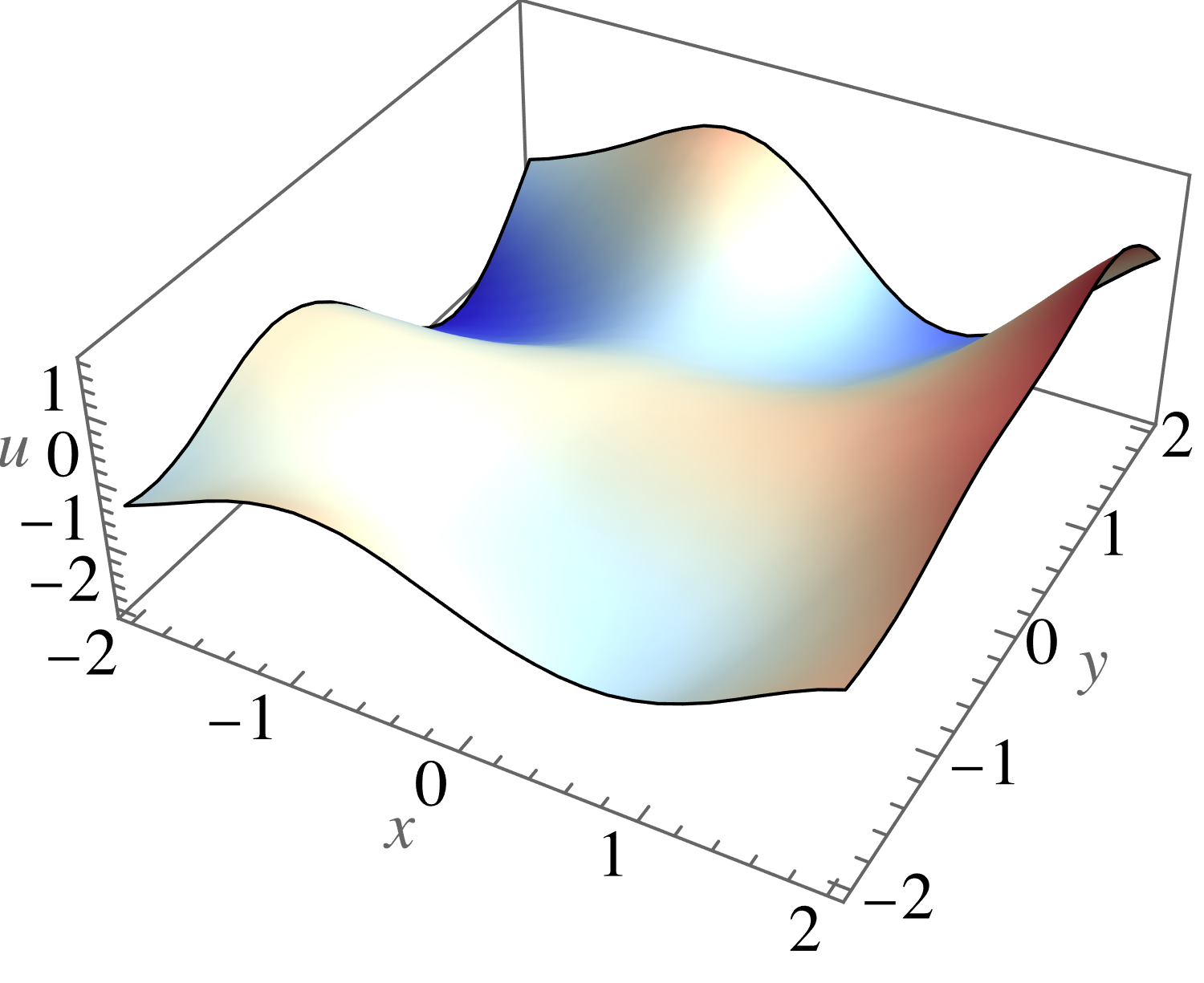
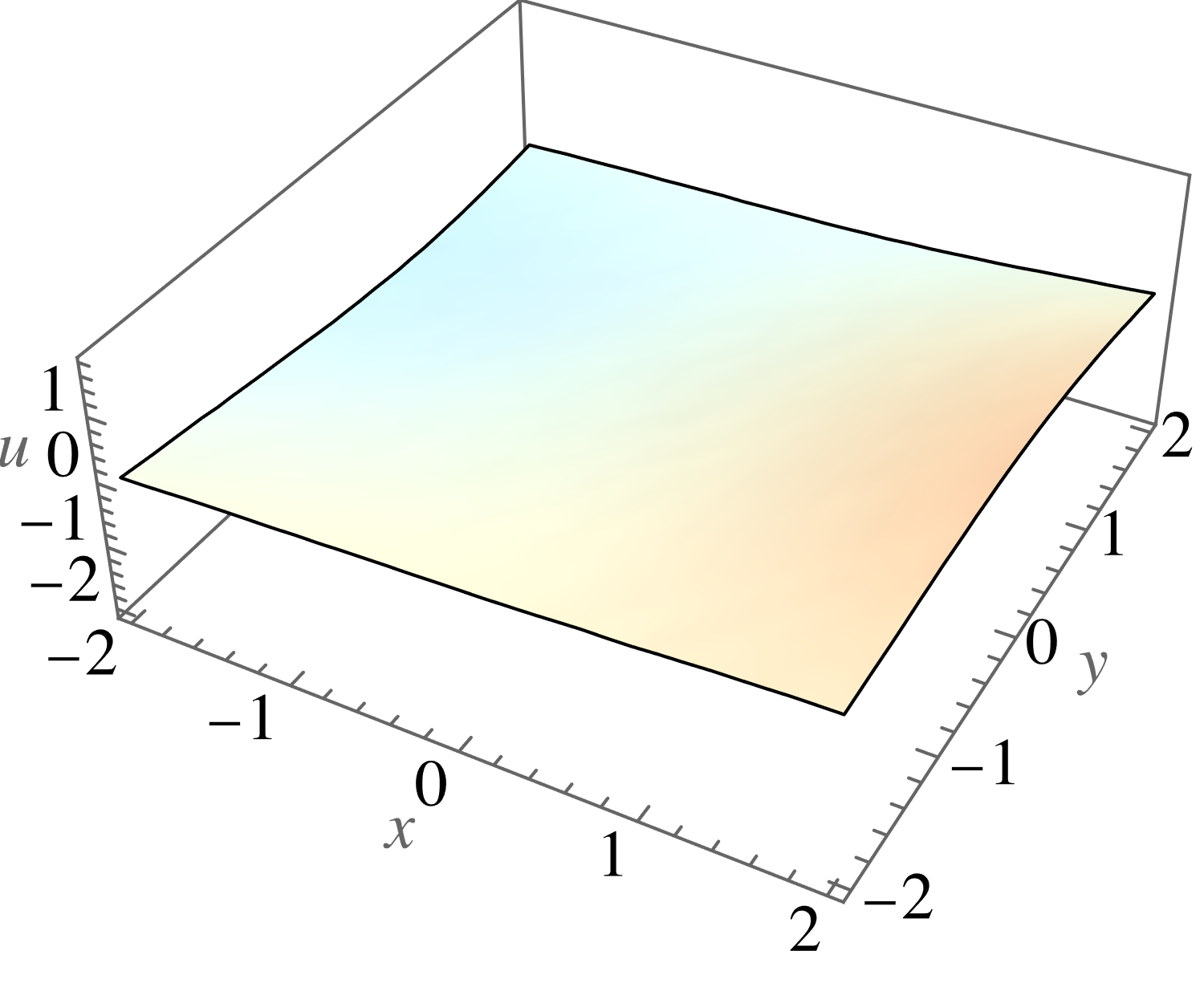
\displaystyle\frac{\partial f_{1}}{\partial x_{1}}-\frac{\partial^{3}f_{2}}{\partial x_{1}^{2}\partial x_{2}}=\frac{\partial f_{1}}{\partial x_{2}}+f_{2}=-\frac{\partial f_{2}}{\partial x_{1}}+3\frac{\partial f_{2}}{\partial x_{2}}=0.

Its solutions are vector valued functions $f(x_{1},x_{2})=(f_{1}(x_{1},x_{2}),f_{2}(x_{1},x_{2}))^{T}$ . Another example is the 2 dimensional heat equation, where $A$ is the $1\times 1$ matrix $A=[\partial_{x}^{2}+\partial_{y}^{2}-\partial_{t}]$ . Its solutions are scalar functions $u(x,y,t)$ , such as the one displayed in Figure 1.

The famed Ehrenpreis-Palamodov fundamental principle asserts that all solutions to the PDEs represented by $A$ can be written as suitable integrals of exponential-polynomial solutions, each of which corresponds to roots and multiplicities of the polynomial module generated by rows of $A$ .

Theorem 3.1.

(Ehrenpreis 1970; Palamodov 1970; Hörmander 1990; Björk 1979) Let $A\in R^{\ell\times{\ell^{\prime\prime}}}$ and let $\Omega\subseteq\mathbb{R}^{n}$ be a convex, compact set. There exist algebraic varieties $\{V_{1},\dotsc,V_{s}\}$ and ${\ell^{\prime\prime}}$ -tuples of polynomials $\{D_{i,1}(\mathbf{x},\mathbf{z}),\dotsc,D_{i,m_{i}}(\mathbf{x},\mathbf{z})\}_{i=1,\dotsc,s}$ such that any smooth solution $f\colon\Omega\to\mathbb{R}^{\ell^{\prime\prime}}$ to the equation $Af=0$ can be written as

\displaystyle f(\mathbf{x})

\displaystyle=\sum_{i=1}^{s}\sum_{j=1}^{m_{i}}\int_{V_{i}}D_{i,j}(\mathbf{x},\mathbf{z})e^{\langle\mathbf{x},\mathbf{z}\rangle}\,d\mu_{i,j}(\mathbf{z})

(2)

for a suitable choice of measures $\mu_{i,j}$ .

Following the terminology in (Cid-Ruiz et al. 2021; Cid-Ruiz & Sturmfels 2021), we call the polynomials $D_{i,j}(\mathbf{x},\mathbf{z})$ Noetherian multipliers. The Noetherian multipliers $D_{i,j}$ and varieties $V_{i}$ appearing in Theorem 3.1 can be computed algebraically; they are the higher-dimensional analogue of the roots and multiplicities of the characteristic polynomial. An algorithm for computing $D_{i,j}$ and $V_{i}$ is implemented under the command solvePDE in the Macaulay2 (Grayson & Stillman) package NotherianOperators (Chen et al. 2022b). A modern, algebraic and algorithmic treatment of linear PDEs with constant coefficients can be found in (Cid-Ruiz et al. 2021; Cid-Ruiz & Sturmfels 2021; Chen & Cid-Ruiz 2022; Ait El Manssour et al. 2021). We refer the interested reader to Appendix B for questions regarding convergence of the integrals in (2).

4 Gaussian Process Priors from the Ehrenpreis-Palamodov Theorem

We now construct GPs whose samples solve a system of linear PDEs $Af=0$ , using the Ehrenpreis-Palamodov fundamental principle, Theorem 3.1, as a blueprint. We set the mean function to zero, so our task, by Lemma 2.1, will be to find a covariance function that satisfies the PDEs in both the $\mathbf{x}$ and $\mathbf{x}^{\prime}$ arguments. The varieties $V_{i}$ and polynomials $D_{i,j}$ in Equation 2 can be computed algorithmically (Chen et al. 2022b; Cid-Ruiz et al. 2021; Cid-Ruiz & Sturmfels 2021; Chen & Cid-Ruiz 2022; Ait El Manssour et al. 2021), so what remains is to choose the measures $\mu_{i,j}$ , each supported on the variety $V_{i}$ .

We propose two approaches for choosing the measures. In the first one, coined Ehrenpreis-Palamodov Gaussian Process (EPGP), the $\mu_{i,j}$ are chosen to be Gaussian measures supported on the variety, with optional trainable length scale and shift parameters. This resembles the construction by Wilson & Adams 2013, but applied to Ehrenpreis-Palamodov integrals as opposed to Fourier transforms. Our second approach, Sparse EPGP (S-EPGP), chooses $\mu_{i,j}$ to be linear combinations of Dirac delta measures, whose locations and weights are learned. See (Lázaro-Gredilla et al. 2010) for a similar approach applied to Fourier transforms.

Before describing our covariance functions, we discuss the question of how to integrate over an algebraic variety. In certain cases our variety has a polynomial parametrization, in which case the integral can easily be computed by substituting the parametrization in. For example if $V$ is the variety corresponding to the parabola $y=x^{2}$ , we can rewrite an integral $\int_{V}f(x,y)\,d\mu(x,y)$ over $V$ as $\int_{\mathbb{C}}f(x,x^{2})\,d\mu^{\prime}(x)$ .

However, most algebraic varieties $V$ do not have a parametrization. In these cases we construct a parametrization implicitly by solving equations. If for example the variety $V$ is the set of points $(x,y,z)$ where $x^{3}-y^{2}+z^{2}=0$ , we could solve for $z$ to get $z=\pm\sqrt{y^{2}-x^{3}}$ . Thus, an integral of the form $\int_{V}f(x,y,z)\,d\mu(x,y,z)$ can be rewritten as a sum $\int_{\mathbb{C}^{2}}f(x,y,\sqrt{y^{2}-x^{3}})\,d\mu_{1}(x,y)+\int_{\mathbb{C}^{2}}f(x,y,-\sqrt{y^{2}-x^{3}})\,d\mu_{2}(x,y)$ of integrals over $\mathbb{C}^{2}$ . This construction works for arbitrary varieties $V\subseteq\mathbb{C}^{n}$ and relies on results in algebraic dimension theory. We now cite the main results and refer to e.g. the textbook by Eisenbud 1995 for a comprehensive treatment.

Suppose we denote the coordinates of $\mathbb{C}^{n}$ by $z_{1},\dotsc,z_{n}$ . If $V$ has dimension $d$ , there is a set of $d$ independent variables, say $\mathbf{z}^{\prime}=(z_{1},\dotsc,z_{d})$ after reordering, on which the remaining variables $\mathbf{z}^{\prime\prime}=(z_{d+1},\dotsc,z_{n})$ depend algebraically. Thus for each choice of $\mathbf{z}^{\prime}\in\mathbb{C}^{d}$ , there is a finite number of $\mathbf{z}^{\prime\prime}\in\mathbb{C}^{n-d}$ such that $\mathbf{z}=(\mathbf{z}^{\prime},\mathbf{z}^{\prime\prime})\in V$ . We denote this set by $\mathcal{S}_{\mathbf{z}^{\prime}}:=\{\mathbf{z}\in V\colon(z_{1},\dotsc,z_{d})=\mathbf{z}^{\prime}\}$ . Using this notation, an integral $\int_{V}f(\mathbf{z})\,d\mu(\mathbf{z})$ over $V$ can now be rewritten as an integral $\int_{\mathbb{C}^{d}}\sum_{\mathbf{z}\in\mathcal{S}_{\mathbf{z}^{\prime}}}f(\mathbf{z})\,d\mu(\mathbf{z}^{\prime})$ over the much easier to handle affine space $\mathbb{C}^{d}$ , at the cost of changing the measure and splitting our integral into several pieces.

4.1 Ehrenpreis-Palamodov Gaussian Processes (EPGP)

Let $Af=0$ be a system of PDEs whose solutions are, by Ehrenpreis-Palamodov, of the form $\phi(\mathbf{x})=\sum_{j}\int_{V}D_{j}(\mathbf{x},\mathbf{z})e^{\langle\mathbf{x},\mathbf{z}\rangle}\,d\mu_{j}(\mathbf{x})$ . We define the EPGP kernel $k_{\mathrm{EPGP}}(\mathbf{x},\mathbf{x}^{\prime})$ by combining the Ehrenpreis-Palamodov representation in both inputs $\mathbf{x},\mathbf{x}^{\prime}$ , the above implicit parametrization of the integrals, and a Gaussian measure on the frequency space of the $\mathbf{z}$ . We construct one covariance kernel for each summand in $\phi(\mathbf{x})$ and sum them to get the EPGP kernel $k_{\mathrm{EPGP}}$ :

$\displaystyle\Psi(\mathbf{x},\mathbf{z}^{\prime})$	$\displaystyle:=\sum_{j}\sum_{\mathbf{z}\in\mathcal{S}_{\mathbf{z}^{\prime}}}D_{j}(\mathbf{x},\mathbf{z})e^{\langle\mathbf{x},\mathbf{z}\rangle}$
$\displaystyle k_{\mathrm{EPGP}}(\mathbf{x},\mathbf{x}^{\prime})$	$\displaystyle:=$	(3)
	$\displaystyle\hskip-20.00003pt\int_{\mathbf{z}^{\prime}\in\sqrt{-1}\mathbb{R}^{d}}\Psi(\mathbf{x},\mathbf{z}^{\prime})\Psi(\mathbf{x}^{\prime},\mathbf{z}^{\prime})^{H}e^{-\frac{\\|\mathbf{z}^{\prime}\\|^{2}}{2}}\,d\mathcal{L}(\mathbf{z}^{\prime}).$

Here the superscript $H$ denotes the Hermitian transpose and $\mathcal{L}$ is the usual Lebesgue measure. We note that the integral may not converge everywhere, but we can introduce a shifting term to enforce convergence in any compact set $\Omega$ . See Appendix B for details. It is straightforward to check that $k_{\mathrm{EPGP}}(\mathbf{x},\mathbf{x}^{\prime})$ satisfies the PDEs in $A$ and the Hermitian transpose ensures that $k_{\mathrm{EPGP}}$ is positive semidefinite. A strictly real valued GP is obtained by taking the real part of $k_{\mathrm{EPGP}}$ .

In (3), we replaced the integral over the complex space $\mathbf{z}^{\prime}\in\mathbb{C}^{d}$ by an integral over purely imaginary vectors $\mathbf{z}^{\prime}\in\sqrt{-1}\mathbb{R}^{d}$ . This leads to more stationary kernels and we further motivate this choice and the choice of the Gaussian measure, in three examples:

Example 4.1 (No PDE).

If we impose no PDE constraints, we have $A=0$ , one variety $V=\mathbb{C}^{n}$ and one Noetherian multiplier $D(\mathbf{x},\mathbf{z})=1$ . So equation (3) becomes

	$\displaystyle k_{\mathrm{EPGP}}(\mathbf{x},\mathbf{x}^{\prime})$	$\displaystyle=\int_{\mathbf{z}\in\mathbb{R}}e^{\sqrt{-1}\langle\mathbf{x}-\mathbf{x}^{\prime},\mathbf{z}\rangle}e^{-\frac{\\|\mathbf{z}\\|^{2}}{2}}\,d\mathcal{L}(\mathbf{z})$
		$\displaystyle=\left(\sqrt{2\pi}\right)^{n}e^{-\frac{\\|\mathbf{x}-\mathbf{x}^{\prime}\\|^{2}}{2}}$

Thus, without PDEs, the EPGP kernel is the squared-exponential kernel, up to a constant scaling factor.

The discussion in this example extends to any system of PDEs $A$ whose characteristic variety $V$ is an affine subspace of $\mathbb{C}^{n}$ . For details, refer to Appendix G, cf. also (Lange-Hegermann 2021). ∎

Example 4.2 (Heat equation).

Let $A(\partial_{x},\partial_{t})=\partial_{x}^{2}-\partial_{t}$ be the one-dimensional heat equation. If we let $z_{1},z_{2}$ correspond to $\partial_{x},\partial_{t}$ respectively, the variety $V$ is given by $z_{1}^{2}=z_{2}$ and the sole Noetherian multiplier is $D=1$ . The EPGP kernel is defined when $t+t^{\prime}>-\frac{1}{2}$ , in which case we have

	$\displaystyle k_{\mathrm{EPGP}}(x,t;x^{\prime},t^{\prime})$	$\displaystyle=\int_{z\in\mathbb{R}}e^{\sqrt{-1}(x-x^{\prime})}e^{-z^{2}(t+t^{\prime})}e^{-\frac{z^{2}}{2}}\,d\mathcal{L}(z)$
		$\displaystyle=\sqrt{2\pi}\frac{e^{-\frac{(x-x^{\prime})^{2}}{2(1+2(t+t^{\prime}))}}}{\sqrt{1+2(t+t^{\prime})}}$

Here, integrating over $\sqrt{-1}\mathbb{R}$ as opposed to $\mathbb{C}$ removes unphysical solutions to the heat equation, such as $\phi(x,t)=e^{x+t}$ where heat increases exponentially with time.

This covariance function is the squared exponential covariance w.r.t. the space dimension at each fixed pair of times $(t,t^{\prime})$ . With increasing time, the scaling of the covariance shrinks resp. the length scales increase. We interpret this as heat going back to the mean value resp. being more smoothly distributed over time. ∎

Example 4.3 (Wave equation).

Let $A(\partial_{x},\partial_{t})=\partial_{x}^{2}-\partial_{t}^{2}$ be the 1-dimensional wave equation. The variety here is the set $z_{1}^{2}-z_{2}^{2}=0$ , which is the union of the lines $z_{1}=z_{2}$ and $-z_{1}=z_{2}$ . Thus we have $V_{j}=V(z_{1}+(-1)^{j}z_{2})$ and $D_{j}=1$ for $j=1,2$ . The EPGP kernel is equal to

	$\displaystyle\begin{split}k_{\mathrm{EPGP}}(x,t;x^{\prime},t^{\prime})=\int_{z\in\mathbb{R}}\left(e^{\sqrt{-1}z(x-t)}+e^{\sqrt{-1}z(x+t)}\right)\cdot\\ \left(e^{-\sqrt{-1}z(x^{\prime}-t^{\prime})}+e^{\sqrt{-1}z(x^{\prime}+t^{\prime})}\right)e^{-\frac{z^{2}}{2}}\,d\mathcal{L}(z)\end{split}$
	$\displaystyle\begin{split}=\sqrt{2\pi}\bigl(e^{-\frac{((x-t)-(x^{\prime}-t^{\prime}))^{2}}{2}}+e^{-\frac{((x-t)-(x^{\prime}+t^{\prime}))^{2}}{2}}+\\ e^{-\frac{((x+t)-(x^{\prime}-t^{\prime}))^{2}}{2}}+e^{-\frac{((x+t)-(x^{\prime}+t^{\prime}))^{2}}{2}}\bigr)\end{split}$

Here our choice of restricting to integrals over strictly imaginary numbers $\sqrt{-1}\mathbb{R}$ gets rid of non-stable solutions to the wave equations, such as $e^{x+t}$ .

While $k_{\mathrm{EPGP}}$ has four summands, we can also consider kernels with fewer summands. E.g.

\displaystyle k_{2}(x,t;x^{\prime},t^{\prime})=e^{-\frac{((x+t)-(x^{\prime}+t^{\prime}))^{2}}{2}}+e^{-\frac{((x-t)-(x^{\prime}-t^{\prime}))^{2}}{2}},

yields the covariance kernel of the GP $\phi_{1}(x+t)+\phi_{2}(x-t)$ , where $\phi_{1},\phi_{2}\sim GP(0,e^{-\frac{(x-x^{\prime})^{2}}{2}})$ . This is kernel in fact covers all smooth solutions to the 1-D wave equation, as d’Alembert discovered in 1747 (d’Alembert 1747) that all solutions are superpositions of waves travelling in opposite directions. ∎

Here we have tacitly assumed that the Ehrenpreis-Palamodov integral requires only one variety $V$ , i.e. $s=1$ . In the general case $s>1$ , we repeat the above construction for each variety $V_{i}$ and finally sum the resulting $s$ kernels.

We note that we may also parametrize the Gaussian measure imposed in Equation 3, for example with mean and scale parameters. By replacing $\exp(-\frac{\|\mathbf{z}^{\prime}\|^{2}}{2})$ by e.g. $\exp(-\sum_{i=1}^{d}\frac{(z_{i}-\mu_{i})^{2}}{2\sigma_{i}^{2}})$ , we obtain a family of EPGP kernels, which we can train on given data to find the parameters $\mu_{i},\sigma^{2}_{i}$ maximizing the log-marginal likelihood. In the case of no PDE constraints, we recover exactly the covariance kernels proposed in (Wilson & Adams 2013). In Figure 3 of Section 6.1 we investigate the effect of a scale parameter in the posterior distribution of a solution to the 2 dimensional heat equation.

4.2 Sparse Ehrenpreis-Palamodov Gaussian Processes (S-EPGP)

Instead of imposing the measure $e^{-\|\mathbf{z}^{\prime}\|^{2}/2}\,d\mathcal{L}(\mathbf{z}^{\prime})$ in our kernel, we outline a computationally efficient method for estimating the integral by a weighted sum. The kernels described in this section resemble the ones in (Lázaro-Gredilla et al. 2010), but using representations of PDE solutions via the Ehrenpreis-Palamodov fundamental principle as opposed to the Fourier transform. For notational simplicity we assume that the $D_{j}(\mathbf{x},\mathbf{z})$ are scalar valued and there is only one variety in Equation 2, i.e. $s=1$ ; the extension of our analysis to the general case is straight forward and a concrete example of S-EPGP applied to Maxwell’s equations can be seen in Section 6.3.

The idea is to choose the measures $\mu_{i,j}$ in Equation 2 as linear combinations of Dirac “delta functions”. Ideally we would define a GP prior with realizations of the form

\displaystyle f(\mathbf{x})=\sum_{j=1}^{m}\sum_{i=1}^{r}w_{i,j}D_{j}(\mathbf{x},\mathbf{z}_{i,j})e^{\langle\mathbf{x},\mathbf{z}_{i,j}\rangle},

where all $z_{i,j}\in V$ . This is precisely the Ehrenpreis-Palamodov representation of solutions, as in equation 2, with $r$ Dirac delta measures for each integral. Given training data, we would then choose $\mathbf{z}_{i,j}\in V$ as to maximize the log marginal likelihood. Unfortunately, the requirement for $\mathbf{z}_{i,j}$ to lie on an algebraic variety makes it challenging to directly use a gradient descent based optimization method.

Instead, we use the implicit parametrization trick from the beginning of this section and are looking at a GP with realizations of the form

	$\displaystyle f(\mathbf{x})$	$\displaystyle=\sum_{j=1}^{m}\sum_{i=1}^{r}w_{i,j}\frac{1}{\|S_{\mathbf{z}^{\prime}_{i,j}}\|}\left(\sum_{\mathbf{z}\in S_{\mathbf{z}^{\prime}_{i,j}}}D_{j}(\mathbf{x},\mathbf{z})e^{\langle\mathbf{x},\mathbf{z}\rangle}\right)$
		$\displaystyle=:\mathbf{w}^{T}\mathbf{\phi}(\mathbf{x}),$

where now $\mathbf{z}^{\prime}_{i,j}\in\mathbb{C}^{d}$ , $d=\dim V$ , and $\mathbf{w},\mathbf{\phi}(x)$ are both vectors of length $mr$ . For the same reasons as in the previous section we may also choose $\mathbf{z}^{\prime}_{i,j}\in\sqrt{-1}\mathbb{R}^{d}$ . To turn $f(\mathbf{x})$ into a GP, set $w_{i,j}\sim\mathcal{N}\left(0,\frac{1}{mr}\Sigma\right)$ , where $\Sigma$ is a diagonal matrix with positive entries $\sigma_{i}^{2}$ for $i=1,\dotsc,mr$ . We then get a covariance function of the form

\displaystyle k_{\mathrm{S-EPGP}}(\mathbf{x},\mathbf{x}^{\prime})=\frac{1}{mr}\mathbf{\phi}(\mathbf{x})^{H}\Sigma\mathbf{\phi}(\mathbf{x}^{\prime})

(4)

where $\mathbf{\phi}(\mathbf{x})^{H}$ denotes the conjugate transpose of $\mathbf{\phi}(\mathbf{x})$ . Refer to Appendix C for details regarding the S-EPGP objective function and inference. An example implementation in PyTorch can be found in Appendix H.

4.3 Summary

Below, we summarize concrete steps required to constuct (S-)EPGP kernels. We emphasize every step can be implemented algorithmically, given a system of PDEs as input.

1.

Use the Macaulay2 command solvePDE to compute the varieties $V_{i}$ and Noetherian multipliers.
2.

Find nice parametrizations $\mathbb{C}^{d}\to V_{i}$ for each variety. If such a parametrization does not exist, use a combination of a random linear change of coordinates and a univariate polynomial solver.
3.

Compute the resulting integral (3). If a closed form solution exists, use it as-is to obtain an EPGP kernel. If not, use S-EPGP (4).

Note that EPGP can be Monte-Carlo approximated using the S-EPGP kernel with frozen, randomly selected $z_{i,j}$ parameters.

5 Comparison to the Literature

Physics informed methods are a central research topic in machine learning. The PINN approach adds additional loss terms for a deep neural network from the differential equations at collocation points, sometimes combined with feature engineering, specific network structures, usage of symmetries and similar techniques, see e.g. (van Milligen et al. 1995; Lagaris et al. 2000; Raissi et al. 2019; Cuomo et al. 2022; Drygala et al. 2022). Such techniques also include GPs as a tool, e.g. (Zhang et al. 2022) uses GPs to estimate solutions of a single PDE where the derivatives of the GPs are used in the loss function and (Chen et al. 2022a) uses GPs to model a single function constrained by a single linear PDE. Another recent approach uses GPs and collocation points to solve linear PDE systems with constant coefficients (Pförtner et al. 2022).

There are several other deep learning approaches to systems of PDEs. As an example, weak adversarial networks (Zang et al. 2020) strive for a Nash equilibrium between a neural network that minimizes a weak formulation for a PDE and a second neural network modeling the test function in this weak formulation. Alternatively, when given a variational formulation of a PDE, where the solution of the PDEs minimizes an integral, the deep Ritz method (Yu et al. 2018) approximates solutions of PDEs via a neural network such that a discrete approximation of the integral is minimized. Ordinary differential equations have been used to construct deep neural networks (Chen et al. 2018), which has in turn being used to learn differential equations (Saemundsson et al. 2020). See also the review (Tanyu et al. 2022) on similar deep learning methods.

The approaches in (Macêdo & Castro 2008; Scheuerer & Schlather 2012; Wahlström et al. 2013; Solin et al. 2018; Jidling et al. 2018; Särkkä 2011; Jidling et al. 2017; Lange-Hegermann 2018; Dong 1989; van den Boogaart 2001; Albert 2019) construct GPs for controllable systems of linear PDEs with constant coefficients using parametrizations and Lemma 2.1. In the language of our paper, the controllable systems are the systems with characteristic variety equal to the full space of frequencies, see Appendix G. In particular, the approaches in all of the above papers are special cases of our EPGPs. When we would apply EPGPs to the differential equations treated in these papers, we would get precisely the same results. However, none of these approaches can treat the three examples that we demonstrate in Section 6, as these examples all have proper characteristic varieties. Besginow & Lange-Hegermann 2022 construct priors for all systems of linear ODEs with constant coefficients by splitting apart the embedded components in the characteristic variety and model them via linear regression, whereas the controllable components are again parametrized. Again, this approach is a special case of EPGPs.

Several paper deal with special cases of controllable systems. The papers (Alvarez et al. 2009; Hartikainen & Sarkka 2012; Alvarez et al. 2013; Reece et al. 2014; Alvarado et al. 2014; Ghosh et al. 2015; Raissi et al. 2017; Camps-Valls et al. 2018; Särkkä et al. 2018; Nayek et al. 2019; Pang et al. 2019; Rogers et al. 2020; Gahungu et al. 2022) constructs priors for linear ODE or PDE systems with forcing terms, which are also controllable. Notably, (Ward et al. 2020) used these methods in the context of linearization. Furthermore, Ranftl 2022 uses GPs to construct neural networks which only allow approximate solutions to given PDEs as trained functions.

Figure 2: Comparison of the error between EPGP (ours) and PINN for learning a solution to a 1D heat equation. On the left, training data is constrained to

t=0

, which tests PDE solving capabilities based on initial data. On the right, training data is spread over the entire interval

t\in[0,5]

to test interpolation performance. EPGP yields considerably better results over a wide range of the amount of training data. The error regions stem from training the model on 10 different instances.

GPs are a classical tool for purely data based simulation models. Hence, they appear regularly with their standard covariance functions as an approximate model inside models connected to differential equations (Chai et al. 2008; Zhao et al. 2011; Bilionis et al. 2013; Klenske et al. 2015; Ulaganathan et al. 2016; Rai & Tripathi 2019; Chen et al. 2021). Furthermore, a huge class of probabilistic ODE solvers (Calderhead et al. 2009; Schober et al. 2014; Marco et al. 2015; Schober et al. 2019; Krämer & Hennig 2021; Tronarp et al. 2021; Bosch et al. 2021; Schmidt et al. 2021) and a smaller class of probabilistic PDE solvers (Bilionis 2016; Cockayne et al. 2017; Krämer et al. 2022) make use of GPs when dealing with non-linear differential equations, without constructing new covariance functions. For systems of PDEs, solutions can be propagated forward in time using numerical discretization combined with GPs (Raissi et al. 2018).

Differential equations are often used together with boundary conditions. There is recent interest in constructing GP priors encoding such boundary conditions (Tan 2018; Solin & Kok 2019; Gulian et al. 2022; Nicholson et al. 2022) and even work constructing GP priors combining differential equations with boundary conditions (Lange-Hegermann 2021; Lange-Hegermann & Robertz 2022).

6 Examples

We demonstrate (S-)EPGPs on three systems of PDEs and a fourth one in Appendix H. While the systems presented below are simple, they are all fundamental physical systems still subject to active research, in particular in the field of finite element methods (Steinbach & Zank 2019; Gopalakrishnan et al. 2017; Perugia et al. 2020). Due to their algebraic simplicity, we omit here details regarding the computation of their corresponding Noetherian multipliers and characteristic varieties.

We compare our method with a version of PINN (Raissi et al. 2019), implementing some of the recent improvements in the review paper by Cuomo et al. 2022.

We note that there were no previously known GP priors for any of these systems, as none of them are controllable.

The code used to generate figures and tables is available at

https://github.com/haerski/EPGP

Animated versions of some of the figures can be found on the expository website

https://mathrepo.mis.mpg.de/EPGP/

Copies of the codebase and animations can also be found in the ancillary files.

6.1 Heat equation

The one-dimensional heat equation is given by the PDE $\partial_{x}^{2}u(x,t)=\partial_{t}u(x,t)$ . Our first goal is to infer an exact solution purely from sampled data points, without any knowledge about boundary conditions. Consider the domain $(x,t)\in[-5,5]\times[0,5]$ on a $101\times 51$ grid of equally spaced points. These 5151 corresponding function values serve as our “underlying truth”.

We compare our method with PINN (Raissi et al. 2019) in two setups. First, we test the ability of the model to solve the heat equation given initial data. Therefore, we train on different numbers of randomly chosen points at $t=0$ and study the mean square error over all time points $t\in[0,5]$ . In our second setup, we test the ability of the model to interpolate the underlying true solution from a limited set of data scattered throughout time. We train on different numbers of points chosen uniformly at random over the $101\times 51$ grid. The results are depicted in Figure 2. The GP achieves an error several orders of magnitude smaller than the errors of PINN, even with fewer data points. In addition, there is a drastic difference in total computation time between EPGP (10s) and PINN (2h) using an Nvidia A100 GPU.

Next, we apply the EPGP to the 2D heat equation, with an added scale parameter on the Gaussian measure as discussed in the end of Section 4.1. The initial data is given at $t=0$ , on a $101\times 101$ grid in the square $[-5,5]^{2}$ , where every value is equal to 0, except for a region depicting a smiling face where we set the value to 1. In this case, the scaling factor $\sigma^{2}$ in the covariance kernel determines how strongly the initial data is respected. Figure 3 compares the posterior mean at fives timepoints. When $\sigma^{2}=20$ , the prior allows abrupt changes and the inferred function conforms to the jagged edges in the data. In contrast, for $\sigma^{2}=2$ the prior prefers smooth interpretations of the initial data. In both cases we show the instantaneous smoothing behavior at times $t>0$ , which is characteristic to solutions of the heat equation. For details (covariance functions, experimental setup, etc.) and additional comparisons about the heat equation see Appendix D.

6.2 2D wave equation

Consider the 2D wave equation, given by $\frac{\partial^{2}z}{\partial x^{2}}+\frac{\partial^{2}z}{\partial y^{2}}=\frac{\partial^{2}z}{\partial t^{2}}$ . The solution we are trying to learn is obtained by solving the wave equation numerically, subject to boundary conditions $z(0,y,t)=z(1,y,t)=z(x,0,t)=z(x,1,t)=0$ , and initial conditions $z(x,y,0)=\sin(4\pi x)y(1-y)$ , and $\frac{\partial z}{\partial t}(x,y,0)=0$ . A plot of the numerical solution can be found on the top row of Figure 4. The recent theoretical papers (Henderson et al. 2023a; Henderson et al. 2023b) construct and study a covariance function for the 3D wave equation with initial conditions at $t=0$ .

To learn the numerical solution, we split the domain $(x,y,t)\in[0,1]^{3}$ into a $21\times 21\times 21$ grid and use the data at $t=0,0.05,0.1$ for training. For S-EPGP, we use a sum of 16 Dirac delta kernels, whose positions we learn. A PINN model, with 15 hidden layers of size 200, was also trained on the same data, but failed to get adequate extrapolation performance. The bottom row of Figure 4 contains a PINN instance trained for 200,000 epochs. Technical details about wave equation, our experimental setup, and an additional comparison of (S-)EPGP models can be found in Appendix E. An example animation of colliding 2-dimensional wavefronts can be found in the file crashing_waves.mp4, provided as an ancillary file.

Table 1: Root mean square errors learning an exact solution to Maxwell’s equations, using different number of datapoints for training. Top: S-EPGP, with a varying number of Dirac delta measures. Bottom: PINN. Here HLW stands for “hidden layer width”. Each experiment is repeated 10 times

Deltas	5 datapoints	10 datapoints	50 datapoints	100 datapoints	1000 datapoints
$24$	$6.08\pm 0.797$	$8.92\pm 1.87$	$1.38\pm 0.698$	$0.981\pm 0.361$	$0.884\pm 0.347$
$48$	$4.31\pm 0.431$	$6.98\pm 1.37$	$0.356\pm 0.392$	$0.11\pm 0.101$	$0.0298\pm 0.0295$
$96$	$4.21\pm 0.387$	$3.81\pm 0.747$	$0.173\pm 0.169$	$0.00521\pm 0.00221$	$0.00192\pm 0.00203$
$192$	$3.9\pm 0.302$	$3.21\pm 0.706$	$1.22\pm 0.696$	$0.027\pm 0.0291$	$0.00239\pm 0.00155$
$384$	$\mathbf{3.45\pm 0.364}$	$\mathbf{2.4\pm 0.796}$	$\mathbf{0.192\pm 0.193}$	$\mathbf{0.00974\pm 0.0113}$	$\mathbf{0.000469\pm 0.00017}$
HLW	5 datapoints	10 datapoints	50 datapoints	100 datapoints	1000 datapoints
$50$	$4.71\pm 0.403$	$4.09\pm 0.781$	$1.05\pm 0.304$	$0.742\pm 0.36$	$0.1\pm 0.0415$
$100$	$4.63\pm 0.469$	$4.12\pm 0.783$	$1.03\pm 0.278$	$0.693\pm 0.31$	$0.0948\pm 0.0272$
$200$	$\mathbf{4.72\pm 0.42}$	$\mathbf{4.1\pm 0.789}$	$\mathbf{1.06\pm 0.281}$	$\mathbf{0.73\pm 0.296}$	$\mathbf{0.0924\pm 0.0237}$

6.3 Maxwell’s equations

The homogeneous Maxwell equations in a vacuum are

	$\displaystyle\nabla\cdot\mathbf{E}$	$\displaystyle=0$	$\displaystyle\nabla\times\mathbf{E}$	$\displaystyle=-\frac{\partial\mathbf{B}}{\partial t}$
	$\displaystyle\nabla\cdot\mathbf{B}$	$\displaystyle=0$	$\displaystyle\qquad\nabla\times\mathbf{B}$	$\displaystyle=\frac{\partial\mathbf{E}}{\partial t},$

where $\mathbf{E}=(E_{x}(x,y,z,t),E_{y}(x,y,z,t),E_{z}(x,y,z,t))^{T}$ is the vector field corresponding to the electric field and $\mathbf{B}=(B_{x}(x,y,z,t),B_{y}(x,y,z,t),B_{z}(x,y,z,t))^{T}$ is the vector field corresponding to the magnetic field.

We run the S-EPGP algorithm using $m=4,8,16,32$ , and $64$ Dirac delta measures for each of the six multipliers. For comparison, we repeat the experiment with PINN, where we base hyperparameters on (Mathews et al. 2021) and report the results in Table 1. For details about Noetherian multipliers, the characteristic variety and implementation of S-EPGP and PINN see Appendix F.

The S-EPGP method learns the true underlying solution much better than PINN, achieving errors several orders of magnitude smaller even with a relatively small number of Dirac delta measures. Runtimes for S-EPGP scale well and outperform PINN. Our fastest S-EPGP model, with 24 Dirac deltas trained on only 5 points, completes 10000 training epochs in about 60 seconds on an Nvidia A100 GPU, whereas the slowest one, with 384 Dirac deltas trained on 1000 points, takes about 70 seconds to complete 10000 epochs. In comparison, each PINN model took about 200 seconds to complete 10000 epochs on the same GPU.

For an example using EPGP for generating solutions to Maxwell’s equations, see the ancillary files maxwell_E.mp4 and maxwell_B.mp4.

7 Discussion

Our method takes a starkly different approach to solving and learning PDEs compared to other physics informed machine learning methods such as PINN. As is common in applied non-linear algebra (Michalek & Sturmfels 2021), our philosophy is to remain in the exact setting as much as possible. This is evidenced by the application of exact symbolic algebraic techniques and the Ehrenpreis-Palamodov Fundamental Principle in the construction of our kernels. Thus we say that (S-)EPGP is physics constrained, as all realizations from our GPs are, by construction, exact solutions to the PDE system. Being constrained to solutions is not necessarily a disadvantage when dealing with noisy data, or even data that does not properly follow the PDEs. The usual GP approaches account for such scenarios by including additional components to the covariance function. Our experiments show the exact approach to be the superior and scalable, in both interpolation (learning) and extrapolation (solving) tasks. Non-exactness in the form of noise is only introduced at the very last step as we formulate the GP, which — unlike PINN— makes the (S-)EPGP training objective statistically well motivated and enables the usage of well-established techniques for sparse, variational, and approximate GPs. Furthermore, our method removes the hyperparameter required for tuning PINN’s multiple loss functions.

Compared to other methods of learning and solving PDEs, our method is also completely data-driven and algorithmic. We do not for example distinguish the time dimension from other spacial dimensions, as is often done in numerical methods. Our method also does not require explicit initial and boundary conditions: data points can be given anywhere in the domain and can consist of function values, derivatives, or any combination thereof. For vector-valued functions, we can also learn on partial representations of the data, for example using just electric field data to learn a solution to Maxwell’s equations in order to infer the corresponding magnetic field. This makes (S-)EPGP extremely flexible and applicable with minimal domain expertise.

Acknowledgements

The second author acknowledges the support of the SAIL network, funded by the Ministerium für Kultur und Wissenschaft of the state Nordrhein-Westfalen in Germany.

The authors thank the organizers of the “Workshop on Differential Algebra” in June 2022 at MPI MiS, Leipzig Germany, for providing the perfect atmosphere to start this research.

The authors thank the anonymous referees for carefully reading the manuscript and offering insightful comments and suggestions which improved the paper overall.

References

Ait El Manssour et al. (2021) Ait El Manssour, R., Härkönen, M., and Sturmfels, B. Linear PDE with constant coefficients. Glasgow Mathematical Journal, 2021.
Albert (2019) Albert, C. G. Gaussian processes for data fulfilling linear differential equations. Multidisciplinary Digital Publishing Institute Proceedings, 2019.
Alvarado et al. (2014) Alvarado, P. A., Alvarez, M. A., Daza-Santacoloma, G., Orozco, A., and Castellanos-Dominguez, G. A latent force model for describing electric propagation in deep brain stimulation: A simulation study. In 2014 International Conference of the IEEE Engineering in Medicine and Biology Society, 2014.
Alvarez et al. (2009) Alvarez, M., Luengo, D., and Lawrence, N. D. Latent force models. In AISTATS, 2009.
Alvarez et al. (2013) Alvarez, M. A., Luengo, D., and Lawrence, N. D. Linear latent force models using gaussian processes. IEEE transactions on pattern analysis and machine intelligence, 2013.
Berns et al. (2020) Berns, F., Lange-Hegermann, M., and Beecks, C. Towards Gaussian processes for automatic and interpretable anomaly detection in industry 4.0. In Proceedings of the International Conference on Innovative Intelligent Industrial Production and Logistics – IN4PL, 2020.
Besginow & Lange-Hegermann (2022) Besginow, A. and Lange-Hegermann, M. Constraining Gaussian Processes to Systems of Linear Ordinary Differential Equations. In NeurIPS. 2022.
Bilionis (2016) Bilionis, I. Probabilistic solvers for partial differential equations. arXiv:1607.03526, 2016.
Bilionis et al. (2013) Bilionis, I., Zabaras, N., Konomi, B. A., and Lin, G. Multi-output separable Gaussian process: Towards an efficient, fully Bayesian paradigm for uncertainty quantification. Journal of Computational Physics, 2013.
Björk (1979) Björk, J.-E. Rings of differential operators. North-Holland Mathematical Library. 1979.
Bogachev (1998) Bogachev, V. I. Gaussian measures. Number 62. American Mathematical Soc., 1998.
Bosch et al. (2021) Bosch, N., Hennig, P., and Tronarp, F. Calibrated adaptive probabilistic ODE solvers. In AISTATS, 2021.
Calderhead et al. (2009) Calderhead, B., Girolami, M., and Lawrence, N. D. Accelerating Bayesian inference over nonlinear differential equations with Gaussian processes. NeurIPS, 2009.
Camps-Valls et al. (2018) Camps-Valls, G., Martino, L., Svendsen, D. H., Campos-Taberner, M., Muñoz-Marí, J., Laparra, V., Luengo, D., and García-Haro, F. J. Physics-aware gaussian processes in remote sensing. Applied Soft Computing, 2018.
Chai et al. (2008) Chai, K., Williams, C., Klanke, S., and Sethu, V. Multi-task Gaussian process learning of robot inverse dynamics. NeurIPS, 2008.
Chen & Cid-Ruiz (2022) Chen, J. and Cid-Ruiz, Y. Primary decomposition of modules: a computational differential approach. Journal of Pure and Applied Algebra, 2022.
Chen et al. (2022a) Chen, J., Chen, Z., Zhang, C., and Jeff Wu, C. Apik: Active physics-informed kriging model with partial differential equations. SIAM/ASA Journal on Uncertainty Quantification, 2022a.
Chen et al. (2022b) Chen, J., Cid-Ruiz, Y., Härkönen, M., Krone, R., and Leykin, A. Noetherian operators in Macaulay2. J. Softw. Algebra Geom., 2022b.
Chen et al. (2018) Chen, R. T., Rubanova, Y., Bettencourt, J., and Duvenaud, D. K. Neural ordinary differential equations. NeurIPS, 31, 2018.
Chen et al. (2021) Chen, Y., Hosseini, B., Owhadi, H., and Stuart, A. M. Solving and learning nonlinear pdes with gaussian processes. Journal of Computational Physics, 2021.
Cid-Ruiz & Sturmfels (2021) Cid-Ruiz, Y. and Sturmfels, B. Primary decomposition with differential operators. arXiv:2101.03643, 2021.
Cid-Ruiz et al. (2021) Cid-Ruiz, Y., Homs, R., and Sturmfels, B. Primary ideals and their differential equations. Found. Comput. Math., 2021.
Cockayne et al. (2017) Cockayne, J., Oates, C., Sullivan, T., and Girolami, M. Probabilistic numerical methods for pde-constrained bayesian inverse problems. In AIP Conference Proceedings, volume 1853, 2017.
Cuomo et al. (2022) Cuomo, S., Di Cola, V. S., Giampaolo, F., Rozza, G., Raissi, M., and Piccialli, F. Scientific machine learning through physics-informed neural networks: Where we are and what’s next. arXiv:2201.05624, 2022.
d’Alembert (1747) d’Alembert, J. l. R. Recherches sur la courbe que forme une corde tendue mise en vibration. Memoires de l’Academie royale des sciences et belles lettres. Classe de mathematique., 3:214–219, 1747.
Dong (1989) Dong, A. Kriging variables that satisfy the partial differential equation $\delta$ z= y. In Geostatistics. 1989.
Drygala et al. (2022) Drygala, C., Winhart, B., di Mare, F., and Gottschalk, H. Generative modeling of turbulence. Physics of Fluids, 2022.
Duvenaud (2014) Duvenaud, D. Automatic model construction with Gaussian processes. PhD thesis, University of Cambridge, 2014.
Ehrenpreis (1970) Ehrenpreis, L. Fourier analysis in several complex variables. Wiley, 1970.
Eisenbud (1995) Eisenbud, D. Commutative algebra. Springer, 1995.
Gahungu et al. (2022) Gahungu, P., Lanyon, C. W., Alvarez, M. A., Bainomugisha, E., Smith, M., and Wilkinson, R. D. Adjoint-aided inference of gaussian process driven differential equations. NeurIPS, 2022.
Ghosh et al. (2015) Ghosh, S., Reece, S., Rogers, A., Roberts, S., Malibari, A., and Jennings, N. R. Modeling the thermal dynamics of buildings: A latent-force-model-based approach. ACM Transactions on Intelligent Systems and Technology, 2015.
Gopalakrishnan et al. (2017) Gopalakrishnan, J., Schöberl, J., and Wintersteiger, C. Mapped tent pitching schemes for hyperbolic systems. SIAM Journal on Scientific Computing, 39(6):B1043–B1063, 2017.
(34) Grayson, D. R. and Stillman, M. E. Macaulay2, a software system for research in algebraic geometry. Available at http://www.math.uiuc.edu/Macaulay2/.
Gulian et al. (2022) Gulian, M., Frankel, A., and Swiler, L. Gaussian process regression constrained by boundary value problems. Comput. Methods Appl. Mech. Engrg., 2022.
Härkönen (2022) Härkönen, M. Dual representations of polynomial modules with applications to partial differential equations. PhD thesis, Georgia Institute of Technology, 2022.
Harrington et al. (2016) Harrington, H. A., Ho, K. L., and Meshkat, N. Differential algebra for model comparison. 2016. arXiv:1603.09730.
Hartikainen & Sarkka (2012) Hartikainen, J. and Sarkka, S. Sequential inference for latent force models. arXiv:1202.3730, 2012.
Henderson et al. (2023a) Henderson, I., Noble, P., and Roustant, O. Characterization of the second order random fields subject to linear distributional pde constraints. arXiv:2301.06895, 2023a.
Henderson et al. (2023b) Henderson, I., Noble, P., and Roustant, O. Wave equation-tailored Gaussian process regression with applications to related inverse problems. hal-03941939, 2023b.
Hernández Rodríguez et al. (2022) Hernández Rodríguez, T., Sekulic, A., Lange-Hegermann, M., and Frahm, B. Designing robust biotechnological processes regarding variabilities using multi-objective optimization applied to a biopharmaceutical seed train design. Processes, 2022.
Hörmander (1990) Hörmander, L. An introduction to complex analysis in several variables. North-Holland Mathematical Library. Third edition, 1990.
Jidling et al. (2017) Jidling, C., Wahlström, N., Wills, A., and Schön, T. B. Linearly Constrained Gaussian Processes. In NeurIPS, 2017.
Jidling et al. (2018) Jidling, C., Hendriks, J., Wahlström, N., Gregg, A., Schön, T. B., Wensrich, C., and Wills, A. Probabilistic Modelling and Reconstruction of Strain. Nuclear Instruments and Methods in Physics Research Section B: Beam Interactions with Materials and Atoms, 2018.
Klenske et al. (2015) Klenske, E. D., Zeilinger, M. N., Schölkopf, B., and Hennig, P. Gaussian process-based predictive control for periodic error correction. IEEE Transactions on Control Systems Technology, 2015.
Krämer & Hennig (2021) Krämer, N. and Hennig, P. Linear-time probabilistic solution of boundary value problems. NeurIPS, 2021.
Krämer et al. (2022) Krämer, N., Schmidt, J., and Hennig, P. Probabilistic numerical method of lines for time-dependent partial differential equations. In AISTATS, 2022.
Lagaris et al. (2000) Lagaris, I. E., Likas, A. C., and Papageorgiou, D. G. Neural-network methods for boundary value problems with irregular boundaries. IEEE Transactions on Neural Networks, 2000.
Lange-Hegermann (2018) Lange-Hegermann, M. Algorithmic Linearly Constrained Gaussian Processes. In NeurIPS. 2018.
Lange-Hegermann (2021) Lange-Hegermann, M. Linearly constrained Gaussian processes with boundary conditions. In AISTATS, 2021.
Lange-Hegermann & Robertz (2022) Lange-Hegermann, M. and Robertz, D. On boundary conditions parametrized by analytic functions. In Computer Algebra in Scientific Computing, 2022.
Lázaro-Gredilla et al. (2010) Lázaro-Gredilla, M., Quiñnero-Candela, J., Rasmussen, C. E., and Figueiras-Vidal, A. R. Sparse spectrum gaussian process regression. JMLR, 2010.
Loshchilov & Hutter (2016) Loshchilov, I. and Hutter, F. SGDR: Stochastic gradient descent with warm restarts. arXiv:1608.03983, 2016.
Macêdo & Castro (2008) Macêdo, I. and Castro, R. Learning Divergence-free and Curl-free Vector Fields with Matrix-valued Kernels. Instituto Nacional de Matematica Pura e Aplicada, Brasil, Tech. Rep, 2008.
Marco et al. (2015) Marco, A., Hennig, P., Bohg, J., Schaal, S., and Trimpe, S. Automatic LQR tuning based on Gaussian process optimization: Early experimental results. In Second Machine Learning in Planning and Control of Robot Motion Workshop at International Conference on Intelligent Robots and Systems, 2015.
Mathews et al. (2021) Mathews, A., Francisquez, M., Hughes, J. W., Hatch, D. R., Zhu, B., and Rogers, B. N. Uncovering turbulent plasma dynamics via deep learning from partial observations. Phys. Rev. E, 2021.
Michalek & Sturmfels (2021) Michalek, M. and Sturmfels, B. Invitation to nonlinear algebra. Springer, 2021.
Nayek et al. (2019) Nayek, R., Chakraborty, S., and Narasimhan, S. A gaussian process latent force model for joint input-state estimation in linear structural systems. Mechanical Systems and Signal Processing, 2019.
Nicholson et al. (2022) Nicholson, J., Kiessler, P., and Brown, D. A. A kernel-based approach for modelling Gaussian processes with functional information. arXiv:2201.11023, 2022.
Palamodov (1970) Palamodov, V. P. Linear differential operators with constant coefficients. Springer, 1970.
Pang et al. (2019) Pang, G., Yang, L., and Karniadakis, G. E. Neural-net-induced gaussian process regression for function approximation and pde solution. Journal of Computational Physics, 2019.
Perugia et al. (2020) Perugia, I., Schöberl, J., Stocker, P., and Wintersteiger, C. Tent pitching and trefftz-dg method for the acoustic wave equation. Computers & Mathematics with Applications, 79(10):2987–3000, 2020.
Pförtner et al. (2022) Pförtner, M., Steinwart, I., Hennig, P., and Wenger, J. Physics-informed gaussian process regression generalizes linear pde solvers. arXiv:2212.12474, 2022.
Rai & Tripathi (2019) Rai, P. K. and Tripathi, S. Gaussian process for estimating parameters of partial differential equations and its application to the richards equation. Stochastic Environmental Research and Risk Assessment, 2019.
Raissi et al. (2017) Raissi, M., Perdikaris, P., and Karniadakis, G. E. Machine learning of linear differential equations using Gaussian processes. Journal of Computational Physics, 2017.
Raissi et al. (2018) Raissi, M., Perdikaris, P., and Karniadakis, G. E. Numerical gaussian processes for time-dependent and nonlinear partial differential equations. SIAM Journal on Scientific Computing, 2018.
Raissi et al. (2019) Raissi, M., Perdikaris, P., and Karniadakis, G. E. Physics-informed neural networks: A deep learning framework for solving forward and inverse problems involving nonlinear partial differential equations. Journal of Computational physics, 2019.
Rajput (1972a) Rajput, B. S. Gaussian measures on $\textup{L}^{p}$ spaces, $1\leq p<\infty$ . Journal of Multivariate Analysis, 2(4):382–403, 1972a.
Rajput (1972b) Rajput, B. S. On gaussian measures in certain locally convex spaces. Journal of Multivariate Analysis, 2(3):282–306, 1972b.
Rajput & Cambanis (1972) Rajput, B. S. and Cambanis, S. Gaussian processes and gaussian measures. The Annals of Mathematical Statistics, 43(6):1944–1952, 1972.
Ranftl (2022) Ranftl, S. A connection between probability, physics and neural networks. In Physical Sciences Forum. MDPI, 2022.
Rasmussen & Williams (2006) Rasmussen, C. E. and Williams, C. K. I. Gaussian processes for machine learning. MIT Press, Cambridge, MA, 2006.
Reece et al. (2014) Reece, S., Roberts, S., Ghosh, S., Rogers, A., and Jennings, N. R. Efficient state-space inference of periodic latent force models. JMLR, 2014.
Rogers et al. (2020) Rogers, T., Worden, K., and Cross, E. On the application of gaussian process latent force models for joint input-state-parameter estimation: With a view to bayesian operational identification. Mechanical Systems and Signal Processing, 2020.
Saemundsson et al. (2020) Saemundsson, S., Terenin, A., Hofmann, K., and Deisenroth, M. Variational integrator networks for physically structured embeddings. In AISTATS, 2020.
Särkkä (2011) Särkkä, S. Linear Operators and Stochastic Partial Differential Equations in Gaussian Process Regression. In ICANN. Springer, 2011.
Särkkä et al. (2018) Särkkä, S., Alvarez, M. A., and Lawrence, N. D. Gaussian process latent force models for learning and stochastic control of physical systems. IEEE Transactions on Automatic Control, 2018.
Scheuerer & Schlather (2012) Scheuerer, M. and Schlather, M. Covariance models for divergence-free and curl-free random vector fields. Stoch. Models, 2012.
Schmidt et al. (2021) Schmidt, J., Krämer, N., and Hennig, P. A probabilistic state space model for joint inference from differential equations and data. NeurIPS, 2021.
Schober et al. (2014) Schober, M., Duvenaud, D. K., and Hennig, P. Probabilistic ODE solvers with Runge-Kutta means. NeurIPS, 2014.
Schober et al. (2019) Schober, M., Särkkä, S., and Hennig, P. A probabilistic model for the numerical solution of initial value problems. Statistics and Computing, 2019.
Shankar (2019) Shankar, S. Controllability and vector potential: Six lectures at Steklov. arXiv:1911.01238, 2019.
Solin & Kok (2019) Solin, A. and Kok, M. Know your boundaries: Constraining Gaussian processes by variational harmonic features. In AISTATS. 2019.
Solin et al. (2018) Solin, A., Kok, M., Wahlström, N., Schön, T. B., and Särkkä, S. Modeling and Interpolation of the Ambient Magnetic Field by Gaussian Processes. IEEE Transactions on Robotics, 2018.
Steinbach & Zank (2019) Steinbach, O. and Zank, M. A stabilized space–time finite element method for the wave equation. In Advanced Finite Element Methods with Applications: Selected Papers from the 30th Chemnitz Finite Element Symposium 2017 30, pp. 341–370. Springer, 2019.
Steinruecken et al. (2019) Steinruecken, C., Smith, E., Janz, D., Lloyd, J., and Ghahramani, Z. The automatic statistician. In Automated Machine Learning. 2019.
Swain et al. (2016) Swain, P. S., Stevenson, K., Leary, A., Montano-Gutierrez, L. F., Clark, I. B., Vogel, J., and Pilizota, T. Inferring time derivatives including cell growth rates using gaussian processes. Nature communications, 2016.
Tan (2018) Tan, M. H. Y. Gaussian process modeling with boundary information. Statist. Sinica, 2018.
Tanyu et al. (2022) Tanyu, D. N., Ning, J., Freudenberg, T., Heilenkötter, N., Rademacher, A., Iben, U., and Maass, P. Deep learning methods for partial differential equations and related parameter identification problems. arXiv:2212.03130, 2022.
Thewes et al. (2015) Thewes, S., Lange-Hegermann, M., Reuber, C., and Beck, R. Advanced Gaussian Process Modeling Techniques. In Design of Experiments (DoE) in Powertrain Development, 2015.
Titsias (2009) Titsias, M. Variational learning of inducing variables in sparse gaussian processes. In AISTATS, 2009.
Tronarp et al. (2021) Tronarp, F., Särkkä, S., and Hennig, P. Bayesian ODE solvers: The maximum a posteriori estimate. Statistics and Computing, 2021.
Ulaganathan et al. (2016) Ulaganathan, S., Couckuyt, I., Dhaene, T., Degroote, J., and Laermans, E. Performance study of gradient-enhanced Kriging. Engineering with computers, 2016.
van den Boogaart (2001) van den Boogaart, K. G. Kriging for processes solving partial differential equations. In Proceedings of the Annual Conference of the International Association for Mathematical Geology, 2001.
van Milligen et al. (1995) van Milligen, B. P., Tribaldos, V., and Jiménez, J. Neural network differential equation and plasma equilibrium solver. Physical review letters, 1995.
Wahlström et al. (2013) Wahlström, N., Kok, M., Schön, T. B., and Gustafsson, F. Modeling Magnetic Fields using Gaussian Processes. In Proceedings of the 38th International Conference on Acoustics, Speech, and Signal Processing (ICASSP), 2013.
Ward et al. (2020) Ward, W., Ryder, T., Prangle, D., and Alvarez, M. Black-box inference for non-linear latent force models. In AISTATS, 2020.
Wilson & Adams (2013) Wilson, A. and Adams, R. Gaussian process kernels for pattern discovery and extrapolation. In ICML, 2013.
Yu et al. (2018) Yu, B. et al. The deep ritz method: a deep learning-based numerical algorithm for solving variational problems. Communications in Mathematics and Statistics, 2018.
Zang et al. (2020) Zang, Y., Bao, G., Ye, X., and Zhou, H. Weak adversarial networks for high-dimensional partial differential equations. Journal of Computational Physics, 2020.
Zhang et al. (2022) Zhang, J., Zhang, S., and Lin, G. Pagp: A physics-assisted gaussian process framework with active learning for forward and inverse problems of partial differential equations. arXiv:2204.02583, 2022.
Zhao et al. (2011) Zhao, H., Jin, R., Wu, S., and Shi, J. Pde-constrained gaussian process model on material removal rate of wire saw slicing process. Journal of Manufacturing Science and Engineering, 2011.
Zimmer et al. (2018) Zimmer, C., Meister, M., and Nguyen-Tuong, D. Safe active learning for time-series modeling with Gaussian processes. In NeurIPS, 2018.

Appendix A Proof of Lemma 2.1

Our proof hinges on the fact that Gaussian processes and Gaussian measures are essentially the same concepts when defined on reasonable function spaces. The pushforward property is then easy to check for Gaussian measures.

We will work with a space $\F$ of functions, which can be a general locally convex topological vector space (LCS), but for our purposes, we work with $\F=C^{\infty}(\Omega)$ endowed with the topology induced by the semi norms $p_{\alpha}(f)=\sup_{x\in\Omega}|\partial^{\alpha}f(x)|$ (recall here that we consider $\Omega$ to be the closure of an open, convex, bounded set). This topology induces the structure of a separable Fréchet space on $\F$ . We write $\F^{*}$ for the topological dual of $\F$ and $\delta_{x}\colon f\in\F\mapsto f(x)$ for the evaluation functionals. It turns out that $\delta_{x}$ span a dense set in $\F^{*}$ , a property which will be crucial in the sequel.

Lemma A.1.

Let $\F=C^{\infty}(\Omega)$ . Then the linear span of $\{\delta_{x}\}_{x\in\Omega}$ is weakly-* dense in $\F^{*}$ .

Proof.

First, we must check that $\delta_{x}\in\F^{*}$ for a fixed $x\in\Omega$ , which means that $\delta_{x}$ is linear on $\F$ and continuous with respect to the topology induced by the semi norms. Linearity is obvious. To check continuity, let $f_{j}\rightarrow f$ with respect to all semi norms, so, in particular, $f_{j}\rightarrow f$ uniformly in $\Omega$ . This implies that $f_{j}(x)\rightarrow f(x)$ , so $\delta_{x}(f_{j})\rightarrow\delta_{x}(f)$ .

To prove density, we use the Hahn-Banach extension theorem in locally convex spaces – in our case $\F^{*}$ equipped with the weakly-* topology. Denote by $\mathcal{H}$ the weakly-* closure of the linear span of $\{\delta_{x}\}_{x\in\Omega}$ and assume for contradiction that there exists $\phi\in\F^{*}\setminus\mathcal{H}$ . By the extension theorem, there exists $f\in\F$ such that $L(f)=0$ for all $L\in\mathcal{H}$ and $\phi(f)=1$ . This implies, in particular, that $\delta_{x}(f)=0$ , so $f(x)=0$ for all $x\in\Omega$ , so that $f=0$ . Finally, this implies that $\phi(f)=0$ , which is a contradiction. The lemma is proved. ∎

To discuss Gaussian processes/measures, we need to turn $\F$ into the right measure space. Fortunately, it turns out that “all reasonable sigma algebras” coincide:

Lemma A.2.

Let $\F=C^{\infty}(\Omega)$ . The following sigma algebras on $\F$ coincide:

1.

The Borel sigma algebra (generated by all open sets),
2.

The sigma algebra which makes all linear functionals in $\F^{*}$ measurable,
3.

The sigma algebra which makes all evaluation functionals measurable.

Proof.

For the equality of the first two sigma algebras see p.1945 in (Rajput & Cambanis 1972), which only uses the separability of $\F$ . The equality of the second and third sigma algebras follows at once from the Lemma A.1. ∎

Henceforth, we will simply denote any of the three sigma algebras above by $\Sigma$ . We define Gaussian measures on $(\F,\Sigma)$ as measures such that every $L\in\F^{*}$ is a (one dimensional) Gaussian random variable on $(\F,\Sigma,\gamma)$ . We have the following Fourier transform type characterization, see Theorem 2.2.4 in (Bogachev 1998),

\displaystyle\mathbb{E}[\exp(\sqrt{-1}L)]=\int_{\F}\exp(\sqrt{-1}L(f))d\gamma(f)=\exp\left(\sqrt{-1}A(L)-\tfrac{1}{2}V(L)\right)\quad\text{for }L\in\F{{}^{*}},

(5)

where $A$ and $V$ stand for the average and variance of $L$ , which are

A(L)=\mathbb{E}[L]=\int_{\F}L(f)d\gamma(f),\quad V(L)=C(L,L),\text{ where }C(L,M)=\int_{\F}(L(f)-A(L))(M(f)-A(M))d\gamma(f).

The linear map $A$ is the mean of $\gamma$ and the bilinear form $C$ is its covariance.

With these in mind, it is very easy to prove the assertion of Lemma 2.1 in the case of Gaussian measures:

Lemma A.3.

Let $\gamma$ be a Gaussian measure on $(\F^{\ell},\Sigma)$ and $B\colon\F^{\ell}\rightarrow\F^{\ell^{\prime\prime}}$ be a linear continuous map. Then $B_{*}\gamma$ is a Gaussian measure on $(\F^{\ell^{\prime\prime}},\Sigma)$ with mean $L\mapsto A(L\circ B)$ and covariance $(L,M)\mapsto C(L\circ B,M\circ B)$ for $L,\,M\in(\F^{\ell^{\prime\prime}})^{*}$ .

Here we recall the definition of the pushforward $B_{*}\gamma$ , i.e. the measure on $\F^{\ell^{\prime\prime}}$ such that

\int_{\F^{\ell^{\prime\prime}}}F(f)dB_{*}\gamma(f)=\int_{\F^{\ell}}F(Bh)d\gamma(h)

for all measurable $F\colon\F^{\ell}\rightarrow[0,\infty)$ such that the right hand side is finite. Equivalently, $B_{*}\gamma(S)=\gamma(B^{-1}(S))$ for all Borel sets $S\subset\F{{}^{\ell^{\prime\prime}}}$ .

The statement clearly holds for linear continuous maps between locally convex spaces.

Proof.

We examine for $L\in(\F^{\ell^{\prime\prime}})^{*}$

	$\displaystyle\mathbb{E}_{B_{*}\gamma}[\sqrt{-1}L]$	$\displaystyle=\int_{\F^{\ell^{\prime\prime}}}\exp(\sqrt{-1}L(f))dB_{*}\gamma(f)=\int_{\F^{\ell}}\exp(\sqrt{-1}L(Bh))d\gamma(h)=\mathbb{E}_{\gamma}[\sqrt{-1}L\circ B]$
		$\displaystyle=\exp\left(\sqrt{-1}A(L\circ B)-\tfrac{1}{2}V(L\circ B)\right),$

so $B_{*}\gamma$ is a Gaussian measure as well. The relations between the means and covariances are obvious. ∎

We also make the definition of Gaussian processes that we are working with precise. Following (Rajput & Cambanis 1972), we say that $g$ is a Gaussian process on $(\F,\Sigma,\mathbb{P})$ if for all $x\in\Omega$ , $g(x)\in\F^{*}$ is a (one dimensional) random variable such that $(x,f)\in\Omega\times\F\mapsto g(x)(f)\in\mathbb{R}$ is measurable and for all $m$ and $x_{1},\ldots,x_{m}\in\Omega$ , we have that $X=[g(x_{1}),\ldots,g(x_{m})]$ is a jointly Gaussian distribution (to be precise, an $m$ -dimensional multivariate Gaussian on $\F$ ). In terms of characteristic functions, this is to say that

\displaystyle\mathbb{E}[\exp(\sqrt{-1}X\cdot\nu)]=\int_{\F}\exp(\sqrt{-1}X(f)\cdot\nu)d\mathbb{P}(f)=\exp\left(\sqrt{-1}a\cdot\nu-\tfrac{1}{2}\nu\cdot v\nu\right)\quad\text{for }\nu\in\mathbb{R}{{}^{m}},

(6)

where $a=({\mu}(x_{i}))_{i=1\ldots m}$ and $v=(k(x_{i},x_{j}))_{i,j=1\ldots m}$ . Here $\mu(x)=\mathbb{E}[g(x)]$ and $k(x,x^{\prime})=\mathbb{E}[(g(x)-\mu(x))(g(x^{\prime})-\mu(x^{\prime}))]$ are the mean and covariance kernel of the GP $g$ . We will use the abbreviation $g(x,f)=g(x)(f)$ for $x\in\Omega$ , $f\in\F$ .

Heuristically, we notice that a Gaussian process as in (6) is nothing else than a restriction of a Gaussian measure as in (5) for the specific choice of $L=\sum_{i=1}^{m}\nu_{i}\delta_{x_{i}}\in\F^{*}$ if $\mathbb{P}=\gamma$ . To say it bluntly, Gaussian measures can be evaluated by all $L\in\F^{*}$ , whereas Gaussian processes can only be evaluated by the span of pointwise evaluations $\delta_{x}$ . For our choice of $\F$ as the set of smooth functions, Lemma A.1 makes it clear that all of $\F^{*}$ can be approximated to an arbitrary degree by the pointwise evaluations $\delta_{x}$ . Hence, under these circumstances, Gaussian Processes on $\F$ “coincide” with Gaussian Measures on $\F$ . In fact, if we reduce the set up to the finite dimensional case, i.e. $\Omega=\{1,2,\ldots,m\}$ , so $\F\simeq\mathbb{R}^{m}\simeq\F^{*}$ , then indeed GPs and Gaussian measures both coincide with a multivariate Gaussian random variable on $\mathbb{R}^{m}$ .

Therefore, the backbone to prove Lemma 2.1 is the following correspondence between GPs and Gaussian measures:

Theorem A.4.

Let $g$ be a GP on $(\F,\Sigma,\mathbb{P})$ . Then there exists a Gaussian measure $\gamma_{g}$ on $(\F,\Sigma)$ such that

\gamma_{g}(S)=\mathbb{P}(\{f\in\F\colon g(\,\cdot\,,f)\in S\})\quad\text{for }S\in\Sigma.

Conversely, let $\gamma$ be a Gaussian measure on $(\F,\Sigma)$ . Then there exists a GP $g_{\gamma}$ on $(\F,\Sigma,\gamma)$ such that ${\gamma}_{g_{\gamma}}=\gamma$ . Here $g_{\gamma}(x,f)=f(x)$ .

Moreover, if $g$ and $\gamma$ are in a correspondence as above, we have that

\mu(x)=\int_{\F}f(x)d\gamma(f),\quad k(x,x^{\prime})=\int_{\F}(f(x)-\mu(x))(f(x^{\prime})-\mu(x^{\prime}))d\gamma(f)\quad\text{for }x,x^{\prime}\in\Omega.

where $\mu$ and $k$ are the mean and covariance functions of $g$ . In fact, if $A$ and $C$ are the mean and covariance of $\gamma$ , then $\mu(x)=A(\delta_{x})$ and $k(x,x^{\prime})=C(\delta_{x},\delta_{x^{\prime}})$ .

Similar statements are true for a large variety of spaces, in particular Lebesgue spaces $L^{p},\,1\leq p<\infty$ (Rajput 1972a) and other locally convex spaces (Rajput & Cambanis 1972; Rajput 1972b). Here we focus on spaces which embed in continuous functions.

Proof.

The proof of the statement concerning the correspondence between $g$ and $\gamma$ follows immediately from Remark 1 in (Rajput & Cambanis 1972) and Lemma A.1.

The statements about the average and covariance are proved as follows: First

\mu(x)=\mathbb{E}[g(x)]=\int_{\F}g(x,f)d\mathbb{P}(f)=\int_{\F}f(x)d\gamma(f)=\int_{\F}\delta_{x}(f)d\gamma(f)=A(\delta_{x}).

Then

	$\displaystyle k(x,x^{\prime})$	$\displaystyle=\mathbb{E}[(g(x)-\mu(x))(g(x^{\prime})-\mu(x^{\prime}))]=\int_{\F}(g(x,f)-\mu(x))(g(x^{\prime},f)-\mu(x^{\prime}))d\mathbb{P}(f)$
		$\displaystyle=\int_{\F}(f(x)-\mu(x))(f(x^{\prime})-\mu(x^{\prime}))d\gamma(f)=\int_{\F}(\delta_{x}(f)-A(\delta_{x}))(\delta_{x^{\prime}}(f)-A(\delta_{x^{\prime}}))d\gamma(f)=C(\delta_{x},\delta_{x^{\prime}}).$

This completes the proof. ∎

We can now finish our task. The proof consists of putting together Theorem A.4 and Lemma A.3.

Proof of Lemma 2.1.

Let $\gamma_{g}$ be the Gaussian measure given by Theorem A.4. Write $A$ and $C$ for its mean and covariance. We can then record by Lemma A.3 that $B_{*}\gamma_{g}$ is a Gaussian measure with appropriate mean and variance. We would like to link $B_{*}g$ with $B_{*}\gamma_{g}$ . We claim that $B_{*}\gamma_{g}=\gamma_{B_{*}g}$ . We have that for $S\in\Sigma$

\gamma_{B_{*}g}(S)=\mathbb{P}(\{f\in\F{{}^{\ell^{\prime\prime}}}\colon B_{*}g(\,\cdot\,,f)\in S\})=\mathbb{P}(\{h\in\F{{}^{\ell}}\colon g(\,\cdot\,,Bh)\in S\}).

On the other hand,

B_{*}\gamma_{g}(S)=\int_{\F^{\ell^{\prime\prime}}}\chi_{S}(f)dB_{*}\gamma_{g}(f)=\int_{\F^{\ell}}\chi_{S}(Bh)d\gamma_{g}(h)=\gamma_{g}(\{h\in\F{{}^{\ell}}\colon Bh\in S\}).

By definition of $\gamma_{g}$ , these two quantities coincide.

We thus proved that that $B_{*}g$ is the GP that corresponds to the Gaussian measure $B_{*}\gamma_{g}$ , in the sense of Theorem A.4. This takes care of proving that the process $B_{*}g$ is indeed a GP. It remains to retrieve its mean and covariance. By the first formula in Theorem A.4, we have that the mean of $B_{*}g$ at $x\in\Omega$ equals

\int_{\F^{\ell^{\prime\prime}}}f(x)dB_{*}\gamma_{g}(f)=\int_{\F^{\ell^{\prime\prime}}}\delta_{x}(f)dB_{*}\gamma_{g}(f)=\int_{\F^{\ell}}\delta_{x}(Bh)d\gamma_{g}(h)=\delta_{x}\left(B\int_{\F^{\ell}}hd\gamma_{g}(h)\right)=\delta_{x}(B\mu)=(B\mu)(x).

We proved that the mean of $B_{*}g$ is $B\mu$ . To deal with the covariance, we introduce the notation $f\otimes h\colon(y,y^{\prime})\mapsto f(y)h(y^{\prime})^{T}$ for $f,\,h\in\F^{\ell}$ . We crucially note that $\delta_{(x,x^{\prime})}f\otimes h=f(x)h(x^{\prime})^{T}$ . Suppressing the subscript from $\gamma_{g}$ , we have

	$\displaystyle k_{B_{*}g}(x,x^{\prime})$	$\displaystyle=C_{B_{*}\gamma}(\delta_{x},\delta_{x^{\prime}})=C_{\gamma}(\delta_{x}\circ B,\delta_{x^{\prime}}\circ B)=\int_{\F^{\ell}}\delta_{(x,x^{\prime})}[B(f-\mu)]\otimes[B(f-\mu)]d\gamma(f)$
		$\displaystyle=\delta_{(x,x^{\prime})}\int_{\F^{\ell}}[B(f-\mu)]\otimes[B(f-\mu)]d\gamma(f)=\delta_{(x,x^{\prime})}\left(B\int_{\F^{\ell}}(f-\mu)\otimes(f-\mu)d\gamma(f)(B^{\prime})^{T}\right)$
		$\displaystyle=\delta_{(x,x^{\prime})}[Bk_{g}(B^{\prime})^{T}]=[Bk_{g}(B^{\prime})^{T}](x,x^{\prime}),$

so $k_{B_{*}g}=Bk_{g}(B^{\prime})^{T}$ . The proof is complete. ∎

Comparing to (Lange-Hegermann 2021, Lemma 2.2), this proof does not need a compatibility assumption between probabilities and operators.

Appendix B Convergence of Ehrenpreis-Palamodov integrals

In general, integrals of the form

\displaystyle\phi(\mathbf{x})=\int_{V}D(\mathbf{x},\mathbf{z})e^{\langle\mathbf{x},\mathbf{z}\rangle}\,d\mu(\mathbf{z}),

\displaystyle k(\mathbf{x},\mathbf{x}^{\prime})=\int_{V}D(\mathbf{x},\mathbf{z})D(\mathbf{x}^{\prime},\mathbf{z})^{H}e^{\langle\mathbf{x},\mathbf{z}\rangle}\,d\mu(\mathbf{z})

appearing in the Ehrenpreis-Palamodov theorem and EPGP kernels need not converge. This makes the choice of measure $\mu$ slightly delicate. We propose three solutions.

1.

If the variety $V\subset\mathbb{C}^{n}$ is the affine cone of a projective variety, i.e. $x\in V\iff\lambda x\in V$ for all $\lambda\in\mathbb{C}$ , we can restrict the measure to be supported on purely imaginary points, which equates to replacing $V$ by $V\cap\sqrt{-1}\mathbb{R}^{n}$ . This fact guarantees the convergence of the EPGP kernel when the characteristic variety is such an affine cone.
2.

In some cases, the integral may only converge on a subset of the domain of the solution. In such cases we can restrict the domain of our solution. A concrete example is with the heat equation $\partial_{x}^{2}=\partial_{t}$ , whose Ehrenpreis-Palamodov representation is $\int_{\mathbb{R}}e^{\sqrt{-1}ax-a^{2}t}\,d\mu(a)$ after restricting and parametrizing the measure. Here, the relatively benign restriction to $t\geq 0$ makes the integrand bounded. This observation makes the heat equation EPGP kernel $k_{\mathrm{EPGP}}(x,t;x^{\prime},t^{\prime})$ well defined whenever $t,t^{\prime}>0$ .

A more general approach is to translate the exponent using the so-called supporting function of a convex, compact set $\Omega\subseteq\mathbb{R}^{n}$ , defined as

\displaystyle H_{\Omega}(\mathrm{w})=\max_{\mathrm{w}\in\Omega}\langle\mathbf{z},\mathbf{y}\rangle,\quad\text{for }\mathrm{w}\in\mathbb{R}^{n}.

The integral is then modified to be

\displaystyle\phi(\mathbf{x})=\int_{V}D(\mathbf{x},\mathbf{z})e^{\langle\mathbf{x},\mathbf{z}\rangle}e^{-H_{\Omega}(\operatorname{Re}(\mathbf{z}))}\,d\mu(\mathbf{z}).

Of course, such a modification does change the Ehrenpreis-Palamodov measure to another allowed Ehrenpreis-Palamodov measure. This modification makes the real part of the exponent negative, which bounds the magnitude of the integrand and makes $\phi(\mathbf{x})$ defined whenever $\mathbf{x}\in\Omega$ . The same modification can be carried over to EPGP by substituting $\mathbf{\Psi(\mathbf{x},\mathbf{z}^{\prime})}$ in Equation 3 by

\displaystyle\mathbf{\Psi}(\mathbf{x},\mathbf{z})=\sum_{j}\sum_{\mathbf{z}\in\mathcal{S}_{\mathbf{z}^{\prime}}}D_{j}{(\mathbf{x},\mathbf{z})}e^{\langle\mathbf{x},\mathbf{z}\rangle}e^{-H_{\Omega}(\operatorname{Re}(\mathbf{z}))}

We prove that we have convergence of the Ehrenpreis-Palamodov integral for two explicit classes of bounded measures $\mu$

•

with compact support, i.e. there exists a relatively compact subset $K$ of $V$ such that $\mu(V\setminus K)=0$ and $\mu(K)<\infty$ (e.g. S-EPGP with its Dirac delta measures),
•

when $d\mu(\mathbf{z}^{\prime})=e^{-\tfrac{\|\mathbf{z}^{\prime}\|^{2}}{2}}d\mathcal{L}(\mathbf{z}^{\prime})$ and $V=\sqrt{-1}\mathbb{R}^{d}$ (e.g. EPGP).

The proofs for convergence of EPGP kernels are analogous.

In case 1, since $\mathbf{z}$ is purely imaginary and $\mathbf{x}$ is real, we have that $|e^{\langle\mathbf{x},\mathbf{z}\rangle}|=1$ and, if $\mu$ has compact support,

\displaystyle\int_{V}|D(\mathbf{x},\mathbf{z})e^{\langle\mathbf{x},\mathbf{z}\rangle}|\,d\mu(\mathbf{z})=\int_{K}|D(\mathbf{x},\mathbf{z})||e^{\langle\mathbf{x},\mathbf{z}\rangle}|\,d\mu(\mathbf{z})\leq\int_{K}\sup_{\Omega\times K}|D|\,d\mu(\mathbf{z})=\mu(K)\sup_{\Omega\times K}|D|,

which is finite and proves the required convergence of the integral. In the case of the squared exponential weight, the only difference is to notice that

\int_{V}|D(\mathbf{x},\mathbf{z})|e^{-\tfrac{\|\mathbf{z}^{\prime}\|^{2}}{2}}d\mathcal{L}(\mathbf{z}^{\prime})<\infty,

which follows since the squared exponential is a rapidly decreasing function.

In the case 2, we need not assume compact support, just $\mu(\mathbb{R})<\infty$ , to get

\displaystyle\int_{\mathbb{R}}|e^{\sqrt{-1}ax-a^{2}t}|\,d\mu(a)=\int_{\mathbb{R}}e^{-a^{2}t}\,d\mu(a)\leq\mu(\mathbb{R}),

since $e^{-a^{2}t}\leq 1$ for $t\geq 0$ . This then directly includes the case when $\mu$ is a squared exponential.

Finally, we examine the integrand in case 3 which equals

|e^{\langle\mathbf{x},\mathbf{z}\rangle}e^{-H_{\Omega}(\operatorname{Re}(\mathbf{z}))}|=|e^{\langle\mathbf{x},\mathbf{z}\rangle-H_{\Omega}(\operatorname{Re}(\mathbf{z}))}|=e^{\langle\mathbf{x},\operatorname{Re}\mathbf{z}\rangle-H_{\Omega}(\operatorname{Re}(\mathbf{z}))}\leq 1,

where the last inequality follows from the definition of $H_{\Omega}$ . We then conclude that

\int_{V}|D(\mathbf{x},\mathbf{z})e^{\langle\mathbf{x},\mathbf{z}\rangle}e^{-H_{\Omega}(\operatorname{Re}(\mathbf{z}))}|\,d\mu(\mathbf{z})\leq\int_{V}|D(\mathbf{x},\mathbf{z})|\,d\mu(\mathbf{z})\leq\mu(K)\sup_{\Omega\times K}|D|,

where the last inequality follows like in the analysis of case 1. The case when $\mu$ is squared exponential follows similarly.

Appendix C Details about S-EPGP

In this section we derive the posterior distribution and training objective for S-EPGP. Recall that our latent functions are of the form

\displaystyle f(\mathbf{x})=\sum_{j=1}^{m}\sum_{i=1}^{r}w_{i,j}\frac{1}{|S_{\mathbf{z}^{\prime}_{i,j}}|}\left(\sum_{\mathbf{z}\in S_{\mathbf{z}^{\prime}_{i,j}}}D_{j}(\mathbf{x},\mathbf{z})e^{\langle\mathbf{x},\mathbf{z}\rangle}\right)=:\mathbf{w}^{T}\mathbf{\phi}(\mathbf{x}),

where we assume $\mathbf{w}\sim\mathcal{N}(0,\frac{1}{mr}\Sigma)$ .

Given $n$ noisy observations $Y=f(X)+\epsilon$ , where $\epsilon\sim\mathcal{N}(0,\sigma_{0}^{2}I)$ , the predictive distribution of $F_{*}=f(X_{*})$ at new points $X_{*}$ is given by

\displaystyle p(F_{*}\mid Y)=\mathcal{N}(\phi_{*}^{H}A^{-1}\Phi Y,\sigma_{n}^{2}\phi_{*}^{H}A^{-1}\phi_{*}),

where $A=mr\sigma_{0}^{2}\Sigma^{-1}+\Phi\Phi^{H}$ , $\Phi$ is the $mr\times n$ matrix with columns $\phi(\mathbf{x})$ for all $n$ training points $\mathbf{x}$ , and $\phi_{*}$ is the $mr\times n_{*}$ matrix with columns $\phi(\mathbf{x}_{*})$ for all $n_{*}$ prediction points $\mathbf{x}_{*}$ . Similarly, the log marginal likelihood is, up to a constant summand $C$

\displaystyle\log p(Y\mid\mathbf{x},\theta)=-\frac{1}{2\sigma_{0}^{2}}(Y^{T}Y-Y^{T}\Phi^{H}A^{-1}\Phi Y)-\frac{n-mr}{2}\log\sigma_{0}^{2}-\frac{1}{2}\log|\Sigma|-\frac{1}{2}\log|A|+C

Training the model means finding $\mathbf{z}^{\prime}_{i,j}\in\mathbb{C}^{d}$ , $\sigma_{0}>0$ , and $\Sigma=\operatorname{diag}(\sigma_{1}^{2},\dotsc,\sigma_{mr}^{2})\in\mathbb{R}_{\succeq 0}$ such that the log-marginal likelihood is maximized.

Note that the main bottleneck in the above computation is the inversion of $A$ . Since usually $mr\ll n$ , writing the training objective in this form is computationally efficient, since the matrix $A$ has only size $mr\times mr$ . Instead of inverting $A$ , we compute a Cholesky decomposition, which also yields the determinant $|A|$ . An example implementation is presented in Appendix H.

Appendix D Details on the heat equation

The variety $V$ corresponding to the heat equation is the parabola, which we will denote $z_{x}^{2}=z_{t}$ . The only multiplier $D$ is 1. This can be confirmed using the Macaulay2 command solvePDE

i1 : needsPackage "NoetherianOperators";
i2 : R = QQ[x,t];
i3 : solvePDE ideal (x^2-t)

              2
o3 = {{ideal(x  - t), {| 1 |}}}

We may choose $z_{x}$ as the independent variable, which turns Equation 3 into the covariance function

\displaystyle\begin{split}k_{\mathrm{EPGP}}(x,t,x^{\prime},t^{\prime})&=\int_{\mathbb{R}}e^{ixz_{x}-tz_{x}^{2}}e^{-ix^{\prime}z_{x}-t^{\prime}z_{x}^{2}}e^{-\frac{z_{x}^{2}}{2}}\,d\mathcal{L}(z_{x})\\ &=\int_{\mathbb{R}}e^{iz_{x}(x-x^{\prime})-(t+t^{\prime}+1/2)z_{x}^{2}}e^{-ix^{\prime}z_{x}-t^{\prime}z_{x}^{2}}\,d\mathcal{L}(z_{x})\end{split}

(7)

The integral converges whenever $t+t^{\prime}+1/2>0$ , which is always the case in our domain. Of course, changing the scale parameters in $e^{-\frac{z_{x}^{2}}{2}}$ changes the area of convergence. For the 1D heat equation, we approximate the integral using Monte-Carlo samples.

In the example of Section 6.1, the exact solution we want to learn is the function

\displaystyle u(x,t)=\frac{\sqrt{5}(64t^{3}+125(-3+x)(-1+x)(2+x)-50t(-2+x)(13+4x)+40t^{2}(16+5x))}{e^{x^{2}/(5+4t)}(5+4t)^{7/2}}

Our experimental setup for PINN is modeled after the one in (Mathews et al. 2021). We use 5 hidden layers, each of dimension 100, and a $\tanh$ activation function. The loss function is the sum of the mean squared error incurred from the training data and the mean of the square of the value of the heat equation sampled at 100 random points on the domain $(x,t)\in[-5,5]\times[0,5]$ . The neural network is trained for 10,000 epochs and parameters are optimized using Adam, with learning rate $10^{-4}$ .

For one particular instance, with the difference between the underlying truth see Figure 5. The benefit of using carefully crafted covariance functions is also clearly visible in Figure 6, which gathers total errors from all initial point setups in a comparison between EPGP and PINN.

Figure 6: Aggregate plot of total errors with different choices of initial points. On the left (init = False), we choose training points at random in

t\in[0,5]

. On the right (init = True), training points are chosen in

t=0

For EPGP, the full $5151\times 5151$ covariance matrix over 10,000 MC samples takes about one second to compute with an Nvidia A100 GPU. This is the main computational task in vanilla EPGP, which once completed, allows essentially instantaneous inference by posterior mean. This means that the entire experimental setup (10 repeats, 12 sets of initial points) takes about 10 seconds in total. In contrast, each PINN model takes about a minute to complete 10,000 epochs and the computation has to be restarted from scratch for each set of initial points. The total time used to run the entire experimental setup using PINN is thus about two hours.

For the 2D heat equation, we use the EPGP kernel whose Gaussian measure includes a scale parameter $\sigma^{2}$ . In this case the EPGP covariance kernel becomes

\displaystyle k_{\sigma}(x,y,t;x^{\prime},y^{\prime},t^{\prime})=\frac{1}{\frac{1}{\sigma^{2}}+2(t+t^{\prime})}e^{-\frac{(x-x^{\prime})^{2}+(y-y^{\prime})^{2}}{2(\frac{1}{\sigma^{2}}+2(t+t^{\prime}))}}.

The initial data used in Figure 3 consists of the values $\{0,1\}$ in the pattern shown in Figure 7. The initial data is given on a $101\times 101$ grid of points in the range $(x,y)\in[-5,5]^{2}$ and at time $t=0$ .

Appendix E Details about the wave equation

The Macaulay2 command solvePDE reveals that the characteristic variety for the 2D wave equation $\partial_{x}^{2}+\partial_{y}^{2}-\partial_{t}^{2}=0$ is the cone $x^{2}+y^{2}-t^{2}=0$ , so each entry of $\phi$ in the S-EPGP kernel will have the form

\displaystyle\phi_{j}(x,y,t)=\frac{1}{2}\left(e^{\sqrt{-1}(xa_{j}+yb_{j}+t\sqrt{a_{j}^{2}+b_{j}^{2}})}+e^{\sqrt{-1}(xa_{j}+yb_{j}-t\sqrt{a_{j}^{2}+b_{j}^{2}})}\right)

where $j=1,\dotsc,16$ . The spectral parameters $a_{j},b_{j}\in\mathbb{R}$ are learned from the data.

We initialize the 16 pairs $(a_{i},b_{i})\in\mathbb{R}^{2}$ randomly from a standard normal distribution. The initial noise coefficient $\sigma_{0}$ is set to $10^{-2}$ and the diagonal matrix $\Sigma$ is initialized to $\frac{1}{16}I$ . Optimization is done using Adam, with a learning rate of $0.1$ for both the $(a_{i},b_{i})$ and the logarithm of the diagonal entries of $\Sigma$ . Learning rate for the logarithm of $\sigma_{0}^{2}$ was set to $0.01$ . The frames visible in the middle row of Figure 4 were obtained after 10000 epochs.

For PINN, we again follow a similar schedule to (Mathews et al. 2021), with some fine-tuning. After a few attempts, we settled on 15 hidden layers, each of size 200. The neural network was trained using the Adam optimizer with learning rate $10^{-4}$ on 200,000 epochs. In our first attempts, we observed that PINN would converge to a constant solution, which almost certainly is a local optimum of the PINN loss function: a constant surely satisfies the wave equation equation exactly, but does not fit the data very well. This led us to reweight the PINN objective so that data fit was given a weight 1000 times larger than PDE fit. Despite our best efforts, we did not manage to get satisfactory extrapolation performance using PINN.

We also ran a comparison of different methods on a solution of the wave equation. Our underlying true solution $u(x,y,t)$ to the wave equation was computed from the initial values $u(x,y,0)=\exp(-10((x-0.35)^{2}+(y-0.25)^{2}))$ , $\partial_{t}u(x,y,0)=0$ , and boundary conditions $u(x,-1,t)=u(x,1,t)=u(-1,y,t)=u(1,y,t)=0$ . We discretize the domain $(x,y,t)\in[-1,1]^{2}\times[0,3]$ by using a $64\times 64\times 31$ grid. Our data consists of triples $(x,y,t)$ chosen uniformly at random on the grid and the corresponding function values $u(x,y,t)$ . We compare the performance of five models: two flavors of S-EPGP, two flavors of (Monte-Carlo approximated) EPGP, and PINN. For the wave equation, the S-EPGP kernel takes the forms $k_{\mathrm{S-EPGP}}(x,y,t;x^{\prime},y^{\prime},t^{\prime})=\frac{1}{r}\phi(x,y,t)^{H}\Sigma\phi(x^{\prime},y^{\prime},t^{\prime})$ , where $\phi$ is an $r$ -vector with entries

\displaystyle\phi_{i}(x,y,t)=\frac{1}{2}\left(e^{a_{i}x+b_{i}y+\sqrt{a_{i}^{2}+b_{i}^{2}}t}+e^{a_{i}x+b_{i}y-\sqrt{a_{i}^{2}+b_{i}^{2}}t}\right),

and $\Sigma$ is a diagonal matrix with positive entries. Our five models are described as follows

Complex S-EPGP: This is the implementation of S-EPGP as described in Section 4.2, where $a_{i},b_{i}$ can take any complex values. This model corresponds to rows labeled “ $\mathbb{C}$ S-EPGP ( $r$ )” in Table 2, where $r$ refers to the number of Dirac delta measures used.
Imaginary S-EPGP: This model restricts $a_{i},b_{i}$ to be purely imaginary numbers, i.e. in $\sqrt{-1}\mathbb{R}$ . This choice is motivated by the discussion in 4.3. This model corresponds to rows labeled “ $i$ S-EPGP ( $r$ )” in Table 2, where $r$ refers to the number of Dirac delta measures used.
Vanilla EPGP: This is the EPGP model, using a Gaussian measure with variance 2, i.e. proportional to $e^{-\frac{a^{2}+b^{2}}{2\cdot 2}}$ . Since the integral defining the EPGP kernel does not have a closed form solution, we can use a Monte-Carlo approximation. This can be implemented with a slight modification of S-EPGP: if $r$ is number of Monte-Carlo points, we can sample $2r$ real values $(a_{i},b_{i})_{i=1}^{r}$ randomly from a normal distribution $\mathcal{N}(0,2)$ and set $\Sigma$ to the identity matrix. To guarantee convergence, we substitute $(a_{i},b_{i})$ by $\sqrt{-1}(a_{i},b_{i})$ . When learning, we disable optimization of $(a_{i},b_{i})$ and $\Sigma$ and only optimize for $\sigma_{0}^{2}$ . This model corresponds to rows labeled “EPGP ( $r$ )” in Table 2, where $r$ refers to the number of Monte-Carlo points used.
Length-Scale EPGP: In this EPGP model, we parametrize our Gaussian weight with a variance parameter. The underlying measure is thus proportional to $e^{-\frac{a^{2}+b^{2}}{2\cdot\ell^{2}}}$ . Here too we implement the same Monte-Carlo and learning scheme as above, with the addition of the optimization parameter $\ell^{2}>0$ . This model corresponds to rows labeled “ $\ell^{2}$ EPGP ( $r$ )” in Table 2, where $r$ refers to the number of Monte-Carlo points used.
PINN: We include PINN mostly for completeness, as despite our best efforts we were unable to get it to converge to anything reasonable. We use a neural network with the $\tanh$ activation function. At each epoch we use 500 random collocation points in the range $[-1,1]^{2}\times[0,3]$ for measuring PDE fit and weigh the data fit summand by a factor of 1000 to avoid converging to a constant solution. This model corresponds to rows labeled “PINN ( $h,w$ )” in Table 2, where $h$ and $w$ are respectively the number and width of hidden layers.

For the (S-)EPGP models, we initialize the points $(a_{i},b_{i})$ from a normal distribution with covariance $2I$ . The matrix $\Sigma$ is initialized to the identity matrix and $\sigma_{0}^{2}$ is initially set to $10^{-4}$ . The Adam optimizer is used, with the following learning rates: $0.1$ for $(a_{i},b_{i})$ (S-EPGP); $0.001$ for $\sigma_{0}^{2}$ and the diagonal entries of $\Sigma$ (S-EPGP only); $0.01$ for $\ell^{2}$ (Length-Scale EPGP only). The learning rates decay to 0 following a cosine annealing scheduler with warm restarts every 500 epochs (Loshchilov & Hutter 2016). Each (S-)EPGP model is trained for 3000 epochs in total. The PINN model is optimized for 3000 epochs as well using the Adam optimizer with learning rate $10^{-4}$ .

Results of the comparison are recorded in Table 2, along with total runtimes for 3000 epochs in Table 3. With very few training points, performance across all flavors of (S-)EPGP are similar. As the size of the training dataset increases, the added flexibility obtained by increasing the number of Dirac delta measures (S-EPGP) or Monte-Carlo points (EPGP) becomes apparent. Furthermore, runtimes scale extremely well with respect to the size of the training set. On the other hand, the PINN models fail to capture the desired solution to the wave equation, despite a large and diverse training set, and they exhibit much higher runtimes in general.

We also note that all of our (S-)EPGP kernels are compatible with standard methods to approximate Gaussian Processes, such as sparse variational Gaussian Processes (Titsias 2009), which may further improve runtime and performance.

Table 2: Comparison of root mean squared errors for different models applied to the 2-dimensional wave equation. For each model, we predict a

64\times 64\times 31

grid of function values based on a varying number of training points and compare it to the

64\times 64\times 31

grid of “true” values, computed numerically. The means and standard deviations of the RMS errors are recorded below, with best values in bold.

	Root mean square (RMS) error
Training data points	32	128	512	2048
$\mathbb{C}$ S-EPGP (32)	$\mathbf{0.176\pm 0.032}$	$0.103\pm 0.021$	$0.040\pm 0.003$	$0.036\pm 0.001$
$\mathbb{C}$ S-EPGP (64)	$\mathbf{0.159\pm 0.036}$	$0.100\pm 0.019$	$0.028\pm 0.003$	$0.017\pm 0.002$
$\mathbb{C}$ S-EPGP (128)	$\mathbf{0.157\pm 0.025}$	$\mathbf{0.089\pm 0.013}$	$\mathbf{0.016\pm 0.002}$	$\mathbf{0.007\pm 0.000}$
$i$ S-EPGP (32)	$\mathbf{0.158\pm 0.020}$	$\mathbf{0.087\pm 0.012}$	$0.056\pm 0.006$	$0.053\pm 0.004$
$i$ S-EPGP (64)	$\mathbf{0.149\pm 0.022}$	$\mathbf{0.072\pm 0.008}$	$0.036\pm 0.002$	$0.032\pm 0.002$
$i$ S-EPGP (128)	$\mathbf{0.143\pm 0.016}$	$\mathbf{0.068\pm 0.011}$	$\mathbf{0.022\pm 0.004}$	$\mathbf{0.010\pm 0.002}$
EPGP (100)	$\mathbf{0.188\pm 0.067}$	$0.099\pm 0.004$	$0.078\pm 0.008$	$0.070\pm 0.004$
EPGP (1000)	$\mathbf{0.133\pm 0.021}$	$\mathbf{0.082\pm 0.011}$	$0.046\pm 0.004$	$0.040\pm 0.003$
$\ell^{2}$ EPGP (100)	$0.231\pm 0.053$	$\mathbf{0.084\pm 0.014}$	$0.054\pm 0.009$	$0.057\pm 0.022$
$\ell^{2}$ EPGP (1000)	$0.201\pm 0.033$	$\mathbf{0.075\pm 0.011}$	$\mathbf{0.017\pm 0.003}$	$\mathbf{0.008\pm 0.003}$
PINN (7,100)	$0.207\pm 0.038$	$0.133\pm 0.018$	$0.113\pm 0.004$	$0.107\pm 0.004$
PINN (15,200)	$0.192\pm 0.017$	$0.130\pm 0.018$	$0.109\pm 0.003$	$0.107\pm 0.004$

Table 3: Comparison of runtimes (in seconds) for different models applied to the 2-dimensional wave equation. Each model is trained for 3000 epochs in total and we record the mean and standard deviation of 10 repetitions for each model, with best values in bold.

	Runtime (s)
Training data points	32	128	512	2048
$\mathbb{C}$ S-EPGP (32)	$8.4\pm 0.0$	$8.4\pm 0.1$	$8.4\pm 0.1$	$8.7\pm 0.0$
$\mathbb{C}$ S-EPGP (64)	$8.2\pm 0.1$	$8.3\pm 0.1$	$8.5\pm 0.0$	$8.5\pm 0.0$
$\mathbb{C}$ S-EPGP (128)	$8.5\pm 0.1$	$8.7\pm 0.0$	$8.8\pm 0.0$	$8.8\pm 0.0$
$i$ S-EPGP (32)	$8.3\pm 0.0$	$8.3\pm 0.0$	$8.3\pm 0.0$	$8.5\pm 0.1$
$i$ S-EPGP (64)	$8.2\pm 0.0$	$8.2\pm 0.0$	$8.4\pm 0.0$	$8.4\pm 0.0$
$i$ S-EPGP (128)	$8.4\pm 0.0$	$8.6\pm 0.0$	$8.6\pm 0.0$	$8.7\pm 0.0$
EPGP (100)	$\mathbf{5.6\pm 0.1}$	$\mathbf{5.6\pm 0.1}$	$\mathbf{5.7\pm 0.1}$	$\mathbf{5.8\pm 0.1}$
EPGP (1000)	$14.1\pm 0.1$	$14.3\pm 0.1$	$15.0\pm 0.1$	$17.6\pm 0.0$
$\ell^{2}$ EPGP (100)	$7.9\pm 0.1$	$7.9\pm 0.0$	$8.2\pm 0.0$	$8.2\pm 0.0$
$\ell^{2}$ EPGP (1000)	$16.6\pm 0.0$	$17.0\pm 0.2$	$19.0\pm 0.0$	$27.0\pm 0.1$
PINN (7,100)	$41.4\pm 0.4$	$41.4\pm 0.3$	$41.7\pm 0.3$	$42.3\pm 0.3$
PINN (15,200)	$93.8\pm 1.0$	$94.2\pm 1.0$	$94.5\pm 1.4$	$94.7\pm 0.9$

Appendix F Details about Maxwell’s equation

If we set $\mathbf{\psi}=(E_{x},E_{y},E_{z},B_{x},B_{y},B_{z})^{T}$ , Maxwell’s equations correspond to the following eight linear equations with constant coefficients:

\displaystyle\begin{bmatrix}\partial_{x}&\partial_{y}&\partial_{z}&0&0&0\\ 0&-\partial_{z}&\partial_{y}&\partial_{t}&0&0\\ \partial_{z}&0&-\partial_{x}&0&\partial_{t}&0\\ -\partial_{y}&\partial_{x}&0&0&0&\partial_{t}\\ 0&0&0&\partial_{x}&\partial_{y}&\partial_{z}\\ -\partial_{t}&0&0&0&-\partial_{z}&\partial_{y}\\ 0&-\partial_{t}&0&\partial_{z}&0&-\partial_{x}\\ 0&0&-\partial_{t}&-\partial_{y}&\partial_{x}&0\end{bmatrix}\mathbf{\psi}=0.

The output of the Macaulay2 command solvePDE returns two Noetherian multipliers and one variety, namely an affine cone of spheres.

i1 : needsPackage "NoetherianOperators"
i2 : R = QQ[x,y,z,t];
i3 : M = matrix {
       {x,y,z,0,0,0},
       {0,-z,y,t,0,0},
       {z,0,-x,0,t,0},
       {-y,x,0,0,0,t},
       {0,0,0,x,y,z},
       {-t,0,0,0,-z,y},
       {0,-t,0,z,0,-x},
       {0,0,-t,-y,x,0}
     };
i4 : solvePDE transpose M

              2    2    2    2
o4 = {{ideal(x  + y  + z  - t ), {|   -xz  |, |   xy  |}}}
                                  |   -yz  |  | y2-t2 |
                                  | -z2+t2 |  |   yz  |
                                  |   -yt  |  |  -zt  |
                                  |   xt   |  |   0   |
                                  |    0   |  |   xt  |

We note that while the two operators are independent and generate the excess dual space (Härkönen 2022), they are slightly ”unbalanced”, in the sense that the last two coordinates alone uniquely determine the two summands in the Ehrenpreis-Palamodov representation of the solution. Thus any potential noise in the $y$ and $z$ coordinates of the magnetic field will have a stronger effect on the quality of the inference procedure. We solve this imbalance by considering the kernel of the matrix as a map between free $R/P$ modules, where $R=\mathbb{C}[x,y,z,t]$ is a polynomial ring and $P=\langle x^{2}+y^{2}+z^{2}-t^{2}\rangle$ is the prime ideal corresponding to our characteristic variety. Since the generators of the kernel as an $R/P$ -module maps to a set of $\operatorname{frac}(R/P)$ -vector space generators, this procedure indeed yields a valid set of Noetherian multipliers (Härkönen 2022). This computation can also be carried out using Macaulay2.

i5 : N = coker transpose M;
i6 : P = first associatedPrimes N

            2    2    2    2
o6 = ideal(x  + y  + z  - t )

o6 : Ideal of R

i7 : kernel sub(M, R/P)

o7 = image {1} | xz    -y2-z2 xy    -yt   zt    0      |
           {1} | yz    xy     y2-t2 xt    0     -zt    |
           {1} | z2-t2 xz     yz    0     -xt   yt     |
           {1} | yt    0      -zt   xz    xy    -y2-z2 |
           {1} | -xt   zt     0     yz    y2-t2 xy     |
           {1} | 0     -yt    xt    z2-t2 yz    xz     |

We recognize our two Noetherian multipliers in the columns of the above matrix, as well as four extra operators. The six columns above will serve as our Noetherian multipliers $D_{1},\dotsc,D_{6}$ in the S-EPGP method. This yields a slightly overparametrized, but also more balanced set of Noetherian multipliers, as every operator has a single zero in a distinct entry.

In order to avoid excessive subscripts, we will depart from our convention denoting primal (space-time) variables by the symbol $\mathbf{x}$ and dual (spectral) variables by the symbol $\mathbf{z}$ . Instead, we will use $x,y,z,t$ for the space-time variables and $a,b,c,d$ for the corresponding spectral variables. Note that the symbols $\mathtt{x},\mathtt{y},\mathtt{z},\mathtt{t}$ in the above matrix denoted by o7 actually correspond to $\partial_{x},\partial_{y},\partial_{z},\partial_{t}$ and thus will be evaluated at the spectral points $(a,b,c,d)$ on the variety $V=V(a^{2}+b^{2}+c^{2}-d^{2})$ .

For the implicit parametrization trick, we let $a,b,c$ be free variables and solve for $d=\pm\sqrt{a^{2}+b^{2}+c^{2}}$ . Thus, as described in Section 4.2, the S-EPGP kernel for Maxwell’s equations will have the form

\displaystyle k(x,y,z,t;x^{\prime},y^{\prime},z^{\prime},t^{\prime})=\frac{1}{6m}\Phi(x,y,z,t)^{H}\Sigma\Phi(x^{\prime},y^{\prime},z^{\prime},t^{\prime}),

where $\Phi(x,y,z,t)$ is the $(6m\times 6)$ matrix whose rows, indexed by $i=1,\dotsc,m$ and $j=1,\dotsc 6$ are

	$\displaystyle\frac{1}{2}D_{j}(a_{ij},b_{ij},c_{ij},\sqrt{a_{ij}^{2}+b_{ij}^{2}+c_{ij}^{2}})^{T}e^{\sqrt{-1}(a_{ij}x+b_{ij}y+c_{ij}z+\sqrt{a_{ij}^{2}+b_{ij}^{2}+c_{ij}^{2}}t)}+$
	$\displaystyle\frac{1}{2}D_{j}(a_{ij},b_{ij},c_{ij},-\sqrt{a_{ij}^{2}+b_{ij}^{2}+c_{ij}^{2}})^{T}e^{\sqrt{-1}(a_{ij}x+b_{ij}y+c_{ij}z-\sqrt{a_{ij}^{2}+b_{ij}^{2}+c_{ij}^{2}}t)}$

Our goal is to infer an exact solution to Maxwell’s equations from a set of 5, 10, 50, 100, and 1000 randomly selected datapoints in the range $(x,y,z,t)\in[-1,1]^{3}\times[0,2]$ . The exact solution is a superposition of five plane waves. Each plane wave is constructed by choosing two orthogonal $3$ -vectors $\mathbf{E_{0,i}}$ and $\mathbf{k_{i}}$ . We then set

	$\displaystyle\mathbf{E_{i}}(x,y,z,t)$	$\displaystyle=\operatorname{Re}\left(\mathbf{E_{0,i}}e^{\sqrt{-1}\langle\mathbf{k_{i}},(x,y,z)\rangle-\\|\mathbf{k_{i}}\\|t}\right)$
	$\displaystyle\mathbf{B_{i}}(x,y,z,t)$	$\displaystyle=\frac{\mathbf{k_{i}}}{\\|\mathbf{k_{i}}\\|}\times\mathbf{E_{i}}(x,y,z,t)$
	$\displaystyle\mathbf{E}(x,y,z,t)$	$\displaystyle=\sum_{i=1}^{5}\mathbf{E_{i}}(x,y,z,t)$
	$\displaystyle\mathbf{B}(x,y,z,t)$	$\displaystyle=\sum_{i=1}^{5}\mathbf{B_{i}}(x,y,z,t).$

In our experiments, we choose

	$\displaystyle\mathbf{E_{0,1}}$	$\displaystyle=\begin{bmatrix}-2\\ 0\\ 1\end{bmatrix}$	$\displaystyle\mathbf{E_{0,2}}$	$\displaystyle=\begin{bmatrix}1\\ 1\\ 0\end{bmatrix}$	$\displaystyle\mathbf{E_{0,3}}$	$\displaystyle=\begin{bmatrix}1\\ -1\\ -1\end{bmatrix}$	$\displaystyle\mathbf{E_{0,4}}$	$\displaystyle=\begin{bmatrix}3\\ 2\\ 1\end{bmatrix}$	$\displaystyle\mathbf{E_{0,5}}$	$\displaystyle=\begin{bmatrix}-7\\ 2\\ 3\end{bmatrix}$
	$\displaystyle\mathbf{k_{1}}$	$\displaystyle=\begin{bmatrix}1\\ 0\\ 2\end{bmatrix}$	$\displaystyle\mathbf{k_{2}}$	$\displaystyle=\begin{bmatrix}0\\ 0\\ 1\end{bmatrix}$	$\displaystyle\mathbf{k_{3}}$	$\displaystyle=\begin{bmatrix}0\\ -1\\ 1\end{bmatrix}$	$\displaystyle\mathbf{k_{4}}$	$\displaystyle=\begin{bmatrix}-1\\ 1\\ 1\end{bmatrix}$	$\displaystyle\mathbf{k_{5}}$	$\displaystyle=\begin{bmatrix}0\\ 3\\ -2\end{bmatrix}$

The exact function is then sampled on a uniform $11\times 11\times 11\times 11$ grid in the ranges $(x,y,z)\in[-1,1]^{3}$ and $t\in[0,2]$ .

For S-EPGP, we initialize the spectral points using standard normal random values. Each S-EPGP run is optimized using the Adam optimizer with learning rate 0.01 over 10000 epochs.

For PINN, we use 5 hidden layers of varying sizes, with the $\tanh$ activation function. PDE fit is measured using 500 collocation points sampled uniformly in the region $[-1,1]^{3}\times[0,2]$ . The loss function is defined as the sum of the mean squared error at the data points and the mean square error of the PDE constraints, similarly to the original PINN paper (Raissi et al. 2019). We train the model for 9000 epochs using the Adam optimizer with learning rate $10^{-3}$ and finally 1000 epochs using the L-BFGS optimizer.

Appendix G Affine subspaces

In this section, we consider the EPGP kernel in the special case where the characteristic variety $V$ is an affine subspace, i.e. linear spaces and translations thereof.

We first show that our approach generalizes the approach to parametrizable systems of PDEs in (Lange-Hegermann 2021). The control theory literature calls such systems controllable (Shankar 2019). Parametrizable systems are characterized by several algebraic conditions, but the one we are interested in is the following: controllable systems are precisely the ones where the only characteristic variety is $\mathbb{C}^{n}$ . The Ehrenpreis-Palamodov fundamental principle thus implies that all solutions are of the form

\displaystyle f(\mathbf{x})=\sum_{i}\int_{\mathbb{C}^{n}}D_{i}(\mathbf{z})e^{\langle\mathbf{x},\mathbf{z}\rangle}\,d\mu_{i}(\mathbf{z})=\sum_{i}D_{i}(\partial_{x})\int_{\mathbb{C}^{n}}e^{\langle\mathbf{x},\mathbf{z}\rangle}\,d\mu_{i}(\mathbf{z})=:\sum_{i}D_{i}(\partial_{\mathbf{x}})\phi_{i}(\mathbf{x}).

We can omit the $\mathbf{x}$ -variables in the polynomials $D_{i}$ , since every variable is independent over $R/(0)$ , where the zero ideal $(0)$ is the prime ideal corresponding to the variety $\mathbb{C}^{n}$ (Ait El Manssour et al. 2021; Härkönen 2022). Furthermore, any choice of smooth functions $\phi_{i}(\mathbf{x})$ yields a solution. In other words, the set of solutions to the PDEs $A(\partial_{\mathbf{x}})f=0$ is the image of the matrix $B(\partial_{\mathbf{x}})$ , which is the matrix with columns $D_{i}(\partial_{\mathbf{x}})$ . Thus the EPGP kernel induces the pushforward GP of $B$ , where our latent covariance is the squared exponential kernel, precisely as in 4.1.

We now generalize this to general affine subspaces, i.e. translated linear spaces. Suppose $A$ describes a system of linear PDEs whose only characteristic variety is an affine subspace. Then there is a parametrization of the variety of the form $\mathbf{z}\mapsto C\mathbf{z}+b$ for some $n\times d$ constant matrix $C$ of rank $d$ and a constant vector $b$ . By a change of variables, we may choose the Noetherian operators to be functions of $\mathbf{z}$ only, so by Ehrenpreis-Palamodov the solution set consists of summands of the form

	$\displaystyle f_{i}(\mathbf{x})$	$\displaystyle=\int_{\mathbb{C}^{d}}D_{i}(\mathbf{z})e^{\langle\mathbf{x},C\mathbf{z}\rangle+\langle\mathbf{x},b\rangle}\,d\mu_{i}(\mathbf{z})$
		$\displaystyle=e^{\langle\mathbf{x},b\rangle}D_{i}(\partial_{C^{T}\mathbf{x}})\int_{\mathbb{C}^{d}}e^{\langle C^{T}\mathbf{x},\mathbf{z}\rangle}\,d\mu_{i}(\mathbf{z})$
		$\displaystyle=e^{\langle\mathbf{x},b\rangle}(D_{i}(\partial_{y})\phi_{i}(y))_{y\to C^{T}\mathbf{x}},$

where $\phi_{i}(y)$ is an arbitrary, smooth $d$ -variate latent function. By Ehrenpreis-Palamodov, every smooth solution arises this way.

If we gather all $D_{i}$ inside a matrix $B$ , the EPGP kernel (up to a scaling factor) becomes $k_{\mathrm{EPGP}}(\mathbf{x},\mathbf{x}^{\prime})=e^{\langle\mathbf{x},b\rangle}\left(B(\partial_{y})\gamma(y,y^{\prime})B^{T}(\partial_{y^{\prime}})\right)_{y\to C^{T}\mathbf{x}}e^{\langle\mathbf{x}^{\prime},b\rangle}$ , where $\gamma(y,y^{\prime})$ is the $d$ -dimensional squared exponential kernel. We observe that $k_{\mathrm{EPGP}}(\mathbf{x},\mathbf{x}^{\prime})$ is (up to scaling) the covariance function of $f(\mathbf{x})=e^{\langle\mathbf{x},b\rangle}\left(B(\partial_{y})g(y)\right)_{y\to C^{T}\mathbf{x}}$ , where $g(y)$ is a vector of independent latent GPs with squared exponential covariance. Since $f(\mathbf{x})$ is the general form of a solution to the PDEs given by $A$ and realizations of GPs with squared exponential covariance functions are dense in the set of smooth functions, we conclude that our method constructs a kernel for which realizations are dense in the set of smooth solutions to $A$ .

Appendix H Example implementation for Laplace’s equation

In this section, we present an example implementation of S-EPGP in PyTorch. Other examples, including code generating all figures and tables in this paper can be found in the repository

https://github.com/haerski/EPGP.

Our aim is to learn a numerically computed solution to Laplace’s equation $\partial_{x}^{2}+\partial_{y}^{2}=0$ from data. All input cells will be framed. We note that the code presented below is self contained, aside from dependencies on torch (version 1.13.1), py-pde (version 0.27.1), and numpy (version 1.23.1), and was tested on Python version 3.9.13.

We start by importing the required packages.

⬇

import torch

import matplotlib.pyplot as plt

import numpy as np

from pde import CartesianGrid, solve_laplace_equation

torch.set_default_dtype(torch.float64)

torch.manual_seed(13);

H.1 A numerical solution

We compute a numerical solution to the Laplace equation in 2D, given by the equation $\partial_{x}^{2}+\partial_{y}^{2}=0$ . We consider this as the underlying “true” solution to the PDE from which we draw training data. This solution is plotted in Figure 8(a).

⬇

grid = CartesianGrid([[0, 2 * np.pi]] * 2, 64)

bcs = [{"value": "sin(y)"}, {"value": "sin(x)"}]

res = solve_laplace_equation(grid, bcs)

We convert the py-pde types to PyTorch tensors

⬇

Ps = torch.tensor(grid.cell_coords)

u_true = torch.tensor(res.data)

The training dataset will consist of 50 randomly sampled points in the numerical solution

⬇

train_pts = 50

train_idx = torch.randperm(len(u_true.flatten()))[:train_pts]

X = Ps.flatten(0,1)[train_idx]

U = u_true.flatten()[train_idx]

H.2 Setting up a S-EPGP kernel

Running the command solvePDE in Macaulay2 reveals two varieties, namely the lines $a=ib$ and $a=-ib$ , where $a,b$ are spectral variables corresponding to $x,y$ respectively. For both lines, there is only one Noetherian multiplier, namely 1. This means that the Ehrenpreis-Palamodov representation of solutions to Laplace’s equations are of the form

\int_{a=ib}e^{ax+by}\,d\mu_{1}(a,b)+\int_{a=-ib}e^{ax+by}\,d\mu_{2}(a,b).

By parametrizing the two lines, we can rewrite the integrals in a simpler form. We use the parametrizations

	$\displaystyle(a,b)$	$\displaystyle=((1+i)c,(1-i)c)$
	$\displaystyle(a,b)$	$\displaystyle=((1-i)c,(1+i)c)$

The integrals then become

\int_{\mathbb{C}}e^{(1+i)cx+(1-i)cy}\,d\mu_{1}^{\prime}(c)+\int_{\mathbb{C}}e^{(1-i)cx+(1+i)cy}\,d\mu_{2}^{\prime}(c)

We approximate each measure with $m$ Dirac delta measures. This translates to the S-EPGP kernel

k(x,y)=\Phi(x,y)^{H}\Sigma\Phi(x,y),

where $\Phi(x,y)$ is the vector with entries

\Phi(x,y)_{j}=\begin{cases}e^{(1+i)c_{j}x+(1-i)c_{j}y},&\text{if }j=1,\dotsc,m\\ e^{(1-i)c_{j}x+(1+i)c_{j}y},&\text{if }j=m+1,\dotsc,2m\end{cases},

and $\Sigma$ is a $2m\times 2m$ diagonal matrix with positive entries $\sigma_{j}^{2}$ . Our goal will be to learn the $c_{j}\in\mathbb{C},\sigma_{j}^{2}>0$ that minimize the log-marginal likelihood. Given an array c of length 2m and a s × 2 matrix X of points (x,y), the function Phi returns the 2m × s matrix with columns $\Phi(x,y)$ .

⬇

def Phi(c,X):

c1, c2 = c.chunk(2)

c1 = c1.unsqueeze(1) * torch.tensor([1+1.j,1-1.j])

c2 = c2.unsqueeze(1) * torch.tensor([1-1.j,1+1.j])

cc = torch.cat([c1,c2])

return cc.inner(X).exp()

H.3 Objective function

Suppose we are trying to learn on $s$ data points. Let $X$ be the $s\times 2$ matrix with input points $x_{k},y_{k}$ and $U$ the $s\times 1$ vector with output values $u_{k}$ . Let $\Phi$ be the $2m\times s$ matrix of features obtained by the function Phi above.

The negative log-marginal likelihood function is

\frac{1}{2\sigma_{0}^{2}}(U^{T}U-U^{T}\Phi^{H}A^{-1}\Phi U)+\frac{s-2m}{2}\log\sigma_{0}^{2}+\frac{1}{2}\log|A|+\frac{1}{2}\log|\Sigma|+\frac{n}{2}\log 2\pi,

where $\sigma_{0}^{2}$ is a noise coefficient and

A=\Phi\Phi^{H}+\sigma_{0}^{2}\Sigma^{-1}

This can be computed efficiently using a Cholesky decomposition: $A=LL^{H}$ . Ignoring constants and exploiting the structure of $\Sigma$ , we get the objective function

\frac{1}{2\sigma^{2}}(\|U\|^{2}-\|L^{-1}\Phi U\|^{2})+\frac{s-2m}{2}\log\sigma_{0}^{2}+\sum_{j=1}^{2m}\log L_{j,j}+\frac{1}{2}\sum_{j=1}^{2m}\log\sigma_{j}^{2}

The function below computes the Negative Log-Marginal Likelihood (NLML). Here we assume that Sigma is a length $2m$ vector of values $\log\sigma_{j}^{2}$ and sigma0 is $\log\sigma_{0}^{2}$

⬇

def NLML(X,U,c,Sigma,sigma0):

phi = Phi(c,X)

A = phi @ phi.H + torch.diag_embed((sigma0-Sigma).exp())

L = torch.linalg.cholesky(A)

alpha = torch.linalg.solve_triangular(L, phi @ U, upper=False)

nlml = 1/(2*sigma0.exp()) * (U.norm().square() - alpha.norm().square())

nlml += (phi.shape[1] - phi.shape[0])/2 * sigma0

nlml += L.diag().real.log().sum()

nlml += 1/2 * Sigma.sum()

return nlml

H.4 Training

We now set up parameters, initial values, optimizers and the training routine. We will use $m=8$ Dirac delta measures for each integral.

⬇

m = 8

Sigma = torch.full((2*m,), -np.log(2*m)).requires_grad_()

sigma0 = torch.tensor(np.log(1e-5)).requires_grad_()

c = (1*torch.randn(2*m, dtype=torch.complex128)).requires_grad_()

U = U.to(torch.complex128).reshape(-1,1)

X = X.to(torch.complex128)

⬇

def train(opt, sched, epoch_max = 1000):

for epoch in range(epoch_max):

nlml = NLML(X,U,c,Sigma,sigma0)

print(f’Epoch␣{epoch+1}/{epoch_max}\tNLML␣{nlml.detach():.3f}’, end=’\r’)

opt.zero_grad()

nlml.backward()

opt.step()

sched.step()

Here we use a simple Adam optimizer, with learning rate 0.1 and decaying by a factor of 10 every 1000 steps. We train for 3000 epochs.

⬇

opt = torch.optim.Adam([c,Sigma,sigma0], lr = 1e-2)

sched = torch.optim.lr_scheduler.StepLR(opt,3000,gamma=0.1)

train(opt,sched,3000)

H.5 Prediction

Suppose we want to use our trained model to predict the value of the function at $r$ points $(x_{i},y_{i})_{i=1}^{r}$ , organized in the $r\times 2$ matrix $X_{*}$ . We will do inference using the posterior mean, which is given by

\Phi_{*}^{H}A^{-1}\Phi U,

where $\Phi_{*}$ is the $2m\times r$ matrix, with columns $\Phi(x_{i},y_{i})$ for each row in $X_{*}$ .

The following function computes the prediction, where the variable X_ corresponds to $X_{*}$ . For numerical stability, we compute a Cholesky decomposition of $A$ instead of inverting. Since Laplace’s equation has real coefficients, the real part of a solution is yet again a solution. As we are only looking for real valued functions, we will discard the imaginary part of the predicted values.

⬇

def predict(X_, X,U,c,Sigma,sigma0):

with torch.no_grad():

phi = Phi(c,X)

A = phi @ phi.H + torch.diag_embed((sigma0-Sigma).exp())

L = torch.linalg.cholesky(A)

alpha = torch.linalg.solve_triangular(L, phi @ U, upper=False)

alpha1 = torch.linalg.solve_triangular(L.H, alpha, upper=True)

phi_ = Phi(c,X_)

return (phi_.H @ alpha1).real

We compute predicted values on the same points as the numerical solution.

⬇

X_ = Ps.flatten(0,1).to(torch.complex128)

u_pred = predict(X_, X, U, c, Sigma, sigma0)

The root mean square error of our prediction, computed by the code snippet below, is approximately $3.67\cdot 10^{-4}$ .

⬇

(u_pred.view_as(u_true) - u_true).square().mean().sqrt().item()

We can also visually compare the true solution with our prediction. The following two snippets generate Figures 8(a) and 8(b).

⬇

ax = plt.imshow(u_true,extent=2*[0,2*np.pi])

plt.colorbar(ax)

plt.title("True␣solution");

⬇

ax = plt.imshow(u_pred.view_as(u_true),extent=2*[0,2*np.pi])

plt.colorbar(ax)

plt.title("Predicted␣solution");

Finally, we plot the difference between the true and predicted solutions. The plot is depicted in Figure 8(c).

⬇

diff = u_pred.view_as(u_true) - u_true

limit = max(diff.max(), -diff.min())

ax = plt.imshow(diff, extent=2*[0,2*np.pi],

cmap=’coolwarm’, vmin = -limit, vmax = limit)

plt.colorbar(ax)

plt.title("Diff");