MagicNet: Semi-Supervised Multi-Organ Segmentation via Magic-Cube Partition and Recovery

Semi-supervised medical image segmentation methods can be roughly grouped into three categories. (1) Contrastive learning based methods You2022simcvd; wu2022exploring, which learn representations that maximize the similarity among positive pairs and minimize the similarity among negative pairs. (2) Consistency regularization based methods Bortsova2019semi; Luo2021DTC; Wang2022semi; Xia2020uncertainty; Yu2019uncertainty; Li2020shape; Fang202dmnet, which attend to various levels of information for a single target via multi/dual-task learning or transformation consistent learning. (3) Self-ensembling/self-training based methods Yu2019uncertainty; CoraNet; Li2020transformation; Bai2017semi; Zhou2019semi, which generate pseudo-labels for unlabeled images and propose several strategies to ensure the quality of pseudo-labels. But, most of these methods are mainly focusing on segmenting one target or targets in a local region or ROI, such as pancreas or left atrium You2022simcvd; CoraNet; Yu2019uncertainty; Luo2021DTC, which encounters performance degradation when transferring to multi-organ segmentation, due to the lack of anatomical structure modeling ability.

Due to the large variations of appearance and size of different organs Wang2019abdominal; Holger2018an; Xie2020recurrent; Tang2021high, multi-organ segmentation has been a popular yet challenging task. Only a few SSL methods specially for multi-organ segmentation have been proposed. DMPCT Zhou2019semi adopted a 2D-based co-training framework to aggregate multi-planar features on a private dataset. UMCT Xia2020uncertainty further enforces multi-view consistency on unlabeled data. These methods are pioneer works to handle semi-supervised multi-organ segmentation problem from the co-training perspective, which take advantages of the multi-view property of a CT volume, but the properties of multiple organs have not been well-explored.

Interpolation-based regularization Yun_2019_ICCV; ijcai2019-504; zhang2018mixup is quite successful in semi-supervised semantic segmentation. Methods such as Mixup zhang2018mixup and CutMix Yun_2019_ICCV are good at synthesizing new training samples and are widely used in semi-supervised learning. FixMatch sohn2020fixmatch design a weak-strong pair consistency to simplify semi-supervised learning. MixMatch 2019MixMatch and ReMixMatch 2019ReMixMatch generated pseudo labels for unlabeled data and incorporate gradually unlabeled data with reliable pseudo-label into the labeled set. ICT ijcai2019-504 proposed a interpolated-based consistency training method based on Mixup. GuidedMix-Net 2022GuidedMixNet utilized Mixup zhang2018mixup in semi-supervised semantic segmentation. Thus, we also compare our approach with some popular interpolated-based methods in Experiments.

Assume that a mini-batch $\mathcal{B}$ contains $n$ images $\textbf{X}^{\mathcal{B}}\in\mathbb{R}^{n\times W\times H\times L}$. For notational simplicity, let $n=2$, and $\mathcal{B}$ contains one labeled image $\textbf{X}^{l}$ and one unlabeled image $\textbf{X}^{u}$, which are randomly sampled from $\mathcal{D}^{l}$ and $\mathcal{D}^{u}$, respectively. We partition $\textbf{X}^{l}$ and $\textbf{X}^{u}$ into $N^{3}$ magic-cubes $\{\textbf{x}_{j}^{u}\}_{j=1}^{N^{3}}$ and $\{\textbf{x}_{j}^{l}\}_{j=1}^{N^{3}}$, where $\textbf{x}_{j}^{l},\textbf{x}_{j}^{u}\in\mathbb{R}^{W/N\times H/N\times L/N}$, $j$ represents the relative location of the cube inside this magic-cube. This partition operation is called as $\mathcal{A}_{part}(\cdot)$.

As mentioned in the previous section, medical imaging experts reveal that local attributes e.g., texture, luster and boundary smoothness are crucial elements for identifying targets such as tiny organs in medical images zhao2022cross. Inspired by this, we propose a within-image partition and recovery module to learn cube-wise local representations. Since the teacher network takes the original volume as input, and pays more attention to learn large organs in the head class, voxels that actually belong to the tail class can be incorrectly predicted as head class voxels, due to the lack of local attributes learning. To effectively increase the chance of the voxel predicted to the tail class, we design a cube-wise pseudo-label blending module, which blends the original pseudo-label with cube-wise features.

In detail, the image-level prediction map of $\textbf{X}^{u}$ acquired from the teacher network is defined as $\textbf{P}_{T}^{u}=\mathcal{F}(\textbf{X}^{u};\mathbf{\Theta}^{t})$, where $\mathbf{\Theta}^{t}$ is the parameters of teacher network. The reconstructed cube-level representations of $\textbf{X}^{u}$ acquired from the student network is $\textbf{P}^{u}_{in}$. As mentioned above, cube-wise features pay more attention to learn local attributes which is important for tiny organs. Therefore, we propose a distribution-aware blending strategy, which is shown in Fig. 4(a), and formulated as:

where $\odot$ indicates the element-wise multiplication, $\textbf{1}\in\{1\}^{(C+1)\times W\times H\times L}$, and $\mathbf{\Omega}\in\mathbb{R}^{W\times H\times L}$ is a distribution-aware weight map.

To obtain the weight map, we firstly learn the class-wise distribution v during training. Suppose $\textbf{v}\in\mathbb{R}^{C}$ is a vector, $\textbf{v}=\{\textbf{v}_{0},...,\textbf{v}_{C-1}\}$, whose element $\textbf{v}_{c}$ indicates the number of voxels belonging to $(c+1)$th organ, which is accumulated by counting the voxels w.r.t. pseudo-labels over a few previous iterations. Let $\widetilde{\textbf{Y}}^{u}_{\textbf{m}}$ denote the pseudo-label for the voxel on location m. The value $\mathbf{\Omega}_{\textbf{m}}\in\mathbb{R}^{1}$at each spatial location m on the weight map is derived as:

where $\mathbf{I}(\cdot)$ is an indicator function. Note that to match with the data dimension in Eq. 6, we replicate $\mathbf{\Omega}$ $C+1$ times to acquire $\mathcal{R}(\mathbf{\Omega})\in\mathbb{R}^{(C+1)\times W\times H\times L}$.

Overall, since the teacher network takes the original volume as input, and pays more attention to learn large organs in the head class, the teacher pseudo-label may be biased. To unbias the pseudo-label, on the one hand, we keep the pseudo-label of small organs. On the other hand, we remedy the possible incorrect pseudo-labels of big organs via changing them to small-organ classes via Eq. 6 if $\mathbf{\Omega}_{\textbf{m}}$ is large. This can effectively increase the chance of the voxels predicted to small-organs.

The final refined pseudo-label $\widehat{\textbf{Y}}^{u}$ is obtained via $\widehat{\textbf{Y}}^{u}_{\textbf{m}}=\arg\max_{c\in\mathcal{C}}\textbf{P}^{u}_{blend,c,\textbf{m}}$, where $\mathcal{C}$ indicates the finite set of class labels, and m means the voxel location.

To fully leverage the prior anatomical knowledge of multi-organs, we further propose a magic-cube location reasoning method, which is in line with within-image partition. For one image $\textbf{X}^{l}$, the partitioned $j$-th cube’s $\textbf{x}_{j}^{l}$ is fed into the encoder of student network $\mathcal{F}_{enc}(\cdot;\mathbf{\Theta}_{enc}^{s})$ to generate $\textbf{f}_{j}^{l}\in\mathbb{R}^{D\times W/N\times H/N\times L/N}$. Then, the feature $\textbf{f}_{j}^{l}$ is flattened into a one-dimensional vector, passing through a classification head $\mathcal{F}_{cls}(\cdot;\mathbf{\Theta}_{cls})$ to project the flattened feature vector into the same size as the number of cubes in one image, i.e., $N^{3}$. The classification head is composed of two fully connected layers Wei_2019_CVPR; fu2020domain. Finally, we concatenate the output $\hat{\textbf{y}}_{j}^{l}\in\mathbb{R}^{N^{3}}$ from the classification head for all $N^{3}$cubes in one image, which generates a vector in size $(N^{3})^{2}$. This vector is further reshaped into a matrix of size $N^{3}\times N^{3}$, whose rows indicate the probabilities of corresponding cubes belonging to the $N^{3}$ locations. The same applies to $\textbf{X}^{u}$. For both $\textbf{X}^{l}$ and $\textbf{X}^{u}$ in $\mathcal{B}$, the cross-entropy loss is adopted to learn relative locations of cubes

:

where $\ell_{ce}$ denotes the cross-entropy loss, $\mathbbm{y}$ represents cube’s relative locations in X.

Overall, we develop a total loss function based on a mini-batch for our MagicNet as follows:

where $\mathcal{L}_{sup}(\cdot)$ and $\mathcal{L}_{unsup}(\cdot)$ denote the loss for labeled and unlabeled images in $\mathcal{B}$, respectively:

where $\beta$ is the weight factor to balance the location reasoning term with others, and

where $\alpha$ is another weight factor to balance the two terms. For $\mathcal{L}_{cls}^{l}$ and $\mathcal{L}_{cls}^{u}$ in Eq. 10 and Eq. 11, the following equation holds:

Given a testing image $\textbf{X}_{test}$, the probability map is obtained by: $\textbf{P}_{test}=\sigma(\mathcal{F}(\textbf{X}_{test};\mathbf{\Theta}^{s*}))$, where $\mathbf{\Theta}^{s*}$ denotes the well-trained student network parameters. The final label map can be determined by taking the argmax in the first dimension of $\textbf{P}_{test}$.

In this work, we conduct all the experiments based on PyTorch with one NVIDIA 3090 GPU and use V-Net as our backboneYu2019uncertainty; wu2022exploring; liu2022slcnet. For magic-cube location reasoning, we add a classification head composed of two fully-connected layers at the end of our encoder. Firstly, for BTCV dataset, the framework is trained by an SGD optimizer for 70K iterations, with an initial learning rate (lr) 0.01 with a warming-up strategy: $lr=base\_lr\times(1-\frac{iterations}{max\_iterations})^{0.9}$. For MACT dataset, the framework is trained by an SGD optimizer for 30K iterations, with an initial learning rate (lr) 0.01 decayed by 0.1 every 12K iterations. Following Xia2020uncertainty; Luo2021DTC; Yu2019uncertainty; wu2022exploring; liu2022slcnet, for both two datasets, batch size is set as 4, including 2 labeled images and 2 unlabeled images, and the hyper-parameter $\alpha$ is set using a time-dependent Gaussian warming-up function and $\beta$ is empirically set as 0.1fu2020domain. We randomly crop volume of size $96^{3}$, and then we partition the volume into $N^{3}$ small cubes, forming our magic-cubes, and the choice of $N$ is also discussed in Sec. 4.4. In the testing phase, a sliding window strategy is adopted to obtain final results with a stride of $16^{3}$. The final evaluation metrics for our method are DSC (%, Dice-Sørensen Coefficient) and NSD (%, Normalized Surface Dice) which are commonly used in the current multi-organ segmentation challenge ji2022amos; Ma-2021-AbdomenCT-1K.

We compare MagicNet with six state-of-the-art semi-supervised segmentation methods, including mean-teacher (MT) NIPS2017_meanteacher, uncertainty-aware mean-teacher (UA-MT) Yu2019uncertainty, interpolated consistency training (ICT) ijcai2019-504, cross pseudo-supervision (CPS) chen2021semi, smoothness and class-separation (SS-Net) wu2022exploring, shape-awareness and local constraints (SLC-Net) liu2022slcnet. All experiments of other methods are re-trained by their official code when transferred to multi-organ task. V-Net is adopted as our backbone which is the same as the above methods for fair comparison.

In Table 1, we summarize the results of BTCV dataset. Visualizations compared with state-of-the-arts are shown in the supplementary material. Noticeable improvements compared with state-of-the-arts can be seen for organs such as Stomach ($\uparrow$ 8.68), Gallbladder ($\uparrow$ 9.31), Veins ($\uparrow$ 6.56), Right adrenal glands ($\uparrow$ 6.72) and Left adrenal glands ($\uparrow$ 6.78). It is interesting to observe that some semi-supervised methods even perform worse than the lower bound. This is because these methods are less able to learn common semantics from the labeled images to unlabeled ones, generating less accurate pseudo-labels, which even hamper the usage of unlabeled images (see the supplementary material).

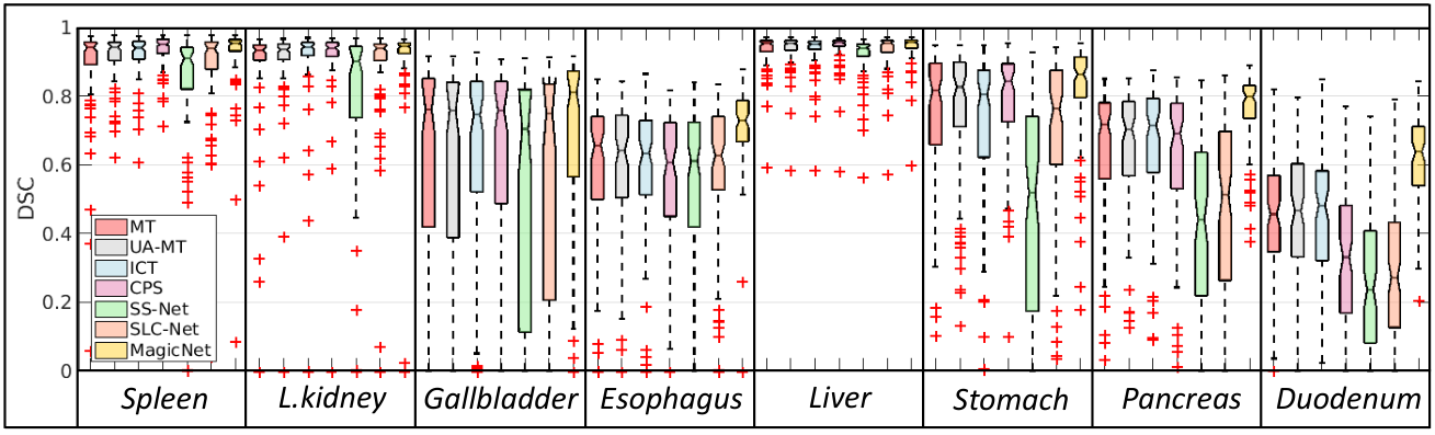
We then evaluate MagicNet on MACT dataset. In Table 2, we can observe: (1) a more significant performance improvement between MagicNet and other state-of-the-arts with 10% labeled data than 20%, which demonstrates the effectiveness of MagicNet when training with fewer labeled CT images; (2) MagicNet successfully mitigates the inferior performance in tail classes, e.g., DSC improvement with 10% labeled images on Gallbladder ($\uparrow$ 4.88), Esophagus ($\uparrow$ 11.52), Pancreas ($\uparrow$ 10.45) and Duodenum ($\uparrow$ 16.50). Fig. 5 shows a comparison in DSC of six methods for different organs. Note that UMCT Xia2020uncertainty on MACT dataset achieves 75.33% in DSC. It uses AH-Net liu20183d as the backbone (3 are used), whose parameter number is much larger. Due to computation resources, we do not directly compare with it.

We conduct ablation studies on MACT datasetdensevnet2018TMI with 10% labeled data to show the effectiveness of each module.

References

- (1) Wenjia Bai, Ozan Oktay, Matthew Sinclair, Hideaki Suzuki, Martin Rajchl, Giacomo Tarroni, Ben Glocker, Andrew P. King, Paul M. Matthews, and Daniel Rueckert. Semi-supervised learning for network-based cardiac MR image segmentation. In Proc. MICCAI, 2017.
- (2) David Berthelot, Nicholas Carlini, Ekin D. Cubuk, Alex Kurakin, Kihyuk Sohn, Han Zhang, and Colin Raffel. Remixmatch: Semi-supervised learning with distribution matching and augmentation anchoring. In Proc. ICLR, 2020.
- (3) David Berthelot, Nicholas Carlini, Ian J. Goodfellow, Nicolas Papernot, Avital Oliver, and Colin Raffel. Mixmatch: A holistic approach to semi-supervised learning. In Proc. NeurIPS, 2019.
- (4) Gerda Bortsova, Florian Dubost, Laurens Hogeweg, Ioannis Katramados, and Marleen de Bruijne. Semi-supervised medical image segmentation via learning consistency under transformations. In Proc. MICCAI, 2019.
- (5) Hu Cao, Yueyue Wang, Joy Chen, Dongsheng Jiang, Xiaopeng Zhang, Qi Tian, and Manning Wang. Swin-unet: Unet-like pure transformer for medical image segmentation. arXiv preprint arXiv:2105.05537, 2021.
- (6) Jieneng Chen, Yongyi Lu, Qihang Yu, Xiangde Luo, Ehsan Adeli, Yan Wang, Le Lu, Alan L Yuille, and Yuyin Zhou. Transunet: Transformers make strong encoders for medical image segmentation. arXiv preprint arXiv:2102.04306, 2021.
- (7) Xiaokang Chen, Yuhui Yuan, Gang Zeng, and Jingdong Wang. Semi-supervised semantic segmentation with cross pseudo supervision. In Proc. CVPR, 2021.
- (8) Terrance DeVries and Graham W Taylor. Improved regularization of convolutional neural networks with cutout. arXiv preprint arXiv:1708.04552, 2017.
- (9) Kang Fang and Wu-Jun Li. Dmnet: Difference minimization network for semi-supervised segmentation in medical images. In Proc. MICCAI, 2020.
- (10) Shuhao Fu, Yongyi Lu, Yan Wang, Yuyin Zhou, Wei Shen, Elliot Fishman, and Alan Yuille. Domain adaptive relational reasoning for 3d multi-organ segmentation. In Proc. MICCAI, 2020.
- (11) Eli Gibson, Francesco Giganti, Yipeng Hu, Ester Bonmati, Steve Bandula, Kurinchi Gurusamy, Brian Davidson, Stephen P. Pereira, Matthew J. Clarkson, and Dean C. Barratt. Automatic multi-organ segmentation on abdominal ct with dense v-networks. IEEE Trans. Medical Imaging, 37(8):1822–1834, 2018.
- (12) Yuanfeng Ji, Haotian Bai, Jie Yang, Chongjian Ge, Ye Zhu, Ruimao Zhang, Zhen Li, Lingyan Zhang, Wanling Ma, Xiang Wan, et al. Amos: A large-scale abdominal multi-organ benchmark for versatile medical image segmentation. arXiv preprint arXiv:2206.08023, 2022.
- (13) Bennett Landman, Zhoubing Xu, J Igelsias, Martin Styner, T Langerak, and Arno Klein. Miccai multi-atlas labeling beyond the cranial vault–workshop and challenge. In Proc. MICCAI Workshop, 2015.
- (14) Shuailin Li, Chuyu Zhang, and Xuming He. Shape-aware semi-supervised 3d semantic segmentation for medical images. In Proc. MICCAI, 2020.
- (15) Xiaomeng Li, Lequan Yu, Hao Chen, Chi-Wing Fu, and Pheng-Ann Heng. Transformation consistent self-ensembling model for semi-supervised medical image segmentation. IEEE Trans. Neural Networks and Learning Systems, 32(2):523–534, 2020.
- (16) Jinhua Liu, Christian Desrosiers, and Yuanfeng Zhou. Semi-supervised medical image segmentation using cross-model pseudo-supervision with shape awareness and local context constraints. In Proc. MICCAI, 2022.
- (17) Siqi Liu, Daguang Xu, S Kevin Zhou, Olivier Pauly, Sasa Grbic, Thomas Mertelmeier, Julia Wicklein, Anna Jerebko, Weidong Cai, and Dorin Comaniciu. 3d anisotropic hybrid network: Transferring convolutional features from 2d images to 3d anisotropic volumes. In Proc. MICCAI, 2018.
- (18) Xiangde Luo, Jieneng Chen, Tao Song, and Guotai Wang. Semi-supervised medical image segmentation through dual-task consistency. In Proc. AAAI, 2021.
- (19) Jun Ma, Yao Zhang, Song Gu, Cheng Zhu, Cheng Ge, Yichi Zhang, Xingle An, Congcong Wang, Qiyuan Wang, Xin Liu, Shucheng Cao, Qi Zhang, Shangqing Liu, Yunpeng Wang, Yuhui Li, Jian He, and Xiaoping Yang. Abdomenct-1k: Is abdominal organ segmentation a solved problem? IEEE Trans. Pattern Anal. Mach. Intell., 44(10):6695–6714, 2022.
- (20) Fausto Milletari, Nassir Navab, and Seyed-Ahmad Ahmadi. V-net: Fully convolutional neural networks for volumetric medical image segmentation. In Proc. 3DV, 2016.
- (21) Holger R Roth, Le Lu, Amal Farag, Hoo-Chang Shin, Jiamin Liu, Evrim B Turkbey, and Ronald M Summers. Deeporgan: Multi-level deep convolutional networks for automated pancreas segmentation. In Proc. MICCAI, 2015.
- (22) Holger R. Roth, Hirohisa Oda, Xiangrong Zhou, Natsuki Shimizu, Ying Yang, Yuichiro Hayashi, Masahiro Oda, Michitaka Fujiwara, Kazunari Misawa, and Kensaku Mori. An application of cascaded 3d fully convolutional networks for medical image segmentation. Comput. Medical Imaging Graph., 66:90–99, 2018.
- (23) Yinghuan Shi, Jian Zhang, Tong Ling, Jiwen Lu, Yefeng Zheng, Qian Yu, Lei Qi, and Yang Gao. Inconsistency-aware uncertainty estimation for semi-supervised medical image segmentation. IEEE Trans. Medical Imaging, 41(3):608–620, 2022.
- (24) Kihyuk Sohn, David Berthelot, Nicholas Carlini, Zizhao Zhang, Han Zhang, Colin Raffel, Ekin Dogus Cubuk, Alexey Kurakin, and Chun-Liang Li. Fixmatch: Simplifying semi-supervised learning with consistency and confidence. In Proc. NeurIPS, 2020.
- (25) Hao Tang, Xuming Chen, Yang Liu, Zhipeng Lu, Junhua You, Mingzhou Yang, Shengyu Yao, Guoqi Zhao, Yi Xu, Tingfeng Chen, Yong Liu, and Xiaohui Xie. Clinically applicable deep learning framework for organs at risk delineation in CT images. Nat. Mach. Intell., 1(10):480–491, 2019.
- (26) Yucheng Tang, Riqiang Gao, Ho Hin Lee, Shizhong Han, Yunqiang Chen, Dashan Gao, Vishwesh Nath, Camilo Bermudez, Michael R. Savona, Richard G. Abramson, Shunxing Bao, Ilwoo Lyu, Yuankai Huo, and Bennett A. Landman. High-resolution 3d abdominal segmentation with random patch network fusion. Medical Image Anal., 69:101894, 2021.
- (27) Yucheng Tang, Dong Yang, Wenqi Li, Holger R Roth, Bennett Landman, Daguang Xu, Vishwesh Nath, and Ali Hatamizadeh. Self-supervised pre-training of swin transformers for 3d medical image analysis. In Proc. CVPR, 2022.
- (28) Antti Tarvainen and Harri Valpola. Mean teachers are better role models: Weight-averaged consistency targets improve semi-supervised deep learning results. In Proc. NeurIPS, 2017.
- (29) Peng Tu, Yawen Huang, Feng Zheng, Zhenyu He, Liujuan Cao, and Ling Shao. Guidedmix-net: Semi-supervised semantic segmentation by using labeled images as reference. In Proc. AAAI, 2022.
- (30) Vikas Verma, Alex Lamb, Juho Kannala, Yoshua Bengio, and David Lopez-Paz. Interpolation consistency training for semi-supervised learning. In Proc. IJCAI, 2019.
- (31) Kaiping Wang, Bo Zhan, Chen Zu, Xi Wu, Jiliu Zhou, Luping Zhou, and Yan Wang. Semi-supervised medical image segmentation via a tripled-uncertainty guided mean teacher model with contrastive learning. Medical Image Anal., 79:102447, 2022.
- (32) Qin Wang, Wen Li, and Luc Van Gool. Semi-supervised learning by augmented distribution alignment. In Proc. ICCV, 2019.
- (33) Yan Wang, Yuyin Zhou, Wei Shen, Seyoun Park, Elliot K. Fishman, and Alan L. Yuille. Abdominal multi-organ segmentation with organ-attention networks and statistical fusion. Medical Image Anal., 55:88–102, 2019.
- (34) Chen Wei, Lingxi Xie, Xutong Ren, Yingda Xia, Chi Su, Jiaying Liu, Qi Tian, and Alan L. Yuille. Iterative reorganization with weak spatial constraints: Solving arbitrary jigsaw puzzles for unsupervised representation learning. In Proc. CVPR, 2019.
- (35) Yicheng Wu, Zhonghua Wu, Qianyi Wu, Zongyuan Ge, and Jianfei Cai. Exploring smoothness and class-separation for semi-supervised medical image segmentation. In Proc. MICCAI, 2022.
- (36) Yingda Xia, Dong Yang, Zhiding Yu, Fengze Liu, Jinzheng Cai, Lequan Yu, Zhuotun Zhu, Daguang Xu, Alan L. Yuille, and Holger Roth. Uncertainty-aware multi-view co-training for semi-supervised medical image segmentation and domain adaptation. Medical Image Anal., 65:101766, 2020.
- (37) Lingxi Xie, Qihang Yu, Yuyin Zhou, Yan Wang, Elliot K. Fishman, and Alan L. Yuille. Recurrent saliency transformation network for tiny target segmentation in abdominal ct scans. IEEE Trans. Medical Imaging, 39(2):514–525, 2020.
- (38) Chenyu You, Yuan Zhou, Ruihan Zhao, Lawrence H. Staib, and James S. Duncan. Simcvd: Simple contrastive voxel-wise representation distillation for semi-supervised medical image segmentation. IEEE Trans. Medical Imaging, 41(9):2228–2237, 2022.
- (39) Lequan Yu, Shujun Wang, Xiaomeng Li, Chi-Wing Fu, and Pheng-Ann Heng. Uncertainty-aware self-ensembling model for semi-supervised 3d left atrium segmentation. In Proc. MICCAI, 2019.
- (40) Sangdoo Yun, Dongyoon Han, Seong Joon Oh, Sanghyuk Chun, Junsuk Choe, and Youngjoon Yoo. Cutmix: Regularization strategy to train strong classifiers with localizable features. In Proc. ICCV, 2019.
- (41) Hongyi Zhang, Moustapha Cissé, Yann N. Dauphin, and David Lopez-Paz. mixup: Beyond empirical risk minimization. In Proc. ICLR, 2018.
- (42) Xinkai Zhao, Chaowei Fang, De-Jun Fan, Xutao Lin, Feng Gao, and Guanbin Li. Cross-level contrastive learning and consistency constraint for semi-supervised medical image segmentation. In Proc. ISBI, 2022.
- (43) Yuyin Zhou, Yan Wang, Peng Tang, Song Bai, Wei Shen, Elliot K. Fishman, and Alan L. Yuille. Semi-supervised 3d abdominal multi-organ segmentation via deep multi-planar co-training. In Proc. WACV, 2019.