Generating entangled states from coherent states in circuit-QED
Abstract
Entangled states are self-evidently important to a wide range of applications in quantum communication and quantum information processing. We propose an efficient and convenient two-step protocol for generating Bell states and NOON states of two microwave resonators from merely coherent states. In particular, we derive an effective Hamiltonian for resonators coupled to a superconducting -type qutrit in the dispersive regime. By the excitation-number-dependent Stark shifts of the qutrit transition frequencies, we are able to individually control the amplitudes of specified Fock states of the resonators associated with relevant qutrit transition, using carefully tailored microwave drive signals. Thereby an arbitrary bipartite entangled state in Fock space can be generated by a typical evolution-and-measurement procedure. We analysis the undesired state transitions and the robustness of our protocol against the systematic errors from the microwave driving intensity and frequency, the quantum decoherence of all components, and the crosstalk of two resonators. In addition, we demonstrate that our protocol can be extended to a similar scenario with a -type qutrit.
I Introduction
Entangled states Horodecki et al. 2009 of harmonic oscillators, e.g., microwave resonators, play a key role in quantum technologies, such as quantum communication Gisin and Thew 2007 and quantum information processing Bennett and DiVincenzo 2000. Creation, manipulation, and measuring of the entangled states in both experimental platforms Mølmer and Sørensen 1999; Wei et al. 2006; Yang et al. 2016; Erhard et al. 2018; Song et al. 2019 and theoretical protocols have therefore been intensively pursued for a long time Bouwmeester et al. 1999; Wei et al. 2006; Bishop et al. 2009; Macrì et al. 2018; Paul and Sarma 2016; Strauch et al. 2010; Merkel and Wilhelm 2010; Lee and Kim 2000 and are still under an active investigation.
The simplest and yet the most popular maximally entangled states in the Fock space of the resonators are Bell states, i.e., and , where and are the ground and the first excited states, respectively. Generating Bell states in photonic systems is fundamental to both quantum cryptography Tittel et al. 2000 and quantum teleportation Kim et al. 2001. Another widely applied entangled states are the NOON states with integer, consisting of two orthogonal components in an equal-weighted superposition Dowling 2008; D’Angelo et al. 2008; Kamide et al. 2017; Chen and Wei 2017; Wang et al. 2016. They are crucial elements in quantum metrology Mitchell et al. 2004; Pezzè et al. 2018, quantum optical lithography Boto et al. 2000; D’Angelo et al. 2001, and quantum information processing Bennett and DiVincenzo 2000. The NOON states have been realized in multiple quantum systems, including polarization states of photons Israel et al. 2014, nuclear spin of molecules Jones et al. 2009, optical paths of photons Afek et al. 2010, ultracold dipolar atoms in optical superlattice setup Grün et al. 2022a; Grün et al. 2022b, and phonons in ion trap Zhang et al. 2018. Nevertheless, the multi-step ultra-precise control over the quantum devices, the specialization of the initial states, and the decoherence of quantum systems make it hard to create and hold highly-entangled states. Fast and convenient protocols for preparing either Bell state or NOON state are still underway.
With unique properties including long coherent time Yan et al. 2015; You et al. 2007; Peterer et al. 2015 and strong and even ultrastrong dipole-dipole coupling Wallraff et al. 2004; Peropadre et al. 2010; Forn-Díaz et al. 2019; Kockum et al. 2019; Niemczyk et al. 2010, the circuit-QED system You and Franco 2011; Blais et al. 2021 has been used as a promising platform to generate nonclassical states and entangled states Zhao et al. 2015; Wei et al. 2006; Wallraff et al. 2004; Peropadre et al. 2010. Many protocols have thus been proposed upon the manipulation capability up to the artificial atomic level. It is noted that most of the existing generation protocols Macrì et al. 2018; Paul and Sarma 2016; Strauch et al. 2010; Merkel and Wilhelm 2010; Wang et al. 2011; Su et al. 2014; Xiong et al. 2015; Su et al. 2017; Qi and Jing 2020 are developed on Rabi oscillations and initialization of the resonator. For example, by tuning the atomic frequency to be resonant with the resonator, the excitation of the artificial atom is transferred to the resonator mode through a half of Rabi oscillation. The NOON state with a significant number is then generated by a step-by-step processing with resonators prepared as the ground state, that is fragile to both systematic error and environmental noise.

In this work, we propose a two-step protocol for entangling two resonators that are dispersively coupled to a superconducting qutrit Wallraff et al. 2004; Peropadre et al. 2010; You and Franco 2011. As shown in Fig. 1, the flux-driven qutrit You and Franco 2011 presents various configuration by the magnitude of the magnetic flux. At a particular point with , it behaves as a -type qutrit. When , the parity symmetry is broken; all three dipole transitions among , , and are allowed; and the qutrit becomes a -type one. The resonators are initially in separable coherent states, which can be conveniently created by classical drives Wang et al. 2017. The main ingredients of our protocol are the excitation-number-dependent qutrit rotations, allowing individually manipulating the probability amplitudes of the Fock-state components of coherent states by carefully tailoring the microwave drive signals. The excitation-number-dependent Stark shift in the qutrit transition frequency arises from the qutrit-resonator interaction Guo et al. 2008; Zueco et al. 2009. It has been used to realize dressed coherent states Govia and Wilhelm 2016, entangled states in discrete or discrete-continuous systems Gerry 1996; Su et al. 2021, quantum phase gate Zou et al. 2007; Zhang et al. 2017, and hybrid Fredkin gate Liu et al. 2018. Experimentally it was reported to generate arbitrary Fock states Wang et al. 2017 in circuit-QED system.
In Sec. II, we introduce our model of two resonators coupled to a -type qutrit and derive the effective Hamiltonian at the dispersive regime. In Sec. III, we provide a detailed protocol for generating a bipartite entangled state in Fock space. Appendix A, we discuss the nonideal measurement. We analysis in Sec. IV.1 the final state fidelity in the presence of unsuppressed state-transitions. The detailed calculation is provided in Appendix B. The systematic errors from the driving intensity and frequency, the decoherence noises for the overall qutrit-resonator system, and the unwanted couplings in the whole system are respectively addressed in Sec. IV.2, Sec. IV.3, and Sec. IV.4. In Sec. V, our protocol is extended to the -type transmon qutrit. The whole work is summarized in Sec. VI.
II Model and the effective Hamiltonian
Consider a -type qutrit as shown in Fig. 1(c) coupled to two microwave resonators Blais et al. 2021 (labeled and ). The three levels of the qutrit , , and denote respectively the ground state, the intermediate state, and the highest-level state. The system Hamiltonian () is given by
| (1) | ||||
where () is the transition frequency of the resonator (), () represents the free level spacing between the state () and the ground state.
With proper parameters in junctions, the elements in the transition matrix describing and are dominant over that for in magnitude, i.e., You and Franco 2011. The -type qutrit could thus be simplified as the -type. Through frequency manipulation, the resonator () can only be significantly coupled to the () transition. The two transitions are assumed to be sufficiently detuned or decoupled from each other and then these two couplings contribute to independent Rabi transitions. Thus, the interaction Hamiltonian in Eq. (1) can be approximated as
| (2) | ||||
where and .
In the dispersive regime, i.e., and , can be considered as a perturbation with respect to the free Hamiltonian . Across the whole Hilbert space, the interaction Hamiltonian would give rise to the energy shift of any eigenstate of the unperturbed Hamiltonian in Eq. (1). To the second order, the energy shift is effectively given by
| (3) |
where and is the eigenenergy of . For , the eigenstates read , , and .
Summarizing the two paths starting from and going back to through an intermediate state, i.e., and , one can obtain the second-order correction in energy for the state ,
| (4) |
according to Eq. (3). In the same way, one can obtain the corrected energy for the state
| (5) |
and the corrected energy for the state
| (6) |
where
| (7) | ||||
are the energy shifts due to the interaction Hamiltonian , describing the virtual two-photon processes in Eq. (3). Note ’s and ’s are contributions from rotating-wave interaction and counterrotating terms, respectively. The presence or absence of the counterrotating terms does not violate the following derivation and protocol.
It is noted that and are arbitrarily Fock states in the preceding analysis. Thus, in the dispersive regime, the effective Hamiltonian can be written as
| (8) | ||||
where the last two lines describe the excitation-number-dependent Stark shifts for all the three atomic levels.
III Two-step generation protocol

In this section, we show how to generate a bipartite entangled state of two resonators in the form of , and , from coherent states by the effective Hamiltonian in Eq. (8). The whole protocol is visually summarized in Fig. 2.
Suppose that the qutrit is initially in the superposed state and the two resonators and are prepared in the coherent states and , respectively. The whole system starts from
| (9) | ||||
where and are complex numbers. Alternatively, the initial state can be written as
| (10) |
where is the normalization coefficient. The initial coherent state can be achieved by the application of a microwave pulse on the resonator, that produces a displacement operation on the vacuum state and Wang et al. 2017.
Step-: Applying two microwave pulses and that are nearly resonant with the qutrit transitions and , respectively. Here is the intensity of the driving pulses satisfying with the duration time and , , is the driving frequency. The total Hamiltonian including the driving pulses can then be written as
| (11) | ||||
In the rotating frame with respect to , it turns out to be
| (12) | ||||
Consequently, if one chooses
| (13) | ||||
then in the Fock space, the total Hamiltonian could be rewritten as
| (14) | ||||
where the nonvanishing detunings read
| (15) | ||||
In the ideal weak-driving regime, these detunings and are much larger than the Rabi frequency, i.e., . In this case, the first driving pulse resonantly drives the qutrit transition and the number state of the resonator modes and its impact on the other number states could be averaged out in a properly long time-scale . Similarly, the second driving pulse resonantly drives the state transition and also does not significantly affect the number states other than . Driven by the total Hamiltonian in Eq. (14) with secular approximation, the initial state of the system evolves as
| (16) | ||||
After a period of , we have
| (17) | ||||
The two tailored microwave pulses could be separably applied to the system. One can first drive the transition by the microwave pulse . The total Hamiltonian under the secular approximation is thus described by H.c.. Then after a period , the state evolves into without invoking the other transitions. Next another microwave pulse is applied to transfer to . The state in Eq. (17) is eventually achieved.
Step-: Performing the measurement on the qutrit by the projection operator Caves et al. 1980; Bocko and Onofrio 1996. Consequently, the reduced density operator of two resonator modes becomes
| (18) |
where the denominator is the success probability Yan and Jing 2022a; Yan and Jing 2022b and means partial trace over the qutrit. Up to a dynamical phase accumulated in evolution, is an entangled state fully determined by and specified in Eq. (13),
| (19) |
where
| (20) |
A balanced superposition requires that . Hereafter both and are supposed to be positive numbers for simplicity. Up to a local phase, we have generated an arbitrary entangled state for two continuous-variable modes with a success probability
| (21) |
Here are two distinguishing instances. With and , one can obtain a double-excitation Bell state
| (22) |
by setting the coherent-state parameters as . With , , and , the entangled state in Eq. (19) turns out to be a NOON state
| (23) |
The efficiency of our protocol for generating can be quantified by the state fidelity
| (24) |
where is the density matrix directly obtained by Eq. (14) without secular approximation. We also ignore the dynamical phase of the time-evolved state in practical numerical simulation. The protocol depends on a perfect performance by measurement operator . The influence from a nonideal measurement on the state fidelity is shown in Appendix A. We stick to the ideal measurement in the following analysis about fidelity.
IV Fidelity analysis
IV.1 Undesired transition in the presence of driving
The state evolution under the secular approximation in Step- of Sec. III reflects the ideal assumption that the microwave driving pulses can only affect the desired pairs of states and filtered out by choosing the driving frequency in Eq. (13). The two driving pulses might however induce the other state transitions that invalidate the secular-approximation condition . Given the initial state in Eq. (10), the fidelity of the entangled state in Eq. (19) is found to be
| (25) |
under both desired and undesired transitions. Here , and . is obtained by replacing with . Note . The detunings and are given by Eq. (15). The derivation details can be found in Appendix B.
This result is consistent with the condition that both and should be sufficiently larger than . Then the undesired transitions are ignorable and does not obstruct generating the desired entangled state with a high fidelity. However, this condition cannot be always satisfied for arbitrary . Similar to Eqs. (13) and (15), certain detunings and approach vanishing when the Fock states indicated by and follow the same equations as the desired pairs of and :
| (26) | ||||
If the coupling strength between qutrit and resonator is sufficiently weak, e.g., , then the energy shifts induced by the counterrotating interactions H.c. and H.c. would be much less than the energy shifts induced by the rotating-wave interactions H.c. and H.c. as implied by Eq. (7). It is then interesting to find that Eq. (26) can be met under the conditions
| (27) | ||||
where , , , and are nonnegative integers representing the shifts from the desired Fock states and . In other words, the states () would evolve to () in parallel to the desired transition () with a nonnegligible probability under the same driving in Eq. (11).
To reduce the probability of the undesired state transitions, one can properly choose and so that the populations on the states and become significantly less than those on and . This requirement is satisfied when the “state-shift” ratios and are irreducible ratios of integers larger than the average number of excitations for the fixed initial coherent states, i.e., or . Due to Eq. (27), the “state-shift” ratios are twice the energy-shift ratios. And according to Eq. (7), is determined by the transition frequencies of the qutrit and two resonators,
| (28) |
when the coupling strengths are isotropic . The ratio is thus an important element to the state fidelity, which can be properly adjusted by the frequencies of the system components. Its value should not be taken in the proximity of an irreducible ratio of small integers.

Figure 3 confirms our two-step protocol in generating the NOON state from coherent states with . The state fidelity obtained by Eq. (24) or Eq. (25) is plotted under various Rabi frequencies of the driving pulses in the total Hamiltonian (14). For arbitrary , would become invalid with a higher probability under a larger . For example, the fidelity of the NOON state with is when and it declines to when the Rabi frequency is enhanced to . On the other hand, one can find that a larger gives rise to a smaller fidelity and the decline magnitude increases by increasing . In comparison to the state of , the state fidelity for declines from () to ().

To avoid the participation of the undesired state transition involving and , the ratio of in Fig. 3 is set to be . Both numerator and denominator are sufficiently distinct from either or . In Fig. 4, we plot the NOON state fidelity as a function of in the range of . As expected, the fidelity declines when increasing the Fock number . More importantly, one can observe that the fidelity declines significantly at certain values that could be expressed by irreducible ratio of small integers, e.g., , , and . It can be theoretically explained by Eq. (27). For example, gives rise to . Under this condition, in parallel to the desired state transition , we have an undesired evolution described by under the total Hamiltonian (14). Similarly, the populations on the states and cannot be ignored if the target transition is . In contrast, the fidelities are nearly unit at the other points, e.g., and , where the population on satisfying the condition in Eq. (27) is significant less than that on the target state , regarding . Thus, a high-fidelity entangled state can be achieved by properly choosing the initial coherent states of the resonators and the level spacings in ancillary qutrit.
IV.2 Systematic errors on driving pulses
From Eqs. (16) and (17), it is important for our protocol to perform the measurement at the keypoint . Then it seems that the driving intensities for both and have to take the same magnitude. And the driving frequencies and should be exactly determined by Eq. (13) to realize the desired state evolution. The control might not be exactly implemented because of the technical imperfections and constrains. In this subsection, we consider the systematic errors raised by the unequal driving intensities and the deviations in driving frequencies.
We first consider that the two driving intensities depart from each other by a relative magnitude . In particular, the driving Hamiltonian in Eq. (11) is rewritten as
| (29) |
and consequently the total Hamiltonian (14) in rotating frame becomes
| (30) | ||||
With the Hamiltonian in Eq. (30), the initial state in Eq. (10) evolves to
| (31) | ||||
when . Then we measure the qutrit with the projection operator , one can still obtain the (unnormalized) target state
| (32) |
Since is a common factor, the error on driving intensity can therefore be ignored in the ideal situation that the microwave pulses only drive the desired states. Its effect, however, emerges when considering the undesired evolution induced by vanishing and as discussed in Sec. IV.1.


Under the Hamiltonian (30) with the intensity error, the fidelities of the double-excitation Bell state and the NOON state are presented in Fig. 5 and Fig. 6, respectively, as a function of . The fidelities are evaluated at the desired moment as requested by Step- in our protocol.
It is found in Fig. 5 that the fidelity sensitivity to the intensity error is amplified with increasing Rabi frequency . In particular, for , the fidelities are roughly invariant in the presence of , even when it is about . And for , it declines slightly with when it increases from to . This result could be understood since the condition becomes less reliable for a larger . In Fig. 6, the results for various are obtained under . Although a larger gives rise to more decay, the fidelities can still be maintained over with about errors in the driving intensity. Thus, one can conclude that our protocol is robust against the fluctuations on the Rabi frequencies. We can have a high fidelity as long as the measurement moment is determined by the average of these Rabi frequencies.
As for the deviation in driving frequency, we have
| (33) |
Here the relative errors for the two driving frequencies are assumed to take the same magnitude with and then the total Hamiltonian in the rotating frame with respect to is rewritten as
| (34) | ||||
Consequently, the initial state evolves to
| (35) | ||||
at the desired time , where
| (36) | ||||
with and . Then one can obtain
| (37) |
by performing the projective measurement . Up to the second order of , it is found that
| (38) |
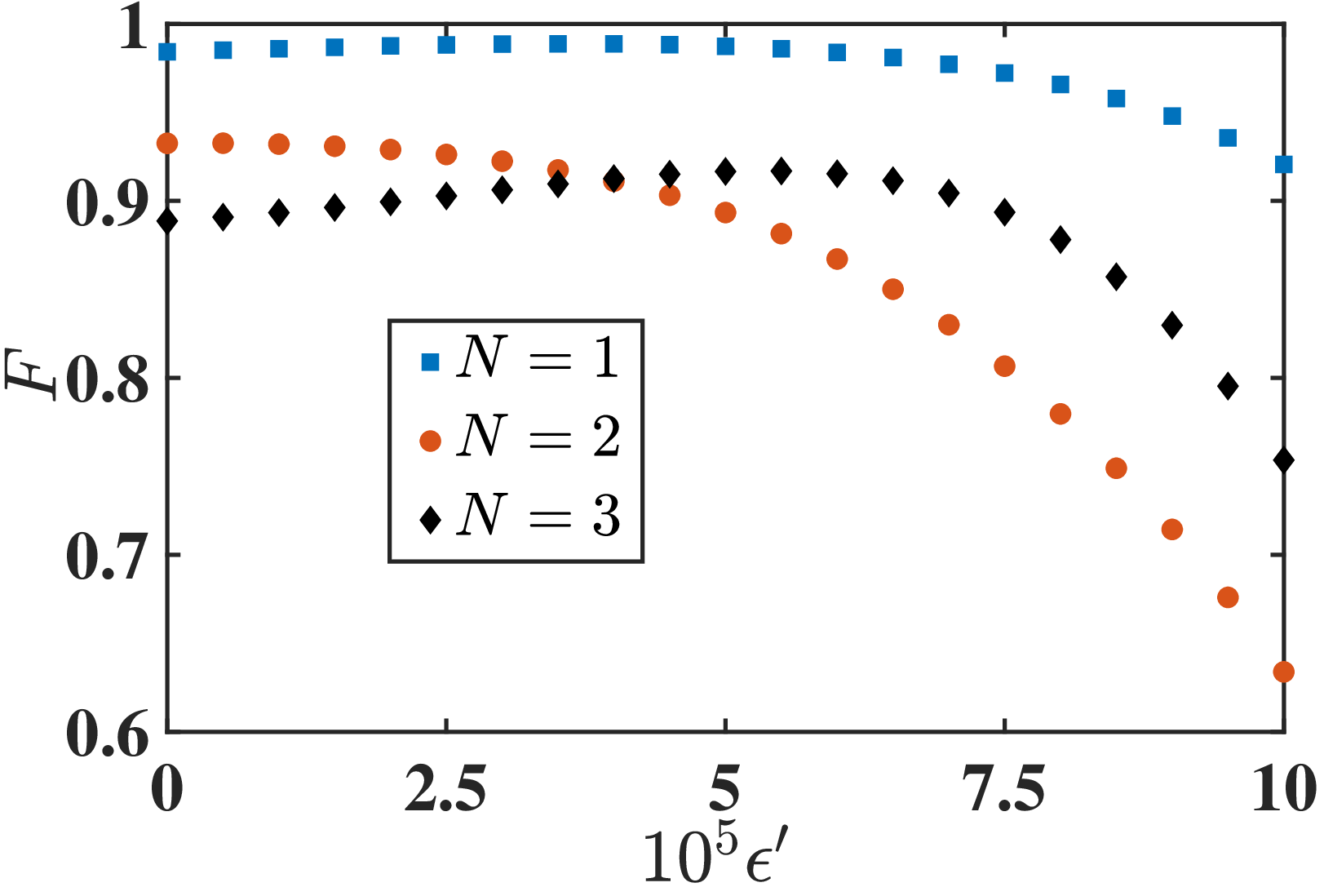
The fidelity sensitivity for the NOON state to the frequency error is demonstrated in Fig. 7. For , the fidelity declines slightly with and it can be maintained over when the error magnitude approaches . The decline rate becomes larger for and the fidelity is about when . The behavior of fidelity for is not monotonic. It first increases until and then gradually decreases to when . In comparison to Fig. 6, our protocol is therefore less robust against the error in the driving frequency than that in the driving intensity.
IV.3 External decoherence
During the state generation, the composite system can not be completely isolated from the surrounding environment. The target entangled state will be damaged by the influence from both resonator damping and qutrit decoherence. Taking the local decoherence channels into consideration, we can study the entangled state generation fidelity in a standard open-quantum-system framework. Under the Markovian approximation and tracing out the degrees of freedom of the external environments (assumed to be at the vacuum states), we arrive at the master equation for the density operator for the composite system
| (39) | ||||
Here is the total Hamiltonian in Eq. (14). and are the population relaxation constants associated with the transitions and , respectively. and are the dephasing rates associated with the states and , respectively. For simplicity, these decoherence rates of qutrit are assumed to take the same value . () is the decay constant of the resonator mode (). We set for the resonator lifetime is higher than the qutrit lifetime in realistic experimental platforms Yurtalan et al. 2021; Reagor et al. 2016; Blais et al. 2021. The Lindblad superoperator is defined as
| (40) |

The fidelity of the target state under various Rabi frequencies and decoherence rates is shown in Fig. 8. In the presence of a larger decoherence rate (the left region in the figure), a smaller Rabi frequency cannot yield a higher fidelity as in Figs. (3) and (5). We have to make a compromise of to optimize the fidelity since the desired period of the state generation is inversely proportional to the and the decoherence becomes more severe under a longer evolution time. It is found that the fidelity in two optimized regimes is maintained above . One is around even when is nearly ; another one is around when .

In Fig. 9, we present the impact of decoherence on the NOON state fidelity under . The fidelity declines with the increasing Fock number and it is not sensitive to the decoherence rate when . For , the fidelities are , , , , and for , respectively. A significant decline in fidelity occurs under a stronger decoherence rate . It is about for .
For such a system of a flux qutrit and two resonators Yan et al. 2015; Peterer et al. 2015; Wallraff et al. 2004; You and Franco 2011, the transition frequencies among the lowest three levels of the qutrit can be manipulated within the range of GHz, and the frequencies of the resonators are in the order of GHz. The coupling between qutrit and resonators has entered the strong and even ultrastrong coupling regimes Wallraff et al. 2004; Peropadre et al. 2010, i.e., . The coherence timescale of the qutrit is about Yurtalan et al. 2021, corresponding to . The quality factor of the resonators is about Blais et al. 2021, and even approaches Reagor et al. 2016, corresponding to . Then we set and in preceding calculations.
IV.4 Unwanted couplings
In addition to the external noises, our protocol could be also subject to the unwanted couplings inside the system. In Sec. II, we use a -type qutrit to approximate the realistic -type qutrit, depending on the suppressed dipole-dipole transition between and . This transition is however unavoidable under [see Fig. 1(c)]. In this case, the interaction Hamiltonian in the initial Hamiltonian (1) is then rewritten as
| (41) | ||||
To simplify the discussion but with no loss of generality, it is assumed that , . With the second-order perturbation method presented in Eq. (3), the effective Hamiltonian in Eq. (8) for the whole system is modified to
| (42) | ||||
where the energy shifts read
| (43) |
We here employ the step function , i.e., when and when .
The driving Hamiltonian in Eq. (11) is still applicable to distinguish the desired state transitions and . Under the modified effective Hamiltonian in Eq. (42), it is found that the two frequencies of microwave pulses in Eq. (13) are respectively modified to
| (44) | ||||
The total Hamiltonian in analog to Eq. (11) is then written as
| (45) |
Subsequently one can carry out a similar rotation as in Step- in our protocol to obtain the desired time-independent Hamiltonian in Eq. (14). Under the secular approximation, it is used to push the system into the state in Eq. (17) for Step-.
It is straightforward to check that the transition frequencies and in Eq. (13) could be respectively recovered by and when the energy shifts and . It is consistent with the fact that the -type qutrit could be approximated by the -type qutrit in Sec. II. In this case, , , , and , where , , , and have been given in Eq. (7).

In Fig. 10, we present the NOON state fidelity by using the Lindblad master equation (39) with for the -type qutrit and for the -type one. The extra decoherence channel described by has been taken account into Eq. (39) with the same dissipation rate when we consider the -type qutrit. We find that the discrepancy between the -type and the -type is enlarged by the decoherence rate. For example, for , the fidelity of the -type qutrit is under , which is almost the same as that of the -type . In contrast, the fidelity under declines to and for the -type and the -type, respectively. Note the decoherence rates in practice satisfy You and Franco 2011. Our calculation about the -type qutrit could thus be regarded as a lowerbound estimation.

Another unwanted coupling arises from the crosstalk between the two resonators and . In this situation, the interaction Hamiltonian in Eq. (2) becomes
| (46) |
where is the inter-resonator coupling strength. Then the total Hamiltonian in Eq. (11) turns out to be
| (47) |
In Fig. 11, the NOON state fidelities under various crosstalk coupling strength are calculated in the absence of decoherence. The crosstalk is also found to be a negative ingredient to the fidelity of the generated state for any . Yet its effect is not significant. For , comparing to when , the fidelity can be maintained as even when .
V Discussion
In addition to the -type qutrit for as discussed in Sec IV.4, our protocol can be implemented by a -type transmon qutrit with a specific ratio [see Fig. 1(b)]. In this case, the total Hamiltonian in Eq. (1) could be rewritten as
| (48) | ||||
In the absence of the crosstalk between the two resonators, the effective Hamiltonian under the second-order perturbation (3) becomes
| (49) | ||||
where
| (50) | ||||
Similar to Eq. (8), this effective Hamiltonian again describes the photon-number-dependent Stark shifts for each energy levels of qutrit. Following the same procedure illustrated in Sec. III, we can create an entangled state from the initial state by using tailored pulses transferring the states and and then measuring the qutrit with the projection operator . Also we can apply the Lindblad master equation (39) to estimate the entangled-state fidelities using a -type qutrit under decoherence, where the dissipation channel is now replaced by .
| 1 | 2 | 3 | 4 | 5 | |
|---|---|---|---|---|---|
| 0.964 | 0.924 | 0.880 | 0.781 | 0.714 | |
| 0.917 | 0.891 | 0.736 | 0.412 | 0.124 |
In Table. 1, we find that all fidelities with the -type qutrit are smaller than those with the -type one, although the decoherence rate of the former is half of the latter. And their difference is enlarged by . In our main protocol with the -type qutrit, where the initial state is a superposed state of the two lowest levels and . No extra decoherence channel populates the highest level that serves as the measured state. While in the protocol with the -type qutrit, the initial state is a superposed state of and . The measured middle level is under a severe influence from the population relaxation by . The final state fidelity with the -type qutrit is therefore not as high as that with the -type one.
VI Conclusion
In summary, we have presented a concise two-step protocol for creating an arbitrary bipartite entangled state in Fock space of two microwave resonators that are strongly coupled to a superconducting qutrit. No extra steps have to be taken to shape the initial states of the resonators. With a second-order perturbation method, the system could be described by an effective Hamiltonian in the dispersive regime. We take advantage of the excitation-number-dependent Stark shift for the qutrit transition frequency. It allows us to apply tailored microwave drive signals to individually control the qutrit transition amplitudes associated with the desired Fock states. Then an entangled states of the two resonators could be generated by a typical evolution-and-measurement procedure, merely from their initial coherent states.
The undesired state transitions induced by the vanishing detunings are the main obstacles to achieve a high-fidelity entangled state in our protocol. They could be properly suppressed by choosing the level spacings of system components in the presence of a strong driving. Moreover, our protocol is found to be robust against the systematic errors arising from the microwave driving intensity, the quantum decoherence of all components, and the crosstalk of two resonators. Our protocol can be conveniently extended to the qutrits in both and configurations. Hence, our study is of interest in the pursuit of Bell states and NOON states of continuous-variable systems with the dispersive interaction and finds important applications in state manipulation over the circuit-QED system with few steps.
Acknowledgments
We acknowledge financial support from the National Science Foundation of China (Grant No. 11974311).
Appendix A Nonideal measurement
In our protocol with the -type qutrit, the projective measurement is imposed on to yield the desired entangled state. For a nonideal measurement, however, the projection operator becomes , where with and . The perfect measure is recovered when . Using Eq. (24), it is straightforward to find that for a balanced superposed entangled state (), the fidelity becomes
| (51) | ||||
Here and are given by Eqs. (10) and (21), respectively. The deviation caused by nonideal measurement is therefore proportional to in the leading order.
Appendix B Fidelity under undesired state transitions
In this appendix, we calculate the state fidelity (25) by considering the undesired evolution induced by vanishing and . The total Hamiltonian (14) is block-diagonal in terms of the subspaces spanned by and with arbitrary pairs of Fock state . And then in any subspace of , it can be effectively described (through rotating to a frame with time-independent coefficients) by
| (52) |
where is a two-dimensional identity operator and is already given by Eq. (15). The local time evolution operator reads,
| (53) |
where , and . Then for the initial state , we have
| (54) | ||||
At the measurement time in Step- of our protocol, the population on the number state of the resonators is found to be .
The time evolution in the subspace can be calculated in a similar way. Then the population on the state at the time is , where and are obtained through Eq. (53) by replacing with .
References
- Horodecki et al. (2009) R. Horodecki, P. Horodecki, M. Horodecki, and K. Horodecki, Quantum Entanglement, Rev. Mod. Phys. 81, 865 (2009).
- Gisin and Thew (2007) N. Gisin and R. Thew, Quantum Communication, Nat. Photon. 1, 165 (2007).
- Bennett and DiVincenzo (2000) C. H. Bennett and B. D. DiVincenzo, Quantum Information and Computation, Natrue 404, 247 (2000).
- Mølmer and Sørensen (1999) K. Mølmer and A. Sørensen, Multiparticle entanglement of hot trapped ions, Phys. Rev. Lett. 82, 1835 (1999).
- Wei et al. (2006) L. F. Wei, Y.-x. Liu, and F. Nori, Generation and control of Greenberger-Horne-Zeilinger entanglement in superconducting circuits, Phys. Rev. Lett. 96, 246803 (2006).
- Yang et al. (2016) C.-P. Yang, Q.-P. Su, S.-B. Zheng, and F. Nori, Entangling superconducting qubits in a multi-cavity system, New J. Phys. 18, 013025 (2016).
- Erhard et al. (2018) M. Erhard, M. Malik, M. Krenn, and A. Zeilinger, Experimental Greenberger-Horne-Zeilinger entanglement beyond qubits, Nat. Photon. 12, 759 (2018).
- Song et al. (2019) C. Song, K. Xu, H. Li, Y.-R. Zhang, X. Zhang, W. Liu, Q. Guo, Z. Wang, W. Ren, J. Hao, H. Feng, H. Fan, D. Zheng, D.-W. Wang, H. Wang, and S.-Y. Zhu, Generation of multicomponent atomic Schrödinger cat states of up to 20 qubits, Science 365, 574 (2019).
- Bouwmeester et al. (1999) D. Bouwmeester, J.-W. Pan, M. Daniell, H. Weinfurter, and A. Zeilinger, Observation of three-photon Greenberger-Horne-Zeilinger entanglement, Phys. Rev. Lett. 82, 1345 (1999).
- Bishop et al. (2009) L. S. Bishop, L. Tornberg, D. Price, E. Ginossar, A. Nunnenkamp, A. A. Houck, J. M. Gambetta, J. Koch, G. Johansson, S. M. Girvin, and R. J. Schoelkopf, Proposal for generating and detecting multi-qubit GHZ states in circuit QED, New J. Phys. 11, 073040 (2009).
- Macrì et al. (2018) V. Macrì, F. Nori, and A. F. Kockum, Simple preparation of Bell and Greenberger-Horne-Zeilinger states using ultrastrong-coupling circuit qed, Phys. Rev. A 98, 062327 (2018).
- Paul and Sarma (2016) K. Paul and A. K. Sarma, High-fidelity entangled Bell states via shortcuts to adiabaticity, Phys. Rev. A 94, 052303 (2016).
- Strauch et al. (2010) F. W. Strauch, K. Jacobs, and R. W. Simmonds, Arbitrary control of entanglement between two superconducting resonators, Phys. Rev. Lett. 105, 050501 (2010).
- Merkel and Wilhelm (2010) S. T. Merkel and F. K. Wilhelm, Generation and detection of NOON states in superconducting circuits, New J. Phys. 12, 093036 (2010).
- Lee and Kim (2000) J. Lee and M. S. Kim, Entanglement teleportation via Werner states, Phys. Rev. Lett. 84, 4236 (2000).
- Tittel et al. (2000) W. Tittel, J. Brendel, H. Zbinden, and N. Gisin, Quantum cryptography using entangled photons in energy-time Bell states, Phys. Rev. Lett. 84, 4737 (2000).
- Kim et al. (2001) Y.-H. Kim, S. P. Kulik, and Y. Shih, Quantum teleportation of a polarization state with a complete Bell state measurement, Phys. Rev. Lett. 86, 1370 (2001).
- Dowling (2008) J. P. Dowling, Quantum optical metrology-the lowdown on high-NOON states, Contemp. Phys. 49, 125 (2008).
- D’Angelo et al. (2008) M. D’Angelo, A. Garuccio, and V. Tamma, Toward real maximally path-entangled -photon-state sources, Phys. Rev. A 77, 063826 (2008).
- Kamide et al. (2017) K. Kamide, Y. Ota, S. Iwamoto, and Y. Arakawa, Method for generating a photonic NOON state with quantum dots in coupled nanocavities, Phys. Rev. A 96, 013853 (2017).
- Chen and Wei (2017) J. Chen and L. F. Wei, Deterministic generations of photonic NOON states in cavities via shortcuts to adiabaticity, Phys. Rev. A 95, 033838 (2017).
- Wang et al. (2016) D.-W. Wang, H. Cai, R.-B. Liu, and M. O. Scully, Mesoscopic superposition states generated by synthetic spin-orbit interaction in Fock-state lattices, Phys. Rev. Lett. 116, 220502 (2016).
- Mitchell et al. (2004) M. W. Mitchell, J. S. Lundeen, and A. M. Steinberg, Super-resolving phase measurements with a muitiphoton entangled state, Natrue 429, 161 (2004).
- Pezzè et al. (2018) L. Pezzè, A. Smerzi, M. K. Oberthaler, R. Schmied, and P. Treutlein, Quantum metrology with nonclassical states of atomic ensembles, Rev. Mod. Phys. 90, 035005 (2018).
- Boto et al. (2000) A. N. Boto, P. Kok, D. S. Abrams, S. L. Braunstein, C. P. Williams, and J. P. Dowling, Quantum interferometric optical lithography: Exploiting entanglement to beat the diffraction limit, Phys. Rev. Lett. 85, 2733 (2000).
- D’Angelo et al. (2001) M. D’Angelo, M. V. Chekhova, and Y. Shih, Two-photon diffraction and quantum lithography, Phys. Rev. Lett. 87, 013602 (2001).
- Israel et al. (2014) Y. Israel, S. Rosen, and Y. Silberberg, Supersensitive polarization microscopy using NOON states of light, Phys. Rev. Lett. 112, 103604 (2014).
- Jones et al. (2009) J. A. Jones, S. D. Karlen, J. Fitzsimons, S. C. Ardavan, A. Benjamin, A. D. Briggs, and J. J. L. Morton, Magnetic field sensing beyond the standard quantum limit using 10-spin NOON states, Science 324, 1166 (2009).
- Afek et al. (2010) I. Afek, O. Ambar, and Y. Silberberg, High-NOON states by mixing quantum and classical light, Science 328, 879 (2010).
- Grün et al. (2022a) D. S. Grün, L. H. Ymai, K. Wittmann W., A. P. Tonel, A. Foerster, and J. Links, Integrable atomtronic interferometry, Phys. Rev. Lett. 129, 020401 (2022a).
- Grün et al. (2022b) D. S. Grün, K. Wittmann W., L. H. Ymai, J. Links, and A. Foerster, Protocol designs for NOON states, Commun. Phys. 5, 36 (2022b).
- Zhang et al. (2018) J. Zhang, M. Um, D. Lv, J.-N. Zhang, L.-M. Duan, and K. Kim, NOON states of nine quantized vibrations in two radial modes of a trapped ion, Phys. Rev. Lett. 121, 160502 (2018).
- Yan et al. (2015) F. Yan, S. Gustavsson, A. Kamal, J. Birenbaum, A. P. Sears, D. Hover, T. J. Gudmundsen, D. Rosenberg, G. Samach, and S. Weber, The flux qubit revisited to enhance coherence and reproducibility, Nat. Commun. 7, 12964 (2015).
- You et al. (2007) J. Q. You, X. Hu, S. Ashhab, and F. Nori, Low-decoherence flux qubit, Phys. Rev. B 75, 140515 (2007).
- Peterer et al. (2015) M. J. Peterer, S. J. Bader, X. Jin, F. Yan, A. Kamal, T. J. Gudmundsen, P. J. Leek, T. P. Orlando, W. D. Oliver, and S. Gustavsson, Coherence and decay of higher energy levels of a superconducting transmon qubit, Phys. Rev. Lett. 114, 010501 (2015).
- Wallraff et al. (2004) A. Wallraff, D. I. Schuster, A. Blais, L. Frunzio, H. R-S, J. Majer, S. Kumar, S. M. Girvin, and R. J. Schoelkopf, Strong coupling of a single photon to a superconducting qubit using circuit quantum electrodynamics, Nature 431, 162 (2004).
- Peropadre et al. (2010) B. Peropadre, P. Forn-Díaz, E. Solano, and J. J. García-Ripoll, Switchable ultrastrong coupling in circuit QED, Phys. Rev. Lett. 105, 023601 (2010).
- Forn-Díaz et al. (2019) P. Forn-Díaz, L. Lamata, E. Rico, J. Kono, and E. Solano, Ultrastrong coupling regimes of light-matter interaction, Rev. Mod. Phys. 91, 025005 (2019).
- Kockum et al. (2019) A. F. Kockum, A. Miranowicz, S. D. Liberato, S. Savasta, and F. Nori, Ultrastrong coupling between light and matter, Nat. Rev. Phys. 1, 19 (2019).
- Niemczyk et al. (2010) T. Niemczyk, F. Deppe, H. Huebl, E. P. Menzel, F. Hocke, M. J. Schwarz, J. J. Garciaripoll, D. Zueco, T. Hömmer, and E. Solano, Circuit quantum electrodynamics in the ultrastrong-coupling regime, Nat. Phys. 6, 772 (2010).
- You and Franco (2011) J. Q. You and N. Franco, Atomic physics and quantum optics using superconducting circuits, Nature 474, 589 (2011).
- Blais et al. (2021) A. Blais, A. L. Grimsmo, S. M. Girvin, and A. Wallraff, Circuit quantum electrodynamics, Rev. Mod. Phys. 93, 025005 (2021).
- Zhao et al. (2015) Y.-J. Zhao, Y.-L. Liu, Y.-x. Liu, and F. Nori, Generating nonclassical photon states via longitudinal couplings between superconducting qubits and microwave fields, Phys. Rev. A 91, 053820 (2015).
- Wang et al. (2011) H. Wang, M. Mariantoni, R. C. Bialczak, M. Lenander, E. Lucero, M. Neeley, A. D. O’Connell, D. Sank, M. Weides, J. Wenner, T. Yamamoto, Y. Yin, J. Zhao, J. M. Martinis, and A. N. Cleland, Deterministic entanglement of photons in two superconducting microwave resonators, Phys. Rev. Lett. 106, 060401 (2011).
- Su et al. (2014) Q. P. Su, C. P. Yang, and S. B. Zheng, Fast and simple scheme for generating NOON states of photons in circuit qed, Sci. Rep. 4, 3898 (2014).
- Xiong et al. (2015) S. J. Xiong, Z. Sun, J. M. Liu, T. Liu, and C. P. Yang, Efficient scheme for generation of photonic NOON states in circuit QED, Opt. Lett. 40, 2221 (2015).
- Su et al. (2017) Q.-P. Su, H.-H. Zhu, L. Yu, Y. Zhang, S.-J. Xiong, J.-M. Liu, and C.-P. Yang, Generating double NOON states of photons in circuit QED, Phys. Rev. A 95, 022339 (2017).
- Qi and Jing (2020) S.-f. Qi and J. Jing, Generating NOON states in circuit QED using a multiphoton resonance in the presence of counter-rotating interactions, Phys. Rev. A 101, 033809 (2020).
- Wang et al. (2017) W. Wang, L. Hu, Y. Xu, K. Liu, Y. Ma, S.-B. Zheng, R. Vijay, Y. P. Song, L.-M. Duan, and L. Sun, Converting Quasiclassical states into arbitrary Fock state superpositions in a superconducting circuit, Phys. Rev. Lett. 118, 223604 (2017).
- Guo et al. (2008) G.-P. Guo, H. Zhang, Y. Hu, T. Tu, and G.-C. Guo, Dispersive coupling between the superconducting transmission line resonator and the double quantum dots, Phys. Rev. A 78, 020302 (2008).
- Zueco et al. (2009) D. Zueco, G. M. Reuther, S. Kohler, and P. Hänggi, Qubit-oscillator dynamics in the dispersive regime: Analytical theory beyond the rotating-wave approximation, Phys. Rev. A 80, 033846 (2009).
- Govia and Wilhelm (2016) L. C. G. Govia and F. K. Wilhelm, Entanglement generated by the dispersive interaction: The dressed coherent state, Phys. Rev. A 93, 012316 (2016).
- Gerry (1996) C. C. Gerry, Preparation of multiatom entangled states through dispersive atom–cavity-field interactions, Phys. Rev. A 53, 2857 (1996).
- Su et al. (2021) Q.-P. Su, T. Liu, Y. Zhang, and C.-P. Yang, Construction of a qudit using Schrödinger cat states and generation of hybrid entanglement between a discrete-variable qudit and a continuous-variable qudit, Phys. Rev. A 104, 032412 (2021).
- Zou et al. (2007) X.-B. Zou, Y.-F. Xiao, S.-B. Li, Y. Yang, and G.-C. Guo, Quantum phase gate through a dispersive atom-field interaction, Phys. Rev. A 75, 064301 (2007).
- Zhang et al. (2017) Y. Zhang, X. Zhao, Z.-F. Zheng, L. Yu, Q.-P. Su, and C.-P. Yang, Universal controlled-phase gate with cat-state qubits in circuit QED, Phys. Rev. A 96, 052317 (2017).
- Liu et al. (2018) T. Liu, B.-Q. Guo, C.-s. Yu, and W.-n. Zhang, One-step implementation of a hybrid Fredkin gate with quantum memories and single superconducting qubit in circuit QED and its applications, Opt. Exp. 26, 004498 (2018).
- Caves et al. (1980) C. M. Caves, K. S. Thorne, R. W. P. Drever, V. D. Sandberg, and M. Zimmermann, On the measurement of a weak classical force coupled to a quantum-mechanical oscillator. I. issues of principle, Rev. Mod. Phys. 52, 341 (1980).
- Bocko and Onofrio (1996) M. F. Bocko and R. Onofrio, On the measurement of a weak classical force coupled to a harmonic oscillator: experimental progress, Rev. Mod. Phys. 68, 755 (1996).
- Yan and Jing (2022a) J.-s. Yan and J. Jing, Optimizing measurement-based cooling by reinforcement learning, Phys. Rev. A 106, 033124 (2022a).
- Yan and Jing (2022b) J.-s. Yan and J. Jing, Simultaneous cooling by measuring one ancillary system, Phys. Rev. A 105, 052607 (2022b).
- Yurtalan et al. (2021) M. Yurtalan, J. Shi, G. Flatt, and A. Lupascu, Characterization of multilevel dynamics and decoherence in a high-anharmonicity capacitively shunted flux circuit, Phys. Rev. Appl. 16, 054051 (2021).
- Reagor et al. (2016) M. Reagor, W. Pfaff, C. Axline, R. W. Heeres, N. Ofek, K. Sliwa, E. Holland, C. Wang, J. Blumoff, K. Chou, M. J. Hatridge, L. Frunzio, M. H. Devoret, L. Jiang, and R. J. Schoelkopf, Quantum memory with millisecond coherence in circuit qed, Phys. Rev. B 94, 014506 (2016).