HUSP-SP: Faster Utility Mining on Sequence DataJournal: TKDDCCS: Information Systems Data mining
Abstract.
High-utility sequential pattern mining (HUSPM) has emerged as an important topic due to its wide application and considerable popularity. However, due to the combinatorial explosion of the search space when the HUSPM problem encounters a low utility threshold or large-scale data, it may be time-consuming and memory-costly to address the HUSPM problem. Several algorithms have been proposed for addressing this problem, but they still cost a lot in terms of running time and memory usage. In this paper, to further solve this problem efficiently, we design a compact structure called sequence projection (seqPro) and propose an efficient algorithm, namely discovering high-utility sequential patterns with the seqPro structure (HUSP-SP). HUSP-SP utilizes the compact seq-array to store the necessary information in a sequence database. The seqPro structure is designed to efficiently calculate candidate patterns’ utilities and upper bound values. Furthermore, a new upper bound on utility, namely tighter reduced sequence utility (TRSU) and two pruning strategies in search space, are utilized to improve the mining performance of HUSP-SP. Experimental results on both synthetic and real-life datasets show that HUSP-SP can significantly outperform the state-of-the-art algorithms in terms of running time, memory usage, search space pruning efficiency, and scalability.
Keywords:
utility mining, sequence data, seq-array, upper bound.1. Introduction
In the era of big data, sequence data is commonly seen in many domains. Sequential pattern mining (SPM) (Agrawal and Srikant 1995; Han et al. 2001; Fournier-Viger et al. 2017; Van et al. 2018), which extracts frequent subsequences from sequence database, is an interesting and important data mining topic in knowledge discovery in databases (KDD) (Chen et al. 1996). In the past two decades, SPM and the earlier developed frequent pattern mining (FPM) (Agrawal et al. 1994; Han et al. 2004) have been applied in various domains, such as market basket analysis (Brin et al. 1997), biology (Bejerano and Yona 1999), weblog mining (Ahmed et al. 2010a), and natural language processing (Jindal and Liu 2006). The main selection criteria for sequential patterns in SPM is co-occurrence (or the support measure): sequences with a high frequency are considered to be more interesting (Agrawal and Srikant 1995). This characteristic contributes to the downward closure property (also known as the Apriori property (Agrawal et al. 1994)), which plays a fundamental role in the search space pruning of SPM algorithms and FPM algorithms, respectively. Note that SPM generalizes FPM by considering the sequential ordering of sequences. The frequency-based models (SPM and FPM) fit some fields, and field problems can generally be handled efficiently due to the inherent Apriori property. However, the effectiveness of data mining algorithms always takes precedence over efficiency. As the frequency measure only considers the objectivity of the data, the frequency-based models are no longer applicable when the subjective variables are also regarded as important factors. For instance, the patterns involving clingfilm are more likely to be obtained than those involving the refrigerator when the frequency-based model is applied to department store sales data. The managers may be more interested in the patterns containing refrigerators than clingfilm patterns, since they are more likely to think that refrigerators are much more profitable than clingfilm. To address this issue, another more comprehensive criteria, called utility, is introduced to utility-oriented pattern mining (or utility mining for short) (Gan et al. 2021b). For example, there have been many studies related to high-utility itemset mining (HUIM, from the perspective of transaction data) (Chan et al. 2003; Lin et al. 2016), high-utility sequential pattern mining (HUSPM, from the perspective of sequence data) (Yin et al. 2012; Yin et al. 2013; Wang et al. 2016; Gan et al. 2018a), and utility-oriented episode mining (HUEM, from the perspective of sequence events) (Gan et al. 2019a). In addition, of course, there are many case studies for incorporating utility mining into real-life situations.
In summary, HUSPM considers quantity, sequential order, and utility, which can usually provide the user with more informative and comprehensive patterns. However, there are more challenges in solving the HUSPM as described below. (1) The combinatorial explosion of sequences and utility computation in HUSPM. (2) HUSPM cannot utilize the downward closure property of Apriori (Agrawal et al. 1994) to efficiently prune the search space like the frequency-based algorithms. (3) The utility calculation task is far more difficult than frequency computation. More details about addressing the HUSPM problem have been summarized in (Zhang et al. 2021a; Zhang et al. 2021b; Gan et al. 2021b). Until now, there are several works have focused on this issue and developed efficient algorithms to extract the complete set of high-utility sequential patterns (HUSPs) from sequence data, such as USpan (Yin et al. 2012), HuspExt (Alkan and Karagoz 2015), HUS-Span (Wang et al. 2016), ProUM (Gan et al. 2020b), and HUSP-ULL (Gan et al. 2021c). In addition, many interesting issues of effectiveness in utility-oriented SPM have been extensively studied, including the top- model (Wang et al. 2016; Zhang et al. 2021a), on-shelf availability (Zhang et al. 2021b), explainable HUSPM (Gan et al. 2021a), etc. HUSPM’s existing work has developed a variety of data structures and pruning methods to improve mining efficiency. However, they are still expensive in terms of execution time and memory usage. In particular, in the era of big data, the characteristics of big data usually require data mining algorithms or models to have high efficiency and suitable effectiveness.
In order to improve the efficiency of utility-oriented sequence mining, we propose a faster algorithm, abbreviated as HUSP-SP, for discovering high-utility sequential patterns with a sequence projection (seqPro) structure and a new upper bound. The main contributions of this study can be summarized as follows:
- •
A compact data structure. The designed seqPro consists of a sequence-array (seq-array) and an extension-list, and it stores the corresponding projected database and some auxiliary information for each candidate pattern. Based on the seqPro structure, HUSP-SP can efficiently generate the candidate patterns and then calculate the candidate patterns’ real utility and upper bound values.
- •
A new utility upper bound. We propose a tighter reduced sequence utility (TRSU) and provide detailed proof that TRSU is much tighter than all the existing upper bounds for HUSPM, such as reduced sequence utility (RSU) (Wang et al. 2016).
- •
Powerful pruning strategy. A search space pruning strategy is designed, namely the early pruning (EP) strategy based on TRSU. Generally, the combination of the irrelevant items pruning (IIP) strategy (Gan et al. 2021c) and the EP strategy can greatly reduce the search space.
- •
High efficiency. Experimental results show that HUSP-SP can efficiently discover the complete set of HUSPs, and is superior to existing advanced algorithms in execution time, memory usage, search space pruning efficiency, and scalability.
The rest of this article is organized as follows. Section 2 briefly reviews the work of HUIM and HUSPM. Section 3 gives the basic definitions and formulates the HUSPM problem. In Section 4, we propose a new data structure, upper bounds on sequence utility, and pruning strategies, and finally introduce all the details of the HUSP-SP algorithm. The experimental evaluation of the HUSP-SP method is given in Section 5. Finally, the conclusion and future work are discussed in Section 6.
2. Related Work
In this section, we separately review the literature on high-utility itemset mining and high-utility sequential pattern mining.
2.1. High-Utility Itemset Mining
In utility mining, each item/object in the database is associated with a utility to represent its importance. The task of HUIM (Chan et al. 2003) is to discover the complete set of high-utility itemsets (HUIs) consisting of items whose sum of utility values is higher than the predefined minimum utility threshold. Because HUIM no longer has the anti-monotone property of frequent pattern mining or association rule mining (ARM) (Agrawal et al. 1994), mining HUIs has become extremely difficult as a result of the loss of a powerful search space pruning strategy. Liu et al. (Liu et al. 2005) handled this problem well with the transaction-weighted downward closure (TWDC) property. The Two-Phase algorithm (Liu et al. 2005) efficiently extracts the candidate set of HUIs, called high transaction-weighted utilization itemsets (HTWUIs), based on the TWDC property in phase I. And then, for mining the real HUIs, only one extra database scan is performed to filter the overestimated itemsets. Inspired by the Two-Phase algorithm, some tree-based algorithms (e.g., IHUP (Ahmed et al. 2009), UP-Growth (Tseng et al. 2010), and UP-Growth+ (Tseng et al. 2013)) were developed to achieve better performance by reducing the number of HTWUIs that are generated in phase I. The main drawback of these algorithms is that they need to generate a large number of candidates in phase I, which results in poor runtime and memory performance. After that, several algorithms without two-phase operations, such as HUI-Miner (Liu and Qu 2012), FHM (Fournier-Viger et al. 2014), and EFIM (Zida et al. 2015), were proposed. They can quickly discover HUIs without the candidate generation phase, which reduces the costly generation and utility computation of a large number of candidates. Besides the concentration on mining efficiency, there are also many works that concentrate on addressing the effectiveness issue of HUIM, such as mining the concise representations of HUIs to address the obscure mining result problem (large number while many of them are redundant) when the minimum utility threshold is set too low (Dam et al. 2019; Shie et al. 2012); mining the top- HUIs without setting the minimum utility threshold (Tseng et al. 2015); exploiting the correlated HUIs that are not redundant (Gan et al. 2019b), and so on. Several comprehensive surveys (Fournier-Viger et al. 2022; Gan et al. 2018b; Gan et al. 2021b) provide more details on utility mining advancements.
2.2. High-Utility Sequential Pattern Mining
The utility-driven HUSPM (Gan et al. 2021b; Gan et al. 2018a) is an emerging problem that incorporates the utility concept into sequential pattern mining (SPM) (Van et al. 2018; Fournier-Viger et al. 2017; Gan et al. 2019c) to extract informative patterns by considering rich information, including sequential order and utility. In the past, HUSPM has been used for extracting web page traversal path patterns, web access sequences (Ahmed et al. 2010a), and high utility mobile sequences (Tseng et al. 2013). Similar to HUIM, the widely used downward closure property (also called the Apriori property (Agrawal and Srikant 1995)) in FPM and SPM is disabled by the introduction of utility, which makes the traditional pruning methods no longer applicable to HUSPM. Ahmed et al. (Ahmed et al. 2010b) first proposed two algorithms, UtilityLevel and UtilitySpan. As two-phase algorithms, both of them generate candidates by using a utility upper bound called sequence-weighted utilization (SWU) to prune the search space in phase I and then compute the exact utilities of each candidate. However, there was still no unified definition of HUSPM until Yin et al. (Yin et al. 2012) proposed a generic HUSPM framework and the USpan algorithm. In USpan, a utility-matrix structure was designed to compact the sequences, along with the sequence order and utility information of the processed database. The lexicographic quantitative sequence tree (LQS-tree) was introduced to represent the search space of HUSPM. Each node in the LQS-tree was denoted as a sequential pattern, and USpan performed the mining process to traverse the LQS-tree and extract the HUSPs. Additionally, two upper bounds, the SWU and sequence-projected utilization (SPU), were utilized for pruning the search space. However, the newly designed SPU-based pruning strategy has been proven to miss the real HUSPs in some conditions (Truong-Chi and Fournier-Viger 2019; Gan et al. 2020b) which means USpan and other SPU-based algorithms can not return complete HUSPs. Some works with tighter upper bounds and more compact data structures were proposed to improve the mining efficiency. The HUS-Span algorithm (Wang et al. 2016) adopts two tighter upper bounds: the prefix extension utility (PEU) for depth pruning and the reduced sequence utility (RSU) for breadth pruning. The ProUM algorithm (Gan et al. 2020b) comes up with a new upper bound, the sequence extension utility (SEU), and a compact utility-array structure.
Besides, to simplify the parameter settings, e.g., the minimum utility threshold, some studies focus on mining top- HUSPs (Yin et al. 2013; Wang et al. 2016; Zhang et al. 2021a). Other interesting topics for utility mining have been extensively studied, such as incremental HUSPM (Wang and Huang 2018), HUSPM over data streams (Zihayat et al. 2017), HUSPM with individualized thresholds (Gan et al. 2020a), HUSPM with negative item values (Xu et al. 2017), FMaxCloHUSM (Truong et al. 2019) for mining frequent closed and maximal high utility sequences, HUSPM on the Internet of Things (Srivastava et al. 2021), targeted high-utility sequence querying (Zhang et al. 2022), and self-adaptive high-average utility one-off SPM (Wu et al. 2021). Gan et al. (Gan et al. 2021d) proposed two algorithms, MDUSEM and MDUSSD, to discover multidimensional high-utility sequential patterns. On-shelf utility mining based on sequence data was also studied to improve on-shelf availability (Zhang et al. 2021b). However, the above algorithms are still not efficient enough, especially when dealing with complex sequence data and low utility thresholds. Gan et al. (Gan et al. 2021c) integrated two pruning strategies, Look Ahead Removing (LAR) and Irrelevant Item Pruning (IIP) strategies, with the developed HUSP-ULL algorithm, which significantly improved the mining efficiency of the HUSPM problem when processing sequence data.
3. Definitions and Problem Statement
In this section, we detail the important definitions and notations used in this paper. Then, the problem statement of HUSPM is presented.
Let = , , , be a set of all distinct items in the database. An itemset is a subset of . A sequence is an ordered list of itemsets (also called elements). Without loss of generality, the items within each element are sorted alphabetically, and the "" is used to represent that one item occurs before another item in an element. Furthermore, the number of elements in a sequence is its size; the total number of items in is its length; and a sequence with a length of is known as a -sequence. For example, a sequence = , , composed of seven items and three elements. Then, the size of is three, and it’s called a -sequence for its length is seven. The sequence = , , , is a subsequence of = , , , , or contains , represented as , if and only if there exists integers such that , , , .
Definition 3.1.
(quantitative sequential database and quantitative sequence) A quantitative sequential database (QSDB) is a set of tuples , where each sequence is associated with a unique identifier (SID). Moreover, the QSDB sequences express more information than the non-QSDB sequences. In a QSDB, each item within an element in a sequence = , , , is associated with a positive integer , called the internal utility or quantity. Therefore, we give the sequence in a QSDB a new name, called the quantitative sequence or -sequence to distinguish it from the non-QSDB whose items are not associated with quantity. Similarly, the items and itemsets are called -item and -itemset, respectively, in a QSDB. Each distinct item in a QSDB is associated with a unity utility (also known as external utility), which is denoted as .
Table 1 shows a QSDB with four -sequence, and the unit utility (also called external utility) of each distinct item in is {: 3, : 1, : 2, : 1, : 1, : 1}. They will be used as a running example in this paper.
Definition 3.2.
(utility of item, itemset and -sequence in a QSDB) Given a QSDB , -sequence = , , , , the utility of an item within the th itemset is defined as = , where . The utility of itemset and its subset is defined as = , and the utility of the -sequence is defined as = . Consequently, the utility of the QSDB is = .
For example, in Table 1, the utility of the item within the first -itemset = in is = = 3 2 = 6. Then the utility of , = 3 2 + 1 2 = 8, and the utility of is = + + = 8 + 1 + 4 = 13. Accordingly, the utility of , = + + + = 13 + 6 + 16 + 12 = 47.
Definition 3.3.
(sequence instance) Given a sequence = , , , , -sequence = , , , , and that , , , , then it is said that the -sequence has an instance of sequence at position , , , .
For example, in Table 1, for sequence and = , , , and , thus and has an instance of sequence at .
Definition 3.4.
(instance utility) Assume has an instance of at position , , , , the utility of the instance of at position , , , is defined as
| (1) |
where .
For example, in Table 1, = 6 + 3 = 9.
Definition 3.5.
(sequence utility) The utility of sequence in -sequence is defined and denoted as = , , , , that is the maximum utilities of all the instances of in . Moreover, the utility of in a QSDB is defined as
| (2) |
For example, in Table 1, the utility of in is calculated as = , , , , , = = 7. Accordingly, the utility of in is = + = 4 + 7 = 11.
Problem statement: Given a QSDB and a user-specified minimum utility threshold from 0 to 1, a sequence with is called a high-utility sequential pattern (HUSP). The high-utility sequential pattern mining (HUSPM) problem is to discover all the HUSPs in with respect to the .
For example, given the QSDB Table 1 and = 0.2, then the minimum utility = 0.2 47 = 9.4. is a HUSP in , for = 11 , and the HUSPM problem is to find all the sequences contained in the -sequences of with utilities no less than 9.4.
4. Proposed Algorithm
This section describes the proposed algorithm, HUSP-SP, for addressing the HUSPM problem by generating and testing the database’s promising subsequences (patterns). Utilizing the newly proposed upper bound TRSU and the TRSU based EP pruning strategy, HUSP-SP only needs to generate and test a few patterns. Besides, the newly designed running data structure, called seqPro, significantly reduces the memory usage of an algorithm and facilitates the utility computation process. In general, HUSP-SP compacts the utility and sequence information of the QSDB into memory by using the seq-array structure called seqPro. Then HUSP-SP first finds the 1-sequences and then recursively projects the seqPro by prefix to find the more extended patterns. The entire searching process forms a lexicographic -sequence (LQS)-tree.
4.1. Search Space
To avoid generating patterns that do not appear in the database and repeatedly testing the same patterns, HUSP-SP adopts the pattern-growth and projection database methods (Han et al. 2001), which means it starts from patterns composed of a single item and finds larger patterns by recursively appending items to discovered patterns. The LQS-tree (Yin et al. 2012; Wang et al. 2016) is used to formally describe the search space of HUSP-SP. An LQS-tree is shown in Fig. 1, where each node represents a pattern and the lexicographically ordered child nodes are generated by first applying I-Extension and then S-Extension with the corresponding available 1-sequences, respectively.
Definition 4.1.
(I-Extension and S-Extension (Han et al. 2001; Yin et al. 2012)) Let = , , , , extension is the operation appending a sequence = , , , to the end of . Given , , , I-Extension is defined as = , , , , , , . The S-Extension is defined as = , , , , , , , . Additionally, notation can represent either I-Extension or S-Extension.
For example, = ; = , , and equals or . Note that , is forbidden for is not hold.
Similar to the previous HUSPM algorithms (Yin et al. 2012; Yin et al. 2013; Gan et al. 2020b), HUSP-SP traverses the LQS-tree in a depth-first manner and calculates the utility of the patterns with respect to the corresponding tree nodes. As shown in Fig. 1, HUSP-SP starts at the empty root node and first finds the 1-sequences, which make up the first layer of the LQS-tree. Then HUSP-SP turns to the node, checks whether is a HUSP by calculating the utility of , and generates ’s possible children. The same operation will be applied to the first children . The generation and check processes will be recursively invoked until there is no other node that should be visited.
Consequently, for HUSPM methods to be effective and efficient, they usually need to be able to handle the following two problems well:
- •
How to find the candidate items for the current testing pattern to generate an extended pattern and calculate the utility of extended patterns efficiently?
- •
How to reduce the search space?
4.2. Pattern Generation and Utility Calculation
Firstly, some necessary definitions and basic data structures for facilitating the description of the detailed methods are presented. Given a -length -sequence , the items within are indexed from to by their sequential orders. For example, in Table 1, is indexed from 1 to 5, and the item name and quantity of the -item with index 3 are and , respectively.
Definition 4.2.
(extension item and extension position (Wang et al. 2016)) Given sequence = , , , , -sequence = , , , , and has an instance of at , , , . Then, the last item of is called the extension item, and is called an extension position of in . In addition, the index of the extension item is denoted as .
For example, in Table 1, has three instances of sequence at , and with common extension item , and the corresponding extension positions are 2, 3, and 3, separately. Besides, the index of the extension item within extension position 3 is , and it equals 6 since it’s the -item in .
Definition 4.3.
(sequence utility with extension position (Wang et al. 2016)) The utility of with extension position in is defined as the maximum utility of any instance of whose extension position is . It is denoted as
| (3) |
Definition 4.4.
(remaining -sequence (Yin et al. 2012; Wang et al. 2016)) Given a -length -sequence and an item index , , the subsequence from the item at index to the end of denoted as q, is called the remaining sequence of with respect to item index .
For example, in Table 1, = , = = 3. has an instance of at , then / = = , , .
Definition 4.5.
(Sequence-array) Given a -sequence = , , , with length , the sequence-array (seq-array) of has four length arrays for storing the information of each item (item array for item name, utility array for item utility, remaining-utility array for the utility of the remaining -sequence with respect to current item index, and element-index array for saving the index of the current element index, i.e., the index of first item of current element). In addition, the item-indices table field of the seq-array records the indices of each distinct item within . For instance, the seq-array of in Table 1 is shown in Fig. 2.
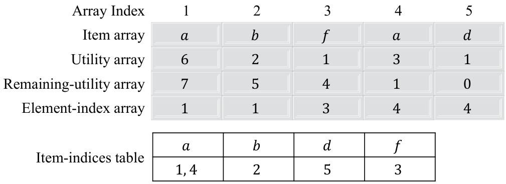
Definition 4.6.
(Extension-list) Assuming -sequence of QSDB has instances of sequence with extension positions , , , , where . The extension-list of in consists of elements, where the th element contains the following fields:
- •
Field acu is the utility of with extension position .
- •
Field exIndex is the (the index of the extension item with extension position ).
For example, in Table 1, has three instances of sequence at , and . Thus, the extension-list of in has two elements “acu: , exIndex: 4", and “acu: , exIndex: 6". For the projection database of each LQS-tree node, HUSP-SP introduces the Sequence Projection (seqPro) structure to represent the -sequence. The seqPro structure is composed of two fields:
- •
Seq-array: This is a pointer to the original seq-array of the -sequence.
- •
Extension-list: It is a list that records the indices of extension items and the sequence utilities with extension positions of the current node pattern.
Compared to the projection database structure, such as UL-lists proposed in HUSP-ULL (Gan et al. 2021c), the seqPro is more refined in modeling the -sequence. Furthermore, with the newly introduced item-index head table, seqPro avoids the problem of storing lots of null values in UL-lists. Additionally, the introduced Extension-list makes seqPro more useful in facilitating pattern generation and utility calculation.
According to Definition 3.5, the utility of a pattern in a -sequence is the maximum utility of all the pattern instances in the -sequence, and the pattern utility is the sum of all the pattern utilities of -sequences in the QSDB that contain the pattern. Obviously, it is time-consuming for the utility calculation for each candidate pattern to find all the instances by scanning the sequences, then compute the utility of each instance, select the maximum utilities, and sum them up at last. Thanks to pattern growth and the database projection methods, the utility computation complexity of child nodes is greatly reduced by recording the location and utility of the parent node pattern’s instances (extension-list). For example, in Table 1, the utility calculation process of sequence can be described as follows. First, although the prefix sequence is contained in every -sequence in the database, only needs to be considered since only contains . Next, the utility of can be efficiently calculated in projected database based on the recorded instances of . Specifically, the sequence can be formed by appending item to instances of with extension positions 1 and 2, respectively. Notice that as there is only one extension item of in , = = , + = + 3 = 4. Furthermore, the extension-list of is constructed for facilitating the candidate items discovery, utility calculation, and upper bound calculation of newly generated super-sequences.
4.3. Search Space Pruning
To reduce the search space, HUSP-SP not only adopts the utility upper bounds (prefix extension utility (PEU) (Wang et al. 2016), and reduced sequence utility (RSU) (Wang et al. 2016)) but also proposes a new utility upper bound, called tighter reduced sequence utility (TRSU). Furthermore, based on these upper bounds, several powerful pruning strategies are designed in HUSP-SP.
Definition 4.7.
(PEU (Wang et al. 2016)) The PEU of sequence in -sequence with extension position is defined as
| (4) |
The PEU of sequence in is defined as
| (5) |
Note, PEU() = when is null. Moreover, the PEU of sequence in QSDB is defined as
| (6) |
For example, int Table 1, = + + + = 8 + 5 + 8 + 8 = 29.
Theorem 4.8.
For any extension of sequence in database with a sequence (not null), = , PEU() (Wang et al. 2016).
Proof.
Let , be the set of -sequences containing and , respectively, we have . For each -sequence , = , we will proof the theorem by proofing that . Assuming = , , , , , then there is always
| (7) |
| (8) |
Observing the Eq. 7 and Eq. 8, it’s obviously that , , , , and the /, i.e., , , , , . Therefore, . According to the Eq. 5, . Thus, PEU( and PEU(, i.e. PEU(. In the same way, PEU() when = . ∎
Theorem 4.8 indicates that, for any QSDB , the candidate sequences with low PEUs (less than ) can be pruned by HUSP-SP since the utilities of all these candidate sequences and their extension sequences will be no greater than the PEUs.
Definition 4.9.
(RSU (Wang et al. 2016)) Let sequence be generated by one item Extension from sequence . The RSU of in -sequence is defined as
| (9) |
Accordingly, the RSU of the sequence in the database is defined as
| (10) |
Note, if is a single item sequence, then is the same to the commonly known sequence-weighted utilization (SWU) (Yin et al. 2012), since = .
For example, in Table 1, = RSU() + RSU() = PEU() + PEU( = 6 + 10 = 16.
Theorem 4.10.
For any Extension of sequence in database with sequence , which can be empty, = , (Yin et al. 2013).
Proof.
HUSP-SP can efficiently calculate the RSU of the newly generated candidate pattern by adding the PEU values of -sequences that still contain the new pattern. Then, according to Theorem 4.10, HUSP-SP can prune the candidates with low RSU values (less than ). However, RSU only utilizes the PEU of the prefix sequence for fast calculation, ignoring the help of the newly added item to reduce the utility upper bound. For instance, the sequence generates by one item extension, and = PEU() + PEU( = 6 + 10 = 16. PEU( = , where the subsequence between b and e, , is irrelevant to the candidate pattern and ’s extended sequences but contributes to the utility upper bound of . The same problem can be found in PEU(). Therefore, we designed a new tighter utility upper bound TRSU to overcome the disadvantages of RSU by considering the newly added item and subtracting the utility value of the irrelevant subsequence from the PEU under certain conditions. We shall learn later that the value of is , and it is much less than the value of , 16.
Definition 4.11.
(TRSU) Assuming -sequence of QSDB has instances of sequence with extension positions , , , , where . Let sequence be generated by one item Extension from sequence . The TRSU of in -sequence is defined as
| (11) |
where is the first extension position of , represents the first extension position of , and is the first extension position of before ( may equal to ) in . Also, the TRSU of the sequence in database is defined as
| (12) |
For example, in Table 1, = + = - - + - - = 6 - (5 - 3) + 10 - (8 - 1) = 7. Besides, as the example in Definition 4.9 states, the = 16, which is even greater than twice the value of . It shows the TRSU is much tighter than the RSU. Note that the TRSU and RSU are the same kinds of upper bounds that are designed based on the look-ahead strategy (Lin et al. 2017). Besides, TRSU provides an idea for further reducing the upper bounds designed based on the look-ahead strategy.
Theorem 4.12.
For any Extension of sequence in the database with sequence , can be empty, = , .
Proof.
Assuming is generated by one item Extension from sequence , = , then = . Let , and be the set of -sequences containing , and respectively, we have . According to Definition 4.11, there are two scenarios for the computation of for each -sequence . On the one hand, when = + , = - - , where is the first extension position of , is the first extension position of , and is the first extension position of before . According to THEOREM 4.10, , and it can be observed that the sub -sequence of from index to is irrelevant to any (there will be no subsequence of contained in this sub -sequence). Therefore, - , since the contains the utility of the irrelevant sub -sequence, that’s to say, TRSU(). On the other hand, TRSU() = RSU() = PEU(), and we have . Hence, TRSU() also holds. In conclusion, TRSU(), , i.e., . ∎
HUSP-SP can also efficiently calculate the TRSU of newly generated candidate patterns with the help of the remaining-utility array. According to THEOREM 4.12, HUSP-SP can prune the candidates with low TRSU values (less than ). Based on the utility upper bounds, the pruning strategies are described as follows. First, the IIP (irrelevant items pruning) strategy (Gan et al. 2021c) is adopted by HUSP-SP, and it is defined based on RSU in this paper as follows. IIP Strategy: Given a sequence , and any item available for extension, if RSU( is less than the minimum utility threshold ( ), then can be removed from the seqPro structure of and ’s extension sequences. The correctness of the IIP strategy and proof process have been given in HUSP-ULL (Gan et al. 2021c). Then, according to THEOREM 4.12, an EP (early pruning) strategy is proposed to discard unpromising candidate items early. EP Strategy: Given a sequence and any item available for extension, two situations are considered: 1). If is an I-Extension candidate item, and TRSU( , then should be discarded. 2). If is an S-Extension candidate item, and TRSU( , then should be discarded.
4.4. HUSP-SP Algorithm
Based on the seq-array, the designed TRSU, and the EP strategy, the proposed HUSP-SP algorithm can be stated as follows. Algorithm 1 gives the main steps of HUSP-SP. The algorithm first scans the quantitative sequential database to construct the storage structure, that is, the seq-array of each -sequence (line 1). It also accumulates the utility of the -sequences and gets the after scanning the database (line 1). Then, the projected database seqPro() of the empty sequence is constructed (lines 3-4). Following that, the empty sequence is treated as the prefix, and HUSP-SP begins the depth-first search with the built projected database by invoking the PatternGrowth procedure (line 5).
The PatternGrowth procedure (cf. Algorithm 2) shows the depth-first search process, i.e., the pattern growth process through the I-Extension and S-Extension operations. The algorithm first removes the irrelevant items from the projected database by applying the IIP strategy, and then updates the projected database, seqPro(prefix) (line 1). Then, the reduced projected database seqPro(prefix) is scanned to get the promising I-Extension items (iList) and S-Extension items (sList) of prefix by EP strategy (line 2). For each item of iList and sList, the algorithm generates a new one length longer pattern by applying I-Extension and S-Extension with , respectively. Furthermore, the newly generated pattern, such as prefix , is evaluated by calling the UtilityCalculation procedure (lines 3-8).
The UtilityCalculation procedure (cf. Algorithm 3) first establishes the seq-array field of the projected database seqPro(prefix′) based on the seqPro(prefix) (line 1). Then, the utility and PEU value of prefix′ are calculated based on the constructed seqPro(prefix′); meanwhile, the Extension-List field of the seqPro(prefix′) is built (line 2). If the (prefix′) is not less than the minimum utility , the prefix′ is added to the HUSPs (lines 3-5). Furthermore, if the PEU(prefix′) is not less than , the PatternGrowth procedure is called to mine the HUSPs prefixed with prefix′ (lines 6-8). Note, the utilization of PEU can result in missing patterns when the pruning condition “if PEU(prefix′) then stop the mining branch with prefix′ as parent node" is executed before displaying the result sequence “if ( ) then output prefix′" (Truong-Chi and Fournier-Viger 2019). Finally, HUSP-SP terminates when there are no newly generated candidate patterns, and returns the set of HUSP, HUSPs.
To better illustrate the proposed algorithm, we give a running example below. Considering the running example (Table 1 and Table ), and = 0.5. After the first scanning of the database, we build the seq-arrays for -sequences of the database and obtain that the threshold value is = 23.5, the SWU (Yin et al. 2012) value of , , , , , are 29, 35, 12, 47, 34, 31. Thus, the item is permanently deleted from the database as its SWU value is less than the threshold value. Then we get the TRSU value of , , , , are 29, 23, 22, 10, and 10 by scanning the original seq-arrays. So, is the only promising candidate. Next, we scan the original seq-arrays again to construct the projected database (seqPros) and calculate the utility of . The utility and PEU values of are and , separately. Therefore, is not a HUSP, and we should call the PatternGrowth on it for mining its extension sequences. Firstly, we get the RSU value of and are 16 and 13 by searching the seqPro of . Thus, we delete the items and from the seqPro of based on the IIP strategy. Then, we scan the reduced seqPro(), and we find two I-Extension sequences and , whose TRSU value are and . The S-Extension sequences of include and , whose TRSU value are and . According to the EP strategy, we can discard the as its TRSU value is less than 23.5. , and are the promising candidates, and we call the UtilityCalculation for each of them. The mining process for and is terminated since their PEU values are 17 and 19. The utility and PEU values of are 16 and 27, so is not a HUSP. Finally, we call the PatternGrowth on and get one HUSP with a utility of 25.
4.5. Complexity Analysis
Let denotes the number of -sequences in database , denotes the length of the longest -sequence in , and denotes the number of distinct items in . HUSP-SP first scans the database to build the seq-arrays, whose time complexity is . The memory complexity of the seq-arrays is also since there are seq-arrays, and the most extended length is . Then, HUSP-SP calls the recursive function PatternGrowth after some initial operations and finally returns the HUSPs. Thus, the time complexity of the HUSP-SP algorithm is + , where denotes the number of times PatternGrowth is called, and denotes the time complexity of PatternGrowth. The memory complexity of HUSP-SP is + , where H denotes the maximum depth of recursively calling PatternGrowth, denotes the memory complexity of PatternGrowth.
As for PatternGrowth, the procedure first needs to scan the projected database three times (lines 1-2), whose worst time complexity is . Specifically, the IIP operation first takes one scan to mark the extension items with low RSU as irrelevant items, and then scans the projected database again to update the projected database by deleting the utility of the irrelevant items in the Remaining-utility array (Definition 4.5). After the IIP operation, PatternGrowth scans the reduced projected database once to get the promising extension items, iList and sList. The remaining operations of PatternGrowth are appending each item of iList or sList to the prefix and calculating the utility of the generated candidate pattern (lines 3-8), whose worst time complexity is . Note that the represents the time complexity of UtilityCalculation. Thus, the worst time complexity of PatternGrowth is + . In addition, the worst memory complexity of PatternGrowth is + . This is because the largest size of the projected database can be when each -sequence in contains the candidate pattern. Moreover, the largest size of Extension-list can be when the candidate pattern is equal to any subsequence of the same length in . Therefore, the worst memory complexity of the projected database can be . In addition, for marking deleted items, the IIP operation requires a global array of length .
Additionally, the worst time complexity of the UtilityCalculation is . This is because the projected database may contain at most -sequences. Besides, for each -sequence, calculating the utility of the new candidate pattern needs to traverse the extension-List and Item-indices table, which may contain at most elements. According to the above, the value of timeComp_UC is , and the value of timeComp_PG is + , which equals . Thus, the time complexity of the HUSP-SP algorithm is + , which equals . Besides, the value of memoComp_PG is , and the memory complexity of HUSP-SP is + + , which equals . Note that there is only one global array of length for marking deleted items; thus, the factor of is one instead of . To sum up, the time complexity of the HUSP-SP algorithm is , and the memory complexity is .
It is worth noting that the number of candidate patterns (LQS-tree nodes) is , which is equal to the value of . Furthermore, the length of the longest pattern is , which equals the value of . Therefore, the worst time complexity and memory complexity of the HUSP-SP algorithm are and , separately. Nevertheless, the exact time and memory complexity of HUSP-SP can be much smaller than the above theoretical values, as the proposed pruning strategies can significantly reduce the search space (the number of candidate patterns).
5. Experiments
In this section, sufficient experimental results were presented and analyzed to demonstrate the performance of the proposed algorithm. The state-of-the-art HUSPM algorithms, including USpan (Yin et al. 2012) (replaced the SPU by PEU), ProUM (Gan et al. 2020b) and HUSP-ULL (Gan et al. 2021c) were selected as the baselines. All the compared algorithms were implemented in Java. All the course code and datasets are available at GitHub11 1 https://github.com/DSI-Lab1/HUSPM. The following experiments were conducted on a personal computer with an Intel Core i7-8700K CPU @ 3.20 GHz, a 3.19 GHz processor, 8 GB of RAM, and a 64-bit Windows 10 operating system.
5.1. Data Description
Five real-world datasets and one synthetic dataset were utilized in our experiment to evaluate the performance of the compared algorithms. Table 2 lists the statistical characteristics of these datasets. Note that the number of -sequences is denoted as , the number of different -items is denoted as , the average/maximum length of -sequences is denoted as /, the average number of -itemsets per -sequence is denoted as #avg(IS), the average number of -items per -itemset is denoted as #Ele, and the average/maximum utility of -items is denoted as avg(UI)/max(UI). The values of #Ele parameter of these datasets indicate that the Sign, Bible, Kosarak10k and Leviathan are composed of single item element based sequences, while the Yoochoose and SynDataset-160K are composed of multi-item element based sequences. The utilization of both single-item and multi-item element based sequence datasets makes the experimental results more convincing. Excluding Yoochoose22 2 https://recsys.acm.org/recsys15/challenge, the other datasets can be obtained from an open-source data mining website33 3 http://fimi.ua.ac.be/data.
| Dataset | avg(IS) | #Ele | ||||
|---|---|---|---|---|---|---|
| Sign | 730 | 267 | 52.00 | 94 | 52.00 | 1.00 |
| Bible | 36,369 | 13,905 | 21.64 | 100 | 21.64 | 1.00 |
| SynDataset-160k | 159,501 | 7,609 | 6.19 | 20 | 26.64 | 4.32 |
| Kosarak10k | 10,000 | 10,094 | 8.14 | 608 | 8.14 | 1.00 |
| Leviathan | 5,834 | 9,025 | 33.81 | 100 | 33.81 | 1.00 |
| Yoochoose | 234,300 | 16,004 | 2.25 | 112 | 1.14 | 1.98 |
| SynDataset-10k | 10,000 | 7,312 | 27.11 | 213 | 6.23 | 4.35 |
| SynDataset-80k | 79,718 | 7,584 | 26.80 | 213 | 6.20 | 4.32 |
| SynDataset-160k | 159,501 | 7,609 | 26.75 | 213 | 6.19 | 4.32 |
| SynDataset-240k | 239,211 | 7,617 | 26.77 | 213 | 6.19 | 4.32 |
| SynDataset-320k | 318,889 | 7,620 | 26.76 | 213 | 6.19 | 4.32 |
| SynDataset-400k | 398,716 | 7,621 | 26.75 | 213 | 6.19 | 4.32 |
5.2. Efficiency Analysis
In the first experiment, the runtime performance of the proposed algorithm was compared with the state-of-the-art algorithms. Then, on six datasets, a series of experiments with various minimum utility threshold (denoted as ) settings were run, with the detailed results shown in Fig. 3.
It is shown that the proposed HUSP-SP is faster than the other existing algorithms in all cases. Generally, HUSP-SP was a quarter faster than the state-of-the-art algorithm HUSP-ULL, one order of magnitude faster than ProUM, and two or three orders of magnitude faster than USpan. For example, except for the SynDataset-160k in Fig. 3(c), the runtime of HUSP-SP consumes around ten seconds, while the other algorithms may consume hundreds to thousands of seconds. Furthermore, HUSP-SP and HUSP-ULL are much more stable than ProUM and USpan in runtime efficiency when decreases. For instance, in Fig. 3(c), the runtime of USpan and ProUM increased by a hundred seconds when decreased by 0.00005, while HUSP-SP ran only a few seconds longer. Note that when the minimum threshold parameter is less than on the Leviathan dataset, the USpan algorithm cannot finish the experiment because it has run out of memory. In all parameter settings, HUSP-SP is superior to all existing algorithms.
5.3. Effectiveness of Pruning Strategies
In order to evaluate the effect of pruning strategies, this subsection investigated the generated candidate patterns and HUSPs of the compared algorithms under varying minimum utility thresholds in the six datasets. The details are shown in Fig. 4. Note that #candidate is the number of the generated candidate patterns, which must be checked, and #HUSPs is the number of the final HUSPs discovered by the method.
As shown in Fig. 4, the number of candidate patterns generated by HUSP-ULL and HUSP-SP is much smaller than the other two methods. The main reason for the huge difference in the number of candidates is that HUSP-ULL and HUSP-SP adopt the IIP strategy. With the introduction of the IIP strategy, the utility upper bounds decreased faster due to the utility deletion of irrelevant items. Therefore, the search space was much smaller when the IIP strategy worked. Besides, HUSP-SP generally generates half as many candidate patterns as HUSP-ULL. Therefore, it proves that the proposed new upper bound TRSU and the EP pruning strategy are effective.
It can also be observed that the number of candidate patterns of HUSP-SP and HUSP-ULL increased much slower than USpan and ProUM. However, Fig. 4(f) shows that, in the dataset Yoochoose, the compared algorithms generated a similar number of candidate patterns. Still, from Fig. 3 and Fig. 5, we can find that the proposed HUSP-SP performed better in terms of runtime and memory. Therefore, the proposed projected structure seqPro is more compact and more effective in the HUSP mining process.
5.4. Memory Evaluation
In this subsection, the important algorithmic measure criteria for memory are evaluated. The experiment results are shown in Fig. 5.
HUSP-SP outperformed all of the compared algorithms in terms of memory consumption across all experiment parameter settings, as shown in Fig. 5. It can be observed that the memory usage of the HUSPM method increased when the number of candidate patterns increased. For example, Fig. 5(d) shows that USpan (ProUM) consumed about 600 megabytes more memory than HUSP-SP (HUSP-ULL), while USpan (ProUM) generated over 100,000,000 more candidate patterns than HUSP-SP (HUSP-ULL). The memory performance of USpan is generally poor. For instance, USpan ran out of memory when the minimum utility threshold was less than 1.20% in Leviathan. Also, it can be found that the data structures utilized by ProUM and HUSP-ULL are not compact enough in some conditions. For example, in Fig. 5(a), the USpan consumed about 200 megabytes less memory than ProUM and HUSP-ULL. However, the performance of the utility-matrix (Yin et al. 2012) utilized by USpan was poor. In conclusion, the good memory usage performance of HUSP-SP proves that the newly proposed seq-array structure is compact, and the search space of HUSP-SP is much smaller.
5.5. Scalability Test
The robustness of the compared algorithms is analyzed in this subsection through the scalability test. The experiment was based on a synthetic multi-item element-based sequence dataset, namely C8S6T4I3D|X|K (Agrawal and Srikant 1994). The detailed results are shown in Fig. 6, including runtime, candidate, and memory efficiency. Note that the size of the SynDataset varied from 10K to 400K sequences, and the minimum utility threshold was set to 0.001 throughout the experiment.
As shown in Fig. 6, HUSP-SP had the best scalability among the compared algorithms for its minimum runtime, memory consumption, and candidate pattern number in all the test results. Furthermore, the runtime of HUSP-SP increased linearly as the number of dataset sequences grew. From Fig. 6(b), it can be observed that the memory usage of HUSP-SP is relatively stable, excluding the experiment with 10K sequences. Similar results can be found in Fig. 6(c) where the number of candidate patterns was kept stable while the size of SynDataset varied from 80K to 400K. Therefore, the growth in memory usage of HUSP-SP comes mainly from the expansion of the processed dataset. The proposed HUSP-SP algorithm has good extensibility for dealing with large-scale datasets.
5.6. Ablation Study
We further conducted an ablation study on the proposed upper bound TRSU to evaluate its effects on execution performance in terms of runtime, memory consumption, and the number of generated candidates. Theoretically, introducing TRSU can reduce the search space and speed up the mining process. To evaluate the effectiveness of TRSU, we developed another algorithm, HUSP-SP*, by replacing the upper bound of HUSP-SP from TRSU to RSU. We examined two datasets, SynDataset80k and SynDataset160k, with different minimum utility threshold settings. The detailed study results are shown in Fig. 7.
As we can see, HUSP-SP has a shorter runtime and fewer candidate patterns in all cases of the study results. It proves that TRSU does contribute to the high performance of HUSP-SP. It is interesting that HUSP-SP and HUSP-SP* have the same memory consumption result in all cases. To explain this phenomenon, we perform a further experiment and find that when we continually change the minimum utility threshold, e.g., set to 0.0004, the memory consumption of HUSP-SP on SynDataset80K increases to 750 MB, and the candidate number increases to 7,888,232. That is to say, the number of candidates increased by nearly 8,000,000 while memory consumption increased by less than 100 MB. Besides, in all the study cases in Fig. 7, we can find that the number of candidates varies by no more than 100,000. Therefore, it reflects that the memory consumption results are the same within a dataset. Furthermore, it demonstrates the stability of the proposed HUSP-SP: its memory consumption performance is not as sensitive to changes in . From the study result comparison between datasets SynDataset80K and SynDataset160K, we can also find that HUSP-SP has good scalability in terms of database size. In conclusion, the proposed upper bound TRSU significantly contributes to improving the efficiency of the algorithms.
6. Conclusion
Due to its more comprehensive consideration of the sequence data, database-based sequence mining has played an important role in the domain of knowledge discovery in databases. In general, utility mining takes frequency, sequential order, and utility into consideration, while the combinatorial explosion of sequences and utility computation make utility mining a NP-hard problem. This article proposes a novel HUSP-SP algorithm that addresses the problem more efficiently than the existing methods. HUSP-SP developed the compact seq-arrays to store the necessary information from sequence data. Besides, the projected database structure, namely seqPro was designed to efficiently calculate the utilities and upper bound values of candidate patterns. Furthermore, a new tight utility upper bound, namely TRSU, and two search space pruning strategies are proposed to improve the mining performance of HUSP-SP. Extensive experimental results on both synthetic and real-life datasets show that the HUSP-SP algorithm outperforms the state-of-the-art algorithms, e.g., HUSP-ULL. In the future, an interesting direction is to redesign HUSP-SP and develop a parallel and distributed version, for example, utilizing MapReduce or Spark to discover the interesting HUSPs on large-scale databases in distributed environments.
Acknowledgment
This research was supported in part by the National Natural Science Foundation of China (Nos. 62002136 and 62272196), Natural Science Foundation of Guangdong Province (Nos. 2020A1515010970 and 2022A1515011861), Shenzhen Research Council (No. GJHZ20180928155209705), and NSF Grants (Nos. III-1763325, III-1909323, and SaTC-1930941).
References
- (1)
- Agrawal and Srikant (1994) R. Agrawal and R. Srikant. 1994. Quest synthetic data generator. (1994). http://www.Almaden.ibm.com/cs/quest/syndata.html
- Agrawal and Srikant (1995) Rakesh Agrawal and Ramakrishnan Srikant. 1995. Mining sequential patterns. In The 7th International Conference on Data Engineering. IEEE, 3–14.
- Agrawal et al. (1994) Rakesh Agrawal, Ramakrishnan Srikant, et al. 1994. Fast algorithms for mining association rules. In The 20th International Conference Very Large Data Bases. 487–499.
- Ahmed et al. (2010a) Chowdhury Farhan Ahmed, Syed Khairuzzaman Tanbeer, and Byeong-Soo Jeong. 2010a. Mining high utility web access sequences in dynamic web log data. In 11th ACIS International Conference on Software Engineering, Artificial Intelligence, Networking and Parallel/Distributed Computing. IEEE, 76–81.
- Ahmed et al. (2010b) Chowdhury Farhan Ahmed, Syed Khairuzzaman Tanbeer, and Byeong-Soo Jeong. 2010b. A novel approach for mining high-utility sequential patterns in sequence databases. ETRI Journal 32, 5 (2010), 676–686.
- Ahmed et al. (2009) Chowdhury Farhan Ahmed, Syed Khairuzzaman Tanbeer, Byeong-Soo Jeong, and Young-Koo Lee. 2009. Efficient tree structures for high utility pattern mining in incremental databases. IEEE Transactions on Knowledge and Data Engineering 21, 12 (2009), 1708–1721.
- Alkan and Karagoz (2015) Oznur Kirmemis Alkan and Pinar Karagoz. 2015. CRoM and HuspExt: Improving efficiency of high utility sequential pattern extraction. IEEE Transactions on Knowledge and Data Engineering 27, 10 (2015), 2645–2657.
- Bejerano and Yona (1999) Gill Bejerano and Golan Yona. 1999. Modeling protein families using probabilistic suffix trees. In The 3th Annual International Conference on Computational Molecular Biology. 15–24.
- Brin et al. (1997) Sergey Brin, Rajeev Motwani, Jeffrey D Ullman, and Shalom Tsur. 1997. Dynamic itemset counting and implication rules for market basket data. In The ACM SIGMOD International Conference on Management of Data. 255–264.
- Chan et al. (2003) Raymond Chan, Qiang Yang, and Yi-Dong Shen. 2003. Mining high utility itemsets. In The 3th IEEE International Conference on Data Mining. IEEE, 19–19.
- Chen et al. (1996) Ming-Syan Chen, Jiawei Han, and Philip S. Yu. 1996. Data mining: An overview from a database perspective. IEEE Transactions on Knowledge and Data Engineering 8, 6 (1996), 866–883.
- Dam et al. (2019) Thu-Lan Dam, Kenli Li, Philippe Fournier-Viger, and Quang-Huy Duong. 2019. CLS-Miner: efficient and effective closed high-utility itemset mining. Frontiers of Computer Science 13, 2 (2019), 357–381.
- Fournier-Viger et al. (2022) Philippe Fournier-Viger, Wensheng Gan, Youxi Wu, Mourad Nouioua, Wei Song, Tin Truong, and Hai Duong. 2022. Pattern Mining: Current Challenges and Opportunities. In Proceedings of the 27th International Conference on Database Systems for Advanced Applications Workshops. Springer, 34–49.
- Fournier-Viger et al. (2017) Philippe Fournier-Viger, Jerry Chun-Wei Lin, Rage Uday Kiran, Yun Sing Koh, and Rincy Thomas. 2017. A survey of sequential pattern mining. Data Science and Pattern Recognition 1, 1 (2017), 54–77.
- Fournier-Viger et al. (2014) Philippe Fournier-Viger, Cheng-Wei Wu, Souleymane Zida, and Vincent S Tseng. 2014. FHM: Faster high-utility itemset mining using estimated utility co-occurrence pruning. In International Symposium on Methodologies for Intelligent Systems. Springer, 83–92.
- Gan et al. (2021a) Wensheng Gan, Zilin Du, Weiping Ding, Chunkai Zhang, and Han Chieh Chao. 2021a. Explainable fuzzy utility mining on sequences. IEEE Transactions on Fuzzy Systems 29, 12 (2021), 3620–3634.
- Gan et al. (2019b) Wensheng Gan, Jerry Chun-Wei Lin, Han-Chieh Chao, Hamido Fujita, and Philip S Yu. 2019b. Correlated utility-based pattern mining. Information Sciences 504 (2019), 470–486.
- Gan et al. (2018a) Wensheng Gan, Jerry Chun-Wei Lin, Han-Chieh Chao, Shyue-Liang Wang, and Philip S Yu. 2018a. Privacy preserving utility mining: a survey. In IEEE International Conference on Big Data. IEEE, 2617–2626.
- Gan et al. (2019a) Wensheng Gan, Jerry Chun Wei Lin, Han Chieh Chao, and Philip S Yu. 2019a. Utility-driven mining of high utility episodes. In IEEE International Conference on Big Data. IEEE, 2644–2653.
- Gan et al. (2018b) Wensheng Gan, Jerry Chun Wei Lin, Philippe Fournier-Viger, Han Chieh Chao, Tzung Pei Hong, and Hamido Fujita. 2018b. A survey of incremental high-utility itemset mining. Wiley Interdisciplinary Reviews: Data Mining and Knowledge Discovery 8, 2 (2018), e1242.
- Gan et al. (2021b) Wensheng Gan, Jerry Chun Wei Lin, Philippe Fournier-Viger, Han Chieh Chao, Vincent S Tseng, and Philip S Yu. 2021b. A survey of utility-oriented pattern mining. IEEE Transactions on Knowledge and Data Engineering 33, 4 (2021), 1306–1327.
- Gan et al. (2019c) Wensheng Gan, Jerry Chun Wei Lin, Philippe Fournier-Viger, Han Chieh Chao, and Philip S Yu. 2019c. A survey of parallel sequential pattern mining. ACM Transactions on Knowledge Discovery from Data 13, 3 (2019), 1–34.
- Gan et al. (2020b) Wensheng Gan, Jerry Chun-Wei Lin, Jiexiong Zhang, Han-Chieh Chao, Hamido Fujita, and Philip S Yu. 2020b. ProUM: Projection-based utility mining on sequence data. Information Sciences 513 (2020), 222–240.
- Gan et al. (2021c) Wensheng Gan, Jerry Chun-Wei Lin, Jiexiong Zhang, Philippe Fournier-Viger, Han-Chieh Chao, and Philip S Yu. 2021c. Fast utility mining on sequence data. IEEE Transactions on Cybernetics 51, 2 (2021), 487–500.
- Gan et al. (2021d) Wensheng Gan, Jerry Chun Wei Lin, Jiexiong Zhang, Hongzhi Yin, Philippe Fournier-Viger, Han Chieh Chao, and Philip S Yu. 2021d. Utility mining across multi-dimensional sequences. ACM Transactions on Knowledge Discovery from Data 15, 5 (2021), 1–24.
- Gan et al. (2020a) Wensheng Gan, Jerry Chun-Wei Lin, Jiexiong Zhang, and Philip S Yu. 2020a. Utility mining across multi-sequences with individualized thresholds. ACM Transactions on Data Science 1, 2 (2020), 1–29.
- Han et al. (2001) Jiawei Han, Jian Pei, Behzad Mortazavi-Asl, Helen Pinto, Qiming Chen, Umeshwar Dayal, and Meichun Hsu. 2001. PrefixSpan: Mining sequential patterns efficiently by prefix-projected pattern growth. In The 17th International Conference on Data Engineering. Citeseer, 215–224.
- Han et al. (2004) Jiawei Han, Jian Pei, Yiwen Yin, and Runying Mao. 2004. Mining frequent patterns without candidate generation: A frequent-pattern tree approach. Data Mining and Knowledge Discovery 8, 1 (2004), 53–87.
- Jindal and Liu (2006) Nitin Jindal and Bing Liu. 2006. Identifying comparative sentences in text documents. In The 29th Annual International ACM SIGIR Conference on Research and Development in Information Retrieval. 244–251.
- Lin et al. (2016) Jerry Chun-Wei Lin, Wensheng Gan, Philippe Fournier-Viger, Tzung-Pei Hong, and Vincent S Tseng. 2016. Efficient algorithms for mining high-utility itemsets in uncertain databases. Knowledge-Based Systems 96 (2016), 171–187.
- Lin et al. (2017) Jerry Chun-Wei Lin, Jiexiong Zhang, and Philippe Fournier-Viger. 2017. High-utility sequential pattern mining with multiple minimum utility thresholds. In Asia-Pacific Web (APWeb) and Web-Age Information Management (WAIM) Joint Conference on Web and Big Data. Springer, 215–229.
- Liu and Qu (2012) Mengchi Liu and Junfeng Qu. 2012. Mining high utility itemsets without candidate generation. In The 21st ACM International Conference on Information and Knowledge Management. 55–64.
- Liu et al. (2005) Ying Liu, Wei-Keng Liao, and Alok Choudhary. 2005. A two-phase algorithm for fast discovery of high utility itemsets. In Pacific-Asia Conference on Knowledge Discovery and Data Mining. Springer, 689–695.
- Shie et al. (2012) Bai-En Shie, Philip S Yu, and Vincent S Tseng. 2012. Efficient algorithms for mining maximal high utility itemsets from data streams with different models. Expert Systems with Applications 39, 17 (2012), 12947–12960.
- Srivastava et al. (2021) Gautam Srivastava, Jerry Chun Wei Lin, Xuyun Zhang, and Yuanfa Li. 2021. Large-scale high-utility sequential pattern analytics in Internet of things. IEEE Internet of Things Journal 8, 16 (2021), 12669 –12678.
- Truong et al. (2019) Tin Truong, Hai Duong, Bac Le, and Philippe Fournier-Viger. 2019. FMaxCloHUSM: An efficient algorithm for mining frequent closed and maximal high utility sequences. Engineering Applications of Artificial Intelligence 85 (2019), 1–20.
- Truong-Chi and Fournier-Viger (2019) Tin Truong-Chi and Philippe Fournier-Viger. 2019. A survey of high utility sequential pattern mining. In High-Utility Pattern Mining. Springer, 97–129.
- Tseng et al. (2013) Vincent S Tseng, Bai En Shie, Cheng Wei Wu, and Philip S Yu. 2013. Efficient algorithms for mining high utility itemsets from transactional databases. IEEE Transactions on Knowledge and Data Engineering 25, 8 (2013), 1772–1786.
- Tseng et al. (2015) Vincent S Tseng, Cheng-Wei Wu, Philippe Fournier-Viger, and Philip S Yu. 2015. Efficient algorithms for mining top- high utility itemsets. IEEE Transactions on Knowledge and Data Engineering 28, 1 (2015), 54–67.
- Tseng et al. (2010) Vincent S Tseng, Cheng-Wei Wu, Bai-En Shie, and Philip S Yu. 2010. UP-Growth: An efficient algorithm for high utility itemset mining. In The 16th ACM SIGKDD International Conference on Knowledge Discovery and Data Mining. 253–262.
- Van et al. (2018) Trang Van, Bay Vo, and Bac Le. 2018. Mining sequential patterns with itemset constraints. Knowledge and Information Systems 57, 2 (2018), 311–330.
- Wang and Huang (2018) Jun Zhe Wang and Jiun Long Huang. 2018. On incremental high utility sequential pattern mining. ACM Transactions on Intelligent Systems and Technology 9, 5 (2018), 1–26.
- Wang et al. (2016) Jun-Zhe Wang, Jiun-Long Huang, and Yi-Cheng Chen. 2016. On efficiently mining high utility sequential patterns. Knowledge and Information Systems 49, 2 (2016), 597–627.
- Wu et al. (2021) Youxi Wu, Rong Lei, Yan Li, Lei Guo, and Xindong Wu. 2021. HAOP-Miner: Self-adaptive high-average utility one-off sequential pattern mining. Expert Systems with Applications 184 (2021), 115449.
- Xu et al. (2017) Tiantian Xu, Xiangjun Dong, Jianliang Xu, and Xue Dong. 2017. Mining high utility sequential patterns with negative item values. International Journal of Pattern Recognition and Artificial Intelligence 31, 10 (2017), 1750035.
- Yin et al. (2012) Junfu Yin, Zhigang Zheng, and Longbing Cao. 2012. USpan: An efficient algorithm for mining high utility sequential patterns. In The 18th ACM SIGKDD International Conference on Knowledge Discovery and Data Mining. 660–668.
- Yin et al. (2013) Junfu Yin, Zhigang Zheng, Longbing Cao, Yin Song, and Wei Wei. 2013. Efficiently mining top- high utility sequential patterns. In The 13th International Conference on Data Mining. IEEE, 1259–1264.
- Zhang et al. (2022) Chunkai Zhang, Quanjian Dai, Zilin Du, Wensheng Gan, Jian Weng, and Philip S Yu. 2022. TUSQ: Targeted high-utility sequence querying. IEEE Transactions on Big Data. DOI: 10.1109/TBDATA.2022.3175428 (2022), 1–14.
- Zhang et al. (2021a) Chunkai Zhang, Zilin Du, Wensheng Gan, and Philip S Yu. 2021a. TKUS: Mining top- high utility sequential patterns. Information Sciences 570 (2021), 342–359.
- Zhang et al. (2021b) Chunkai Zhang, Zilin Du, Yuting Yang, Wensheng Gan, and Philip S Yu. 2021b. On-shelf utility mining of sequence data. ACM Transactions on Knowledge Discovery from Data 16, 2 (2021), 1–31.
- Zida et al. (2015) Souleymane Zida, Philippe Fournier-Viger, Jerry Chun Wei Lin, Cheng Wei Wu, and Vincent S Tseng. 2015. EFIM: a highly efficient algorithm for high-utility itemset mining. In Mexican International Conference on Artificial Intelligence. Springer, 530–546.
- Zihayat et al. (2017) Morteza Zihayat, Yan Chen, and Aijun An. 2017. Memory-adaptive high utility sequential pattern mining over data streams. Machine Learning 106, 6 (2017), 799–836.