Intersecting ellipses induced by a max-sum matchingThanks: A.P. is supported by the Bulgarian Ministry of Education and Science, Scientific Programme ”Enhancing the Research Capacity in Mathematical Sciences (PIKOM)”, No. DO1-67/05.05.2022, and by the grant of Russian Science Foundation №22-11-00131, https://rscf.ru/project/22-11-00131/. Also, A.P. is a Young Russian Mathematics award winner and would like to thank its sponsors and jury.

For the sake of brevity, we introduce the following notation for the region bounded by an ellipse

where $a$ and $b$ are some points in the plane. Slightly abusing notation, we say that $\mathcal{E}_{\lambda}(ab)$ is an ellipse. Since the factor $\lambda=2/\sqrt{3}$ plays a main role in Conjecture 1, we put

So we can easily restate Conjecture 1 as follows:

Also, we need the notation of lens. For two distinct points $x,y$ in the plane and $\alpha\in(0,\pi)$, denote by $\alpha(xy)$ the so-called $\alpha$-lens for the line segment $xy$, that is,

Next, we state a trivial observation, which we leave without proof.

We refer to [8]*Subsection 9.2 to read about a high-dimensional problem on the intersection of lenses (generalizing Lemma 3 and similar to Conjecture 5).

We recall a standard notation and theorems from convex geometry; see [6]*Chapter 6.

A function $f:\mathbb{R}^{n}\rightarrow\mathbb{R}$ is called convex if it satisfies the inequality

for any two points $x,y\in\mathbb{R}^{d}$ and $0\leq\lambda\leq 1$. The subdifferential $\partial f(x)$ of a convex function $f$ at a point $x\in\mathbb{R}^{n}$ is given by

where $\langle a,b\rangle$ stands for the dot product of $a,b\in\mathbb{R}^{d}$. According to this definition, the set $\partial f(x)$ is convex. A vector $s\in\partial f(x)$ is called a subgradient of $f$ at $x$.

Next, we state two simple properties of convex functions.

We need the following notation to state the next theorem and its corollary. For convex functions $f_{1},\dots,f_{m}:\mathbb{R}^{n}\to\mathbb{R}$, consider the function $f:\mathbb{R}^{n}\to\mathbb{R}$ defined by $f(x)=\max\{f_{1}(x),\dots,f_{m}(x)\}.$ For any point $x\in\mathbb{R}$, we write $I(x)=\{1\leq i\leq m:f_{i}(x)=f(x)\}.$

The key optimization tool we need is the following corollary of Theorems 7, 8, and 9.

In our problem, we apply Proposition 10 to a particular collection of functions and obtain its corollary in the form needed to prove the Fingerhut conjecture.

First, we introduce an auxiliary notation. For two vectors $x$ and $y$, put

Clearly, the vector $\ell_{xy}$ bisects the angle between $x$ and $y$, and moreover, the point $\ell_{xy}$ belongs to the line segment $xy$.

For any distinct points $a$ and $b$, the function $h_{ab}:\mathbb{R}^{2}\to\mathbb{R}$ is defined by

Clearly, it is well-defined and differentiable everywhere except at $a$ and $b$. For a set $\mathcal{M}$ of pairs of distinct points in the plane, the function $h_{\mathcal{M}}:\mathbb{R}^{2}\to\mathbb{R}$ is given by $h_{\mathcal{M}}\coloneqq\max_{ab\in\mathcal{M}}h_{ab}$.

Throughout this section we use the following angular notation. We define the following functions

Essentially, $\measuredangle(x,y)$ is the directed angle between vectors $x$ and $y$ measured in counterclockwise direction and $\angle(x,y)$ is the smallest (non-negative) angle between $x$ and $y$. Clearly, these functions are well-defined. Slightly abusing notation, we will also consider the angles $\measuredangle(m,n)$ and $\angle(m,n)$ for rays $m$ and $n$ emanating from the origin $o$, that is, $\measuredangle(m,n)=\measuredangle(x,y)$ and $\angle(m,n)=\angle(x,y)$, where $x\in m$ and $y\in n$ are any two points distinct from $o$.

Suppose to the contrary that for an even set of points $S\subset\mathbb{R}^{2}$ and a max-sum matching $\mathcal{M}$ of $S$, we have

First, we show that there is no edge with coinciding endpoints, that is, $a\neq b$ for any edge $ab\in\mathcal{M}$. Indeed, suppose that $ab\in\mathcal{M}$ and $a=b$. Since the intersection of the ellipses is empty, there is an edge $cd\in\mathcal{M}$ such that the point $a$ lies outside of the line segment $cd$. Hence by the triangle inequality, we have

Thus the cost of the matching $\mathcal{M}\setminus\{ab,cd\}\cup\{ac,bd\}$ is larger than $\cost(\mathcal{M})$, a contradiction with the maximality of $\mathcal{M}$. Therefore, no edge in $\mathcal{M}$ has length 0.

Recall that the function $h_{\mathcal{M}}:\mathbb{R}^{2}\xrightarrow{}\mathbb{R}$ is given by

and so, it is well defined as $a\neq b$ for any $ab\in\mathcal{M}$. Since $h_{\mathcal{M}}$ is bounded from below, it attains its minimum at some point $x_{\mathcal{M}}$. Without loss of generality we may assume that $x_{\mathcal{M}}$ coincides with the origin $o$. For the sake of brevity, put

By (1) we have $\lambda>2/\sqrt{3}>1$.

Consider the submatching $\mathcal{M}_{1}\subseteq\mathcal{M}$ consisting of pairs $ab$ such that

Applying Corollary 11 to the matching $\mathcal{M}$, we obtain

Recall that the vector $\ell_{ab}$ bisects the angle between vectors $a$ and $b$, and the endpoint of $\ell_{ab}$ lies on the line segment $ab$. Let $\mathcal{M}_{2}$ be a minimal subset of $\mathcal{M}_{1}$ such that

By the Carathéodory theorem, the size of $\mathcal{M}_{2}$ is 2 or 3. Indeed, $\mathcal{M}_{2}$ cannot consist of only one edge $ab$. Otherwise, the origin $o$ lies on the line segment $ab$. Since $o$ also lies on the boundary of the ellipse $\mathcal{E}_{\lambda}(ab)$, we conclude that $\lambda=1$, a contradiction.

Denote by $S_{0}$ the set of all endpoints of line segments of $\mathcal{M}_{2}$, which is of size $4$ or $6$. Consider the graph $G$ on the vertex set $V(G)\coloneqq S_{0}$ with the edge set $E(G)$ partitioned into blue and red subsets

By the definition, if $x$ and $y$ are connected by blue edge, then their ellipse $\mathcal{E}_{\lambda}(xy)$ contains the origin on its boundary. Therefore, all vertices of $G$ are distinct from the origin. Also, if $xy$ is a red edge, then the origin lies in the interior of $\mathcal{E}_{\lambda}(xy)$.

To complete the proof, we show that the graph $G$ contains an alternating cycle, that is, a simple cycle of even length whose edges are taken alternately from $E_{b}(G)$ and $E_{r}(G)$. Indeed, assume that there is a cycle $x_{1}y_{1}\dots x_{m}y_{m}x_{m+1}$, where $x_{m+1}\coloneqq x_{1}$, such that $x_{i}y_{i}\in E_{b}(G)$ and $y_{i}x_{i+1}\in E_{r}(G)$. Hence we have

Replacing in $\mathcal{M}$ the blue edges of the cycle by the red ones, we find the perfect matching

with larger cost. This contradicts the maximality of $\mathcal{M}$.

Our proof heavily relies on Observation 6. Namely, we need its corollary.

Remark that if no red edge is incident to a vertex $x\in V(G)$, then for any vertex $y\in V(G)\setminus\{x\}$ we have

Furthermore, the following lemma guarantees the existence of an alternating cycle in this case. Since its proof is routine, we show it in Subsection 3.3.

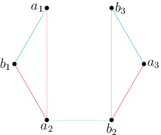
By Lemma 14 and Corollary 13, we may assume that each vertex of the graph $G$ is incident to at least one red edge. Recall that $G$ has 4 or 6 vertices and its blue edges induce a perfect matching. Thus one can easily verify that $G$ either contains an alternative cycle or is isomorphic to the graph drawn on Figure 1. Without loss of generality assume that the latter case holds.

Additionally, we put $V(G)=\{a_{1},a_{2},a_{3},b_{1},b_{2},b_{3}\}$,

see Figures 1 and 2(b). Without loss of generality, we assume that, for all $i$, the directed angle $\measuredangle(a_{i},b_{i})$ does not exceed $\pi$.

Denote by $m_{1}$ and $n_{1}$ the rays emanating from the origin $o$ and passing through the points $a_{1}$ and $b_{1}$, respectively; see Figure 2(a). Denote the rays obtained by the counterclockwise rotation of $m_{1}$ by angles $2\pi/3$ and $4\pi/3$ by $m_{2}$ and $m_{3}$, respectively. Analogously, define $n_{2}$ and $n_{3}$; see Figure 2(a). Applying Corollary 13 to the blue edge $a_{1}b_{1}$, we have $\angle(b_{1},a_{1})<2\pi/3$. Hence the rays

are ordered counterclockwise and divide the plane into 6 regions such that

and

with $\varphi+\psi=2\pi/3$ and $\psi>0$; see Figure 2(a).

Using Corollary 13 for the vertex $a_{2}$, we have that

for any vertex $y\in V(G)\setminus\{a_{1},a_{2}\}$. Therefore, if $\angle(a_{1},a_{2})<2\pi/3$, we can apply Lemma 14 and find an alternating cycle. Hence $\angle(a_{1},a_{2})\geq 2\pi/3$. By Corollary 13, we get

where $\cone A$ stands for the conic hull of a set $A\subseteq\mathbb{R}^{2}$. Analogously, we conclude that

According to our notation, for each $i\in\{1,2,3\}$ there is the counterclockwise rotation by a non-negative angle that maps the ray $oa_{i}$ to the ray $ob_{i}$. Hence the rays

are ordered counterclockwise.

By Corollary 13, we have $\angle(a_{2},b_{3})<2\pi/3$. Since

we conclude that $\measuredangle(a_{2},b_{3})<2\pi/3$, and thus, $b_{2},a_{3}\in\cone\{a_{1},b_{3}\}$; see Figure 2.

The edges $a_{2}b_{2}$ and $a_{3}b_{3}$ belong to $\cone\{m_{2},n_{2}\}$ and $\cone\{m_{3},n_{3}\}$, respectively. Since these cones share only the origin, the line segments $a_{2}b_{2}$ and $a_{3}b_{3}$ do not intersect. Also, they induce a max-sum matching of the point set $\{a_{2},a_{3},b_{2},b_{3}\}$. By the triangle inequality, any max-sum matching of four points in a convex position consists of two intersecting line segments. Hence either $b_{2}$ or $a_{3}$ lies in the convex hull of the remaining endpoints. Without loss of generality assume that

Since the vectors $a_{2}$ and $b_{2}$ are distinct, they are also not collinear.

Denote by $p$ the intersection point of the ray $ob_{2}$ and the line segments $a_{2}b_{3}$. Analogously, denote by $q$ the intersection point of the ray $ob_{2}$ and $a_{2}a_{3}$; see Figure 3. So the point $b_{2}$ lies on the line segment $pq$. Since the ray $ob_{2}$ does not belong to $\cone\{m_{3},n_{3}\}$ containing $a_{3}$ and $b_{3}$, the points $p$ and $q$ are interior for the line segments $a_{2}b_{3}$ and $a_{2}a_{3}$, respectively.

Finally, we finish the proof using the function $f:\{(x,y)\in\mathbb{R}^{2}\times\mathbb{R}^{2}:x\neq y\}\xrightarrow{}\mathbb{R}$ defined by

Comparing the definition of $f$ with (3), we get

Recall that for non-collinear vectors $x,y\neq o$ the ray $o\ell_{xy}$ bisects $\cone\{x,y\}$, that is, $\angle(x,\ell_{xy})=\angle(\ell_{xy},y)$. Also, the point $\ell_{xy}$ lies on the line segment $xy$.

Since $p$ and $q$ are interior points of the line segments $a_{2}b_{3}$ and $a_{2}a_{3}$, respectively, Corollary 16 yields that

Next, we show that these inequalities contradict the equality $f(a_{2},b_{2})=\lambda$.

Since the points $p$ and $q$ lie on the ray $ob_{2}$, we conclude that the points $\ell_{a_{2}p}$ and $\ell_{a_{2}q}$ lie on the ray $o\ell_{a_{2}b_{2}}$. Moreover, the point $\ell_{a_{2}b_{2}}$ belongs to the line segment $\ell_{a_{2}p}\ell_{a_{2}q}$, and thus,

By Lemma 15, we have

a contradiction. Therefore, the graph $G$ contains an alternating cycle, which finishes the proof of Theorem 4. $\square$

Denote by $r_{1}$ and $r_{2}$ the rays emanating from the origin such that $\measuredangle(ox,r_{1})=\measuredangle(r_{2},ox)=2\pi/3$. Thus, we have $\measuredangle(r_{1},r_{2})=2\pi/3$ as well. Since $\angle(x,y)<2\pi/3$ for any $y\in V(G)\setminus\{x\}$, we conclude that no vertex of $G$ lies in $\cone\{r_{1},r_{2}\}$.

Let us show that $\ell_{ab}\not\in\cone\{r_{1},r_{2}\}$ for any blue edge $ab\in\mathcal{M}_{2}$. By Corollary 13, we have $\angle(a,b)<2\pi/3$. Thus, $\cone\{r_{1},r_{2}\}$ and $\cone\{a,b\}$ share only the origin $o$ as $\angle(r_{1},r_{2})=2\pi/3>\angle(a,b)$. By the definition, the point $\ell_{ab}$ lies on a line segment $ab$, and so, $\ell_{ab}\in\cone\{a,b\}$. Therefore, the point $\ell_{ab}$ does not lie in the $\cone\{r_{1},r_{2}\}$, and thus, $\angle(x,\ell_{ab})<2\pi/3$.

By (2), any closed half-plane bounded by a line through the origin must contain $\ell_{ab}$ for some $ab\in\mathcal{M}_{2}$. Among the closed half-planes bounded by the line containing the ray $r_{2}$, choose the one without $x$. This half-plane must contains $\ell_{ab}$ for some $ab\in\mathcal{M}_{2}$. Since no point $\ell_{ab}$ lies in $\cone\{r_{1},r_{2}\}$, we conclude that there is a blue edge $a_{1}b_{1}$ such that

see Figure 4. Analogously, we can find an edge $a_{2}b_{2}\in\mathcal{M}_{2}$ satisfying the inequality

Moreover, by (2) and the above argument on closed half-planes, we can choose $a_{1}b_{1}$ and $a_{2}b_{2}$ in such a way that

For that, it is enough to choose the edges $a_{1}b_{1}$ and $a_{2}b_{2}$ satisfying (4) and (5), respectively, with the maximum possible values of $\measuredangle(x,\ell_{a_{2}b_{2}})$ and $\measuredangle(\ell_{a_{1}b_{1}},x)$. (Here, we use that no point $\ell_{ab}$ lies in $\cone\{r_{1},r_{2}\}$.)

Without loss of generality assume that for $i\in\{1,2\}$, we have

where $0\leq 2\alpha_{i}<\pi$. Moreover, Corollary 13 yields that $\alpha_{i}<\pi/3$. Hence for $i\in\{1,2\}$, we obtain

Since $b_{1}\not\in\cone\{r_{1},r_{2}\}$, we have that $b_{1}\in\cone\{\ell_{a_{1}b_{1}},r_{1}\}$. Analogously, we conclude that $a_{2}\in\cone\{r_{2},\ell_{a_{2}b_{2}}\}$. Therefore,

and so, by Corollary 13, the edge $b_{1}a_{2}$ is red.

To finish the proof, we show that $a_{1}b_{2}$ is also red edge.

First, we claim that $a_{1}\in\cone\{\ell_{a_{1}b_{1}},x\}$ and it does not lie on the ray $ox$. Indeed, it follows from

Analogously, we get that $b_{2}\in\cone\{x,\ell_{a_{2},b_{2}}\}$ and it does not lie on the ray $ox$. Thus the vertex $x$ is distinct from $b_{1}$ and $a_{2}$.

Second, by (6), we have

References

- [1] (2023) Piercing diametral disks induced by edges of maximum spanning trees. In Walcom: Algorithms and computation, C. Lin, B. M. T. Lin, and G. Liotta (Eds.), Cham, pp. 71–77. Note: DOI: https://doi.org/10.1007/978-3-031-27051-2_7. Available at https://arxiv.org/abs/2209.11260 Cited by: §1.
- [2] (2023) On maximum-sum matchings of points. Journal of Global Optimization 85, pp. 111–128. Note: DOI: https://doi.org/10.1007/s10898-022-01199-z. Available at https://arxiv.org/abs/1911.10610 Cited by: §1, §1, §1.
- [3] (2012) Drawing Hamiltonian Cycles with no Large Angles. The Electronic Journal of Combinatorics 19 (2), pp. P31. Cited by: §1.
- [4] (1995) Geometry Junkyard. Centers of maximum matchings. Note: Available at https://www.ics.uci.edu/~eppstein/junkyard/maxmatch.html Cited by: §1, §1, §1.
- [5] (2000) On minimum stars and maximum matchings. Discrete & Computational Geometry 23 (3), pp. 389–407. Cited by: §1, Lemma 3.
- [6] (1993) Convex Analysis and Minimization Algorithms I. Springer Berlin Heidelberg. External Links: Link Cited by: §2.2, Theorem 7, Theorem 8, Theorem 9.
- [7] (2019) Matching points with disks with a common intersection. Discrete Mathematics 342 (7), pp. 1885–1893. Note: Available at https://arxiv.org/abs/1902.08427 Cited by: §1, §1.
- [8] (2022) Intersecting diametral balls induced by a geometric graph. Discrete & Computational Geometry. Note: DOI: https://doi.org/10.1007/s00454-022-00457-x. Available at https://arxiv.org/abs/2108.09795 Cited by: §1, §1, §2.1, Remark 12.
- [9] (2001) Partitions of points into simplices with -dimensional intersection. Part I: the conic Tverberg’s theorem. European Journal of Combinatorics 22 (5), pp. 733–743. External Links: Link Cited by: §1, §1.
- [10] (2021) Tverberg’s theorem, disks, and Hamiltonian cycles. Annals of Combinatorics 25 (4), pp. 995–1005. Note: Available at https://arxiv.org/abs/2011.12218 Cited by: §1.
- [11] (1998) Problem 5. Problem session of the 14th ACM Symposium on Computational Geometry. Note: Available at https://users.cs.duke.edu/~pankaj/scg98-openprobs/open-probs.html Cited by: §1, Conjecture 2.
- [12] (1966) A generalization of Radon’s theorem. Journal of the London Mathematical Society s1-41 (1), pp. 123–128. External Links: Link Cited by: §1.
- [13] (1993) On Generalizations of Radon's Theorem and the Ham Sandwich Theorem. European Journal of Combinatorics 14 (3), pp. 259–264. External Links: Link Cited by: §1, §1.