On the Equivalence of the Weighted Tsetlin Machine and the Perceptron
Abstract
Tsetlin Machine (TM) has been gaining popularity as an inherently interpretable machine leaning method that is able to achieve promising performance with low computational complexity on a variety of applications. The interpretability and the low computational complexity of the TM are inherited from the Boolean expressions for representing various sub-patterns. Although possessing favorable properties, TM has not been the go-to method for AI applications, mainly due to its conceptual and theoretical differences compared with perceptrons and neural networks, which are more widely known and well understood. In this paper, we provide detailed insights for the operational concept of the TM, and try to bridge the gap in the theoretical understanding between the perceptron and the TM. More specifically, we study the operational concept of the TM following the analytical structure of perceptrons, showing the resemblance between the perceptrons and the TM. Through the analysis, we indicated that the TM’s weight update can be considered as a special case of the gradient weight update. We also perform an empirical analysis of TM by showing the flexibility in determining the clause length, visualization of decision boundaries and obtaining interpretable boolean expressions from TM. In addition, we also discuss the advantages of TM in terms of its structure and its ability to solve more complex problems.
1 Introduction
Researchers across various fields are increasingly paying attention to the interpretability of AI techniques. While interpretability previously was inherent in most machine learning approaches, the state-of-the-art methods now increasingly rely on black-box deep neural networks (DNNs). Natively, DNNs can hardly be interpreted during the learning stage or while producing outputs Ghorbani et al. 2019. A surge of techniques attempts to open the black box by visual explanations and gradient-based interpretability Simonyan et al. 2014; Zhang et al. 2018; Radhakrishnan et al. 2018; Bau et al. 2017; Selvaraju et al. 2017, but do not change the black-box nature.
The Tsetlin Machine (TM) is a natively interpretable rule-based machine learning algorithm that produces logical rules Granmo 2018. Despite being logic-based, the TM is a universal function approximator, like a neural network. In brief, it employs an ensemble of Tsetlin Automata (TA) that learns propositional logic expressions from Boolean input features. Propositional logic drives learning, eliminating the requirement for floating-point operations. Due to its Boolean representations and finite-state automata learning mechanisms, it has a minimalistic memory footprint. More importantly, TM achieves interpretability by leveraging sparse disjunctive normal form. Indeed, humans are particularly good at understanding flat and short logical AND-rules, reflecting human reasoning Noveck et al. 1991.
Because the operational concept of TMs is significantly different from that of neural networks, TM is really challenging for those who are used to the neural networks to understand. For this reason, the TMs have not been considered as the to-go method in the machine learning society. In this paper, we show the operational concept of TMs for its learning phase, following the structure that is widely used in the analysis of the neural networks. Particularly, we aim at showing the resemblance between the two distinct techniques and reveal the concept and the advantages of the TMs in a painless manner. In more details, we divide TM’s learning into two phases: the clause learning phase and the clause weight update phase.
For the clause learning phase, we show that one clause can learn one or multiple sub-patterns given enough updates. This phase bears resemblance to the connections and the activation functions in a perceptron. For the clause weight update phase, we indicate that the clauses are weighted according to their correctness, which is similar to the weights in a perceptron. For this reason, following the concept of the perceptron convergence theorem, the clause weight update for the TM can also be confirmed. To summarize, the clauses can learn any sub-patterns from data and the clause weights show the importance of such sub-patterns, similar to the connections and the weights in a perceptron. In addition, we visualize the decision boundaries using clauses of TM and formalize its advantages over other the perceptron.
2 Review of the Tsetlin Machine
The Tsetlin Machine is a machine learning algorithm based on Boolean expressions called clauses that individually identify sub-patterns in data and are aggregated together as a weighted sum of Boolean inputs.
Structure.
A TM in its simplest form takes a feature vector of propositional values as input and assigns the vector a class . In brief, the input vector provides the literal set , consisting of the input features and their negations. By selecting subsets of the literals, the TM can build arbitrarily complex patterns, ANDing the selected literals to form conjunctive clauses:
| (1) |
Above, is the index of a clause and refers to a particular literal . is the total number of clauses. As an example, the clause consists of the literals and evaluates to when and .
The TM assigns one Tsetlin Automata (TA) Tsetlin 1961; Narendra 1989 per literal per clause to build the clauses. The TA assigned to literal of clause decides whether is Excluded or Included in . Figure 1 depicts a two-action TA with states. For states to , the TA performs action Exclude (Action 1), while for states to it performs action Include (Action 2). As feedback to the action performed, the environment responds with either a Reward or a Penalty. If the TA receives a Reward, it moves deeper into the side of the action. If it receives a Penalty, it moves towards the middle and eventually switches action.
With clauses and literals, we have in total TAs. We organize the states of these in an matrix . We will use the function to map the automaton state to Action (Exclude) for states to and to Action (Include) for states to :
| (2) |
We then can connect the states of the TAs assigned to clause with its composition as follows:
| (3) |
Here, is one of the literals and is the state of its TA in clause . The logical imply operator implements the Exclude/Include action. That is, the imply operator is always if (Exclude), while if (Include) the truth value is decided by the truth value of the literal.
Classification.
Classification is performed as a majority vote. The odd-numbered half of the clauses vote for class and the even-numbered half vote for :
| (4) |
As such, the odd-numbered clauses have positive polarity, while the even-numbered ones have negative polarity. As an example, consider the input vector in the lower part of Figure 2. The figure depicts two clauses of positive polarity, and (the negative polarity clauses are not shown). Both of the clauses evaluate to zero, leading to class prediction .
| Input | Clause | 1 | 0 |
| Literal | 1 0 | 1 0 | |
| Include Literal | P(Reward) | NA | 0 0 |
| P(Inaction) | NA | ||
| P(Penalty) | 0 NA | ||
| Exclude Literal | P(Reward) | 0 | |
| P(Inaction) | |||
| P(Penalty) | 0 | 0 0 |
| Input | Clause | 1 | 0 |
|---|---|---|---|
| Literal | 1 0 | 1 0 | |
| Include Literal | P(Reward) | 0 NA | 0 0 |
| P(Inaction) | 1.0 NA | 1.0 1.0 | |
| P(Penalty) | 0 NA | 0 0 | |
| Exclude Literal | P(Reward) | 0 0 | 0 0 |
| P(Inaction) | 1.0 0 | 1.0 1.0 | |
| P(Penalty) | 0 1.0 | 0 0 |
Learning.
The upper part of Figure 2 illustrates learning. A TM learns online, processing one training example at a time. Based on , the TM rewards or penalizes its TAs, which amounts to increasing or decreasing their states. There are two kinds of feedback: Type I Feedback produces frequent patterns and Type II Feedback increases the discrimination power of the patterns.
Type I feedback is given stochastically to clauses with positive polarity when and to clauses with negative polarity when . Conversely, Type II Feedback is given stochastically to clauses with positive polarity when and to clauses with negative polarity when . The probability of a clause being updated is based on the vote sum : . The voting error is calculated as:
| (5) |
Here, is a user-configurable voting margin yielding an ensemble effect. The probability of updating each clause is . Random sampling from will decided which clauses to update, and then the following TA state updates can be formulated as matrix additions, subdividing Type I Feedback into feedback Type Ia and Type Ib:
| (6) |
Here, contains the states of the TAs at time step and contains the updated state for time step (before clipping). The matrices and contain Type I Feedback. A zero-element means no feedback and a one-element means feedback. As shown in Table 2 on the left, two rules govern Type I feedback:
- •
Type Ia Feedback is given with probability whenever both clause and literal are -valued11 1 Note that the probability is replaced by when boosting true positives.. It penalizes Exclude actions and rewards Include actions. The purpose is to remember and refine the patterns manifested in the current input . This is achieved by moving the state of the TA toward the right side. The user-configurable parameter controls pattern frequency, i.e., a higher produces less frequent patterns.
- •
Type Ib Feedback is given with probability whenever either clause or literal is -valued. This feedback rewards Exclude actions and penalizes Include actions to coarsen patterns, combating overfitting. Thus, the selected TA states are decreased.
The matrix contains Type II Feedback to the TAs, given per Table 2 on the right.
- •
Type II Feedback penalizes Exclude actions to make the clauses more discriminative, combating false positives. That is, if the literal is -valued and the clause is -valued, TA that has the current state below are encouraged to move towards right side. Eventually the clause becomes -valued for that particular input, upon inclusion of the -valued literal.
The final updating step for training example is to clip the state values to make sure that they stay within value and :
| (7) |
For example, both of the clauses in Figure 2 receives Type I Feedback over several training examples, making them resemble the input associated with .
2.1 Weighted Tsetlin Machine
In this subsection, we detail the TM with weights. The learning of weights is based on increasing the weight of clauses that receive Type Ia feedback (due to true positive output) and decreasing the weight of clauses that receive Type II feedback (due to false positive output). The overall rationale is to determine which clauses are inaccurate and thus must team up to obtain high accuracy as a team (low weight clauses), and which clauses are sufficiently accurate to operate more independently (high weight clauses). The weight updating procedure is summarized in Algorithm 1. Here, is the weight of clause at the training round (ignoring polarity to simplify notation). The first step of a training round is to calculate the clause output as per Equation (3). The weight of a clause is only updated if the clause output is 1 and the clause has been selected for feedback ( = 1). Then the polarity of the clause and the class label decide the type of feedback given. That is, like a regular TM, positive polarity clauses receive Type Ia feedback if the clause output is a true positive, and similarly, they receive Type II feedback if the clause output is a false positive. For clauses with negative polarity, the feedback types switch roles. When clauses receive Type Ia or Type II feedback, their weights are updated accordingly. We use the stochastic searching on the line (SSL) automaton to learn appropriate weights. SSL is an optimization scheme for unknown stochastic environments Oommen 1997. The goal is to find an unknown location within a search interval . In order to find , the only available information for the Learning Mechanism (LM) is the possibly faulty feedback from its attached environment .
In SSL, the search space is discretized into points, with N being the discretization resolution. During the search, the LM has a location , and can freely move to the left or to the right from its current location. The environment provides two types of feedback: is the environment suggestion to increase the value of by one step, and is the environment suggestion to decrease the value of by one step. The next location of , i.e. , can thus be expressed as follows:
| (8) |
| (9) |
Asymptotically, the learning mechanics is able to find a value arbitrarily close to when and . In our case, the search space of clause weights is , so we use resolution , with no upper bound for . Accordingly, we operate with integer weights. As in Algorithm 1, if the clause output is a true positive, we simply increase the weight by . Conversely, if the clause output is a false positive, we decrease the weight by .
By following the above procedure, the goal is to make low precision clauses team up
by giving them low weights, so that they together can reach the summation target . By teaming up, precision increases due to the resulting ensemble effect. Clauses with high precision, however, obtain a higher weight, allowing them to operate more independently.
The above weighting scheme has several advantages. First of all, increment and decrement operations on integers are computationally less costly than multiplication based updates of real-valued weights. Additionally, a clause with an integer weight can be seen as multiple copies of the same clause, making it more interpretable than real-valued weighting, as shown in the next section. Additionally, clauses can be turned completely off by setting their weights to if they do not contribute positively to the classification task. For a more detailed explanation of the weighted TM, please refer to Abeyrathna et al. 2021.
3 Convergence Analysis of the Tsetlin Machine

As discussed in Section 2, TM learns clauses to identify sub-patterns in data. These sub-patterns are aggregated using a linearly weighted sum of clauses, where the weights depend on how well the clauses detect sub-patterns. Now, let’s consider the weighted TM with clause weights and clauses , where even represent negative polarity clauses and odd represent positive polarity clauses:
| (Using Eq. (5)) |
| (Using Eq. (1)) |
The learning of clauses and its weights can be considered as separate phases as described in Section 2 and shown in Algorithm 1. Each is updated according to its associated clause ’s correctness. Whereas each clause obtains feedback by comparing the clause output (and its polarity) and the true label. So, the convergence of TM is divided into two phases:
- •
Phase : Clause learning - Local sub-pattern learning. A single clause is able to learn a single correct sub-pattern based on the feedback given to it by comparing the clause output with the desired output. This is shown according to parallel feedback given to the TAs. (Local view, see Subsection 3.1)
- •
Phase : Clause weight update - Global pattern aggregation. The sub-patterns learnt by the clauses are weighted according to their correctness, i.e. a weighted sum of sub-patterns. The weighted TM and its weight update is shown to be akin to the perceptron. (Global view, see Subsection 3.2)
3.1 Clause learning
In this subsection, we illustrate that one clause can capture one individual sub-pattern or several sub-patterns if the sub-patterns can be represented by the clause jointly.
To clarify the meaning of capturing one individual sub-pattern or several sub-patterns jointly, we look at the XOR and the AND operators as examples. Let us review the case where one clause captures an individual sub-pattern by looking at the XOR operator. For this operator, (, ) and (, ) give while otherwise. Clearly, we have two sub-patterns and the input bits of the sub-patterns are mutual exclusive. For this reason, we need one clause to capture the first sub-pattern and to represent the second one. Obviously, there is no possibility to represent the two sub-patterns jointly by one clause, and thus one clause must correspond to each sub-pattern. Indeed, the TM can learn almost surely the intended logic in infinite time horizon. The convergence of the XOR operator has been proven in Jiao et al. 2022.
For the case where sub-patterns can be presented jointly, we exam the AND operator. Clearly, in addition to (, ) and (, ), (, ) will also trigger a positive output. Different from the XOR case where the sub-patterns are mutually exclusive, the latter two sub-patterns in the AND operator can be jointly represented by . Although in the AND operator three sub-patterns exist, two clauses, e.g., and , are sufficient to present the intended AND operator. Indeed, the TM can learn almost surely the intended AND operator in infinite time horizon. The convergence of the operator has been proven in Jiao et al. 2021.
From the above mentioned two examples, we can see that a clause can indeed learn either a sub-pattern individually or multiple sub-patterns jointly for those special cases where the input is 2-bits long. In general, we conjuncture that a clause, after learning, can capture one or multiple sub-patterns from the training sample when the input has more bits. The proof of the general case is not trivial because the feedback for a certain literal is not only determined by its own state, but also by the output of the clause that is jointly determined by all its literals. Although this conjuncture has not been theoretically proven, we have observed from simulations that the clauses in a TM can indeed present sub-patterns efficiently. In what follows, we present the clause learning phase formally, aiming at revealing the dynamics of the learning and providing more insights for a better comprehension.
TM learns to recognize local patterns courtesy of clauses, which are propositional expressions of binarized features (literals), in original or negated form, connected by logical AND operations. Correct sub-patterns are learnt by updating TA states that are associated with each literal which thereafter results in updated clauses. Consider a sub-pattern or a group of sub-patterns that one clause can learn joint. For the weighted TM, output is expected to be greater than once learnt for the intended sub-pattern (or joint sub-patterns), i.e.,
| (10) |
Each TA , associated with a particular literal , is updated according to the feedback given to the clause. The update of is to be discussed in the next Subsection. For updating the clause itself, we have
| (11) |
where is the feedback given to the clause by comparing , the clause output and , the true label. This feedback is sent to each literal. Note that once the feedback is given, the state updating process for each TA is independent and thus the TAs can be updated in parallel.
As the literals within the clause have an AND relationship, any literal that produces 0 will results in a 0 for the clause output. On the contrary, the clause output 1 only when all literals output 1. This nature will result in a 0 value for a clause most probably when we randomly initiate the states of the TAs in the beginning of the learning. The 0 literal value or clause value will result in a Type Ib feedback for any “true” training samples (), which encourages the literals to be excluded. As the literals become excluded, the length of the clause is reduced. Once the 0-valued literals are all excluded and only the 1-valued literals are left, Type Ia feedback will come to the play and thus encourage more literals to be included in the clause. At the same time, Type II feedback will depress possible false positive by including necessary literals upon a false training sample (). This process will go back and forth during the learning process, until reaches . Once holds, the input of the sub-pattern is blocked by the TM, as per Eq. (5).
3.2 Clause weight update
As the clause is update to learn the intended sub-pattern, each clause is weighted according its importance and correctness. Here, the importance of the sub-pattern depends on its frequency of occurrence in different instances of data and its distinguishing capabilities for a particular task. For example, a clause that captures the sub-pattern of facial features in a “dog vs cat” task will have higher weights than a clause that captures sub-patterns of the tail, since facial feature are more discriminative for this task. The weighted TM can be represented as follows:
which can be rewritten as:
| (12) |
where is the clause weight of clause and is the threshold. Clauses are represented in Equation (3). This means that if this inequality holds for a particular input then it is assigned to class , otherwise class . For the case of TM, the threshold is static and assigned at the beginning of training. Here, we make learnable by reconstructing it as a clause weight. The clause associated with is a dummy clause whose output is always . And, the weight is always subtracted from the weighted clause vote count. After those modifications, Eequation (12) becomes analogous to a perceptron Rosenblatt 1958, where are the weights, are the inputs and is the bias. Now, the weights of such a network are updated by the gradients of the error with respect to the weights. Let the error be represented as:
| (13) |
where, is the correct target. Clearly, the gradient of with respect to weight becomes:
| (14) |
which means that the weight is updated as:
| (15) | ||||
where represents correct prediction with and incorrect prediction with . This gives the direction of update and is the learning rate. In case of perceptron, , which makes perceptron update:
| ([since ]) | |||
| (16) |
This is how the clause weights are updated in weighted TM as shown in Section 2 and Algorithm 1. From Algorithm 1, we can see that, when the clause is correct, Equation (16) is used to update the clause weight as shown in Lines and in case of the clause being incorrect, Equation (16) is used to update the clause weight as shown in Lines . The clause weights with clause output are not updated.
Algorithm 1 runs over all training instances (in batches or online manner) and the clause weights are incremented every time the clause detects the correct sub-pattern and decremented if it does not. As mentioned previously, the weights of clauses that capture important and more discriminative sub-patterns, i.e. ones that reduce the error and produce correct outputs, are incremented gradually and vice versa.
Similarly, gradient of error in Equation (13) with respect to is:
| (17) |
Applying Equation (15) to update , we have:
| (18) |
From Equation (18), we can see that is updated with the opposite polarity as , which is what we expected as is always subtracted from the total vote count. This shows that the weight updating mechanism in the TM can be considered a special case of a perceptron with binary inputs (assuming the outputs of clauses are inputs here). Hence, the convergence properties and mathematical analysis of the perceptron Rosenblatt 1958 also hold for the clause weight update of the TM, assuming the clauses as binary inputs. In addition, the clause weight update is equivalent to a gradient update with . The convergence of perceptron is given as a reference point in Appendix A.
4 Empirical Analysis
In this section, we present the empirical results based on our experiments. We firstly show the results for the clause learning phase with the focus on the relationship between the clause length and hyperparameter . Thereafter, we consider the weights of the TM and show the resemblance between the neural networks and the TM.
4.1 Clause Length
A clause evaluating to means that the sub-pattern associated with the clause is presented in a particular data instance and a clause evaluating to means the absence of the sub-pattern (but might to evaluate to for other instances, indicating presence of the sub-pattern). Understandably, if the length of a clause is longer, it learns more fine features or details in the sub-pattern. This is due to more literals are included for a longer clause so that the details/fine features can also be represented, with a cost of the risk of overfitting. On the contrary, the short clause learns more generalized features and has easier readability. The length of the clause is depend on the nature of the problem, and also in part, depends on the -parameter. The -parameter is responsible for assigning the probabilities of reward, penalty and inaction for including and excluding literals (as given in Table 1). From Table 1, we can see that the probability on inclusion of a literal is high when is high, mainly due to Type Ia feedback. To validate this statement, we show from Table 3 the variation in clause size as a function of -parameter. These clauses were obtained by training a TM on the Iris dataset for epochs. Clearly, longer clauses are found for a lager value of .
| Clause-1: | ||
|---|---|---|
| Clause-2: | ||
| Clause-3: | ||
| Clause-4: | ||
| Clause-5: | ||
| Clause-6: | ||
| Clause-7: | ||
| Clause-8: | ||
| Clause-9: | ||
| Clause-10: | ||
| Clause-11: | ||
| Clause-12: |
A comparison between two different values of the -parameter on memory consumption, training time and number of epochs required to reach accuracy on the Iris dataset is presented in Table 4. For this task, a TM consisting of clauses is employed. Clearly, the TM with smaller value requires less memory due to the less included literals. For the same reason, a shorter training time per epoch is also achieved. Nevertheless, the smaller requires more training epochs to obtain the same accuracy, which requires slightly more overall training time. Even though these are different configurations of TM, both are capable of achieving comparable performance. The -parameter is an important hyperparameter which needs to be carefully tuned to obtain optimal performance and interpretability. A detailed analysis and comparison of TM’s memory and time consumption with other algorithms has been shown in Lei et al. 2020 and a more rigorous theoretical analysis of the parameter can be found in Zhang et al. 2022.
| Memory (in Kb) | 204.8 | 122.5 |
|---|---|---|
| Epochs | 250 | 350 |
| Training time per epoch (in millisec) | 7.26 | 5.53 |
4.2 Visualization of Decision Boundaries
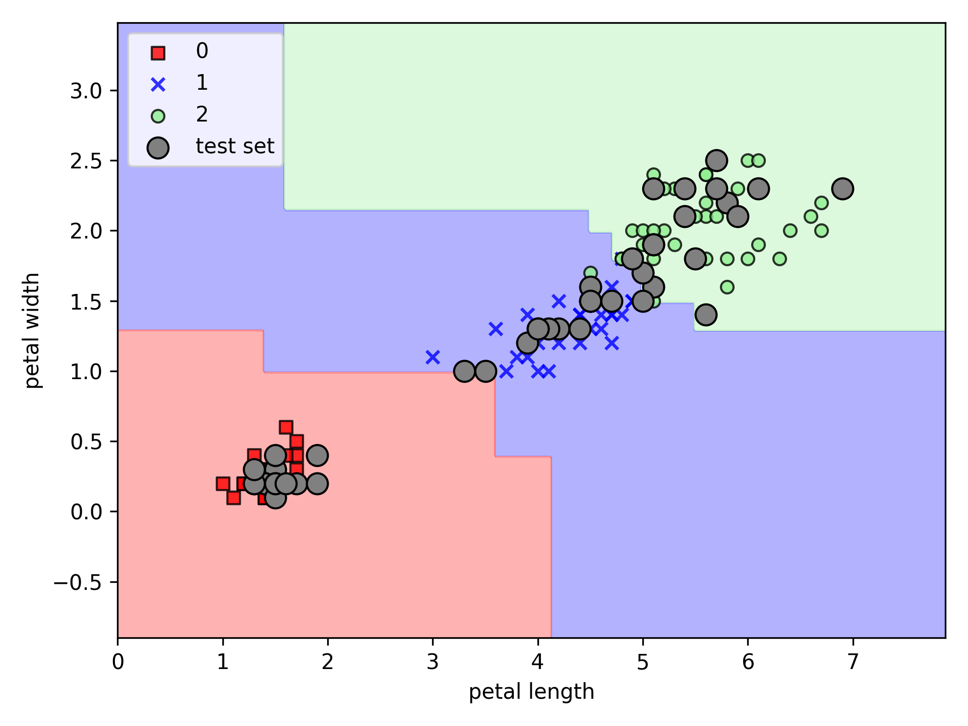
Visualizing decision boundaries is the one of the simplest ways of determining the pattern recognition abilities of an algorithm. It offers perspective about the decision function learnt by the method in order to best distinguish between patterns belonging to different categories. In this subsection, we visualize the decision boundaries of TM, perceptron and a single layer neural network (SLNN) with ReLU activation.
Figure 4 shows the visualization of decision boundaries for TM, perceptron and SLNN obtained from testing on the Iris dataset. Each model was trained on the Iris dataset for epochs. The TM consisted of clauses and the SLNN was made up of neurons in the hidden layer activated by the ReLU function. The TM, perceptron and SLNN obtained , and accuracy on the testing set, respectively22
2
The code to reproduce these results and visualize decision boundaries is available here: github.
As we can see from Figure 4(a), the decision boundaries of TM are cumulatively formed from clauses. Each clause contributes to the decision boundary as . Basically, the decision boundary formed is in the form of steps by filled contour lines. TM’s decision boundary is like an unsmooth approximated version of a non-linear neural network, shown in Figure 4(c). However, in case of a new data point, the entire curved decision boundary of a neural network might have to be changed in order to accommodate for the new data point. Whereas for TM, a clause (or a set of clauses) can simply learn the new pattern and create a step in the decision boundary to include the new data point in the correct region. Note that decision boundaries can vary depending upon initialization and learning trajectory of TM.


To show that TM has the capability to separate non-linearly separable patterns, we show a toy like example, namely the TM’s decision boundaries for the XOR problem in Figure 5. The perceptron or linear neural networks are incapable of solving the XOR problem. However, as can be seen from Figure 5, TM can create decision boundaries that separate such patterns courtesy of the clauses. Each clauses contributes in the construction of the decision boundary. Here, we use clauses to learn the XOR sub-patterns. The theoretical analysis of convergence of TM on the XOR problem can be found in Jiao et al. 2022.

4.3 Interpretability
As previously explained, each propositional expression is a conjunctive clause, consisting of feature,
in their original or negated forms, interacting with each other using logical AND operations.
These clauses can form a simplified representation of the arm selection policy by combining them into
a single Disjunctive Normal Form (DNF) expression. Since clauses are assigned to each class of the
multiclass problem, we can produce a single DNF expression for each class. These DNF expressions are
propositional logic expressions made up of binarized features. The TM is able to produce these
interpretations demonstrating how it interprets the context with respect to each arm.
Here, we show the simplified propositional expressions for each class, obtained from TM trained on the Iris dataset:
- 1.
- Class-1:
- Class-2:
- Class-3:
- Class-1:
The above expressions are obtained by combining the top ten highest weighted positive clauses for each class by OR-ing them and just simplifying the Boolean expressions33 3 Requires a couple of lines of code using the Sympy library..
5 Discussions
5.1 Tsetlin Machine vs Deep Learning
TM is a machine learning algorithm based on propositional Boolean expressions and logical operations. It is able to compete in performance with much larger deep learning models containing hundreds of thousands to many millions of floating point parameters. Different from deep neural networks, TM consists of a few thousands of binary clauses Sharma et al. 2021; Yadav et al. 2021a, resulting in simplicity and low memory and energy consumption Lei et al. 2020. This feature makes TM suitable for mobile computing and federated learning in power constraint IoT devices. In addition, the propositional-logic based clauses are more interpretable than float-number based operations utilized in deep neural networks.
Similar to deep learning, TM is also prone to overfitting. In other words, TM also learns patterns related to noise in the training data. For example, TM is able to achieve training accuracy on large datasets like CIFAR-100, but the performance drops during validation . To mitigate the overfitting problem, a new version of TM, called the Drop Clause TM Sharma et al. 2021, has been proposed, which reduces redundancy and improves the generalization capabilities of TM.
5.2 Tsetlin Machine vs Perceptron
As shown in Section 3.2, the weight update in TM can be considered as a special case of the perceptron learning algorithm for binarized input. Additionally, TM has a phase of learning in the clause level, i.e. representing a sub-pattern by a clause, which gives it better representability and flexibility. Figs. 6(a) and 6(b) show the difference in structures of the TM and perceptron. The number of learnable parameters in the perceptron is restricted by the number of inputs. On the contrary, in TM, the number of clauses can be configured independently to the input’s dimension, giving it structural flexibility.
Based on the descriptions in Section 2, we understand that the operational concept of the T is modularized, which has three parts. Firstly, distinct clauses learn various local sub-patterns. Secondly, the weights are assigned to these clauses according to their importance in solving the task. Finally, these sub-patterns are combined for the final classification.
On the other hand, the perceptron has to learn global patterns directly from data in a single phase, limited to solving linearly separable patterns, whereas TM has demonstrated its competence in solving much more complex problems Sharma et al. 2021; Yadav et al. 2021b; Yadav et al. 2021c; Yadav et al. 2021a; Granmo et al. 2019; Abeyrathna et al. 2020b; Abeyrathna et al. 2020a; Berge et al. 2019, which traditional machine learning algorithms are incapable of.


6 Conclusions
In this paper, we try to bridge the gap between the perceptron (and single-layer neural network) and TM by showing the similarities that lie in their respective structure and learning procedures. We formalize the learning mechanism of TM by dividing the learning phase into two layers. We show the equivalence of TM’s weight update phase with the perceptron learning algorithm. An empirical analysis and visualization of decision boundaries demonstrates how TM can solve nonlinearly separable patterns, like the XOR problem, which the perceptron (and linearly activated SLNN) is incapable of. The decision boundaries show similarities to that of the single-layer neural network. Apart from visualization of decision boundaries, the empirical analysis also shows the flexibility of determining clause length, memory consumption, convergence rate and obtaining interpretable Boolean rules.
References
- Abeyrathna et al. [2020a] K. Darshana Abeyrathna, Ole-Christoffer Granmo, Xuan Zhang, Lei Jiao, and Morten Goodwin. The Regression Tsetlin Machine - A Novel Approach to Interpretable Non-Linear Regression. Philosophical Transactions of the Royal Society A, 378, 2020.
- Abeyrathna et al. [2020b] K. Darshana Abeyrathna, Harsha S. Gardiyawasam Pussewalage, Sasanka N. Ranasinghea, Vladimir A. Oleshchuk, and Ole-Christoffer Granmo. Intrusion Detection with Interpretable Rules Generated Using the Tsetlin Machine. In 2020 IEEE Symposium Series on Computational Intelligence (SSCI). IEEE, 2020.
- Abeyrathna et al. [2021] Kuruge Darshana Abeyrathna, Ole-Christoffer Granmo, and Morten Goodwin. Extending the Tsetlin Machine With Integer-Weighted Clauses for Increased Interpretability. IEEE Access, 9, 2021.
- Bau et al. [2017] David Bau, Bolei Zhou, Aditya Khosla, Aude Oliva, and Antonio Torralba. Network dissection: Quantifying interpretability of deep visual representations. CoRR, abs/1704.05796, 2017.
- Berge et al. [2019] Geir Thore Berge, Ole-Christoffer Granmo, Tor Oddbjørn Tveit, Morten Goodwin, Lei Jiao, and Bernt Viggo Matheussen. Using the Tsetlin Machine to Learn Human-Interpretable Rules for High-Accuracy Text Categorization with Medical Applications. IEEE Access, 7:115134–115146, 2019.
- Ghorbani et al. [2019] Amirata Ghorbani, Abubakar Abid, and James Zou. Interpretation of neural networks is fragile. Proceedings of the AAAI Conference on Artificial Intelligence, 33(01):3681–3688, Jul. 2019.
- Granmo et al. [2019] Ole-Christoffer Granmo, Sondre Glimsdal, Lei Jiao, Morten Goodwin, Christian W. Omlin, and Geir Thore Berge. The Convolutional Tsetlin Machine. arXiv preprint arXiv:1905.09688, 2019.
- Granmo [2018] Ole-Christoffer Granmo. The Tsetlin Machine - A Game Theoretic Bandit Driven Approach to Optimal Pattern Recognition with Propositional Logic. arXiv preprint arXiv:1804.01508, 2018.
- Jiao et al. [2021] Lei Jiao, Xuan Zhang, and Ole-Christoffer Granmo. On the Convergence of Tsetlin Machines for the AND and the OR Operators. https://arxiv.org/abs/2109.09488, 2021.
- Jiao et al. [2022] Lei Jiao, Xuan Zhang, Ole-Christoffer Granmo, and K Darshana Abeyrathna. On the Convergence of Tsetlin Machines for the XOR Operator. IEEE Trans. Pattern Anal. Mach. Intell., 2022.
- Lei et al. [2020] Jie Lei, Adrian Wheeldon, Rishad Shafik, Alex Yakovlev, and Ole-Christoffer Granmo. From arithmetic to logic based ai: A comparative analysis of neural networks and tsetlin machine. In 2020 27th IEEE International Conference on Electronics, Circuits and Systems (ICECS), pages 1–4, 2020.
- Narendra [1989] Kumpati S. Narendra. Learning automata : an introduction. Prentice Hall, Englewood Cliffs N.J., 1989.
- Noveck et al. [1991] I. Noveck, R. B. Lea, George M. Davidson, and D. O’brien. Human reasoning is both logical and pragmatic. Intellectica, 11:81–109, 1991.
- Oommen [1997] B.J. Oommen. Stochastic searching on the line and its applications to parameter learning in nonlinear optimization. IEEE Transactions on Systems, Man, and Cybernetics, Part B (Cybernetics), 27(4):733–739, 1997.
- Radhakrishnan et al. [2018] Adityanarayanan Radhakrishnan, Charles Durham, Ali Soylemezoglu, and Caroline Uhler. Patchnet: Interpretable neural networks for image classification, 2018.
- Rosenblatt [1958] Frank Rosenblatt. The perceptron: a probabilistic model for information storage and organization in the brain. Psychological review, 65(6):386, 1958.
- Selvaraju et al. [2017] Ramprasaath R. Selvaraju, Michael Cogswell, Abhishek Das, Ramakrishna Vedantam, Devi Parikh, and Dhruv Batra. Grad-cam: Visual explanations from deep networks via gradient-based localization. In 2017 IEEE International Conference on Computer Vision (ICCV), pages 618–626, 2017.
- Sharma et al. [2021] Jivitesh Sharma, Rohan Yadav, Ole-Christoffer Granmo, and Lei Jiao. Drop Clause: Enhancing Performance, Interpretability and Robustness of the Tsetlin Machine. arXiv e-prints, page arXiv:2105.14506, May 2021.
- Simonyan et al. [2014] Karen Simonyan, Andrea Vedaldi, and Andrew Zisserman. Deep inside convolutional networks: Visualising image classification models and saliency maps, 2014.
- Tsetlin [1961] Michael Lvovitch Tsetlin. On behaviour of finite automata in random medium. Avtomat. i Telemekh, 22(10):1345–1354, 1961.
- Yadav et al. [2021a] Rohan K Yadav, Lei Jiao, Ole-Christoffer Granmo, and Morten Goodwin. Human-level interpretable learning for aspect-based sentiment analysis. Proceedings of the AAAI Conference on Artificial Intelligence, 35(16):14203–14212, May 2021.
- Yadav et al. [2021b] Rohan Kumar Yadav, Lei Jiao, Ole-Christoffer Granmo, and Morten Goodwin. Distributed Word Representation in Tsetlin Machine. arXiv preprint arXiv:2104.06901, 2021.
- Yadav et al. [2021c] Rohan Kumar Yadav, Lei Jiao, Ole-Christoffer Granmo, and Morten Goodwin. Interpretability in Word Sense Disambiguation using Tsetlin Machine. In 13th International Conference on Agents and Artificial Intelligence (ICAART 2021). INSTICC, 2021.
- Zhang et al. [2018] Quanshi Zhang, Ying Nian Wu, and Song-Chun Zhu. Interpretable convolutional neural networks. In Proceedings of the IEEE Conference on Computer Vision and Pattern Recognition, pages 8827–8836, 2018.
- Zhang et al. [2022] Xuan Zhang, Lei Jiao, Ole-Christoffer Granmo, and Morten Goodwin. On the Convergence of Tsetlin Machines for the IDENTITY- and NOT Operators. IEEE Trans. Pattern Anal. Mach. Intell., 44(10):6345–6359, 2022.
Appendix
Appendix A Convergence of Perceptron
Let be the weights of the perceptron and be the input-label pairs, where and each is a -dimensional vector. Assumptions:
- 1.
There exists some such that , and for some , :
(19) - 2.
Also assume, :
(20)
Perceptron Convergence:
The number of updates required for the perceptron to converge to a local minimum is bounded by:
| (21) |
Proof:
Let be the weight vector after update and . So, for we have:
It follows by induction on that:
In addition, as , then we have:
| (22) |
Now, we can also write:
It follows by induction on that:
| (23) |
Combining equations 22 and 23, we have:
| (24) | |||
| (25) |
This shows that the number of update steps, , required by the perceptron to obtain a local minimum, is bounded. In case of TM, the same proof above holds with only one difference: , , i.e. the input is a binary vector. As the (Frobenius) norm of a binary vector is the square root of the number of non-zero elements and the number of non-zero elements can be atmost . So, the second assumption becomes:
| (26) |
So, for TM, Equation (25) becomes:
| (27) |